\AtAppendix

Counterbalancing Learning and Strategic Incentives in Allocation Markets

Jamie Kang
Stanford University
kangjh@stanford.edu
&Faidra Monachou
Stanford University
monachou@stanford.edu
Moran Koren
Harvard University
me@mkoren.org
&Itai Ashlagi
Stanford University
iashlagi@stanford.edu
Abstract

Motivated by the high discard rate of donated organs in the United States, we study an allocation problem in the presence of learning and strategic incentives. We consider a setting where a benevolent social planner decides whether and how to allocate a single indivisible object to a queue of strategic agents. The object has a common true quality, good or bad, which is ex-ante unknown to everyone. Each agent holds an informative, yet noisy, private signal about the quality. To make a correct allocation decision the planner attempts to learn the object quality by truthfully eliciting agents’ signals. Under the commonly applied sequential offering mechanism, we show that learning is hampered by the presence of strategic incentives as herding may emerge. This can result in incorrect allocation and welfare loss. To overcome these issues, we propose a novel class of incentive-compatible mechanisms. Our mechanism involves a batch-by-batch, dynamic voting process using a majority rule. We prove that the proposed voting mechanisms improve the probability of correct allocation whenever agents are sufficiently well informed. Particularly, we show that such an improvement can be achieved via a simple greedy algorithm. We quantify the improvement using simulations.

1 Introduction

This paper contributes to the growing literature in the intersection of learning and mechanism design, by considering a fundamental allocation problem in the presence of learning and strategic agents. In our setting, a planner needs to allocate a single indivisible object to at most one among several agents waiting in a queue. The object’s true quality is either high (“good”) or low (“bad”), but is ex-ante unknown to both the planner and the agents. Agents are privately informed, in the sense that each receives a private signal that is informative about the true quality of the object, and strategic since they choose to accept or reject the object based on the action maximizing their expected utility. In this framework, agents thus engage in a social learning process as they observe the actions of their predecessors but not their private signals. The planner’s goal is to design an incentive-compatible mechanism that optimizes correctness, i.e., maximizes the ex-ante accuracy of allocation.

This problem finds a natural application in the allocation of donated organs to patients on a national waitlist. The median waiting time for a first kidney transplant in the U.S. is around 3.6 years [25], whereas the rate at which deceased donor kidneys are offered to patients but eventually discarded has been growing steadily [23], exceeding $21.2\%$ in 2020 [30]. The reasons leading to high discard rates – even of seemingly high-quality organs – remain unclear. Clinical studies attribute this increase to herding behavior and inefficiency in allocation mechanisms [29, 11]. Improving the allocation outcome of these markets is undoubtedly crucial as it could save thousands of future lives.

Towards understanding the source of high discard rates, our framework highlights the often overlooked role of social learning. In most cases, when offered an organ, patients not only have access to publicly available data about the organ (e.g., donor’s age, organ size) but also consult with their own physicians for private opinions. Each physician may assess the same organ differently based on their prior experience and/or medical expertise. Empirical works [13, 31] have recently proposed an explanation that patients rationally ignore their own private information (e.g., a physician’s medical assessment) about the quality of an organ and follow the preceding patients’ rejections.

Our proposed model captures this phenomenon and serves as a theoretical sandbox for the design and assessment of alternative allocation policies. We theoretically show that sequentially offering the object to agents – which is a policy commonly used in practice – can result in poor correctness, since the rejections by the few initial agents can cause a cascade of rejections by the subsequent agents.

To address this issue, we introduce a novel class of incentive-compatible allocation mechanisms characterized by a batch-by-batch, dynamic voting process under a simple majority rule. Our proposed greedy mechanism dynamically partitions the list into batches of varying sizes. Then, it sequentially offers the object to each batch until the object is allocated to some agent. The planner privately asks each agent in the current batch to either opt in or opt out. If the majority of the current batch vote to opt in, then the planner randomly allocates the object to one of the current agents who opted in. If the mechanism exhausts the list without success, the object is discarded. Interestingly, several Organ Procurement Organizations (OPOs) already offer organs in batches, although no voting is used;111Based on authors’ personal communication. See, e.g., [21] for allocation in batches. the reasons are both to speed up the allocation process and to avoid herding.

In our main result, we show that if private signals are at least as informative as the prior, there always exists an incentive-compatible voting mechanism that strictly improves correctness and thus helps avoid unwanted discards. Furthermore, we suggest a simple, greedy algorithm to implement such a mechanism. For all other values of private signal precision, we establish that there is no incentive-compatible voting mechanism. Moreover, every voting mechanism results in the same correctness as the sequential offering mechanism.

Incentive-compatible voting mechanisms have several interesting properties. First, the batch size increases after each failed allocation attempt. The intuition is simple. Failed allocations make the current belief about the object quality more pessimistic. Therefore, the planner increases the batch size to ensure that the object is allocated only if a sufficient number of agents receive positive signals while each agent’s decision remains pivotal. Second, offering to another batch after a failed attempt strictly improves correctness (compared to sequential offering). As our simulations showcase, this improvement is significant and generally becomes larger as the prior and signal precision grow; in fact, a voting mechanism with just two batches significantly outperforms sequential offering. Finally, we find that the prior and signal precision have opposite effects on correctness: the correctness tends to decrease as the prior increases but the marginal effect of signal precision is positive. An intuitive explanation is as follows. Since the optimal batch size decreases as the prior increases, the probability to incorrectly allocate a bad object increases. However, as the signal precision improves, the magnitude of the error decreases since agents’ signals become more reliable.

We highlight the tension between agents’ strategic incentives and the planner’s learning goal. From the planner’s perspective, agents’ private signals contain valuable information about the unknown quality of the object. By increasing the number of collected data points, the planner can improve her confidence about the true quality of the object. Agents’ strategic incentives, however, impose a constraint on the maximum size of the batch that allows the truthful elicitation of agents’ signals: as the batch size increases, the chance to be pivotal decreases which in turn reduces the incentive for an agent with a negative signal to be truthful. Our proposed voting mechanisms enable the planner to crowdsource agents’ private information in a simple, truthful, and effective manner.

Related literature. Our model draws upon seminal social learning papers [7, 8, 28] and their extensions in various game structures [1, 14, 24, 2]. Several empirical studies also examine social learning in organ allocation settings [31, 13]. However, none of these works consider the existence of a planner that controls the flow of information. Furthermore, our proposed mechanism is inspired by the voting literature (e.g., [12, 6]); our notion of correctness is adopted from [3]. Finally, our paper is loosely connected to information design (e.g., [18, 27, 26, 10]) and Bayesian exploration (e.g., [20, 16, 22, 15, 17]). In contrast to our model, this literature does generally not consider an underlying social learning process. We include an extended overview of the related literature in Appendix A.

2 Model

We consider a model in which a social planner wishes to allocate a single indivisible object of unknown quality to privately informed agents in a queue.

Object and agents. The object is characterized by a fixed quality $\omega\in\{G,B\}$, where $G$ and $B$ denote a good and bad quality, respectively. The true quality $\omega$ of the object is ex-ante unknown to both the planner and agents; however, both share a common prior belief ${\mu=\mathbb{P}(\omega=G)\in(0,1).}$

Agents are waiting in a queue; we denote by $i$ the agent in position $i.$ Each each agent knows his own position. For simplicity, we assume that the queue consists of an arbitrarily large number $I$ of agents. Each agent $i$ has a private binary signal $s_{i}\in\mathcal{S}\triangleq\{g,b\}$ that is informative about the true quality of the object $\omega.$ Each $s_{i}$ is identically and independently distributed conditional on $\omega.$ Furthermore, each $s_{i}$ is aligned with $\omega$ with probability ${q=\mathbb{P}(s_{i}=g\mid\omega=G)=\mathbb{P}(s_{i}=b\mid\omega=B),}$ where the signal precision $q\in(0.5,1)$ is commonly known.222The condition $q\in(0.5,1)$ is without loss of generality. The common prior belief $\mu$ and signal precision $q$ are standard in the social learning literature [7, 8, 28].

Agents are risk-neutral. The utility of the agent who receives the object is $1$ if $\omega=G$ and $-1$ if $\omega=B$ (This symmetry simplifies the exposition and analysis but does not qualitatively change the results.). Any agent who does not receive the object, because he either declines or is never offered, receives a utility of 0. As a tie-breaking rule we assume that indifferent agents always decline.

Voting mechanisms. The planner designs a mechanism which potentially asks (a batch of) agents to report their private signals, and based on their report, decides whether and how to allocate the object. We consider a class of voting mechanisms denoted by $\mathcal{V}.$ A voting mechanism $V\in\mathcal{V}$ offers the object sequentially to odd-numbered batches of agents, where each batch size may be set dynamically based on the information from previous batches. In any given batch, if the majority of agents vote to opt in, the object is allocated uniformly at random to one of the current agents who opted in.

Formally, a voting mechanism $V_{\{\pi_{j}\}_{j=1}^{\infty}}$ is defined by a sequence of functions $\pi_{1},\pi_{2},...$, such that for each batch $j,$ the corresponding function $\pi_{j}:[0,1]\rightarrow\mathbb{N}$ maps a current belief $\mu_{j-1}$ about the object quality $\omega$ to a batch size $K_{j}$ (we let $\mu_{0}=\mu$). The mechanism begins with offering to the first batch of agents, who are in positions $1,\ldots,\pi_{1}(\mu)$. If the object is not allocated to batch $j-1,$ it is offered to the agents in the next $\pi_{j}(\mu_{j-1})$ positions.

When batch $j$ is offered the object, each agent $i$ in batch $j$ chooses an action (a vote) $\alpha_{i}\in\mathcal{A}\triangleq\{y,n\}$, where $y$ and $n$ correspond to opting in (“yes”) and opting out (“no”), respectively. If $Y_{j},$ the number of opt in votes from batch $j$, constitutes the majority of batch $j$, i.e., $Y_{j}\geq\lceil\frac{\pi_{j}(\mu_{j-1})}{{2}}\rceil$, the object is allocated uniformly at random among agents in batch $j$ who opt in. To simplify exposition, we sometimes denote by $K_{j}$ the ex-post size of batch $j$ (while omitting the dependency on the current belief $\mu_{j-1}$). We assume that the agents in batch $j$ as well as the planner observe all the votes of agents in the previous batches $j^{\prime}<j$, and this is commonly known. After any batch $j$ and given a current prior $\mu_{j-1}$, the belief $\mu_{j}$ shared by the planner and agents is updated recursively in terms of the realized batch size $K_{j}$ and voting outcome $Y_{j}$ as

$$\mu_{j}\triangleq\mathbb{P}\left(\omega\mid\mu_{j-1},K_{j},Y_{j}\right)=\frac{\mu_{j-1}q^{Y_{j}}(1-q)^{K_{j}-Y_{j}}}{\mu_{j-1}q^{Y_{j}}(1-q)^{K_{j}-Y_{j}}+(1-\mu_{j-1})q^{K_{j}-Y_{j}}(1-q)^{Y_{j}}}.$$ (1)

A commonly applied voting mechanism is a sequential offering mechanism, which offers the object to one agent at a time. Another type of voting mechanism is single-batch voting mechanisms, which offer the object only once; thus, the object is discarded if the majority in the batch choose to opt out.

Let $u_{i}(\alpha_{i};s_{i})$ denote the expected utility of an agent who receives signal $s_{i}\in\mathcal{S}$ and takes action $\alpha_{i}\in\mathcal{A}$. A voting mechanism $V\in\mathcal{V}$ is incentive-compatible (IC) if $u_{i}(y;g)\geq u_{i}(n;g)$ and $u_{i}(n;b)\geq u_{i}(y;b).$ Thus, agent $i$ gets higher utility from opting in than opting out when he has received signal $s_{i}=g$, but prefers to opt out when $s_{i}=b$.

Correctness. The planner’s goal is to maximize the probability of a correct allocation outcome, or correctness; the allocation outcome is correct if it allocates a good object or does not allocate a bad object. Formally, under a voting mechanism $V\in\mathcal{V}$, the planner’s decision whether to allocate the object or not is denoted by the random variable $Z=\{0,1\}.$

A mechanism $V\in\mathcal{V}$ achieves correctness $c(V)$ if

$\displaystyle c(V)\triangleq\mathbb{E}_{V}\left[\mathbb{I}(\omega=G\,\cap\,Z=1)+\mathbb{I}(\omega=B\,\cap\,Z=0)\right].$

Since we allocate a single object, a cascade can only form on the opt out action. Therefore, maximizing correctness is equivalent to maximizing social welfare.

Upper bound on correctness. A natural benchmark on correctness would be the optimal solution in a setting where agents are not strategic and thus are willing to truthfully reveal their private signal to the planner. In the absence of strategic incentives, the planner’s optimal solution would be to (i) ask all agents in the queue to reveal their private signals, (ii) compute her posterior belief based on the gathered information, and (iii) allocate the object to a random agent if and only if her posterior exceeds 0.5. Equivalently, as we show in Lemma 1 in Appendix B, the planner allocates the object if and only if the number of positive signals is at least ${\underline{y}\triangleq 0.5\,\log\left(\frac{1-\mu}{\mu}\right)\left(\log\left(\frac{q}{1-q}\right)\right)^{-1}+0.5\,I},$ where $I$ is the number of agents in the queue. In that case, we can show that correctness equals

$$\mathbb{P}\left(X_{I}\geq\underline{y}\right),$$ (2)

where $X_{I}$ is a Binomial$(I,q)$ random variable (see also Lemma 2). As $I$ grows, correctness approaches 1. Importantly, this upper bound is not achievable by an incentive-compatible mechanism.

Discussion of modeling assumptions. The model is based on several modeling choices that we discuss next. First, the assumption that voting outcomes are fully revealed to subsequent batches is made for simplicity. Dropping this knowledge complicates the analysis substantially: one should compute a posterior belief of an agent by taking expectations of possible outcomes that led to them being offered an object. Second, assuming that batches are always odd-numbered is of technical nature. To attain incentive compatibility, our analysis relies on the monotonic behavior of the upper and lower bounds on the prior. This result depends on a probabilistic argument about binomial distributions (Lemma 2), which fails to hold if batches can be both of odd and even sizes.333This issue can be addressed by introducing a random tie-breaking rule with appropriate weights. Finally, we consider the allocation of just a single object rather than a setting in which objects arrive and are allocated sequentially. In particular we abstract away from dynamic incentives and restrict attention to the learning aspect. We leave the interaction between the two for future work.

3 Herding in the Sequential Offering Mechanism

In this section we analyze the commonly applied sequential offering mechanism, which will serve as a benchmark for our results. Recall that the sequential offering mechanism, namely $V_{\textsc{seq}}$ , offers the object to each agent one-by-one; the first agent that is offered the object and opts in receives it.

As we establish below, the sequential offering mechanism has two important drawbacks: it is not incentive-compatible and achieves poor correctness. This is due to a cascade of actions (i.e., herding) that takes place after a few decisions. Specifically, a cascade of opt out actions begins after a couple of initial agents opt out, which ultimately leads to the discard of the object. The number of initial opt out actions needed to instigate this cascade-led discard depends on the prior $\mu.$ The following result formalizes this. A detailed analysis of the benchmark mechanism can be found in Appendix C together with the omitted proofs of the section.

Lemma 1.

Under $V_{\textsc{seq}}$, the object is allocated if and only if: (i) $\mu>q$, (ii) $\mu\in[1/2,q]$ and either $s_{1}=g$ or $s_{2}=g$, (iii) $\mu\in[1-q,1/2]$ and $s_{1}=g.$ Otherwise, the object is discarded.

Refer to caption
Figure 1: Allocation outcome of the sequential offer mechanism ($V_{\textsc{seq}}$) based on the value of prior $\mu\in(0,1)$ with respect to signal precision $q.$ For low $\mu,$ the object is rejected by all agents, leading to discard. For intermediate $\mu,$ the allocation outcome depends on the initial two agents’ private signals.

A direct implication of this result is that the outcome of the mechanism is determined in the first two offers. Regardless of the values of $\mu$, $q$ and the object’s true quality, the object is always discarded if it is rejected by the first two agents. Thus the result below follows.

Proposition 1.

Under the sequential offering mechanism, $V_{\textsc{seq}}$:

  • (i)

    At most the two initial agents in the queue determine the allocation outcome: if the first two agents decline, then the object will be always discarded.

  • (ii)

    The correctness equals $c(V_{\textsc{seq}})=\begin{cases}\mu&\text{ for }\mu>q\\ 2\mu q(1-q)+q^{2}&\text{ for }\mu\in[1/2,q]\\ q&\text{ for }\mu\in[1-q,1/2)\\ 1-\mu&\text{ for }\mu<1-q.\end{cases}$

The result qualitatively suggests that the first few444We have assumed that agents share a constant prior $\mu.$ In practice, each agent’s prior might be drawn i.i.d. from some common distribution with support $(0,1)$. Our qualitative insights still extend to this case: a larger but finite number of initial agents determines the allocation outcome and herding still occurs. agents in the queue have the power to decide whether the object will be allocated. This implies that these few agents can inadvertently undermine the welfare of the rest of the agents. Most importantly, the planner can never learn from the private information of the remaining $I-2$ agents to make better allocation decisions. In the context of organ transplants, this herding behavior prevents the planner from allocating good-quality organs, leading to a high discard rate. This may in turn lead to patients’ longer waiting times and health deterioration.

4 Voting Mechanisms

Recall from Equation (2) that in the absence of strategic incentives, the planner asks as many agents as possible and makes her allocation decision based on these (truthful) private signals. On the other hand, as we have seen with $V_{\textsc{seq}},$ when agents are strategic, the presence of their incentives introduces a constraint for the planner, which in turn sets an upper bound on the number of agents the planner can truthfully learn from. Under the benchmark mechanism $V_{\textsc{seq}},$ for example, the planner can elicit at most two truthful signals, which may prevent her from taking a correct allocation decision.

Motivated by these shortcomings, we propose a new class of voting mechanisms and examine the incentive-compatible mechanisms within this class. We show that there always exists an incentive-compatible voting mechanism that improves correctness as long as private signals are more informative than the common prior belief; otherwise, none of the voting mechanisms are incentive-compatible and all achieve correctness equal to that of $V_{\textsc{seq}}$. Theorem 1 is our main result.

Theorem 1.

For any $\mu<q,$ there exists a voting mechanism $V\in\mathcal{V}$ that is incentive-compatible and improves correctness compared to the sequential offering mechanism $V_{\textsc{seq}}$. For $\mu\geq q,$ there is no incentive-compatible voting mechanism and any $V\in\mathcal{V}$ achieves the same correctness as $V_{\textsc{seq}}$.

We prove Theorem 1 in several steps. In Section 4.1, we begin by defining the simplest voting mechanisms, the single-batch voting mechanisms, where the mechanism offers the object to one batch only and terminates afterwards. Specifically, we characterize the optimal mechanisms among all incentive-compatible single-batch voting mechanisms. Then in Section 4.2, we utilize these results to develop a simple greedy algorithm to construct an incentive-compatible, correctness-improving voting mechanism with potentially multiple batches.

4.1 Warm up: Optimal Single-batch Voting Mechanisms

As a warm up, we begin with the study of one of the simplest voting mechanisms: the single-batch voting mechanisms. With a slight abuse of notation, we use the following definition.

Definition 1.

Let $V_{\{K\}}\in\mathcal{V}$ be the single-batch voting mechanism where the object is offered to only one batch of the initial $K$ agents in the queue.

Unlike $V_{\textsc{seq}}$, the single-batch voting mechanism $V_{\{K\}},$ as well as any other voting mechanism, ensures that the object is allocated if and only if the majority of agents (in the batch) opt in. As our results in this section illustrate, the extent to which this policy incentivizes agents to vote truthfully depends on the values of the prior $\mu$ and batch size $K$.

In Lemma 1, we identify the necessary and sufficient conditions for $V_{\{K\}}$ to be incentive-compatible. In Lemma 2, we show its existence conditional on the informativeness of signals and characterize the correctness it achieves. In Proposition 2, we establish that among all incentive-compatible $V_{\{K\}},$ correctness is maximized when the incentive compatibility constraint is binding at $K=\overline{K}(\mu).$ Finally in Lemma 3, we provide simple comparative statics of this optimal batch size. In the next section, we will extend these results to voting mechanisms possibly with multiple batches.
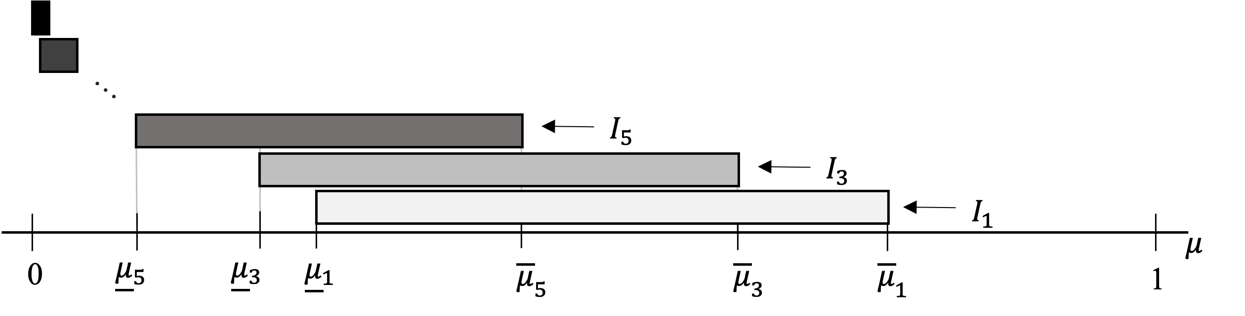
First, for any batch size $K,$ let

$${\mathcal{I}_{K}\triangleq\left(1-\mathbb{P}\left(X_{K}\geq\frac{K+1}{2}\right),\frac{q^{2}\left(1-\mathbb{P}\left(X_{K}\geq\frac{K+1}{2}\right)\right)}{q^{2}\left(1-\mathbb{P}\left(X_{K}\geq\frac{K+1}{2}\right)\right)+(1-q)^{2}\mathbb{P}\left(X_{K}\geq\frac{K+1}{2}\right)}\right)}$$

be some interval of prior where ${X_{K}\sim\text{Binomial}(K,q)}.$ Moreover, let $\overline{K}(\mu)$ (respectively, $\underline{K}(\mu)$) be the maximum (respectively, minimum) batch size $K$ such that $\mu\in\mathcal{I}_{K}.$ Then the incentive compatibility of $V_{\{K\}}$ can be characterized in terms of the interval $\mathcal{I}_{K},$ or equivalently, the batch size bounds $\overline{K}(\mu)$ and $\underline{K}(\mu)$:

Lemma 1.

$V_{\{K\}}$ is incentive-compatible if and only if (i) $\mu\in\mathcal{I}_{K}$, or equivalently (ii) $\mu<q$ and $\underline{K}(\mu)\leq K\leq\overline{K}(\mu).$

The proof of the lemma can be found in Appendix D together with the rest of the proofs in this section. A sketch of the proof is as follows. To show condition (i), for a fixed $K$, let $\mathcal{G}_{K}$ (respectively, $\mathcal{B}_{K}$) be the probability that the object gets allocated to some agent in the batch conditional on the true quality being good (respectively, bad). We compute that

$\displaystyle{\mathcal{G}_{K}=\sum_{y=\frac{K+1}{2}}^{K}\frac{1}{y}{K-1\choose y-1}q^{y-1}(1-q)^{K-y}}$ $\displaystyle\qquad{\mathcal{B}_{K}=\sum_{y=\frac{K+1}{2}}^{K}\frac{1}{y}{K-1\choose y-1}q^{K-y}(1-q)^{y-1}.}$

Next, we use $\mathcal{G}_{K}$ and $\mathcal{B}_{K}$ to rewrite the incentive compatibility constraints as ${\mu q\mathcal{G}_{K}-(1-\mu)(1-q)\mathcal{B}_{K}\geq 0}$ and ${\mu(1-q)\mathcal{G}_{K}-(1-\mu)q\mathcal{B}_{K}\leq 0.}$ Given that the left-hand sides of both inequalities monotonically increase with $\mu,$ there exist some thresholds of prior, namely $\underline{\mu}_{K}\in(0,1)$ and $\overline{\mu}_{K}\in(0,1)$, that solve the indifference conditions: $\frac{\underline{\mu}_{K}}{1-\underline{\mu}_{K}}=\frac{1-q}{q}\frac{\mathcal{B}_{K}}{\mathcal{G}_{K}}$ and $\frac{\overline{\mu}_{K}}{1-\overline{\mu}_{K}}=\frac{q}{1-q}\frac{\mathcal{B}_{K}}{\mathcal{G}_{K}}.$ Based on this transformed system of equations, we are able to characterize the feasible region $(\underline{\mu}_{K},\overline{\mu}_{K})$ for the prior $\mu$ which turns out to be precisely $\mathcal{I}_{K}$. To show the equivalent condition (ii), we utilize some useful properties of the interval $\mathcal{I}_{K}$: first, its endpoints are weakly decreasing in $K$ (Lemma 1), and second, it is overlapping (i.e., $\mathcal{I}_{K}\cap\mathcal{I}_{K+2}\neq\phi$) (Lemma 2).

Refer to caption
Figure 2: Interval of incentive-compatible prior $\mathcal{I}_{K}$ for different batch sizes $K\in\{1,3,\ldots\}$ as described in Lemma 1. The intervals $\mathcal{I}_{K}$ are decreasing (Lemma 1) with $K$ and the consecutive intervals $\mathcal{I}_{K}$ and $\mathcal{I}_{K+2}$ overlap (Lemma 2) with each other.

Condition (ii) in terms of batch size $K$ provides a straightforward intuition. Larger batch sizes make agents more confident that, if the object is allocated, it is likely that the quality is good. For the same reason, however, a batch size that is too large incentivizes everyone to opt in, including those with negative signals. Borrowing the terminology from the voting literature, $\overline{K}(\mu)$ is designed to make each agent’s decision pivotal: $\overline{K}(\mu)$ is the maximum batch size that guarantees incentive compatibility. On the other hand, if the batch size is too small, then the allocation decision depends on learning from a sample size that is too small to offer reliable information, making agents with positive signals reluctant to opt in. Thus, $\underline{K}(\mu)$ is the minimum batch size that ensures incentive compatibility. Furthermore, Lemma 1 gives rise to the following observation.

Lemma 2.

Suppose $\mu<q.$ Then, an incentive-compatible $V_{\{K\}}$ always exists and achieves correctness $c\left(V_{\{K\}}\right)=\mathbb{P}\left(X_{K}\geq\frac{K+1}{2}\right),$ where $X_{K}\sim\textrm{Binomial}(K,q).$

Lemma 2 shows that if each signal is at least as informative as the prior $\mu$, there is a single-batch voting mechanism that elicits information in a truthful manner. Another implication of the lemma is that the correctness of an incentive-compatible $V_{\{K\}}$ can be expressed as the tail distribution of a $\textrm{Binomial}(K,q)$ random variable. This tail distribution can be interpreted as the probability that the majority of votes are aligned with the true quality. Given the definition of correctness, this property is thus particularly intuitive.

An additional observation is that the tail distribution $\mathbb{P}\left(X_{K}\geq\frac{K+1}{2}\right)$ increases with $K$ (see Lemma 2 in Appendix E). Consequently, given $\mu,$ the upper size limit $\overline{K}(\mu)$ maximizes correctness among all possible values of $K$ that conserve the incentive compatibility of $V_{\{K\}}.$ We formalize this property below.

Proposition 2.

Suppose $\mu<q.$ Then the batch size $K=\overline{K}(\mu)$ maximizes correctness among all incentive-compatible $V_{\{K\}}.$

Hence the planner will choose the largest batch size that the agents’ incentives allow. As we establish below, the optimal batch size behaves monotonically with respect to the prior $\mu.$

Lemma 3.

$\overline{K}(\mu)$ weakly decreases with $\mu.$

The logic here is simple. If the sentiment around the object quality is optimistic (i.e., $\mu$ is high), then it is harder to keep the agents with negative signals truthful, requiring a tighter upper bound on the batch size (lower $\overline{K}(\mu)$). We discuss additional comparative statics through simulations in Section 5.

Finally, note that the results above focused on regimes where $\mu<q$. This a natural setting which guarantees that the signal is at least as informative as the prior belief. For the complementary case where $\mu\geq q$, we show that there is no incentive-compatible voting mechanism (see Lemma 3 in Appendix D). Intuitively, the lack of informativeness of the signal induces the agents to lose trust in their private signals, and as a result creates no incentives to behave truthfully. In that case, under any $V_{\{K\}},$ all agents will opt in and thus the object will always be allocated. Notice that this outcome is equivalent to the outcome under $V_{\textsc{seq}}$ in terms of correctness.555The only difference is that under $V_{\{K\}},$ the object is always allocated to an agent in the batch uniformly at random, whereas under $V_{\textsc{seq}}$ it is always allocated to agent $1$.

4.2 Improving Correctness via Greedy Voting Mechanisms

Next we utilize the results of Section 4.1 to characterize how to dynamically choose batch sizes of a voting mechanism (potentially with multiple batches) to improve correctness, while balancing the agents’ incentives. Further, we implement this mechanism via a simple greedy algorithm.

The first key technical observation is that, from the perspective of the agents in batch $j,$ the voting mechanism $V_{\{\pi_{j}\}_{j=1}^{\infty}}$ is equivalent to a single-batch voting mechanism $V_{\{K_{j}\}}$ with realized common belief $\mu_{j-1}$ and batch size $K_{j}=\pi_{j}\left(\mu_{j-1}\right).$ Naturally, since both the planner and agents observe the voting results from previous batches, no informational asymmetry arises between them.

Lemma 4.

A voting mechanism $V_{\{\pi_{j}\}_{j=1}^{\infty}}$ is incentive-compatible if and only if for any batch $j,$ current belief $\mu_{j-1}$ and batch size $K_{j}\triangleq\pi_{j}\left(\mu_{j-1}\right),$ $V_{\{K_{j}\}}$ is incentive-compatible.

Hence, to ensure the incentive compatibility of $V_{\{\pi_{j}\}_{j=1}^{\infty}},$ it is sufficient to choose each batch size $K_{j}$ myopically by solving a single-batch voting mechanism design problem (with updated belief $\mu_{j-1}$ instead of $\mu$). This suggests the following greedy scheme.

Definition 2.

For any $J\in\mathbb{N},$ let $V_{\textsc{greedy}}^{J}\in\mathcal{V}$ be the voting mechanism that offers the object to $J$ batches unless either it is allocated or the list is exhausted. Formally, for each batch $j$ and realized belief $\mu_{j-1},$ the batch sizes are chosen as $K_{j}=\pi_{j}(\mu_{j-1})=\footnotesize\begin{cases}\overline{K}(\mu_{j-1})&\text{ for }j\leq J\\ 0&\text{ for }j>J.\end{cases}\normalsize$

Building upon Lemma 4 and results from Section 4.1, we establish three key properties of $V_{\textsc{greedy}}^{J}$.

Proposition 3.

For any $\mu<q$ and $J,$ $V_{\textsc{greedy}}^{J}$ has the following properties:

  • (i)

    $V_{\textsc{greedy}}^{J}$ is incentive-compatible;

  • (ii)

    Ex-post batch sizes satisfy $K_{j^{\prime}}\leq K_{j}$ for any $j^{\prime}<j\in[J]$;

  • (iii)

    $c\left(V_{\textsc{greedy}}^{J}\right)$ strictly increases with $J$.

To understand part (ii), suppose that the object had been offered to batch $j$ but was not allocated. Then, the current belief naturally decreases, that is $\mu_{j}<\mu_{j-1}$, as the majority of batch $j$ has voted to opt out. By Lemma 3, a more pessimistic belief about the object quality results in a larger optimal batch size $\overline{K}(\cdot).$ Hence, it follows that $\overline{K}(\mu_{j-1})\leq\overline{K}(\mu_{j}).$ Part (iii) of the proposition suggests that adding an additional batch improves correctness. The intuition is that an additional batch allows the planner to collect and learn from more information about the object. Consequently, the planner would like to keep on offering until either the object is allocated or there are not enough agents left in the queue. We formally define this mechanism below and describe a simple algorithm to implement it.

Definition 3.

Let $V_{\textsc{greedy}}\in\mathcal{V}$ be the greedy voting mechanism such that for each batch $j$ and the realized belief $\mu_{j-1},$ the batch sizes are chosen as $K_{j}=\pi_{j}(\mu_{j-1})=\overline{K}(\mu_{j-1}).$

Initialize batch $j=1,$ belief $\mu_{0}=\mu,$ batch size $K_{1}=\overline{K}(\mu_{0})$;
while $I\geq K_{1}+\ldots+K_{j}$ do
       Collect votes from the top $K_{j}$ remaining agents;
       if $Y_{j}\geq\lceil\frac{K_{j}}{2}\rceil$ then
             Allocate the object uniformly at random among agents in batch $j$ who opted in;
            
      else
             Update belief $\mu_{j}$ using Equation (1) and next batch size $K_{j+1}=\overline{K}(\mu_{j})$;
             Set $j\leftarrow j+1$;
            
Algorithm 1 Implementation of $V_{\textsc{greedy}}$

Note that a major advantage of $V_{\textsc{greedy}}$ is its design simplicity: the maximum number of batches, $J,$ does not have to be predefined.

Finally, we are ready to prove Theorem 1. The main idea is that using the correctness $c(V_{\textsc{seq}})$ of the sequential offering mechanism from Proposition 1, we can show that for every $\mu<q,$ the planner can achieve $c\left(V_{\textsc{greedy}}^{J}\right)$ that exceeds $c(V_{\textsc{seq}}),$ by appropriately setting $J$ (full proof in Appendix D.3). Furthermore, using Proposition 3 (part (iii)), we establish that the improvement described in Theorem 1 can be also achieved by $V_{\textsc{greedy}}.$

Corollary 1.

For any $\mu<q,$ $V_{\textsc{greedy}}$ is an incentive-compatible (multi-batch) voting mechanism that improves correctness in comparison to the sequential offering mechanism $V_{\textsc{seq}}$.

5 Simulations

In this section we use simulations to complement our theoretical results.

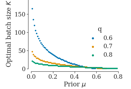
Optimal batch size. In Figure 3, we study the optimal batch size $\overline{K}(\mu)$ (Proposition 2) of the single-batch voting mechanism $V_{\{K\}}$; by construction, the optimal $V_{\{K\}}$ is equivalent to $V_{\textsc{greedy}}^{1}.$ In our numerical analysis, we examine $\overline{K}(\mu)$ for all priors $\mu\in(0,1)$ and signal precision ${q\in\{0.6,0.7,0.8\}.}$

We make several observations. First, as guaranteed by Lemma 3, the optimal batch size $\overline{K}(\mu)$ decreases as the prior $\mu$ increases. As we discussed in greater detail in Section 4.1, the incentive compatibility constraint binds at lower values of $\overline{K}(\mu).$ For very high values of $\mu$, that is $\mu\geq q$, Theorem 1 establishes that it is impossible to achieve incentive compatibility for any batch size, which explains the discontinuity at $\mu=q$ in each curve.

Second, for lower values of $\mu$ (approximately for values $\mu<0.5$), the marginal effect of $q$ on $\overline{K}(\mu)$ is negative but diminishes as $\mu$ grows. Indeed, as Figure 3 illustrates, the signal precision $q$ plays an important role for lower values of $\mu$. In particular, if $\mu$ is low and $q$ is not significantly informative (e.g., $q=0.6$), the planner has a priori low confidence in the object’s quality. Similarly, agents have strong incentives to opt out regardless of their signal. Thus, the planner needs a larger batch size.

Refer to caption
Figure 3: Via simulations, we compute the optimal incentive-compatible batch size $\overline{K}(\mu)$ for all possible priors $\mu\in(0,1)$ for three regimes: $q\in\{0.6,0.7,0.8\}$. In all regimes, $\overline{K}(\mu)$ decreases as $\mu$ increases. For low values of $\mu$, higher $q$ implies lower $\overline{K}(\mu)$.
Refer to caption
Figure 4: We compare the correctness $c(V)$ of mechanisms ${V\in\{V_{\textsc{greedy}}^{1},V_{\textsc{greedy}}^{2},V_{\textsc{seq}},V_{\textsc{all}}\}}$ in a setting with population size $I=345.$ $V_{\textsc{all}}$ represents the optimal mechanism in the absence of strategic incentives, which achieves near perfect correctness close to $1$ (see Equation (2)). The remaining $V_{\textsc{greedy}}^{1}$, $V_{\textsc{greedy}}^{2}$, and $V_{\textsc{seq}}$ assume strategic agents. We compute $c(V)$ for all $\mu\in(0,1)$ and three different regimes $q\in\{0.6,0.7,0.8\}.$ In all regimes, $V_{\textsc{greedy}}^{1}$ achieves higher correctness than $V_{\textsc{seq}}$ for all $\mu<{q}/{2}+{1}/{4}$. With one additional batch, $V_{\textsc{greedy}}^{2}$ further improves the correctness of $V_{\textsc{greedy}}^{1}$ and outperforms $V_{\textsc{seq}}$ for all $\mu<q$.

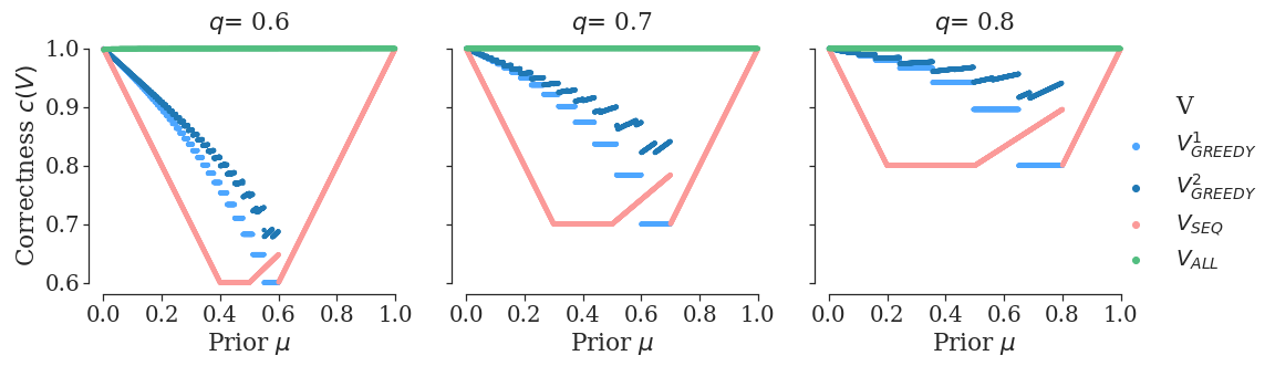
Correctness evaluation and comparison. In Figure 4, we evaluate the correctness $c(V)$ of four different mechanisms $V\in\{V_{\textsc{greedy}}^{1},V_{\textsc{greedy}}^{2},V_{\textsc{seq}},V_{\textsc{all}}\}$ for $q\in\{0.6,0.7,0.8\}$ and $\mu\in(0,1)$. For $q\in\{0.6,0.7,0.8\}$, we study the behavior of $c(V^{J}_{\textsc{greedy}})$, $J\in\{1,2\}$, as a function of the prior $\mu$. We observe several interesting properties. First, $\mu$ and $q$ apply two opposite forces on correctness: for both $J\in\{1,2\}$, $c(V^{J}_{\textsc{opt}})$ tends to decrease as $\mu$ increases but for higher $q$’s this effect is smaller. Intuitively, as the prior $\mu$ grows, the batch size becomes smaller (see Figure 3). As the planner learns from fewer signals, the probability to misallocate the object increases. However, as the signal precision $q$ improves, the magnitude of a misallocation decreases since signals become more reliable.

Second, the comparison between $V_{\textsc{greedy}}^{1}$ and $V_{\textsc{greedy}}^{2}$ confirms that an additional batch has an important positive effect on correctness. The two-batch mechanism $V_{\textsc{greedy}}^{2}$ outperforms the single-batch mechanism $V_{\textsc{greedy}}^{1}$. In fact, the gap between their achieved correctness grows as $\mu$ increases. Intuitively, if the planner fails to allocate a good object in the first batch, she has another chance to allocate it in the second batch. Since a higher $\mu$ translates to a higher probability that the object is of good quality, having two opportunities to allocate the object has a positive impact on correctness. This also explains the non-monotonic (but still generally decreasing) trend of $c(V_{\textsc{greedy}}^{2})$ with respect to $\mu$, which is especially evident for high values of $\mu.$

Finally, we are interested in comparing the correctness of voting mechanisms against two natural benchmarks. The first benchmark $V_{\textsc{seq}}$ is the sequential offering mechanism (see Section 3) in the presence of strategic incentives. As established in Theorem 1, there exists a voting mechanism (in this case, $V_{\textsc{greedy}}^{2}$) which outperforms $V_{\textsc{seq}}$ for all $\mu<q$. However, observe that the number of batches is crucial. In contrast to $V_{\textsc{greedy}}^{2}$, $V_{\textsc{greedy}}^{1}$ achieves higher correctness than $V_{\textsc{seq}}$ only for $\mu<\frac{q}{2}+\frac{1}{4}$.

Comparing $V_{\textsc{greedy}}^{2}$ against $V_{\textsc{seq}}$, we observe that the performance gap $c(V_{\textsc{greedy}}^{2})-c(V_{\textsc{seq}})$ widens in the region $\mu\in[0,1-q]$ as $\mu$ grows. This is because the object is always discarded for $\mu<q$ (see Figure 1) which further explains why $c(V_{\textsc{seq}})=1-\mu$ (Proposition 1). For $\mu\in(1-q,q)$, the gap remains positive but decreases as $\mu$ increases, since the signals of the first two agents affect the outcome of $V_{\textsc{seq}}$ and thus decrease the chance of misallocation. Note again that, due to Theorem 1, for $\mu\geq q$, any voting mechanism $V\in\mathcal{V}$ achieves correctness equal to $c(V_{\textsc{seq}})$.

The second benchmark $V_{\textsc{all}}$ assumes that agents are not strategic (see Equation (2)) and thus achieves the optimal correctness close to 1. The ratio $c(V^{J}_{\textsc{greedy}})/c(V_{\textsc{seq}})$, $J\in\{1,2\}$, serves as a measure of the price of anarchy. We see that incentives put a significant cost on correctness, especially for higher values of $\mu\leq q$. Higher values of $q$ help decrease the price of anarchy. For any $q$, the maximum price of anarchy $c(V^{J}_{\textsc{greedy}})/c(V_{\textsc{seq}})$ is observed around $\mu=q,$ and equals $1/q$ in a single-batch mechanism.

6 Discussion and Conclusion

Recent empirical evidence suggests that a significant contributing factor to the high discard rate of donated organs is herding. We propose to amend the current allocation policy by incorporating learning and randomness into the allocation process. We support our recommendations by introducing and analyzing a stylized model through theory and simulations. From a theoretical perspective, our work highlights the tension between learning and incentives and contributes to the understanding of optimal allocation when agents are privately informed and thus susceptible to herding behavior.

Limitations and extensions. For simplicity, we make two limiting assumptions: (1) agent utilities are symmetric; (2) agents differ only in the realization of their private signals. We believe that our results are qualitatively robust and can be extended to a model with variations in agent types and asymmetric utilities. Increasing the relative magnitude of accepting a “bad” object will make agents more cautious, thus leading to larger batches. Introducing heterogeneous agents adds little insight to our qualitative conclusions; therefore, for the sake of brevity, we considered homogeneous agents.

Nevertheless, we acknowledge that our model is stylized with several abstractions that may not fully reflect the real organ allocation markets. In practice, an organ allocation waitlist might have patients of varying medical characteristics, such as age and blood type, which can give rise to heterogeneous utilities from the same organ. Therefore, our current model, which assumes a common utility function, should be interpreted as restricting attention to patients within the same medical characteristics group. It would be an interesting future direction to generalize some of these parts of our model.

Social impact and ethical concerns. Our proposed mechanism is designed to increase the acceptance rate of transplantable donated organs. While designing healthcare policies using insights from theoretical models has been extensively used (see e.g., [5, 4] for kidney exchange), we emphasize that one must pursue such a change in a gradual manner. Furthermore, we note that our mechanism does not constitute a Pareto improvement. Patients, who are first in line, may be skipped due to the randomness in allocation. Thus, although our policy has the potential to improve the overall system efficiency, its implementation must consider any unintended effects on individual patients.

Acknowledgments and Disclosure of Funding

Jamie Kang acknowledges support of the Jerome Kaseberg Doolan Fellowship and Stanford Management Science & Engineering Graduate Fellowship.

Faidra Monachou acknowledges support from the Stanford Data Science Scholarship, Google Women Techmakers Scholarship, Stanford McCoy Family Center for Ethics in Society Graduate Fellowship, Jerome Kaseberg Doolan Fellowship, and A.G. Leventis Foundation Grant.

Moran Koren acknowledges the support of the Israeli Minestry of Science and Technologi’s Shamir scholarship and the support of the Fulbright foundation.

References

  • Acemoglu et al. [2010] Daron Acemoglu, Asuman Ozdaglar, and Ali Parandehgheibi. Spread of Misinformation in Social Networks. Games and Economic Behavior, 2010.
  • Arieli and Mueller-Frank [2019] Itai Arieli and Manuel Mueller-Frank. Multidimensional Social Learning. The Review of Economic Studies, 86(3):913–940, may 2019. doi: 10.1093/restud/rdy029. URL https://academic.oup.com/restud/article/86/3/913/5034182.
  • Arieli et al. [2018] Itai Arieli, Moran Koren, and Rann Smorodinsky. The One-Shot Crowdfunding Game. In EC ’18: Proceedings of the 2018 ACM Conference on Economics and Computation, pages 213–214. ACM, 2018.
  • Ashlagi and Roth [2014] Itai Ashlagi and Alvin E Roth. Free Riding and Participation in Large Scale, Multi-hospital Kidney Exchange. Theoretical Economics, 9(3):817–863, 2014.
  • Ashlagi and Roth [2021] Itai Ashlagi and Alvin E Roth. Kidney Exchange: An Operations Perspective. Technical report, National Bureau of Economic Research, 2021.
  • Austen-Smith and Banks [1996] David Austen-Smith and Jeffrey S Banks. Information Aggregation, Rationality, and the Condorcet Jury Theorem. The American Political Science Review, 90(1):pp. 34–45, 1996. ISSN 00030554. URL http://www.jstor.org/stable/2082796.
  • Banerjee [1992] Abhijit V Banerjee. A Simple Model of Herd Behavior. The Quarterly Journal of Economics, 107(3):797–817, 1992.
  • Bikhchandani et al. [1992] Sushil Bikhchandani, David Hirshleifer, and Ivo Welch. A Theory of Fads, Fashion, Custom, and Cultural Change as Informational Cascades. Journal of Political Economy, 100(5):992–1026, 1992.
  • Butler et al. [2020] Alison Butler, Gretchen Chapman, Jonathan N Johnson, Antonio Amodeo, Jens Böhmer, Manuela Camino, Ryan R Davies, Anne I Dipchand, Justin Godown, Oliver Miera, et al. Behavioral economics—a framework for donor organ decision-making in pediatric heart transplantation. Pediatric transplantation, 24(3):e13655, 2020.
  • Che and Horner [2015] Yeon-Koo Che and Johannes Horner. Optimal Design for Social Learning. 2015.
  • Cooper et al. [2019] Matthew Cooper, Richard Formica, John Friedewald, Ryutaro Hirose, Kevin O’Connor, Sumit Mohan, Jesse Schold, David Axelrod, and Stephen Pastan. Report of National Kidney Foundation Consensus Conference to Decrease Kidney Discards. Clinical Transplantation, 33(1):e13419, 2019.
  • De Condorcet [1785] Nicolas De Condorcet. Essay sur l’application de l’analyse a la probabilite des decisions rendues a la pluralite des voix. Par m. le marquis De Condorcet.. de l’imprimerie royale, 1785.
  • De Mel et al. [2020] Stephanie De Mel, Kaivan Munshi, Soenje Reiche, and Hamid Sabourian. Herding in Quality Assessment: An Application to Organ Transplantation. Technical report, IFS Working Papers, 2020.
  • Eyster et al. [2013] Erik Eyster, Andrea Galeotti, Navin Kartik, and Matthew Rabin. Congested Observational Learning. Games and Economic Behavior, 87(283454):1–32, 2013. doi: 10.1016/j.geb.2014.06.006. URL http://dx.doi.org/10.1016/j.geb.2014.06.006.
  • Glazer et al. [2021] Jacob Glazer, Ilan Kremer, and Motty Perry. The Wisdom of the Crowd When Acquiring Information Is Costly. Management Science, 2021.
  • Immorlica et al. [2018] Nicole Immorlica, Jieming Mao, Aleksandrs Slivkins, and Zhiwei Steven Wu. Incentivizing Exploration with Unbiased Histories. arXiv preprint arXiv:1811.06026, 2018.
  • Immorlica et al. [2019] Nicole Immorlica, Jieming Mao, Aleksandrs Slivkins, and Zhiwei Steven Wu. Bayesian Exploration with Heterogeneous Agents. In The World Wide Web Conference, pages 751–761. ACM, 2019.
  • Kamenica and Gentzkow [2011] Emir Kamenica and Matthew Gentzkow. Bayesian Persuasion. American Economic Review, 101(6):2590–2615, 2011.
  • Kolotilin et al. [2017] Anton Kolotilin, Tymofiy Mylovanov, Andriy Zapechelnyuk, and Ming Li. Persuasion of a Privately Informed Receiver. Econometrica, 85(6):1949–1964, 2017.
  • Kremer et al. [2014] Ilan Kremer, Yishay Mansour, and Motty Perry. Implementing the “Wisdom of the Crowd”. Journal of Political Economy, 122(5):988–1012, 2014.
  • Mankowski et al. [2019] Michal A Mankowski, Martin Kosztowski, Subramanian Raghavan, Jacqueline M Garonzik-Wang, David Axelrod, Dorry L Segev, and Sommer E Gentry. Accelerating kidney allocation: Simultaneously expiring offers. American Journal of Transplantation, 19(11):3071–3078, 2019.
  • Mansour et al. [2016] Yishay Mansour, Aleksandrs Slivkins, Vasilis Syrgkanis, and Zhiwei Steven Wu. Bayesian Exploration: Incentivizing Exploration in Bayesian Games. arXiv preprint arXiv:1602.07570, 2016.
  • Mohan et al. [2018] Sumit Mohan, Mariana C Chiles, Rachel E Patzer, Stephen O Pastan, S Ali Husain, Dustin J Carpenter, Geoffrey K Dube, R John Crew, Lloyd E Ratner, and David J Cohen. Factors Leading to the Discard of Deceased Donor Kidneys in the United States. Kidney International, 94(1):187–198, 2018.
  • Mossel et al. [2015] Elchanan Mossel, Allan Sly, and Omer Tamuz. Strategic Learning and the Topology of Social Networks. Econometrica, 83(5):1755–1794, 2015. doi: 10.3982/ECTA12058. URL http://arxiv.org/abs/1209.5527.
  • National Kidney Foundation [2016] National Kidney Foundation. Organ Donation and Transplantation Statistics, January 2016. URL https://www.kidney.org/news/newsroom/factsheets/Organ-Donation-and-Transplantation-Stats.
  • Papanastasiou et al. [2017] Yiangos Papanastasiou, Kostas Bimpikis, and Nicos Savva. Crowdsourcing Exploration. Management Science, 64(4):1727–1746, 2017.
  • Rayo and Segal [2010] Luis Rayo and Ilya Segal. Optimal Information Disclosure. Journal of political Economy, 118(5):949–987, 2010.
  • Smith and Sørensen [2000] Lones Smith and Peter Sørensen. Pathological Outcomes of Observational Learning. Econometrica, 68(2):371–398, 2000.
  • Stewart et al. [2017] Darren E Stewart, Victoria C Garcia, John D Rosendale, David K Klassen, and Bob J Carrico. Diagnosing the Decades-long Rise in the Deceased Donor Kidney Discard Rate in the United States. Transplantation, 101(3):575–587, 2017.
  • U.S. Department of Health and Human Services [2021] U.S. Department of Health and Human Services. Organ Procurement and Transplantation Network: National Data, April 2021. URL https://optn.transplant.hrsa.gov/data/view-data-reports/national-data/.
  • Zhang [2010] Juanjuan Zhang. The Sound of Silence: Observational Learning in the U.S. Kidney Market. Marketing Science, 29(2), 2010. doi: 10.1287/mksc.1090.0500.

Appendix A Extended Related Literature

The information structure of the model is based on the literature on observational learning. The seminal papers by [7, 8] show that if agents receive binary signals over the object’s quality and observe previous agents’ action history, herding (information cascades) will eventually take place and information will be not be aggregated. These findings are extended by [28] to general distributions and follow-up works examine the robustness of these results in various game structures [1, 14, 24, 2]. Note that none of these works consider the existence of a planner that is able to control the flow of information.

Several empirical studies examine the presence of observational learning in real-world scenarios [31, 13]. Using data from organ transplantation in the United Kingdom, [13] develop empirical tests to detect herding behavior and quantify its welfare consequences. [31] provides empirical evidence for herding behavior in the United States deceased donor waitlist. Moreover, there also have been growing clinical literature on behavioral factors in organ allocation such as [9, 11].

To improve the performance of the allocation system, we propose utilizing a voting mechanism to elicit agents private information. The ability of voting procedures to uncover ground truth by aggregating dispersed information dates back to the seminal Condorcet Jury Theorem [12], which utilizes the law of large numbers to assert that majority voting will reach the correct decision, provided that the population is large enough and agents are not strategic. [6] show that Condorcet’s result does not hold when agents are strategic and are allowed to deviate from their private information. Our notion of correctness is taken from [3]. One novel feature in our model is that the number of votes is determined endogenously to maximize the probability of making the correct choice.

Our work is also loosely connected to the literature on information design (e.g., [18, 19, 27, 26, 10]) and Bayesian exploration (e.g., [20, 15, 16, 22, 17]). With the exception of [15], who consider an online recommendation problem with costly information acquisition, most of these works do not take into account the possibility that agents are privately informed. Instead, several papers such as [19, 17] consider agents with private information in the form of types or idiosyncratic preferences. In contrast to our model where private signals are informative about the true quality of the object, those types are not correlated with the true state variable.666I.e., in our case, knowing the value of private signals does lead the decision maker to update her belief accordingly to this information.

Appendix B Optimal Solution in the Absence of Strategic Incentives

Lemma 1.

Suppose that agents are not strategic and voluntarily reveal their private signal value to the planner. Let

$$\underline{y}=0.5\,\frac{\log\left(\frac{1-\mu}{\mu}\right)}{\log\left(\frac{q}{1-q}\right)}+0.5\,I.$$

Then, the planner achieves optimal correctness when she allocates the object if and only if $\sum_{i=1}^{I}\mathbf{1}\{s_{i}=g\}\geq\underline{y}$.

Proof.

Conditional on $\omega=G$, the number $X_{G}$ of positive signals $s=g$ follows a binomial distribution, i.e., $X_{G}\sim\textrm{Binomial}(I,q)$. Conditional on $\omega=G$, the number $X_{B}$ of positive signals $s=g$ follows a binomial distribution, i.e., $X_{B}\sim\textrm{Binomial}(I,1-q)$.

Let $\underline{y}$ denote the number of minimal positive signals required to allocate the object. For any number of positive signals higher than $\underline{y}$, it is also optimal to allocate the object since the posterior belief that $\omega=G$ strictly increases.

The threshold $\underline{y}$ is the smallest integer that satisfies

$$\begin{split}&\mathbb{P}(\omega=G\mid X_{G}=\underline{y})\geq 0.5\\ \iff&\frac{\mu{I\choose\underline{y}}q^{\underline{y}}(1-q)^{I-\underline{y}}}{\mu{I\choose\underline{y}}q^{\underline{y}}(1-q)^{I-\underline{y}}+(1-\mu){I\choose\underline{y}}q^{I-\underline{y}}(1-q)^{\underline{y}}}\geq 0.5\\ \iff&\mu q^{\underline{y}}(1-q)^{I-\underline{y}}\geq(1-\mu)q^{I-\underline{y}}(1-q)^{\underline{y}}\\ \iff&\mu q^{2\underline{y}-I}\geq(1-\mu)(1-q)^{2\underline{y}-I}\\ \iff&\left(\frac{q}{1-q}\right)^{2\underline{y}-I}\geq\frac{1-\mu}{\mu}.\end{split}$$

Recall that $q\in(0.5,1)$. Taking the logarithm of the previous relation and rearranging the terms, we finally get that

$$\underline{y}=0.5\,\frac{\log\left(\frac{1-\mu}{\mu}\right)}{\log\left(\frac{q}{1-q}\right)}+0.5\,I.$$

Appendix C Omitted Analysis of the Sequential Offering Mechanism (Section 3)

We first analyze the optimal strategies of the first three agents in the queue. Before taking any action, each agent observes his position in the queue in addition to his private signal and the common object prior $\mu$. In particular, by observing his position $i$, agent $i$ recognizes that the object is being offered to him because all of the $i-1$ preceding agents have rejected it. This observation contributes to his posterior belief about the object quality.

Agent $1$. Agent $1$ updates his posterior belief using Bayes’ law based only on his signal $s_{1}.$

$\displaystyle\mathbb{P}(\omega=G|s_{1})=\begin{cases}\frac{\mu q}{\mu q+(1-\mu)(1-q)}&\text{ for }s_{1}=g\\ \frac{\mu(1-q)}{\mu(1-q)+(1-\mu)q}&\text{ for }s_{1}=b.\end{cases}$

Since he receives utility $1$ if $\omega=G$ and $-1$ if $\omega=B,$ his expected utility to opt in is ${\mathbb{P}(\omega=G|s_{1})-\left(1-\mathbb{P}(\omega=G|s_{1})\right).}$ On the other hand, his utility to opt out is $0.$ We observe that agent $1$ is better off opting in if

$$\mathbb{P}(\omega=G|s_{1})-\left(1-\mathbb{P}(\omega=G|s_{1})\right)>0,$$

which corresponds to

$\displaystyle\begin{cases}\mu q-(1-\mu)(1-q)>0&\text{ when }s_{1}=g,\\ \mu(1-q)-(1-\mu)q>0&\text{ when }s_{1}=b.\end{cases}.$

Let $\alpha_{1}$ be agent $1$’s optimal action in this mechanism. Then the following lemma characterizes $\alpha_{1}$.

Lemma 1.

Under the sequential offering mechanism, agent $1$ chooses action

$\displaystyle\alpha_{1}=\begin{cases}y&\text{ for }\mu>q\\ \mathbb{I}\{s_{1}=g\}&\text{ for }\mu\in(1-q,q]\\ n&\text{ for }\mu\leq 1-q.\end{cases}$

Lemma 1 shows that the sequential offering mechanism drives the first agent to follow his signal if it is more informative than the common prior (i.e., when $\mu\in(1-q,q]$). In the opposite case, where the prior is more informative (i.e., when either $\mu>q$ or $\mu\leq 1-q$), the agent ignores his private signal. In particular, for high priors $\mu>q$ the object is always allocated to agent $1$ regardless of its true quality $\omega$.

Agent $2$. When the second agent is offered the object, he knows that the first agent has already opted out. At the same time, agent 2 is aware of agent 1’s optimal strategy as described in Lemma 1. Therefore, if the prior satisfies $\mu\in(1-q,q],$ then agent 2 infers that agent 1 has followed his own signal $s_{1}=b.$ As such, for $\mu\in(1-q,q]$, agent 2 updates his posterior belief informed by this observation as follows:

$\displaystyle\mathbb{P}(\omega=G|s_{2},\alpha_{1}=n)=\begin{cases}\mu&\text{ for }\mu\in(1-q,q],s_{2}=g\\ \frac{\mu(1-q)^{2}}{\mu(1-q)^{2}+(1-\mu)q^{2}}&\text{ for }\mu\in(1-q,q],s_{2}=b.\end{cases}$

On the other hand, for $\mu\notin(1-q,q]$, it holds that

$\displaystyle\mathbb{P}(\omega=G|s_{2},\alpha_{1}=n)=\begin{cases}\frac{\mu q}{\mu q+(1-\mu)(1-q)}&\text{ for }\mu\notin(1-q,q],s_{2}=g\\ \frac{\mu(1-q)}{\mu(1-q)+(1-\mu)q}&\text{ for }\mu\notin(1-q,q],s_{2}=b,\end{cases}$

in which case agent 1’s action is uninformative to agent 2.

Lemma 2.

Under the sequential offering mechanism, agent $2$ chooses777In the sequential offering mechanism, if $\mu>q$ then the object is never offered to agent $i\geq 2,$ because agent 1 always opts in.

$\displaystyle\alpha_{2}=\begin{cases}\mathbb{I}\{s_{2}=g\}&\text{ for }\mu\in(1/2,q]\\ n&\text{ for }\mu\leq 1/2.\end{cases}$
Proof.

Similarly to agent 1, agent 2 prefers to opt in if

$\displaystyle\mathbb{P}(\omega=G|s_{2},\alpha_{1}=n)-(1-\mathbb{P}(\omega=G|s_{2},\alpha_{1}=n))>0.$ (3)

For $\mu\in(1-q,q]$ and $s_{2}=g,$ Equation (3) holds when $\mu>1/2.$ For $\mu\in(1-q,q]$ and $s_{2}=b,$ Equation (3) corresponds to

$\displaystyle\mu(1-q)^{2}-(1-\mu)q^{2}>0.$

However, for any $\mu\in(1-q,q]$ we have

$\displaystyle\mu(1-q)^{2}-(1-\mu)q^{2}\leq q(1-q)^{2}-(1-q)q^{2}=q(1-q)\left(1-2q\right)<0,$

which makes Equation (3) infeasible.

For $\mu\leq 1-q,$ notice that

$\displaystyle\mu(1-q)-(1-\mu)q<\mu q-(1-\mu)(1-q)\leq 0.$

Thus Equation (3) is again infeasible regardless of $s_{2}.$

For $\mu=1/2$ exactly, by our assumption, he simply rejects the object. Therefore, agent 2 prefers to opt in if $\mu\in(1/2,q]$ and $s_{2}=g.$ Otherwise, he prefers to opt out. ∎

Lemma 2 shows that agent 2 follows his signal if $\mu>1/2,$ whereas he ignores the signal and opts out if $\mu\leq 1/2.$ The characterizations of $\alpha_{1}$ and $\alpha_{2}$ offer implications that will be useful to analyze the optimal strategies of subsequent agents. First, for $\mu>1/2$, Lemma 1 and Lemma 2 together suggest that both agent 1 and agent 2 follow their signals. Therefore, the availability of the object after being offered to agent 2 implies to subsequent agents that both ${s_{1}=b}$ and ${s_{2}=b.}$ Second, for $\mu\leq 1/2,$ agent 2’s action is uninformative about $s_{2}$. Agent 1’s action, however, can be informative depending on the value of $\mu.$ If $\mu\in(1-q,1/2)$ then the subsequent agents can infer that $s_{1}=b$ because agent 1 follows his signal. If $\mu\leq 1-q,$ however, agent 1’s action is also uninformative.

Notice here that, whenever agent $1$’s or $2$’s opt-out action is informative, his private signal (that the subsequent agents can perfectly infer) is $b.$ We use this implication for our analysis next.

Agent $3$. If the object is offered to agent 3, one of the three events must have occurred: (i) $\mu\in(1/2,q]$ and $s_{1}=s_{2}=b$, or (ii) $\mu\in(1-q,1/2]$ and $s_{1}=b$, or (iii) $\mu\leq 1-q.$ Nonetheless, we claim that in any case, agent 3 would always choose to opt out.

Lemma 3.

Under the sequential offering mechanism, agent 3 always chooses to opt out: $\alpha_{3}=n.$

Proof.

Agent 3 will prefer to opt in if

$\displaystyle\mathbb{P}(\omega=G|s_{3},\alpha_{1}=\alpha_{2}=n)-(1-\mathbb{P}(\omega=G|s_{3},\alpha_{1}=\alpha_{2}=n))>0.$ (4)

For $\mu\in(1/2,q],$ agent 3’s posterior belief given her signal is

$\displaystyle\mathbb{P}(\omega=G|s_{3},\alpha_{1}=\alpha_{2}=n)$ $\displaystyle=\mathbb{P}(\omega=G|s_{3},s_{1}=s_{2}=b)$
$\displaystyle=\begin{cases}\frac{\mu(1-q)^{2}q}{\mu(1-q)^{2}q+(1-\mu)q^{2}(1-q)}&\text{ for }\mu\in(1/2,q],s_{3}=g\\ \frac{\mu(1-q)^{3}}{\mu(1-q)^{3}+(1-\mu)q^{3}}&\text{ for }\mu\in(1/2,q],s_{3}=b\end{cases}.$

For $s_{3}=g$, we have

$\displaystyle\mu(1-q)^{2}q-(1-\mu)q^{2}(1-q)=(1-q)q[\mu(1-q)-(1-\mu)q]\leq 0.$

The proof is analogous for $s_{2}=b$. As a result, for $\mu\in(1/2,q]$ agent 3 prefers to opt out regardless of his own signal.

For $\mu\in(1-q,1/2],$ agent 3 infers that $s_{1}=b.$ Agent 3’s posterior belief equals

$\displaystyle\mathbb{P}(\omega=G|s_{3},\alpha_{1}=\alpha_{2}=n)$ $\displaystyle=\mathbb{P}(\omega=G|s_{3},s_{1}=b)$
$\displaystyle=\begin{cases}\mu&\text{ for }\mu\in(1-q,1/2],s_{3}=g\\ \frac{\mu(1-q)^{2}}{\mu(1-q)^{2}+(1-\mu)q^{2}}&\text{ for }\mu\in(1-q,1/2],s_{3}=b.\end{cases}$

Then Equation (4) is infeasible because

$$\mu-(1-\mu)=2\mu-1\leq 0.$$

Finally, for $\mu\leq 1-q,$

$\displaystyle\mathbb{P}(\omega=G|s_{3},\alpha_{1}=\alpha_{2}=n)$ $\displaystyle=\mathbb{P}(\omega=G|s_{3})$
$\displaystyle=\begin{cases}\frac{\mu q}{\mu q+(1-\mu)(1-q)}&\text{ for }\mu\leq 1-q,s_{3}=g\\ \frac{\mu(1-q)}{\mu(1-q)+(1-\mu)q}&\text{ for }\mu\leq 1-q,s_{3}=b\end{cases}$

where we have

$\displaystyle\mu(1-q)-(1-\mu)q<\mu q-(1-\mu)(1-q)=\mu+q-1\leq 0,$

making Equation (4) infeasible.

Now we extend Lemma 3 to any remaining agent in the queue. Let $\alpha_{i}$ denote the optimal action of agent $i.$

Lemma 4.

In the sequential offering mechanism, any agent other than the first two always opts-out. That is, for any $i\geq 3:$

$$\alpha_{i}=n.$$
Proof.

We use mathematical induction on $i$ to prove the statement. For the basis $i=3$, we have that due to Lemma 3 agent 3 always opts out thus his action is always uninformative to the subsequent agents. Next, as the inductive step, consider some agent $i.$ Suppose that agent $i$ updates his posterior belief in some manner such that it is optimal for him to opt out regardless of $s_{i}.$ Because this action is uninformative, the next agent $i+1$ must update his posterior belief the same way as agent $i.$ Therefore, it is also optimal for agent $i+1$ to opt out. ∎

Another way to interpret Lemma 4 is that if neither agent 1 nor agent 2 opts in, then the object will be discarded. Using this result along with Lemma 1 and Lemma 2 we characterize the outcome of the sequential offering mechanism (Lemma 1 in Section 3):

See 1

Proof.

The proof follows directly from combining Lemmas 1 to 4. ∎

See 1

Proof.

Part (i) directly follows from Lemma 1. For part (ii), notice that for $\mu\in(1/2,q],$ the object is allocated if either $s_{1}=g$ or $s_{2}=g.$ Conditional on $\omega=G,$ this happens with probability $1-(1-q)^{2}.$ The object is discarded if $s_{1}=s_{2}=b,$ which happens with $q^{2}$ conditional on $\omega=B.$ Recall that $\mathbb{P}(\omega=G)=\mu.$ Therefore the correctness of the outcome is $\mu\left(1-(1-q)^{2}\right)+(1-\mu)q^{2}=2\mu q(1-q)+q^{2}.$

For $\mu\in(1-q,1/2]$ the object is allocated if $s_{1}=g.$ Conditional on $\omega=G,$ the object is allocated with probability $q.$ The object is discarded when $s_{1}=b$ and conditional on $\omega=B$ this happens with probability $q.$ Hence the outcome is correct with probability $q.$

Appendix D Proofs for Section 4

D.1 Proofs for Section 4.1

See 1

Proof.

Proof of (i): Consider a single-batch voting mechanism $V_{\{K\}}.$ Suppose that agent $i$ chooses to opt in. Let $\mathcal{G}_{K}$ be the probability that the object gets allocated to agent $i$ conditional on the object quality being good. Similarly, let $\mathcal{B}_{K}$ be the probability that the object gets allocated to agent $i$ conditional on the object quality being bad. Then $\mathcal{G}_{K}$ and $\mathcal{B}_{K}$ can be computed as

$\displaystyle\mathcal{G}_{K}$ $\displaystyle=\sum_{y=\frac{K+1}{2}}^{K}\frac{1}{y}{K-1\choose y-1}q^{y-1}(1-q)^{K-y}$
$\displaystyle\mathcal{B}_{K}$ $\displaystyle=\sum_{y=\frac{K+1}{2}}^{K}\frac{1}{y}{K-1\choose y-1}q^{K-y}(1-q)^{y-1}.$

Given private signal $s_{i},$ his expected utility conditional on each action is

$\displaystyle u_{i}(y;s_{i})$ $\displaystyle=\mathbb{P}(\omega=G|s_{i})\mathcal{G}_{K}-\mathbb{P}(\omega=B|s_{i}=g)\mathcal{B}_{K}$
$\displaystyle u_{i}(n;s_{i})$ $\displaystyle=0.$

Then the mechanism $V_{\{K\}}$ is incentive-compatible if $u_{i}(y;g)\geq u_{i}(n;g)$ and $u_{i}(y;b)\leq u_{i}(n;b).$ That is, $V_{\{K\}}$ is incentive-compatible for prior $\mu$ if

$\displaystyle u_{i}(y;g)\geq u_{i}(n;g)$ $\displaystyle\iff\mathbb{P}(\omega=G|s_{i}=g)\mathcal{G}_{K}-\mathbb{P}(\omega=B|s_{i}=g)\mathcal{B}_{K}\geq 0$
$\displaystyle\iff\frac{\mathbb{P}(\omega=G)\mathbb{P}(s_{i}=g|\omega=G)\mathcal{G}_{K}}{\mathbb{P}(s_{i}=g)}-\frac{\mathbb{P}(\omega=B)\mathbb{P}(s_{i}=g|\omega=B)\mathcal{B}_{K}}{\mathbb{P}(s_{i}=g)}\geq 0$
$\displaystyle\iff\mu q\mathcal{G}_{K}-(1-\mu)(1-q)\mathcal{B}_{K}\geq 0$ (5)

and

$\displaystyle u_{i}(y;b)\geq u_{i}(n;b)$ $\displaystyle\iff\mathbb{P}(\omega=G|s_{i}=b)\mathcal{G}_{K}-\mathbb{P}(\omega=B|s_{i}=b)\mathcal{B}_{K}\leq 0$
$\displaystyle\iff\frac{\mathbb{P}(\omega=G)\mathbb{P}(s_{i}=b|\omega=G)\mathcal{G}_{K}}{\mathbb{P}(s_{i}=b)}-\frac{\mathbb{P}(\omega=B)\mathbb{P}(s_{i}=b|\omega=B)\mathcal{B}_{K}}{\mathbb{P}(s_{i}=b)}\leq 0$
$\displaystyle\iff\mu(1-q)\mathcal{G}_{K}-(1-\mu)q\mathcal{B}_{K}\leq 0.$ (6)

Given that the left-hand sides of both (5) and (6) monotonically increases with $\mu,$ there should be some thresholds of prior, namely $\underline{\mu}_{K}\in(0,1)$ and $\overline{\mu}_{K}\in(0,1)$, such that

$$\mu q\mathcal{G}_{K}-(1-\mu)(1-q)\mathcal{B}_{K}\geq 0\quad\forall\mu\geq\underline{\mu}_{K}$$
$$\mu(1-q)\mathcal{G}_{K}-(1-\mu)q\mathcal{B}_{K}\leq 0\quad\forall\mu\geq\overline{\mu}_{K},$$

where the thresholds solve the following indifference conditions:

$\displaystyle\frac{\underline{\mu}_{K}}{1-\underline{\mu}_{K}}$ $\displaystyle=\frac{1-q}{q}\frac{\mathcal{B}_{K}}{\mathcal{G}_{K}}$ (7)
$\displaystyle\frac{\overline{\mu}_{K}}{1-\overline{\mu}_{K}}$ $\displaystyle=\frac{q}{1-q}\frac{\mathcal{B}_{K}}{\mathcal{G}_{K}}.$ (8)

Because $q>\frac{1}{2}$ it naturally follows that $\underline{\mu}_{K}<\overline{\mu}_{K}.$ Therefore, there exists a threshold policy such that any given $V_{\{K\}}$ is incentive-compatible for a prior $\mu$ that satisfies $\underline{\mu}_{K}\leq\mu\leq\overline{\mu}_{K}.$

Next we fully characterize $\underline{\mu}_{K}$ and $\overline{\mu}_{K}.$ To do so, we use Lemma 1 to write

$$\mathcal{G}_{K}=\frac{1}{q}\cdot\frac{1}{K}\sum_{y=\frac{K+1}{2}}^{K}{K\choose y}q^{y}(1-q)^{K-y}$$
$$\mathcal{B}_{K}=\frac{1}{1-q}\cdot\frac{1}{K}\sum_{y=0}^{\frac{K+1}{2}-1}{K\choose y}q^{y}(1-q)^{K-y}$$

and therefore

$\displaystyle\frac{\mathcal{B}_{K}}{\mathcal{G}_{K}}=\frac{q}{1-q}\cdot\frac{1-\mathbb{P}\left(X_{K}\geq\frac{K+1}{2}\right)}{\mathbb{P}\left(X_{K}\geq\frac{K+1}{2}\right)}$ (9)

where $X_{K}$ is a $\text{binomial}(K,q)$ random variable. Plugging this into (7) and (8) we obtain

$\displaystyle\underline{\mu}_{K}$ $\displaystyle=1-\mathbb{P}\left(X\geq\frac{K+1}{2}\right)$ (10)
$\displaystyle\overline{\mu}_{K}$ $\displaystyle=\frac{q^{2}\left(1-\mathbb{P}\left(X\geq\frac{K+1}{2}\right)\right)}{q^{2}\left(1-\mathbb{P}\left(X\geq\frac{K+1}{2}\right)\right)+(1-q)^{2}\mathbb{P}\left(X\geq\frac{K+1}{2}\right)}$ (11)
$\displaystyle=\frac{q^{2}\underline{\mu}_{K}}{q^{2}\underline{\mu}_{K}+(1-q)^{2}(1-\underline{\mu}_{K})}.$

Letting $\mathcal{I}_{K}\triangleq\left(\underline{\mu}_{K},\overline{\mu}_{K}\right)$ concludes the proof.

Proof of (ii): By Lemmas 1 and 2 (stated below), the set of $K$ such that $\mu\in\mathcal{I}_{K}$ must be comprised of consecutive odd numbers. Therefore, for any $K$ that satisfies $\underline{K}(\mu)\leq K\leq\overline{K}(\mu),$ the corresponding $V_{\{K\}}$ must be incentive-compatible. ∎

We show two technical lemmas with regards to $\mathcal{I}_{K}$ that were used to prove Lemma 1. In doing so, we make use of Lemma 2.

Lemma 1 (Decreasing $\mathcal{I}_{K}$).

$\mathcal{I}_{K}$ decreases with $K.$ That is, the endpoints $\overline{\mu}_{K}$ and $\underline{\mu}_{K}$ both decrease with $K.$ In particular, $\overline{\mu}_{1}=q$ and $\lim_{K\rightarrow\infty}\underline{\mu}_{K}=0.$

Proof.

Recall that the endpoints $\underline{\mu}_{K}$ and $\overline{\mu}_{K}$ are computed as Equations (10), both of which by Lemma 2, decrease with $K.$ To see the second part of the statement, since

$$\mathbb{P}\left(X_{1}\geq 1\right)=\mathbb{P}\left(X_{1}=1\right)=q$$

it follows that $\overline{\mu}_{1}=\frac{q^{2}(1-q)}{q^{2}(1-q)+(1-q)^{2}q}=q.$ Moreover,

$\displaystyle\lim_{K\rightarrow\infty}\underline{\mu}_{K}=\lim_{K\rightarrow\infty}\frac{q^{2}\left(1-\mathbb{P}\left(X_{K}\geq\frac{K+1}{2}\right)\right)}{q^{2}\left(1-\mathbb{P}\left(X_{K}\geq\frac{K+1}{2}\right)\right)+(1-q)^{2}\mathbb{P}\left(X_{K}\geq\frac{K+1}{2}\right)}=0$

where the last equality is due to $\lim_{K\rightarrow\infty}\mathbb{P}\left(X_{K}\geq\frac{K+1}{2}\right)=1$ by Lemma 2. ∎

Lemma 2 (Overlapping $\mathcal{I}_{K}$).

For any batch size $K\geq 3,$ the interval $\mathcal{I}_{K}$ intersects with $\mathcal{I}_{K-2}.$ That is,

$$\underline{\mu}_{K}<\underline{\mu}_{K-2}<\overline{\mu}_{K}<\overline{\mu}_{K-2}.$$
Proof.

(Sketch) The first and third inequalities are immediate from Lemma 1. Showing the second inequality involves finding appropriate bounds for $\frac{\mathcal{B}_{K}}{\mathcal{G}_{K}}\frac{\mathcal{G}_{K-2}}{\mathcal{B}_{K-2}}.$ Due to the length of the proof, we defer this part to Appendix D.4. ∎

Figure 2 illustrates Lemmas 1 and 2.

See 2

Proof.

We first show the existence of incentive-compatible $V_{\{K\}}$ for any $\mu<q.$ Consider some $\mathcal{K}.$ By Lemmas 1 and 2,

$$\bigcup_{K=1}^{\mathcal{K}}\mathcal{I}_{K}=(\underline{\mu}_{\mathcal{K}},q)$$

which implies that that no value of prior $\mu$ between $\underline{\mu}_{\mathcal{K}}$ and $q$ is skipped. Using the asymptotic result from the second part of Lemma 1,

$$\lim_{{\mathcal{K}}\rightarrow\infty}\bigcup_{K=1}^{{\mathcal{K}}}\mathcal{I}_{K}=\left(\lim_{{\mathcal{K}}\rightarrow\infty}\underline{\mu}_{\mathcal{K}},q\right)=(0,q).$$

Therefore for any $\mu$ such that $\mu\leq q,$ there exists at least one $K$ such that $\mu\in\mathcal{I}_{K}.$

For the second part, we have

$\displaystyle c\left(V_{\{K\}}\right)$ $\displaystyle=\mu\,\mathbb{P}_{V_{\{K\}}}(Z=1\mid\omega=G)+(1-\mu)\,\mathbb{P}_{V_{\{K\}}}(Z=0\mid\omega=B)$
$\displaystyle=\mu\mathbb{P}\left(Y\geq\frac{K+1}{2}\ \middle|\ \omega=G\right)+(1-\mu)\mathbb{P}\left(Y<\frac{K+1}{2}\ \middle|\ \omega=B\right)$
$\displaystyle=\mathbb{P}\left(X_{K}\geq\frac{K+1}{2}\right).$

See 2

Proof.

By Lemma 2, $c\left(V_{\{K\}}\right)=\mathbb{P}\left(X_{K}\geq\frac{K+1}{2}\right)$, which by Lemma 2, increases with $K.$

See 3

Proof.

See the proof of Lemma 1. ∎

D.2 Proofs for Section 4.2

See 4

Proof.

Each agent participates in at most one batch. Furthermore, agents in the same batch $j$ share the same belief $\mu_{j-1}$ with the planner. Thus, given the current belief $\mu_{j-1}$ and batch size $K_{j}$ (given the outcome of batch $j-1$), the mechanism $V_{\{\pi_{j}\}_{j=1}^{\infty}}$ restricted to batch $j$ is equivalent to a single-batch mechanism $V_{\{K_{j}\}}$ with a current belief $\mu_{j-1}$. Therefore, by induction, the mechanism $V_{\{\pi_{j}\}_{j=1}^{\infty}}$ is incentive-compatible if and only if for each batch $j,$ the single-batch mechanism $V_{\{K_{j}\}}$ with belief $\mu_{j-1}$ is incentive-compatible. ∎

Lemma 3.

For $\mu\geq q,$ there is no incentive-compatible voting mechanism; under any $V\in\mathcal{V},$ every agent opts in.

Proof.

By Lemma 4, it suffices to consider single-batch voting mechanisms. For any $K,$ Lemma 1 implies that

$$\overline{\mu}_{K}\leq\max_{K}\overline{\mu}_{K}=\overline{\mu}_{1}=q.$$

Therefore for all $\mu\geq q,$ there exists no $K$ such that $\mu<\overline{\mu}_{K}.$ For these priors, every agent will choose (possibly untruthfully) $\alpha_{i}=y$ under any voting mechanism, and therefore the mechanism always allocates the object (and terminates after one batch). In expectation, such an outcome is correct with probability $\mu.$ Notice that the correctness of this outcome is equivalent to that under $V_{\textsc{seq}}$ for $\mu\geq q.$

Lemma 4.

Suppose that the object is offered to batch $j$ but is not allocated. Then $\mu_{j}<\mu_{j-1}.$

Proof.

Object is not allocated to batch $j$ if $Y_{j}\leq\frac{K_{j}-1}{2}.$ Using the posterior update rule in (1),

$\displaystyle\mu_{j}$ $\displaystyle=\frac{\mu_{j-1}q^{Y_{j}}(1-q)^{K_{j}-Y_{j}}}{\mu_{j-1}q^{Y_{j}}(1-q)^{K_{j}-Y_{j}}+(1-\mu_{j-1})q^{K_{j}-Y_{j}}(1-q)^{Y_{j}}}$
$\displaystyle\leq\frac{\mu_{j-1}(1-q)}{\mu_{j-1}(1-q)+(1-\mu_{j-1})q}$
$\displaystyle<\mu_{j-1}.$

See 3

Proof.

Part (i) is by Lemma 4.

For part (ii), by Lemma 4, $\mu_{j}$ decreases with $j.$ Each batch size $K_{j}$ is chosen as ${K_{j}=\overline{K}(\mu_{j-1}),}$ which, by Lemma 3, weakly increases with $j.$

For part (iii), consider any integer $J$ and the greedy mechanism $V_{\textsc{greedy}}^{J}.$ Suppose that the object has not been allocated up to batch $J.$ Then should the planner offer the object to another batch?

On the one hand, the expected correctness conditional on stopping at batch $J$ is

$\displaystyle\mathbb{P}\left(\omega=B\mid\mu_{J}\right)$ $\displaystyle=1-\mu_{J}.$

On the other hand, the expected correctness conditional on offering to an additional batch $J+1$ is equal to $c\left(V_{\{K_{J+1}\}}\right),$ which is the correctness of a single-batch voting mechanism where $K_{J+1}=\overline{K}(\mu_{J})$ is the size of batch $J+1$ chosen in a greedy manner. Then by Lemma 2, the expected correctness is

$\displaystyle\mathbb{P}\left(X_{\overline{K}(\mu_{J})}\geq\frac{\overline{K}(\mu_{J})+1}{2}\right).$

Consider the interval $\mathcal{I}_{\overline{K}(\mu_{J})}$ that defines the values of incentive-compatible priors for the single-batch voting mechanism $V_{\{\overline{K}(\mu_{J})\}}.$ In particular, consider the lower endpoint of this interval, $\underline{\mu}_{\overline{K}(\mu_{J})}.$ Then, because $\mu_{J}\in\mathcal{I}_{\overline{K}(\mu_{J})}$ by construction, it must be that $\mu_{J}>\underline{\mu}_{\overline{K}(\mu_{J})}.$ Furthermore, we can compute

$$\underline{\mu}_{\overline{K}(\mu_{J})}=1-\mathbb{P}\left(X_{\overline{K}(\mu_{J})}\geq\frac{\overline{K}(\mu_{J})+1}{2}\right).$$

Hence, the expected correctness achieved by an additional batch is

$\displaystyle c\left(V_{\{\overline{K}(\mu_{J})\}}\right)$ $\displaystyle=\mathbb{P}\left(X_{\overline{K}(\mu_{J})}\geq\frac{\overline{K}(\mu_{J})+1}{2}\right)$
$\displaystyle=1-\underline{\mu}_{\overline{K}(\mu_{J})}$
$\displaystyle>1-\mu_{J}.$

See 1

Proof.

Immediate from Theorem 1 and Proposition 3 (part (iii)). ∎

D.3 Proof of Theorem 1

See 1

Proof.

In Proposition 1 we calculate the correctness of $V_{SEQ},$ which will be used as our benchmark. We split the proof into three different cases:

  • Case I: $\mu<1-q,$ so by Proposition 1,

    $$c(V_{\textsc{seq}})=1-\mu.$$

    By Lemmas 2, there must exist an incentive-compatible single-batch voting mechanism $V_{\{K\}}$ such that $\mu\in\mathcal{I}_{K}.$ In particular, under such a mechanism,

    $$\mu>1-\mathbb{P}\left(K\geq\frac{K+1}{2}\right)=1-c\left(V_{\{K\}}\right).$$

    Therefore,

    $$c(V_{\{K\}})>1-\mu=c(V_{\textsc{seq}}).$$
  • Case II: $\mu\in[1-q,1/2).$

    $$c(V_{\textsc{seq}})=q,$$

    and more importantly, for these values of prior, $V_{\textsc{seq}}$ is equivalent to $V_{\{1\}}$ that is incentive-compatible. Therefore, we use the observation (by Lemma 2 and 2) that the correctness of an incentive-compatible $V_{\{K\}}$ increases with $K.$

    Then it is sufficient to show that there exists an incentive-compatible $V_{\{K\}}$ such that $K\geq 3.$ To this end, we show that $V_{\{3\}}$ is incentive-compatible. The interval $\mathcal{I}_{3}$ computes to

    $\displaystyle\mathcal{I}_{3}=\left((1-q)^{2}(2q+1),\frac{q}{2}+\frac{1}{4}\right)$

    where $(1-q)^{2}(2q+1)<1-q$ and $\frac{q}{2}+\frac{1}{4}>\frac{1}{2}.$ Hence

    $$[1-q,1/2)\subset\mathcal{I}_{3},$$

    implying that $V_{\{3\}}$ is incentive-compatible for any $\mu\in[1-q,1/2).$

  • Case III: $\mu\in[1/2,q/2+1/4],$ in which case $\frac{1}{2}\leq\mu<q.$ By Proposition 1,

    $$c(V_{\textsc{seq}})=2\mu q(1-q)+q^{2}.$$

    As in Case II,

    $$[1/2,q/2+1/4]\subset\mathcal{I}_{3},$$

    and therefore $V_{\{3\}}$ is incentive-compatible, which achieves (by Lemma 2)

    $$c\left(V_{\{3\}}\right)=q^{3}+3q^{2}(1-q)>2\mu q(1-q)+q^{2}=c(V_{\textsc{seq}}).$$
  • Case IV: $\mu\in(q/2+1/4,q).$

    $$c(V_{\textsc{seq}})=2\mu q(1-q)+q^{2}.$$

    Notice that $V_{\{3\}}$ is no longer incentive-compatible for these values of $\mu.$ Since $\mathcal{I}_{1}=(1-q,q),$ $V_{\{1\}}$ is the only incentive-compatible single-batch voting mechanism, which however achieves $c\left(V_{\{1\}}\right)=q<c(V_{\textsc{seq}}).$

    Motivated by Proposition 3 (especially, part (iii)), we turn to voting mechanisms with multiple batches instead. Consider $V_{\textsc{greedy}}^{2}.$ Since $V_{\{1\}}$ is the only incentive-compatible single-batch voting mechanism, in order for $V_{\textsc{greedy}}^{2}$ to be incentive-compatible, it must have $K_{1}=1.$ The correctness of this mechanism is then

    $\displaystyle c(V_{\textsc{greedy}}^{2})$ $\displaystyle=\mathbb{E}_{V_{\textsc{greedy}}^{2}}\left[\mathbb{I}(\omega=G\cap Z=1)+\mathbb{I}(\omega=B\cap Z=0)\right]$
    $\displaystyle=\mathbb{P}\left(Y_{1}=1\cap\omega=G\mid K_{1}=1\right)$
    $\displaystyle\qquad+\mathbb{P}\left(Y_{1}=0\mid K_{1}=1\right)\,\max_{K_{2}}\mathbb{E}\left[c(V_{\{K_{2}\}})\mid Y_{1}=0,K_{1}=0\right]$
    $\displaystyle=\mu q+\left(\mu(1-q)+(1-\mu)q\right)\,\mathbb{E}\left[c(V_{\{\overline{K}(\mu_{1})\}})\mid\mu_{1}=\frac{\mu(1-q)}{\mu(1-q)+(1-\mu)q}\right].$

    Here, in the event where the object is not allocated to the first batch (i.e., $Y_{1}=0$),

    $$\mu_{1}\in\left(\frac{\left(\frac{q}{2}+\frac{1}{4}\right)(1-q)}{\left(\frac{q}{2}+\frac{1}{4}\right)(1-q)+\left(1-\frac{q}{2}-\frac{1}{4}\right)q},\frac{1}{2}\right)$$

    each of which is achieved by plugging in $\mu=\frac{q}{2}+\frac{1}{4}$ and $\mu=q$ respectively. In particular, observe that

    $$\mu_{1}<\frac{1}{2}<\frac{q}{2}+\frac{1}{4}=\overline{\mu}_{3},$$

    where $\overline{\mu}_{3}$ denotes the upper endpoint of the interval $\mathcal{I}_{3}.$ This in turn implies

    $\displaystyle\overline{K}(\mu_{1})\geq\overline{K}(\overline{\mu}_{3})=3$

    where the inequality is by Lemma 3. Therefore,

    $\displaystyle\mathbb{E}\left[c(V_{\{\overline{K}(\mu_{1})\}})\mid\mu_{1}=\frac{\mu(1-q)}{\mu(1-q)+(1-\mu)q}\right]\geq c(V_{\{3\}})=q^{3}+3q^{2}(1-q).$

    Using this observation,

    $\displaystyle c(V_{\textsc{greedy}}^{2})\geq\mu q+\left(\mu(1-q)+(1-\mu)q\right)\left(q^{3}+3q^{2}(1-q)\right)$

    and more importantly,

    $\displaystyle c(V_{\textsc{greedy}}^{2})-c(V_{\textsc{seq}}^{2})$ $\displaystyle\geq\mu q+\left(\mu(1-q)+(1-\mu)q\right)\left(q^{3}+3q^{2}(1-q)\right)-2\mu q(1-q)-q^{2}.$

    The partial derivative (with respect to $\mu$) of the inequality’s right-hand side is negative. Therefore, plugging in $\mu=q$ yields

    $\displaystyle c(V_{\textsc{greedy}}^{2})-c(V_{\textsc{seq}}^{2})$ $\displaystyle>q^{2}+2q(1-q)\left(q^{3}+3q^{2}(1-q)\right)-2q^{2}(1-q)-q^{2}$

    where the right-hand side term is always positive for any $q\in(0.5,1).$ As a result,

    $$c(V_{\textsc{greedy}}^{2})>c(V_{\textsc{seq}}).$$

    Notice in Cases II and III, we use $V_{\{3\}}$ as a sufficient condition. However, one can always further improve correctness by using either the optimal $V_{\textsc{greedy}}^{1}$ for the given prior or any other $V_{\textsc{greedy}}^{J}$ (including $V_{\textsc{greedy}}$ implemented as Algorithm 1) with more batches.

    Finally, the proof of the second statement is given in Lemma 3.

D.4 Remaining Proof of Lemma 2

See 2

Proof.

First and third inequalities are immediate from Lemma 1. Hence our focus is to show that for any $K\geq 3$,

$$\underline{\mu}_{K-2}\leq\overline{\mu}_{K}.$$

By the indifference conditions (7) and (8), we can instead show $\frac{1-q}{q}\frac{\mathcal{B}_{K-2}}{\mathcal{G}_{K-2}}<\frac{q}{1-q}\frac{\mathcal{B}_{K}}{\mathcal{G}_{K}}$, or equivalently

$\displaystyle\left(\frac{1-q}{q}\right)^{2}<\frac{\mathcal{B}_{K}}{\mathcal{G}_{K}}\frac{\mathcal{G}_{K-2}}{\mathcal{B}_{K-2}},$

where $\mathcal{G}_{K}$ (respectively, $\mathcal{B}_{K}$) are defined in Section 4.1 as the probability that the object gets allocated to some agent in the batch of size $K$ conditional on the true quality of the object being good (respectively, bad). We show the last inequality in three steps. Each step involves finding a tighter lower bound for $\frac{\mathcal{B}_{K}}{\mathcal{G}_{K}}\frac{\mathcal{G}_{K-2}}{\mathcal{B}_{K-2}}$ than the previous step.

First of all, we bound $\frac{\mathcal{B}_{K}}{\mathcal{G}_{K}}\frac{\mathcal{G}_{K-2}}{\mathcal{B}_{K-2}}$ using a function of binomial distributions.

Recall the indifference conditions (7) and (8):

$\displaystyle\frac{\underline{\mu}_{K}}{1-\underline{\mu}_{K}}=\frac{1-q}{q}\frac{\mathcal{B}_{K}}{\mathcal{G}_{K}},$ $\displaystyle\quad\frac{\overline{\mu}_{K}}{1-\overline{\mu}_{K}}=\frac{q}{1-q}\frac{\mathcal{B}_{K}}{\mathcal{G}_{K}}.\normalsize$

Rearranging the terms yields

$\displaystyle\frac{\mathcal{B}_{K}}{\mathcal{G}_{K}}$ $\displaystyle=\frac{\underline{\mu}_{K}}{1-\underline{\mu}_{K}}\frac{q}{1-q}=\frac{1-\mathbb{P}\left(X_{K}\geq\frac{K+1}{2}\right)}{\mathbb{P}\left(X_{K}\geq\frac{K+1}{2}\right)}\frac{q}{1-q}$
$\displaystyle\frac{\mathcal{G}_{K-2}}{\mathcal{B}_{K-2}}$ $\displaystyle=\frac{1-\underline{\mu}_{K-2}}{\underline{\mu}_{K-2}}\frac{1-q}{q}=\frac{\mathbb{P}\left(X_{K-2}\geq\frac{K+1}{2}-2\right)}{1-\mathbb{P}\left(X_{K-2}\geq\frac{K+1}{2}-2\right)}\frac{1-q}{q}.$

Therefore,

$\displaystyle\frac{\mathcal{B}_{K}}{\mathcal{G}_{K}}\frac{\mathcal{G}_{K-2}}{\mathcal{B}_{K-2}}$ $\displaystyle=\frac{1-\mathbb{P}\left(X\geq\frac{K+1}{2}\right)}{\mathbb{P}\left(X\geq\frac{K+1}{2}\right)}\frac{\mathbb{P}\left(X_{K-2}\geq\frac{K+1}{2}-2\right)}{1-\mathbb{P}\left(X_{K-2}\geq\frac{K+1}{2}-2\right)}$
$\displaystyle=\frac{\sum_{y=0}^{\frac{K+1}{2}-1}{K\choose y}q^{y}(1-q)^{K-y}}{\sum_{y=0}^{\frac{K+1}{2}-1}{K\choose y}(1-q)^{y}q^{K-y}}\frac{\sum_{y=0}^{\frac{K+1}{2}-2}{K-2\choose y}(1-q)^{y}q^{K-2-y}}{\sum_{y=0}^{\frac{K+1}{2}-2}{K-2\choose y}q^{y}(1-q)^{K-2-y}}.$

Observe that the last expression can be written as

$\displaystyle\left(\frac{\sum_{y=0}^{\frac{K+1}{2}-2}{K\choose y}q^{y}(1-q)^{K-y}+{K\choose\frac{K+1}{2}-1}q^{\frac{K+1}{2}-1}(1-q)^{\frac{K+1}{2}}}{\sum_{y=0}^{\frac{K+1}{2}-2}{K\choose y}(1-q)^{y}q^{K-y}+{K\choose\frac{K+1}{2}-1}(1-q)^{\frac{K+1}{2}-1}q^{\frac{K+1}{2}}}\right)\left(\frac{\sum_{y=0}^{\frac{K+1}{2}-2}{K-2\choose y}(1-q)^{y}q^{K-2-y}}{\sum_{y=0}^{\frac{K+1}{2}-2}{K-2\choose y}q^{y}(1-q)^{K-2-y}}\right)$

which is lower bounded by (by Lemma 4)

$\displaystyle\frac{\sum_{y=0}^{\frac{K+1}{2}-2}{K\choose y}q^{y}(1-q)^{K-y}}{\sum_{y=0}^{\frac{K+1}{2}-2}{K\choose y}(1-q)^{y}q^{K-y}}\frac{\sum_{y=0}^{\frac{K+1}{2}-2}{K-2\choose y}(1-q)^{y}q^{K-2-y}}{\sum_{y=0}^{\frac{K+1}{2}-2}{K-2\choose y}q^{y}(1-q)^{K-2-y}}.$

Hence

$\displaystyle\frac{\mathcal{B}_{K}}{\mathcal{G}_{K}}>\frac{\sum_{y=0}^{\frac{K+1}{2}-2}{K\choose y}q^{y}(1-q)^{K-y}}{\sum_{y=0}^{\frac{K+1}{2}-2}{K\choose y}(1-q)^{y}q^{K-y}}\frac{\sum_{y=0}^{\frac{K+1}{2}-2}{K-2\choose y}(1-q)^{y}q^{K-2-y}}{\sum_{y=0}^{\frac{K+1}{2}-2}{K-2\choose y}q^{y}(1-q)^{K-2-y}}.$ (12)

The second step involves rearranging the lower bound in (12) found in the previous step. We introduce the following notations.

$\displaystyle\eta_{q}$ $\displaystyle\triangleq\sum_{y=0}^{\frac{K+1}{2}-2}{K\choose y}q^{y}(1-q)^{K-y}{K-2\choose y}(1-q)^{y}q^{K-2-y}$
$\displaystyle\eta_{1-q}$ $\displaystyle\triangleq\sum_{y=0}^{\frac{K+1}{2}-2}{K\choose y}(1-q)^{y}q^{K-y}{K-2\choose y}q^{y}(1-q)^{K-2-y}$
$\displaystyle\psi_{q}$ $\displaystyle\triangleq\sum_{y=0}^{\frac{K+1}{2}-2}\sum_{z=y+1}^{\frac{K+1}{2}-2}\Bigg{[}{K\choose y}q^{y}(1-q)^{K-y}{K-2\choose z}(1-q)^{z}q^{K-2-z}$
$\displaystyle\qquad\qquad\qquad+{K\choose z}q^{z}(1-q)^{K-z}{K-2\choose y}(1-q)^{y}q^{K-2-y}\Bigg{]}$
$\displaystyle\psi_{1-q}$ $\displaystyle\triangleq\sum_{y=0}^{\frac{K+1}{2}-2}\sum_{z=y+1}^{\frac{K+1}{2}-2}\Bigg{[}{K\choose y}(1-q)^{y}q^{K-y}{K-2\choose z}q^{z}(1-q)^{K-2-z}$
$\displaystyle\qquad\qquad\qquad+{K\choose z}(1-q)^{z}q^{K-z}{K-2\choose y}q^{y}(1-q)^{K-2-y}\Bigg{]}.$

Then the right-hand side term of (12) is equal to $\frac{\eta_{q}+\psi_{q}}{\eta_{1-q}+\psi_{1-q}},$ and thus

$\displaystyle\frac{\mathcal{B}_{K}}{\mathcal{G}_{K}}\frac{\mathcal{G}_{K-2}}{\mathcal{B}_{K-2}}$ $\displaystyle=\frac{\eta_{q}+\psi_{q}}{\eta_{1-q}+\psi_{1-q}}.$

Since $\eta_{q}+\psi_{q}$ and $\eta_{1-q}+\psi_{1-q}$ are series of the same length $\frac{K^{2}-1}{8}\left(=\frac{(\frac{K+1}{2}-1)\frac{K+1}{2}}{2}\right),$ we use Lemma 3 twice to find the following lower bound.

$\displaystyle\frac{\eta_{q}+\psi_{q}}{\eta_{1-q}+\psi_{1-q}}\geq\min$ $\displaystyle\left\{\frac{\eta_{q}}{\eta_{1-q}},\frac{\psi_{q}}{\psi_{1-q}}\right\}$
$\displaystyle\geq\min\Bigg{\{}\min_{y\in\{0,\ldots,\frac{K+1}{2}-2\}}$ $\displaystyle\frac{{K\choose y}{K-2\choose y}q^{K-2}(1-q)^{K}}{{K\choose y}{K-2\choose y}(1-q)^{K-2}q^{K}},$
$\displaystyle\min_{\begin{subarray}{c}(y,z)|y\in\{0,\ldots,\frac{K+1}{2}-2\},\\ \quad z\in\{y+1,\ldots,\frac{K+1}{2}-2\}\end{subarray}}$ $\displaystyle\frac{{K\choose y}{K-2\choose z}q^{K-2+y-z}(1-q)^{K-y+z}+{K\choose z}{K-2\choose y}q^{K-2-y+z}(1-q)^{K+y-z}}{{K\choose y}{K-2\choose z}(1-q)^{K-2+y-z}q^{K-y+z}+{K\choose z}{K-2\choose y}(1-q)^{K-2-y+z}q^{K+y-z}}\Bigg{\}}$

where both inequalities follow by Lemma 3.

The final step involves finding the lower bounds of these terms. For any $y$ we have

$$\frac{{K\choose y}{K-2\choose y}q^{K-2}(1-q)^{K}}{{K\choose y}{K-2\choose y}(1-q)^{K-2}q^{K}}=\left(\frac{1-q}{q}\right)^{2}$$

and thus

$$\min_{y\in\{0,\ldots,\frac{K+1}{2}-2\}}\frac{{K\choose y}{K-2\choose y}q^{K-2}(1-q)^{K}}{{K\choose y}{K-2\choose y}(1-q)^{K-2}q^{K}}=\left(\frac{1-q}{q}\right)^{2}.$$

Similarly for any $y\in\{0,\ldots,\frac{K+1}{2}-2\},z\in\{y+1,\ldots,\frac{K+1}{2}-2\},$

$\displaystyle\frac{{K\choose y}{K-2\choose z}q^{K-2+y-z}(1-q)^{K-y+z}+{K\choose z}{K-2\choose y}q^{K-2-y+z}(1-q)^{K+y-z}}{{K\choose y}{K-2\choose z}(1-q)^{K-2+y-z}q^{K-y+z}+{K\choose z}{K-2\choose y}(1-q)^{K-2-y+z}q^{K+y-z}}$
$\displaystyle=$ $\displaystyle\frac{q^{K-2+y-z}(1-q)^{K+y-z}\left[{K\choose y}{K-2\choose z}(1-q)^{2(z-y)}+{K\choose z}{K-2\choose y}q^{2(z-y)}\right]}{(1-q)^{K-2+y-z}q^{K+y-z}\left[{K\choose y}{K-2\choose z}q^{2(z-y)}+{K\choose z}{K-2\choose y}(1-q)^{2(z-y)}\right]}$
$\displaystyle=$ $\displaystyle\left(\frac{1-q}{q}\right)^{2}\frac{{K\choose y}{K-2\choose z}(1-q)^{2(z-y)}+{K\choose z}{K-2\choose y}q^{2(z-y)}}{{K\choose y}{K-2\choose z}q^{2(z-y)}+{K\choose z}{K-2\choose y}(1-q)^{2(z-y)}}$
$\displaystyle>$ $\displaystyle\left(\frac{1-q}{q}\right)^{2}$

To show the last inequality above, because $z>y$ and $q>1-q,$ it is sufficient to show that

$\displaystyle{K\choose z}{K-2\choose y}>{K\choose y}{K-2\choose z}.$ (13)

Observe that

$\displaystyle{K\choose z}{K-2\choose y}$ $\displaystyle=\frac{K!}{z!(K-z)!}\frac{(K-2)!}{y!(K-y-2)!}$
$\displaystyle{K\choose y}{K-2\choose z}$ $\displaystyle=\frac{K!}{y!(K-y)!}\frac{(K-2)!}{z!(K-z-2)!}.$

Then (13) holds since

$\displaystyle\frac{1}{(K-z)!(K-y-2)!}$ $\displaystyle>\frac{1}{(K-y)!(K-z-2)!}$

because

$$(K-y-1)(K-y)=\frac{(K-y)!}{(K-y-2)!}>\frac{(K-z)!}{(K-z-2)!}=(K-z-1)(K-z).$$

Therefore this concludes the proof of Lemma 2:

$\displaystyle\frac{\mathcal{B}_{K}}{\mathcal{G}_{K}}\frac{\mathcal{G}_{K-2}}{\mathcal{B}_{K-2}}>\frac{\eta_{q}+\psi_{q}}{\eta_{1-q}+\psi_{1-q}}>\left(\frac{1-q}{q}\right)^{2}$

where the first lower bound was achieved via the first step, and the final tighter lower bound was achieved via the second and third steps. ∎

Appendix E Technical Properties

Lemma 1.

$\frac{1}{y}{K-1\choose y-1}=\frac{1}{K}{K\choose y}$.

Proof.
$\displaystyle\frac{1}{y}{K-1\choose y-1}$ $\displaystyle=\frac{1}{y}\frac{(K-1)!}{(y-1)!(K-y)!}$
$\displaystyle=\frac{(K-1)!}{y!(K-y)!}$
$\displaystyle=\frac{1}{K}\frac{K!}{y!(K-y)!}$
$\displaystyle=\frac{1}{K}{K\choose y}.$

Lemma 2.

For any $q\in(0.5,1)$ and odd $K\in\mathbb{N},$ let $X_{K}$ be a Binomial$(K,q)$ random variable.

$$\mathbb{P}\left(X_{K+2}\geq\frac{(K+2)+1}{2}\right)>\mathbb{P}\left(X_{K}\geq\frac{K+1}{2}\right)$$

and as $K$ grows

$$\lim_{K\rightarrow\infty}\mathbb{P}\left(X_{K}\geq\frac{K+1}{2}\right)=1.$$
Proof.

To show the first part, we use the following property of the binomial distribution

$$\mathbb{P}\left(X_{K+1}\geq\frac{K+1}{2}+1\right)=\mathbb{P}\left(X_{K}\geq\frac{K+1}{2}+1\right)+q\mathbb{P}\left(X_{K}\geq\frac{K+1}{2}\right).$$

Then in follows that

$\displaystyle\mathbb{P}\left(X_{K+2}\geq\frac{(K+2)+1}{2}\right)$ $\displaystyle=\mathbb{P}\left(X_{K+1}\geq\frac{K+1}{2}+1\right)+q\mathbb{P}\left(X_{K+1}\geq\frac{K+1}{2}\right)$
$\displaystyle=$ $\displaystyle\mathbb{P}\left(X_{K}\geq\frac{K+1}{2}+1\right)+q\mathbb{P}\left(X_{K}\geq\frac{K+1}{2}\right)$
$\displaystyle\quad+q\left[\mathbb{P}\left(X_{K}\geq\frac{K+1}{2}\right)+q\mathbb{P}\left(X_{K}\geq\frac{K+1}{2}-1\right)\right]$
$\displaystyle=2q$ $\displaystyle\mathbb{P}\left(X_{K}\geq\frac{K+1}{2}\right)+\mathbb{P}\left(X_{K}\geq\frac{K+1}{2}+1\right)+q^{2}\mathbb{P}\left(X_{K}\geq\frac{K+1}{2}-1\right)$
$\displaystyle>$ $\displaystyle\mathbb{P}\left(X_{K}\geq\frac{K+1}{2}\right)+\mathbb{P}\left(X_{K}\geq\frac{K+1}{2}+1\right)+q^{2}\mathbb{P}\left(X_{K}\geq\frac{K+1}{2}-1\right)$

and we obtain the desired inequality

$\displaystyle\mathbb{P}\left(X_{K+2}\geq\frac{(K+2)+1}{2}\right)$ $\displaystyle>\mathbb{P}\left(X_{K}\geq\frac{K+1}{2}\right).$

To show the second part of the property, note that by the Weak Law of Large Numbers, for any $\epsilon>0$

$\displaystyle\lim_{K\rightarrow\infty}\mathbb{P}\left(|X_{K}/K-q|<\epsilon\right)=1,$

and because $q-X_{K}/K\leq|X_{K}/K-q|,$

$\displaystyle 1=\lim_{K\rightarrow\infty}\mathbb{P}\left(|X_{K}/K-q|<\epsilon\right)\leq\lim_{K\rightarrow\infty}\mathbb{P}\left(q-X_{K}/K<\epsilon\right).$

Since $\mathbb{P}\left(q-X_{K}/K<\epsilon\right)\leq 1$ it follows that

$\displaystyle\lim_{K\rightarrow\infty}\mathbb{P}\left(q-\epsilon<X_{K}/K\right)=1.$ (14)

Because $q>1/2,$ there exists some $\epsilon>0$ such that $q-\epsilon=\frac{1}{2}$ and that satisfies Equation (14):

$\displaystyle 1=\lim_{K\rightarrow\infty}\mathbb{P}\left(\frac{1}{2}<\frac{X_{K}}{K}\right)$ $\displaystyle=\lim_{K\rightarrow\infty}\mathbb{P}\left(X_{K}>\frac{K}{2}\right)=\lim_{K\rightarrow\infty}\mathbb{P}\left(X_{K}\geq\frac{K+1}{2}\right).$

Lemma 3.

For any $n$ and non-negative sequences $\{a_{i}\}_{i=0}^{n}$ and $\{b_{i}\}_{i=0}^{n},$

$$\min_{i}\frac{a_{i}}{b_{i}}\leq\frac{\sum_{i=0}^{n}a_{i}}{\sum_{i=0}^{n}b_{i}}.$$
Proof.

Let $r_{min}\triangleq\min_{i}\frac{a_{i}}{b_{i}}.$ Then for any $i,$ $\frac{a_{i}}{b_{i}}\geq r_{min}$, or equivalently

$$a_{i}\geq r_{min}\,b_{i}.$$

Hence,

$$\frac{\sum_{i=0}^{n}a_{i}}{\sum_{i=0}^{n}b_{i}}\geq\frac{\sum_{i=0}^{n}r_{min}b_{i}}{\sum_{i=0}^{n}b_{i}}=r_{min}.$$

Lemma 4.

For any $K\geq 3,$

$$\frac{\sum_{y=0}^{\frac{K+1}{2}-2}{K\choose y}q^{y}(1-q)^{K-y}+{K\choose\frac{K+1}{2}-1}q^{\frac{K+1}{2}-1}(1-q)^{\frac{K+1}{2}}}{\sum_{y=0}^{\frac{K+1}{2}-2}{K\choose y}(1-q)^{y}q^{K-y}+{K\choose\frac{K+1}{2}-1}(1-q)^{\frac{K+1}{2}-1}q^{\frac{K+1}{2}}}>\frac{\sum_{y=0}^{\frac{K+1}{2}-2}{K\choose y}q^{y}(1-q)^{K-y}}{\sum_{y=0}^{\frac{K+1}{2}-2}{K\choose y}(1-q)^{y}q^{K-y}}.$$
Proof.

It is equivalent to show that

$\displaystyle{K\choose\frac{K+1}{2}-1}q^{\frac{K+1}{2}-1}(1-q)^{\frac{K+1}{2}}$ $\displaystyle\sum_{y=0}^{\frac{K+1}{2}-2}{K\choose y}(1-q)^{y}q^{K-y}$
$\displaystyle>{K\choose\frac{K+1}{2}-1}q^{\frac{K+1}{2}}(1-q)^{\frac{K+1}{2}-1}$ $\displaystyle\sum_{y=0}^{\frac{K+1}{2}-2}{K\choose y}q^{y}(1-q)^{K-y}$

which reduces to

$\displaystyle(1-q)\sum_{y=0}^{\frac{K+1}{2}-2}{K\choose y}(1-q)^{y}q^{K-y}$ $\displaystyle>q\sum_{y=0}^{\frac{K+1}{2}-2}{K\choose y}q^{y}(1-q)^{K-y}$

and equivalently

$\displaystyle\frac{\sum_{y=0}^{\frac{K+1}{2}-2}{K\choose y}(1-q)^{y}q^{K-y}}{\sum_{y=0}^{\frac{K+1}{2}-2}{K\choose y}q^{y}(1-q)^{K-y}}$ $\displaystyle>\frac{q}{1-q}.$

The last inequality holds because by Lemma 3,

$\displaystyle\frac{\sum_{y=0}^{\frac{K+1}{2}-2}{K\choose y}(1-q)^{y}q^{K-y}}{\sum_{y=0}^{\frac{K+1}{2}-2}{K\choose y}q^{y}(1-q)^{K-y}}$ $\displaystyle\geq\min_{y}\left(\frac{q}{1-q}\right)^{K-2y}$
$\displaystyle=\left(\frac{q}{1-q}\right)^{K-2\left(\frac{K+1}{2}-2\right)}$
$\displaystyle=\left(\frac{q}{1-q}\right)^{3}$
$\displaystyle>\frac{q}{1-q}.$