Role of bound states and resonances in scalar QFT at nonzero temperature

Abstract

We study the thermal properties of quantum field theories (QFT) with three-leg interaction vertices $g\varphi^{3}$ and $gS\varphi^{2}$ ($\varphi$ and $S$ being scalar fields), which constitute the relativistic counterpart of the Yukawa potential. We follow a non-perturbative unitarized one-loop resummed technique for which the theory is unitary and well-defined for a large range of values of the coupling constant $g$. Using the partial wave decomposition of two-body scattering we calculate the phase shifts, whose derivatives are used to infer the pressure of the system at nonzero temperature by using the so-called phase shift formalism. A $\varphi\varphi$ bound state is formed when the coupling $g$ is larger than a certain critical value. As the main outcomes of this work, we estimate the influence of particle interaction on the pressure (both without and with the bound state), and we demonstrate that the latter is always continuous as a function of the coupling constant $g$ (no sudden jumps occurs when the bound state forms), and we show that the contribution of the bound state to the pressure does not count as one state in the thermal gas, since a cancellation with the residual $\varphi\varphi$ interaction occurs. The amount of this cancellation depends on the details of the model and its parameters and a variety of possible scenarios is presented. We also show how the overall effect of the interaction, including eventual resonances and bound states, can be formally described by a unique expression that makes use of the phase shift continued below the threshold.

I Introduction

The production of hadronic bound states such as deuteron (${}^{2}\text{H}$), tritium (${}^{3}\text{H}$), helium-3 (³He), helium-4 (${}^{4}\text{He}$), hypertritium (${}_{\Lambda}^{3}$H) and their antiparticles in high energy collisions has created a lot of interest in the community Cocconi:1960zz ; Abelev:2010rv ; Agakishiev:2011ib ; Adam:2015vda ; Adam:2019phl ; Acharya:2019xmu ; Acharya:2020sfy . The temperature at the chemical freezeout is much larger than the binding energies of those bound states. Hence the natural question is how such weakly bound objects can form in such a hot environment? Moreover, the size of such bound states is usually large compared to the inter-particle spacing of the fireball. It is, therefore, important to understand the mechanism of the formation of those bound states in a thermal system. Further, a whole new class of $X,Y$ and $Z$ resonances are observed in the QCD spectrum which are not predicted by the quark model; see Esposito:2014rxa references therein. Some of these resonances can be mesonic molecular bound states. Experimentally observed pentaquarks Aaij:2019vzc can also be understood as molecular objects.

Two successful phenomenological models describing the production of bound states in high energy collisions are discussed in the literature: the thermal model Siemens:1979dz ; Andronic:2010qu ; Andronic:2012dm ; Cleymans:2011pe ; Ortega:2017hpw ; Ortega:2019fme and the coalescence model Butler:1963pp ; Schwarzschild:1963zz ; Gutbrod:1988gt ; Sato:1981ez ; Mrowczynski:1992gc ; Csernai:1986qf ; Mrowczynski:2016xqm ; Bazak:2018hgl ; Dong:2018cye ; Sun:2016rev ; Sun:2018jhg ; Polleri:1997bp ; Mrowczynski:2019yrr ; Bazak:2020wjn . In the thermal model, bound states are formed directly from the source according to the corresponding probability at a given temperature $T$. On the other hand, the coalescence model works in a two-step process: first, nucleons are produced from a fireball and, second, the bound states (such as nuclei) are formed long after the emission nucleons when the relative momenta of the nucleons become small. Along the same line, conventional mesons, such as pions and kaons, etc. are directly produced, while molecular states emerge as a secondary product. Till now, it is not clear which assumption is correct, although both models describe the production yields of bound states in high-energy collisions quite well. Transport Danielewicz:1991dh and hybrid dynamical Oliinychenko:2018ugs models are also applied to describe bound states.

In Ref. Samanta:2020pez , we investigated how to take into account the effect of the interaction in a thermal gas in the context of quantum field theory (QFT) by using a scalar $\lambda\varphi^{4}$ interaction ($\lambda$ being the dimensionless coupling), which corresponds to a delta-potential in the non-relativistic limit. For that (relatively simple) QFT, it was possible to consider only the $s$-channel Feynman diagrams. The temperature dependence was incorporated via the so-called phase shift (or S-matrix) formalism Dashen:1969ep ; Venugopalan:1992hy ; Broniowski:2015oha ; Lo:2017ldt ; Lo:2017sde ; Lo:2017lym ; Dash:2018can ; Dash:2018mep ; Lo:2019who ; Lo:2020phg (see Appendix A for a brief QM recall of this approach). This approach allows calculating the effect of the interaction in the medium by using the derivative of the scattering phase shifts calculated in the vacuum. In particular, a positive (negative) derivative implies an increase (decrease) of the pressure. For $\lambda<0$ (for which attraction occurs) and $|\lambda|$ above a certain critical value, a bound state forms. It was shown that this bound state is relevant at nonzero temperature, but it counts less than what a single state with the same mass would contribute since a partial cancellation with the residual $\varphi\varphi$ interaction takes place. Note, this is in partial agreement with the quantum mechanical (QM) approach of Ref. Ortega:2017hpw , where a similar (but even more pronounced) cancellation was shown to occur.

A natural continuation of the work in Ref. Samanta:2020pez is to investigate the role of bound states in more complex QFTs, that go beyond the simple contact interaction. The next step is then to consider scalar theories that correspond to the Yukawa interaction, in which, besides the $s$-channel, also the $t$-channel and $u$-channel Feynman diagrams must be included. The simplest of such theories contains the interaction $g\varphi^{3}$ ($g$ being the coupling constant), in which the exchanged particle is of the same type as the scattering ones. The interaction is always attractive (for any value of the coupling constant $g$) and, if strong enough, a bound state forms. The $t$ and the $u$ exchange channels are crucial for the attraction and thus for the formation of the bound state and generate also a left-hand cut in the complex plane, which must be properly taken into account in the unitarized version of the theory. Thus, the understanding of such scalar QFTs is an important intermediate step toward the application to realistic cases (such as the deuteron or the $X(3872)$ or mentioned above) that involve particles with spin. Namely, some interesting and quite general issues can be addressed by the simple but nontrivial models presented in this work.

At nonzero $T$ the bound state (if it forms) must be included as an additional state in the thermal gas, yet its effect is typically partially canceled by the residual $\varphi\varphi$ interaction, in a way that resembles the results of Ref. Samanta:2020pez . As expected, the pressure of the system turns out to be continuous as a function of $g$ at any given temperature, showing that the emergence of the bound state does not cause any discontinuity in the pressure, because the abrupt contribution of the bound state is compensated by a jump in the interaction part.

Moreover, in order to quantify the role of the interaction and of the (eventually forming) bound state, we aim also to calculate the following quantities:

• By denoting with $P_{\varphi,free}$ the non-interacting pressure of a gas of particles at a given temperature $T$, when no bound state occurs the the pressure of the system can be expressed as $\eta P_{\varphi,free}$, where $\eta$ is a constant that quantifies how much the interaction modifies the simple free gas contribution. As we shall see, $\eta\geq 1,$ thus showing that the interaction increases the pressure. The goal is to quantify $\eta$ in dependence of the coupling. In other words, we can estimate the error that one would do by neglecting the effect of the interaction.

• When the attraction is strong enough to generate a bound state, the total pressure can be written as $P_{\varphi,free}+\zeta P_{B},$ where $P_{B}$ is the pressure contribution of a free gas of bound state particles. In the limit $\zeta=1$, one has the sum of two free gases, thus the bound state counts as a normal state. Yet, we shall show that $0\leq\zeta\leq 1$: one may interpret this result as a partial cancellation of the bound state contribution due to the $\varphi\varphi$ interactions above the threshold. In some cases, $\zeta$ can deviate, even sizably, from unity, showing that the simple inclusion of the bound state to the pressure may not be accurate.

As a next step, we repeat the study above for the QFT that contains two distinct fields $S$ and $\varphi$ which interact via a term of the type $gS\varphi^{2}$. The state $S$ with mass $M$ is exchanged by the two $\varphi$-fields. Assuming that $M>2m$, the field $S$ corresponds to resonance with a certain decay width into $\varphi\varphi$, see e.g. Ref. Giacosa:2007bn for a detailed description. As it is well-known, the thermal properties of the resonance $S$ can be described via the $\varphi\varphi$ phase shift above the threshold, see e.g. Refs. Weinhold:1996ts ; Weinhold:1997ig ; Florkowski:2010zz ; Broniowski:2015oha ; Lo:2017lym ; Lo:2019who ; Lo:2015cca ; Lo:2017ldt and Refs. therein. Moreover, besides the resonance $S$, also a bound state can form if $g$ is large enough, making this system quite interesting. Also, in this case, we estimate the effect of the interaction and of the bound state on the pressure and we verify that the latter is always continuous as a function of the coupling $g$.

Finally, for the QFTs mentioned above and in agreement with Ref. Samanta:2020pez , we show how to formally generalize the phase shift approach for the thermal description of the system by extending it below the $\varphi\varphi$ threshold. In this case, (eventual) bound state(s) and resonance(s), if present, are automatically incorporated into the finite-$T$ properties of the thermal gas.

The paper is organized as follows: in Sec. II we briefly present the vacuum’s properties of the $\varphi^{3}$- QFT. Here we discuss scattering phase shifts, the unitarization procedure, and the formation of a bound state. Then, in Sec. III we discuss the formalism and the results of the system at finite temperature. Further, in Sec. IV we consider a second state $S$ with the three-leg interaction $S\varphi^{2}$. Finally, in Sec. V we summarize and conclude the paper. Additional topics (brief recall of the phase shift formula, study of causality via the Wigner condition and the speed of sound, and the addition of a $\varphi^{4}$-interaction term to the potential) are presented in four separate Appendices.

II Vacuum phenomenology of the scalar $\varphi^{3}$-QFT

In this Section, we describe (some) vacuum properties of the $\varphi^{3}$ theory, with special attention to elements of scattering and the employed unitarization approach. These properties will be used later on when presenting the results of the system at nonzero $T$.

II.1 Lagrangian and amplitudes

The Lagrangian under consideration reads

$$\mathcal{L}=\frac{1}{2}\left(\partial_{\mu}\varphi\right)^{2}-\frac{1}{2}m^{2}\varphi^{2}-\frac{g}{3!}\varphi^{3},$$ (1)

where the first two terms describe a free particle with mass $m$ and the last term corresponds to the interaction. The coupling constant $g$ has dimension [Energy], therefore the theory is renormalizable Peskin:1995ev . Yet, as we shall comment later on, we shall introduce a non-perturbative unitarization procedure on top of Eq. 1, in such a way to make the theory finite and unitary at each energy.

The potential in Eq. 1

$$V(\varphi)=\frac{m^{2}}{2}\varphi^{2}+\frac{g}{3!}\varphi^{3}$$ (2)

has a local minimum at $\varphi=0$, but is unbounded from below. Namely, choosing $g>0,$ one has $V(\varphi\rightarrow-\infty)=-\infty$, meaning that the underlying system is only metastable: instabilities are expected to occur for $g$ large enough.

One can study small oscillations around the minimum by applying the perturbation theory that holds when $g$ is sufficiently small (as we shall see, small implies $g/m\lesssim 1$). Yet, in this work, we are interested in the emergence of a bound state, which is a nonperturbative phenomenon. Thus, one must consider intermediate values of $g$ (as it will be clear later, of the order of $g/m\sim 10$), for which one needs to go beyond perturbation theory: to this end, a unitarization approach shall be applied. An important discussion point in the following is indeed the determination of the range of $g$ up to which the employed unitarization approach can be considered reliable.

We now turn to $\varphi\varphi$ scattering. In the centre of the mass frame, the differential cross-section is given by Peskin:1995ev

$$\frac{d\sigma}{d\Omega}=\frac{|A(s,t,u)|^{2}}{64\pi^{2}s},$$ (3)

where $A(s,t,u)$ is the scattering amplitude as evaluated through Feynman diagrams, and $s,t$ and $u$ are Mandelstam variables:

$$s =(p_{1}+p_{2})^{2}\geqslant 4m^{2}\text{ ,}$$ (4)

$$t =(p_{1}-p_{3})^{2}=-\frac{1}{2}(s-4m^{2})(1-\cos\theta)\leq 0\text{ ,}$$ (5)

$$u =(p_{2}-p_{3})^{2}=-\frac{1}{2}(s-4m^{2})(1+\cos\theta)\leq 0\text{ ,}$$ (6)

where $p_{1},p_{2},p_{3}$ and $p_{4}$ are the four-momenta of the particles in the centre of the mass frame ($p_{1},p_{2}$ ingoing and $p_{3},p_{4}$ outgoing), and $\theta$ is the scattering angle. The sum of these three variables is $s+t+u=4m^{2}.$

In this example (as well as in the following ones in the paper) we limit our study to two-body elastic scattering. The first inelastic channel opens at $s=(3m)^{2}=9m^{2},$ the second at $s=(4m)^{2}=16m^{2},$ etc. The treatment of the problem including inelastic channels is much more involved and is not attempted here. Fortunately, inelastic channels are expected to deliver subleading contributions to the pressure up to (at least) temperatures of the order of $T\sim 3m$.

In the particular case of our Lagrangian of Eq. 1, the tree-level scattering amplitude $A(s,t,u)$ takes the form

$$A(s,t,u)=-\frac{g^{2}}{s-m^{2}+i\epsilon}-\frac{g^{2}}{t-m^{2}+i\epsilon}-\frac{g^{2}}{u-m^{2}+i\epsilon}\text{ .}$$ (7)

The amplitude on-shell reads:

$$A(s=4m^{2},0,0) =-\frac{g^{2}}{4m^{2}-m^{2}}-\frac{g^{2}}{-m^{2}}-\frac{g^{2}}{-m^{2}}=\frac{g^{2}}{m^{2}}\left(-\frac{1}{3}+1+1\right)=\frac{5g^{2}}{3m^{2}}>0\text{ ,}$$ (8)

thus attraction wins at the threshold because the attractive $t$- and $u$-channels overcome the $s$-channel repulsion.

Next, we turn to partial wave expansion Messiah :

$$A(s,t,u)=A(s,\theta)=\sum_{l=0}^{\infty}(2l+1)A_{l}(s)P_{l}(\cos\theta)\text{{ ,}}$$ (9)

where $P_{l}(\xi)$ with $\xi=\cos\theta$ are the Legendre polynomials with

$$\int_{-1}^{+1}d\xi P_{l}(\xi)P_{l^{\prime}}(\xi)=\frac{2}{2l+1}\delta_{ll^{\prime}}\text{ .}$$ (10)

In general, the $l$-th wave contribution to the amplitude is given by

$$A_{l}(s)=\frac{1}{2}\int_{-1}^{+1}d\xi A(s,\theta)P_{l}(\xi)\text{ .}$$ (11)

At tree-level the s-wave amplitude’s contribution takes the form:

$$A_{0}(s)=\frac{1}{2}\int_{-1}^{+1}d\xi A(s,\theta)=-\frac{g^{2}}{s-m^{2}}+2g^{2}\frac{\ln\left[1+\frac{s-4m^{2}}{m^{2}}\right]}{s-4m^{2}}\text{ ,}$$ (12)

which at threshold reduces to $A_{0}(s=4m^{2})=\frac{5g^{2}}{3m^{2}}$. The s-wave scattering length (at tree-level) $a_{0}^{\text{SL}}$can be reobtained as:

$$a_{0}^{\text{SL}}=\frac{1}{2}\frac{A_{0}(s=4m^{2})}{8\pi\sqrt{4m^{2}}}=\frac{1}{32\pi m}\frac{5g^{2}}{3m^{2}}=\frac{5g^{2}}{96\pi m^{3}}\text{ .}$$ (13)

There are two important properties of $A_{0}(s)$ that need to be discussed since they will be useful later on:

(i) $A_{0}(s)$ contains a pole for $s=m^{2}$: this is the pole of the single particle in the $s$-channel, $\left|A_{0}(s=m^{2})\right|=\infty$; this simple pole (with nonzero residuum) should be preserved when unitarizing the theory. We assume that the position of the pole is not shifted by loop corrections: this can be achieved by a suitable subtraction.

(ii) $A_{0}(s)$ diverges for $s=3m^{2}$. This is due to the left-hand-cut induced by the $t$- and the $u$-channels onto the s-wave. (The residuum is zero, thus no particle corresponds to this divergence). We stress that the existence of the branch cut for $s\leq 3m^{2}$ is also a consequence of the single-particle pole described in point (i) Frazer:1969euo ; Taylor . As for (i), we will impose this feature when unitarizing the theory.

We now turn to higher waves. Clearly, $A_{2n+1}(s)=0$, since each odd wave vanishes. For the d-wave, the corresponding amplitude reads:

$$A_{2}(s)=\frac{-2g^{2}}{(s-4m^{2})^{3}}\left(3\left(8m^{4}-6m^{2}s+s^{2}\right)+\left(2m^{4}+2m^{2}s-s^{2}\right)\ln\left[1+\frac{s-4m^{2}}{m^{2}}\right]\right)\text{ ,}$$ (14)

which for $s$ close to the threshold is approximated by:

$$A_{2}(s)\simeq\frac{1}{15}\frac{g^{2}}{m^{6}}(s-4m^{2})^{2}\text{ .}$$ (15)

For the g-wave we have:

$$A_{4}(s) =\frac{-g^{2}}{3(s-4m^{2})^{5}}\Biggl{(}-5\left(46m^{4}-2m^{2}s-5s^{2}\right)\left(s-2m^{2}\right)\left(s-4m^{2}\right)$$

$$+6\left(74m^{8}-124m^{6}s+54m^{4}s^{2}-4m^{2}s^{3}-s^{4}\right)\ln\left[1+\frac{s-4m^{2}}{m^{2}}\right]\Biggr{)}\text{ ,}$$ (16)

which close to the threshold reads:

$$A_{4}(s)\simeq\frac{g^{2}}{315m^{8}}(s-4m^{2})^{4}\text{ .}$$ (17)

Both $A_{2}$ and $A_{4}$ vanish at the threshold, like any other wave with $l>0$. The total cross-section reads

$$\sigma(s)=\frac{1}{2}2\pi\frac{1}{64\pi^{2}s}\int_{0}^{\pi}\left|A(s,\theta)\right|^{2}\sin\theta d\theta\text{ =}\frac{1}{2}2\pi\frac{1}{64\pi^{2}s}\sum_{l=0}^{\infty}2(2l+1)\left|A_{l}(s)\right|^{2}\text{ ,}$$ (18)

which at the threshold reduces to:

$$\sigma(s_{th}=4m^{2})=\frac{1}{2}2\pi\frac{1}{64\pi^{2}s}2\left|A_{0}(s_{th})\right|^{2}=8\pi\left|a_{0}^{\text{SL}}\right|^{2}\text{ .}$$ (19)

Next, let us introduce an important quantity of this work, the phase shifts. The $l$-th wave phase shifts $\delta_{l}(s)$ is defined as:

$$\frac{e^{2i\delta_{l}(s)}-1}{2i}=\frac{1}{2}\cdot\frac{k}{8\pi\sqrt{s}}A_{l}(s)\text{ ,}$$ (20)

where $k=\sqrt{\frac{s}{4}-m^{2}}$. Note, for $s$ just above threshold we have $\frac{e^{2i\delta_{0}(s)}-1}{2i}\simeq\delta_{0}(s)\simeq ka_{0}^{\text{SL}}$. In general, the phase shift $\delta_{l}(s)$ can be calculated as:

$$\delta_{l}(s)=\frac{1}{2}\arg\left[1+i\frac{k}{8\pi\sqrt{s}}A_{l}(s)\right]\text{ .}$$ (21)

We can rewrite Eq. 20 as

$$e^{2i\delta_{l}(s)}=1+i\frac{k}{8\pi\sqrt{s}}A_{l}(s)\text{ .}$$ (22)

In Fig. 1 we show the energy dependence of $\left|1+i\frac{kA_{l}}{8\pi\sqrt{s}}\right|$ for $l=0,2,4$ and for $g/m=1,$ $10$, $20$. Clearly, if unitarity is strictly fulfilled, this quantity is one for any value of $s.$ As it is known, perturbation theory fulfills unitarity only perturbatively (up to the considered order). For $g/m=1$ violations of unitarity are rather small, showing that $g/m=1$ can be considered as a small coupling. On the other hand, this is not the case for $g/m=10$ or $20,$ for which these violations are large for the s-wave and non-negligible for the d-wave, (yet, they are still rather small for the g-wave). Since, as we shall see in the next two subsections, the range $10\lesssim g/m\lesssim 20$ is relevant in this paper, an unitarization approach is required.

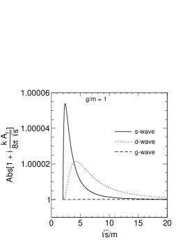
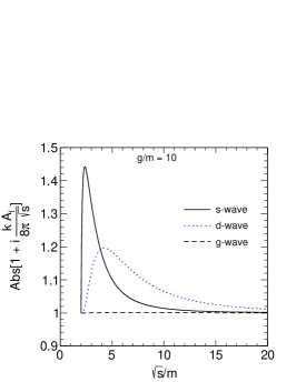
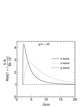
Figure 1: Energy dependence of the absolute value of $1+i\frac{kA_{l}}{8\pi\sqrt{s}}$ for $l=0,2,4$ at $g=1m$ (Left), $g=10m$ (Middle) and $20m$ (Right) at the tree-level.

II.2 Unitarization

In this subsection, we describe the so-called on-shell unitarization Dobado:1992ha ; Oller:1997ng . First, we need to introduce the $\varphi\varphi$ loop $\Sigma(s)$. Its imaginary part above the threshold is the usual phase-space kinematic factor (see e.g. Ref. Giacosa:2007bn ):

$$I(s)=\operatorname{Im}\Sigma(s)=\frac{1}{2}\frac{\sqrt{\frac{s}{4}-m^{2}}}{8\pi\sqrt{s}}\text{ for }\sqrt{s}>2m\text{ .}$$ (23)

We use no cutoff, hence the above equation is considered valid up to arbitrary values of the variable $s$. The imaginary part alone does not fix the form of $\Sigma(s)$ completely. Here, the loop function $\Sigma(s)$ for a complex $s$ is chosen by considering two subtractions Giacosa:2021brl :

$$\Sigma(s)=-\dfrac{(s-m^{2})(s-3m^{2})}{\pi}\int_{4m^{2}}^{\infty}\frac{\frac{1}{2}\frac{\sqrt{\frac{s^{\prime}}{4}-m^{2}}}{8\pi\sqrt{s^{\prime}}}}{(s-s^{\prime}+i\varepsilon)(s^{\prime}-m^{2})(s^{\prime}-3m^{2})}ds^{\prime}\text{ .}$$ (24)

The subtractions guarantee that $\Sigma(s=m^{2})=0$ and $\Sigma(s=3m^{2})=0.$ In this way, the choice of $\Sigma(s)$ fulfills the following requirements: (i) it preserves the pole corresponding to $s=m^{2}$ (in other words, the tree-level mass is also preserved at the unitarized level); (ii) it assures that the unitarized amplitude diverges at the branch point $s=3m^{2}$ generated by the single-particle pole for $m^{2}$ along the $t$ and $u$ channels.

Note, that the convergence of the integral is guaranteed by a single subtraction. Yet, it turns out that in the present approach a single subtraction is not appropriate to study our system, since, whenever a bound state forms, also a ghost state appears Donoghue:2019fcb . This problem does not take place when two subtractions as in Eq. 24 are implemented. A single subtraction is possible if a different unitarization loop is implemented, see Appendix B for details. Interestingly, the same unitarization procedure has been used in the recent work of Ref. Giacosa:2021brl dealing with glueball-glueball scattering in an effective dilaton model of Yang-Mills theory.

The real and the imaginary parts of $\Sigma$ as a function of $\sqrt{s}/m$ are shown in Fig. 2. [Note: throughout this paper, we consider $m=1$ in arbitrary unit (a.u.) and all the variables are normalized w.r.t. $m$.] The function $\operatorname{Re}\Sigma(s)$ vanishes at $\sqrt{s}/m=1$ and $\sqrt{3}$ as a consequence of the subtractions. In particular, it is positive between $\sqrt{s}/m=\sqrt{3}$ and the threshold $\sqrt{s}/m=2$, where it reaches the value

$$\Sigma(s=4m^{2})=\frac{3\pi+i\ln\left(\frac{1728(3-i\sqrt{3})^{3}}{(-36-12i\sqrt{3})^{3}}\right)}{64\sqrt{3}\pi^{2}}=\frac{1}{64\sqrt{3}\pi}\approx 0.0028715\text{ .}$$ (25)

In this way a bound state, if existent, has a mass within $(\sqrt{3}m,2m)$. Above threshold, $\operatorname{Re}\Sigma(s)$ decreases and becomes negative at large $\sqrt{s}/m$. Conversely, the imaginary part $\operatorname{Im}\Sigma(s)$ is zero (or better infinitesimally small) below the threshold, while above the threshold it increases according to Eq. (23). It is also useful to re-express the imaginary part $\operatorname{Im}\Sigma(s)$ as:

$$\operatorname{Im}\Sigma(s)=\left\{\begin{array}[c]{c}\frac{1}{2}\frac{\sqrt{\frac{s}{4}-m^{2}}}{8\pi\sqrt{s}}+\epsilon\text{ for }s>\left(2m\right)^{2}\\ \epsilon\text{ for }s<\left(2m\right)^{2}\end{array}\right.\text{ ,}$$ (26)

where $\epsilon$ is an infinitesimal positive quantity, see Appendix B for proper treatment of this issue. As discussed later on, this formal point is relevant when extending the phase shift below the threshold upon considering a small but finite $\varepsilon$.

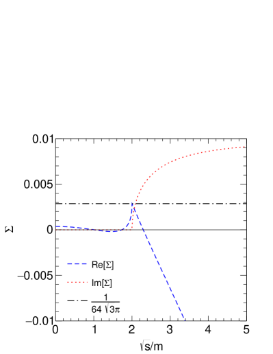
Figure 2: Energy dependence of the real and imaginary parts of the loop function $\Sigma$ (see Eq. 24). The value of the $\Sigma$ at the threshold ($=1/(64\sqrt{3}\pi)$) is also indicated in this plot.

The unitarized amplitudes are obtained by a resummation of the tree-level amplitudes $A_{k}(s)$ by assuming that the loop function of Eq. (24) can be factorized out:

$$A_{k}^{U}(s)=A_{k}(s)+A_{k}(s)\Sigma(s)A_{k}(s)+...=A_{k}(s)+A_{k}(s)\Sigma(s)A_{k}^{U}(s)\text{ ,}$$ (27)

thus a Bethe-Salpeter-type equation (e.g. Ref. Nieves:1998hp ) is obtained. Hence, the final expression reads:

$$A_{k}^{U}(s)=\left[A_{k}^{-1}(s)-\Sigma(s)\right]^{-1}\text{ .}$$ (28)

It is interesting to notice that, if we would keep only the $s$ channel for the case $l=0$, the tree-level amplitude reduces to $A_{l=0}(s)\simeq\frac{-g^{2}}{s-m^{2}},$ then the corresponding unitarized version is $A_{l=0}^{\text{U}}(s)\simeq\frac{-g^{2}}{s-m^{2}+g^{2}\Sigma(s)}$ with $\Sigma(s)$ is the loop function given in Eq. (24). Thus, the resummed propagator in the $s$-channel emerges. Yet, this is not a good approximation here, since the $t$ and $u$ channels are relevant, especially close to the threshold and for the eventual emergence of a bound state. The situation is different when two scalar fields are considered, in which one of them represents a resonance: in that case, the $s$-channel might be a good approximation, see Sec. IV.

Once the unitarized amplitudes are determined, the unitarized phase shift is calculated as:

$$\frac{e^{2i\delta_{l}^{U}(s)}-1}{2i}=\frac{1}{2}\cdot\frac{k}{8\pi\sqrt{s}}A_{l}^{U}(s)\text{ ,}$$ (29)

hence:

$$\delta_{l}^{U}(s)=\frac{1}{2}\arg\left[1+i\frac{k}{8\pi\sqrt{s}}A_{l}^{U}(s)\right].$$ (30)

Note, one can calculate $\delta_{l}^{U}(s)$ by using the equivalent expressions

$$\delta_{l}^{U}(s) =\frac{1}{2}\arcsin\left[\frac{k}{8\pi\sqrt{s}}\operatorname{Re}\left[A_{l}^{U}(s)\right]\right]=\frac{1}{2}\arccos\left[1-\frac{k}{8\pi\sqrt{s}}\operatorname{Im}\left[A_{l}^{U}(s)\right]\right]\text{ .}$$ (31)

In fact, when unitarization is preserved, the expressions in Eq. (31) and (30) give rise to the same result for the phase shift. This is also a practical useful check of the validity of unitarity. The unitarization of amplitudes that contains a sizable contribution of $t$ and $u$ channel exchanges is discussed in various works, especially in the domain of pion-pion (or other hadronic) scattering phenomena Black:2000qq ; Dobado:1992ha ; Delgado:2015kxa ; Oller:1997ng ; Guo:2006br ; Gulmez:2016scm ; Oller:2020guq ; Giacosa:2021brl . In practice, any unitarization simplifies in some form the underlying Lippmann-Schwinger equations. The on-shell approximation used here means that the $t$ and the $u$ channels are evaluated on-shell, implying that our results for the formation of a bound state are acceptable when the coupling constant $g$ is not too large, see next Section. Namely, this unitarization does not describe properly the left-hand cut that starts at $s=3m^{2}$.

The unitarized scattering length reads:

$$a_{0}^{U,\text{SL}}=\frac{1}{2}\frac{1}{16\pi m}\frac{1}{A_{0}^{-1}(4m^{2})-\Sigma(4m^{2})}=\frac{1}{32\pi m}\frac{1}{\frac{3m^{2}}{5g^{2}}-\frac{1}{64\sqrt{3}\pi}\text{.}}\text{.}$$ (32)

The critical value of $g$ is given by:

$$\frac{3m^{2}}{5g^{2}}-\frac{1}{64\sqrt{3}\pi}=0\rightarrow\frac{g_{c}^{2}}{m^{2}}=\frac{192\sqrt{3}\pi}{5}\approx 208.95\text{ ,}$$ (33)

thus

$$\frac{g_{c}}{m}\approx 14.4551\text{ .}$$ (34)

For $g=g_{c}$ the divergence of the scattering length signalizes the emergence of a bound state just at the threshold, see next subsection.

When $g$ approaches $g_{c}$ the tree-level scattering length becomes less and less accurate. While for $g/m=1$ the ratio of the tree-level and the unitarized scattering length is $a_{0}^{\text{T,SL}}/a_{0}^{\text{U,SL}}=0.995,$ already for $g/m=5$ one gets $a_{0}^{\text{T,SL}}/a_{0}^{\text{U,SL}}=0.88.$ By further increasing the coupling to $g/m=10$ implies $a_{0}^{\text{T,SL}}/a_{0}^{\text{U,SL}}=0.52,$ which corresponds to a sizable underestimation w.r.t. the unitarized result. For values exceeding $g_{c}$ the tree-level results are not meaningful any longer, since no bound state forms. These numbers, together with the previously presented Fig. 1, show that a unitarization is required if $g/m$ of the order of 10-20 needs to be investigated.

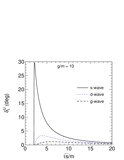
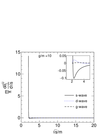
Figure 3: (Left) Energy dependence of the phase shifts (using Eqs. 28 and 30) for $l=0,2,4$ at $g=10m<g_{c}$. (Right) Energy dependence of derivatives of the phase shifts.

Before going into the details of the numerical results of the phase shifts, let us mention the convention adopted in this work. We impose that the phase shifts for any partial waves vanish at the threshold:

$$\delta_{l}^{U}(s=4m^{2})=0\text{ .}$$ (35)

Sometimes a different convention is used, according to which the phase space at the threshold equals $n_{B}\pi$, where $n_{B}$ is the number of bound states below the threshold Taylor . Since the physical quantities are related to the difference and derivative of the phase shifts, the results are unaffected by the choice of the convention of the phase shift at the threshold.

The left panel of Fig. 3 shows the energy dependence of the unitarized phase shifts for s-wave ($l=0$), d-wave ($l=2$), and g-wave ($l=4$) at the coupling $g=10m<g_{c}\approx 14.45m$. The s-wave phase shift increases rapidly just above the threshold $\sqrt{s}=2m$ and then decreases approaching zero at large energies. The d-wave and g-wave show similar behavior, yet their magnitudes are smaller than that of the s-wave. (Note, the degeneracy factor ($2l+1$) is not displayed in Fig. 2). The corresponding phase shift derivatives are depicted in the right panel of Fig. 3 .

Figure 4 shows the same quantities as Fig. 3 but for $g=20m>g_{c}$. The s-wave phase shift, shown in the left panel, decreases rapidly above the threshold and saturates at $-\pi$ at large $\sqrt{s}/m$. This behavior indicates the presence of a bound state below the threshold, see the next subsection. The phase shifts of d- and g-waves are similar to the previous case. The right panel shows the derivatives of the phase shifts, where it is visible that the s-wave contribution is sizable.

The phase shift in Eq. (29) is defined only for $s\geq 4m^{2}.$ Yet, following the discussion of Ref. Samanta:2020pez , upon using Eq. (26) one can extend the phase shift also below the threshold by considering the expression upon considering an arbitrarily small but nonzero $\varepsilon$:

$$\delta_{l}^{U}=\frac{1}{2}\arg\left[1+2iA_{l}^{U}\operatorname{Im}\Sigma\right]\text{ }.$$ (36)

Above the threshold, we recover Eq. 30. Below the threshold, the equation $\operatorname{Im}\Sigma=\epsilon$ implies that $\delta_{l}^{U}=n\pi=const$ for any finite $A_{l}^{U}$ (the choice $n=0$ guarantees that the phase shift is continuous at the threshold). Yet, the situation is different if pole(s) of $A_{l}^{U}$ appear(s) (indeed, the single-particle pole below the threshold for $s=m^{2}$ is always present in the $\varphi^{3}$-theory), see the next Section.

Here, we briefly discuss the intuitive meaning of the extension above. The $\varepsilon$ prescription makes the particle $\varphi$ ‘slightly unstable’, because the pole is realized for $s=m^{2}-i\varepsilon/2$, see Appendix B. Since the particle $\varphi$ is unstable and its width is proportional to $\varepsilon$, its mass distribution is not exactly a Dirac delta (it becomes such for $\varepsilon\rightarrow 0$). Then, the scattering below the threshold $2m$ is possible (even though very small and vanishing for $\varepsilon\rightarrow 0$ as expected). The bound state, if existent, is itself slightly unstable, the width is also proportional to $\epsilon\propto\varepsilon$ (see the next subsection), and thus can be seen as a resonance produced in a scattering process. In this way, as discussed in Sec. III.A an alternative view is possible to understand the inclusion of the bound state and one may show that the pressure as a function of the coupling is continued when the latter forms. Yet, the result is not dependent on $\varepsilon$ in the limit $\varepsilon\rightarrow 0$.

We conclude this subsection with some general considerations. As discussed above, Eq. (26) does not fix the real part of the loop. The two subtractions used for the determination of the loop function $\Sigma(s)$ of Eq. (24) guarantee convergence and the absence of unphysical states, but any number of subtractions would be consistent with Eq. (26), even though it would be hard to physically justify a choice with many subtractions. Alternatively, one may also include a form factor by modifying the imaginary part itself, $\operatorname{Im}\Sigma(s)=\frac{1}{2}\frac{k}{8\pi\sqrt{s}}e^{-k^{2}/\Lambda^{2}}$ with $k=\sqrt{\frac{s}{4}-m^{2}}.$ Such form factors are sometimes used in hadronic theories (e.g. Amsler:1995td ; Faessler:2003yf ; Giacosa:2007bn ) since they model the finite extension of hadrons. In this case, the real part is finite even without applying a subtraction (for technical details, see e.g. Ref. Coito:2019cts ).

Indeed, various unitarization approaches have been explored in the literature, e.g. Refs. Oller:2020guq ; Mai:2022eur ; some of them go beyond the on-shell approximation used here. One interesting unitarization scheme that was widely used in the past is the so-called $N/D$ approach Frazer:1969euo ; Hayashi:1967bjx ; Gulmez:2016scm ; Oller:2020guq ; Cahn:1983vi ; Mai:2022eur ; Giacosa:2021brl , where $N$ stays for the numerator and $D$ for the denominator. The basic idea is that the unitarized amplitude can be written as a ratio of functions, where the numerator contains the left-hand cut and the denominator the right-hand cut. In Appendix B we present this unitarization scheme (for simplicity, at its lowest order) for the $\varphi^{3}$-case. In this way, we can compare the results of this alternative unitarization scheme (phase shifts, the critical value of the coupling for the emergence of a bound state and the mass of the latter as a function of $g$, as well as the behavior of the pressure) with the results presented in the main text. As the outcomes show, the overall qualitative picture is left unchanged, which makes us confident that the features that we present are not just inherent to the employed unitarization approach.

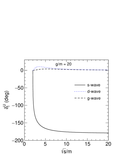
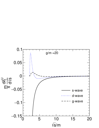
Figure 4: Energy dependence of the phase shifts (using Eqs. 28 and 30) for $l=0,2,4$ at $g=20m>g_{c}$. (Right) Energy dependence of the derivatives of the phase shifts.

II.3 Bound state

Figure 5: Dependence of the bound state mass (Eq. 37) with the coupling $g$. The vertical line indicates the critical coupling $g_{c}$, for which $M_{B}=2m$.

We describe here the emergence of the bound state that takes place when the attraction is sufficiently strong. The bound state equation ($s$-channel, for the Mandelstam variable $s$ continued below the threshold) corresponds to a pole of the amplitude in Eq. 28:

$$\left[A_{0}^{-1}(s)-\Sigma(s)\right]=0\text{ .}$$ (37)

In Fig. 5 the mass of the bound state $M_{B}/m$ is plotted as a function of the coupling $g$. For the critical value $g=g_{c}+\epsilon\approx 14.45m$ the bound state forms exactly at threshold, and for $g>g_{c}$ it ranges between $\sqrt{3}<\sqrt{s}/m<2$, in which $\operatorname{Re}\Sigma(s)>0$. Note that when a bound state is close to threshold forms, it can be also understood via non-relativistic approaches, see e.g. Ref. Baru:2003qq ; Hayashi:1967bjx ; Dong:2008mt .

In particular, the limit $M_{B}(g\rightarrow\infty)=\sqrt{3}m$ holds. Thus, the results are finite also for arbitrarily large values of $g$. However, this property is a consequence of the employed unitarization but is not physical. Namely, one could choose other unitarization approaches that deliver different results for the limit $g\rightarrow\infty$. In the already mentioned $N/D$ method (see Appendix B), the bound state forms for a similar critical value of the coupling constant ($g_{c}=13.02m$) and the behavior of the bound state as a function of $g$ well compares to Fig. 5 for $g$ up to (and even slightly above) $20m$, but then the results deviate from each other. In particular, in the $N/D$ approach $M_{B}(g\rightarrow\infty)=m$. This is also an artifact of that particular method with the constraints described in Appendix B.

In general, different unitarization approaches usually come up with similar values for the critical coupling for which the bound state emerges, but depart from each other when the attraction is too strong. Actually, for $g$ very large one should encounter a solution of the type $M_{B}^{2}<0$ that signalizes an instability, as the potential of Eq. 2 suggests, but this feature is not described by the twice-subtracted on-shell unitarization approach used in this work.

Summarizing our discussion, the plateau $M_{B}(g\rightarrow\infty)=\sqrt{3}m$, see also Fig. 5, is an artifact of our unitarization. For this reason, we consider a value of $g/m$ of about $40$ (before the plateau sets in) as an upper limit of our approach (in our numerical examples, we shall actually limit our studies to $g/m\lesssim 20$). Thus, the introduction of unitarization allows us to go further than what the tree-level results do, yet not to arbitrarily large coupling constants. More advanced unitarization approaches could extend the range of $g$, but this is left for the future.

In Fig. 6 we present the s-wave phase shift and its derivative by using the extended version of Eq. (40) that contains also the continuation below the threshold. This is indeed an important extension since it allows to accommodate the bound state in the phase-shift formula. In order to discuss these aspects, we recall that for $s<4m^{2}$:

$$A_{l}^{U}\operatorname{Im}\Sigma=\frac{\epsilon}{A_{0}^{-1}-\Sigma}=\frac{\epsilon}{A_{0}^{-1}-\operatorname{Re}\Sigma-i\operatorname{Im}\Sigma}=\frac{\epsilon}{A_{0}^{-1}-\operatorname{Re}\Sigma-i\epsilon}\text{ .}$$ (38)

For $g<g_{c}$ no bound state occurs, thus $\delta_{l}^{U}(x=\sqrt{s})=0$ for $\sqrt{3}m\leq x\leq 2m.$ For $g>g_{c}$ a bound state occurs for a certain $s=M_{B}^{2}$ belonging to the interval $(3m^{2},4m^{2})$, thus

$$\left(A_{l}^{U}\operatorname{Im}\Sigma\right)_{s=M_{B}^{2}}=\frac{\epsilon}{-i\epsilon}=i\text{ ,}$$ (39)

which in turn shows why it is important to keep track of the $i\epsilon$ factors in the energy region below the threshold. It then follows that $\delta_{l}^{U}(x=M_{B})=n\frac{\pi}{2}.$ Upon requiring (for $\epsilon$ small but finite) a continuous phase shift, $\delta_{l}^{U}(x)$ for $\epsilon\rightarrow 0$ reads

$$\delta_{l}^{U}(x=\sqrt{s})=-\pi+\pi\theta(x-M_{B})\text{ for }\sqrt{3}m\leq x\leq 2m\text{ and }g>g_{c}\text{ ,}$$ (40)

whose derivative is a Dirac delta: $\pi\delta(x-M_{B}).$ In a certain sense, this result is quite intuitive: even though the physical range is realized for $s\geq 4m^{2},$ when the continuation to the region below the threshold is performed the bound state corresponds to a very narrow object (width proportional to $\epsilon$) that is encountered along the $s$-axis and implies an increase of the phase shift of $\pi$ (see also Sec. 4 for the conceptually analogous case of a resonance).

Moreover, the amplitude $A_{l}^{U}$ has a second pole for $s=m^{2}$ (the single-particle pole that is also exchanged in the $s$-channel). Then, also for this value Eq. 39 applies. The phase shift can be further extended below the threshold as:

$$\delta_{l}^{U}(x=\sqrt{s})=-2\pi+\pi\theta(x-m)+\pi\theta(x-M_{B})\text{ for }0\leq x\leq 2m\ \text{ and }g>g_{c}\text{ ,}$$ (41)

whose derivative is $\pi\delta(x-m)+\pi\delta(x-M_{B})$, hence including both the particle $\varphi$ and the bound state $B.$

Figure 6: (Left) Energy dependence of the s-wave phase shift at $g=20m>g_{c}$ below and above the threshold. One may note the jump from $-\pi/2$ at the bound state mass $M_{B}$. (Right) Corresponding energy dependence of the derivative of the phase shift. At $\sqrt{s}=M_{B}$ a Dirac-delta function appears.

In the end, we have verified that the phase shifts studied above fulfill the so-called causality Wigner condition in the form discussed in Ref. Boglione:2002vv :

$$\frac{d\delta_{l}}{dx}\geq-\frac{x^{2}}{8\left(\frac{x^{2}}{4}-m^{2}\right)}\text{ ,}$$ (42)

see Appendix C for more details and related plots.

III Thermodynamic properties of the $\varphi^{3}$-QFT

In this section, we study the $\varphi^{3}$-theory at nonzero temperature. In particular, we shall concentrate on the evaluation of the different contributions to the pressure. To this end, we use the phase shift (or S-matrix) formalism Dashen:1969ep ; Venugopalan:1992hy ; Broniowski:2015oha ; Lo:2017ldt ; Lo:2017sde ; Lo:2017lym ; Dash:2018can ; Dash:2018mep ; Lo:2019who ; Lo:2020phg (for a brief recall see Appendix A), which allows calculating the pressure (or any other thermodynamic quantity) from the vacuum’s phase shifts. Intuitively, the idea behind this approach is that the energy levels $E_{n}$ entering into the partition function $Z=\sum_{n}e^{-E_{n}/T}$ are determined in the vacuum. Basically, the derivatives of phase shifts are proportional to the density of states that enter in $Z$.

In this respect, this approach is different from thermal field theory Kapusta:2006pm (see for instance works involving the CJT formalism as well as other thermal approaches in Refs. Rischke:2003mt ; Brambilla:2014jmp ; Lenaghan:1999si ; Papazoglou:1996hf ; Amelino-Camelia:1996sfy ; Tolos:2008di ; GomezNicola:2002tn ; Carrington:1999bw and refs. therein), since one needs only vacuum results to obtain thermodynamic quantities. The knowledge of the latter is relatively simple if one considers only elastic two-body scattering, but becomes more and more complicated when inelastic processes and multiple channels become relevant Lo:2020phg . Thus, the S-matrix approach is expected to be valid for (relatively) low temperatures.

In practice, we shall evaluate the (various contributions to the) pressure of the system as a function of $g$ for fixed $T$ and as a function of $T$ for selected $g$. Then, we shall discuss deviations from the simple free gas results.

III.1 Nonzero-$T$ formalism

The non-interacting part of the pressure for gas of interacting particles with mass $m$ reads:

$$P_{\varphi\text{,free}}=-T\int_{k}\ln\left[1-e^{-\beta\sqrt{k^{2}+m^{2}}}\right]\text{ ,}$$ (43)

where $\int_{k}\equiv\int d^{3}k/(2\pi)^{3}$ and $\beta=1/T$. Let us then include interaction and, at first, assume that no bound state forms. In the scattering-matrix or the $S$-matrix formalism Dashen:1969ep ; Venugopalan:1992hy ; Broniowski:2015oha ; Lo:2017ldt ; Lo:2017sde ; Lo:2017lym ; Dash:2018can ; Dash:2018mep ; Lo:2019who , the interacting part of the pressure is related to the derivative of the phase shift with respect to the energy by the following relation:

$$P_{\varphi\varphi\text{-int}}^{U}=-T\int_{2m}^{\infty}dx\frac{2l+1}{\pi}\sum_{l=0}^{\infty}\frac{d\delta_{l}^{U}(s=x^{2})}{dx}\int_{k}\ln\left[1-e^{-\beta\sqrt{k^{2}+x^{2}}}\right]=\sum_{l=0}^{\infty}P_{\varphi\varphi\text{-int},l}^{U}\text{ ,}$$ (44)

where $x=\sqrt{s}$. In the previous equation, the usual thermal integral’s contribution for gas of particles with running mass $x$ is weighted by the vacuum’s phase shift derivatives, see Appendix A. Eq. 44 shows that the contribution to the pressure of a certain wave is positive if $\frac{d\delta_{l}}{dx}>0$ and negative if $\frac{d\delta_{l}}{dx}<0.$ For $x$ close to the threshold, these two cases correspond to attraction and repulsion, respectively (but this is not true in general). If, for instance, $\delta_{l}$ increases from the threshold up to a certain maximum and then decreases to zero for large $x,$ the overall contribution is expected to be positive, since low values of $\sqrt{s}=x$ are the dominant ones in the thermal integrals.

It may be at first sight puzzling that an attraction generates an increase of pressure, since one is rather used to thinking in terms of a classic Van-der-Walls gas of particles in which (for a fixed number of particles) an attraction implies a smaller pressure (and vice-versa, a repulsion means a larger pressure). Yet, our case here is different: an attraction implies that the density of states increases (roughly speaking, more states are present), thus the pressure becomes larger (the opposite applies to a repulsion).

Summarizing, the total pressure reads

$$P_{\text{tot}}^{U}=P_{\varphi\text{,free}}+P_{\varphi\varphi\text{-int}}^{U}\text{ .}$$ (45)

Above, it should be noted that the free part is calculated at the physical mass $m$ which, due to suitable resummations, is left unchanged by loop corrections. In this way, in the interacting case, $P_{\varphi\text{,free}}$ may be interpreted as the pressure of the asymptotic states of the system.

Next, let us move to the case in which a bound state exists, that is the coupling $g$ is larger than the critical value $g=g_{c}$. The following considerations are in order:

• The pressure of Eq. (45) has a jump as a function of $g$ at $g_{c}$ at $a$ given temperature $T$. This is due to the different behavior of the s-wave phase-shift if the bound state is present: the corresponding contribution changes sign. This abrupt jump in the pressure signalizes that ‘something is missing’ in Eq. (45). It is rather natural to think that the missing element is indeed the emerging bound state.

• The first approach is to consider that a bound state is an additional asymptotic state of the system. In this way, the bound state with mass $M_{B}$ is expected to correspond to an additional state that needs to be added to the expression of Eq. (44), thus:

  $$P_{B}\overset{\text{ }}{=}-\theta(g_{c}-g)T\int_{k}\ln\left[1-e^{-\beta\sqrt{k^{2}+M_{B}^{2}}}\right]\text{ ,}$$ (46)

  where the theta function takes into account that for $g<g_{c}$ there is no bound state $B.$ Indeed, this simple and intuitive expression turns out to be consistent with the regulating procedure adopted in this work, see below. The total pressure of the system is written as

  $$P_{\text{tot}}^{U}=P_{\varphi\text{,free}}+P_{B}+P_{\varphi\varphi\text{-int}}^{U}\text{ .}$$ (47)

  On top of the $\varphi\varphi$ interactions, there are also $B\varphi$ and $BB$ interactions, which however can be neglected in the energy and temperatures of interest.

• Another way to justify and obtain the result above goes via the $\varepsilon$-driven extension of the phase-shift formula below the threshold presented in Sec. II.C (see also Appendix B and Ref. Samanta:2020pez ). Namely, the bound state (if it forms) can be seen a manifestation of the interaction among the $\varphi$ particles and is interpreted as a very narrow resonance below the threshold. Thus, upon extending the interaction range in Eq. (44), the whole interaction contribution (including the bound state if existent) reads:

  $$P_{\varphi\varphi\text{-int}}^{U}+P_{B}=-T\int_{\sqrt{3}m}^{\infty}dx\frac{2l+1}{\pi}\sum_{l=0}^{\infty}\frac{d\delta_{l}^{U}(s=x^{2})}{dx}\int_{k}\ln\left[1-e^{-\beta\sqrt{k^{2}+x^{2}}}\right]\text{ ,}$$ (48)

  where the lowest range of the integral is set to $\sqrt{3}m$, since the bound state mass belongs to the interval $(\sqrt{3}m,2m)$. The bound state contribution (if the bound state forms) corresponds to the integral range between $(\sqrt{3}m,2m)$:

  $$P_{B}=-T\int_{\sqrt{3}m}^{2m}dx\frac{2l+1}{\pi}\sum_{l=0}^{\infty}\frac{d\delta_{l}^{U}(s=x^{2})}{dx}\int_{k}\ln\left[1-e^{-\beta\sqrt{k^{2}+x^{2}}}\right]$$

  $$=-\theta(g_{c}-g)T\int_{k}\ln\left[1-e^{-\beta\sqrt{k^{2}+M_{B}^{2}}}\right]\text{ ,}$$ (49)

  where the r.h.s. is obtained by using Eq. (40). The properties discussed above are actually applicable to any QFT that displays bound states: if present, they appear as infinitely narrow states that can be (formally) created by particle scattering extended below the threshold.

• The two interpretations above (including the bound state as an additional asymptotic state or as part of the interaction as a narrow resonance) lead to the same result of Eq. (47). Yet, in the latter case, one still has the same set of asymptotic states that coincide with the states of the theory realized for $g=0$, because the bound state is seen as part of the interaction. (A subtle difference between the $g>0$ and the $g=0$ case is present in the model described in Sec. IV).

• As anticipated in the introduction and shown later on in various examples, the expression in Eq. (48) is continuous as a function of $g$ for any fixed value of $T$. This is an additional confirmation of the consistency of the proposed expression, since a non-analytic point of the pressure as a function of the coupling constant would not be a physical feature. The jump due to the emergence of the bound state is compensated by a jump in the contribution to the pressure arising from the particle interaction above the threshold. Indeed, upon considering a small quantity $\alpha$, one has that

  $$\frac{1}{\pi}\left[\left(\frac{d\delta_{0}^{U}(x)}{dx}\right)_{g=g_{c}-\alpha}-\left(\frac{d\delta_{0}^{U}(x)}{dx}\right)_{g=g_{c}+\alpha}\right]\simeq\delta(x-2m)\text{ ,}$$ (50)

  thus the jump of the interaction pressure due to the change in the phase space behavior matches a state just a t threshold:

  $$\left(P_{\varphi\varphi\text{-int}}^{U}\right)_{g=g_{c}-\alpha}-\left(P_{\varphi\varphi\text{-int}}^{U}\right)_{g=g_{c}+\alpha}=\left(P_{B}\right)_{M_{B}=2m}\text{ ,}$$ (51)

  thus showing that the pressure is continuous as a function of $g$.

• Interestingly, in the particular case of the $\varphi^{3}$-theory, one may go even further and describe the total pressure via the phase shift formula as

  $$P_{\text{tot}}^{U}=-T\int_{0}^{\infty}dx\frac{2l+1}{\pi}\sum_{l=0}^{\infty}\frac{d\delta_{l}^{U}(s=x^{2})}{dx}\int_{k}\ln\left[1-e^{-\beta\sqrt{k^{2}+x^{2}}}\right]\text{ ,}$$ (52)

  in which the lowest range of the integral is set to zero. This is not possible in general but holds here because of the nature of the $\varphi^{3}$ self-interaction: the very same particle $\varphi$ is also exchanged in the $s$-channel of $\varphi\varphi$ scattering.

In the end, we stress that above we have presented a series of plausible arguments to properly include a bound state in the phase-shift formalism. Surely a formally more rigorous approach would be needed in the future to fully clarify the procedure and the issues raised here.

III.2 Numerical results

Next, we turn to numerical examples and plots that allow showing the properties of the system at nonzero temperature.

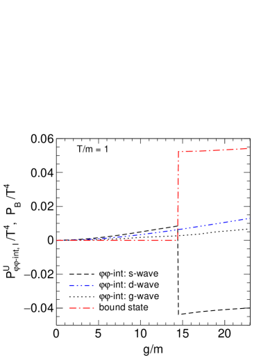
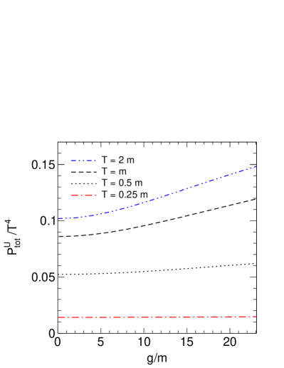
Figure 7: Left panel shows $P^{U}_{\varphi\varphi\text{-int},l}/T^{4}$ of Eq. 44) as function of $g/m$ for three different partial waves corresponding to $l=0$ (s-wave), $l=2$ (d-wave) and $l=4$ (g-wave) at $T/m=1$. The bound state contribution ($P_{B}/T^{4}$) (Eq. 46) is also shown. The right panel shows the normalized total pressure (Eq. 47) at four different temperatures.

The unitarized pressure ($P^{U}_{\varphi\varphi\text{-int},l}/T^{4}$) is shown in Fig. 7 as a function of $g/m$ at $T/m=1$ for the partial waves corresponding to $l=0,2,4$. The s-wave is interesting: up to $g=g_{c}\approx 14.45m$, increases, then it abruptly jumps to negative values. The reason is that above $g_{c}$ a bound state exists. The normalized pressure ($P_{B}/T^{4}$) for the bound state (see Eq. 46) is also shown: it is zero below $g_{c}$ and nonzero (and positive) above this value. The jump has the same magnitude but the opposite sign of the s-wave interacting channel. Moreover, the normalized total pressure $P_{tot}^{U}/T^{4}$ with $g/m$ as evaluated via Eq. 47, shown in the right panel of Fig. 7, varies continuously with $g$ in all four temperatures shown in this figure. This fact confirms one of the main outcomes of the paper: when interactions are taken into account, the formation of a new state does not correspond to any sudden jump in the pressure or energy density of the system.

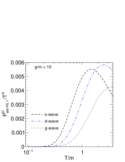
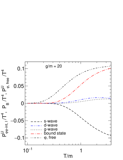
Figure 8: The left panel shows the temperature dependence of the interacting normalized pressure (see Eq. 44) for s-, d- and g-waves at $g=10m<g_{c}$. Right panel shows a similar plot but for $g=20m>g_{c}$ when bound state is produced. Besides the interactions of s-, d- and g-waves, the normalized pressure of the bound state and of free particles are also shown.

Next, Fig. 8 shows the interacting parts of the normalized pressure ($P^{U}_{\varphi\varphi\text{-int},l}/T^{4}$) for the s-, d- and g-waves as a function of $T/m$ for $g=10m<g_{c}$ (no bound state). This figure offers also an additional indication of the range of temperatures for which we may trust our results. For $T/m\sim 1$ the s-wave dominates and the higher waves represent a small correction. For $T/m\sim 2$, the d-wave contribution becomes as large as the s-wave one, thus caution is required. Yet, the g-wave contribution is still safely small and we may argue that the further contributions are still negligible. In addition, we recall that at $T/m\sim 3$ inelastic channels become relevant. We thus consider $T/m\sim 3$ as an upper limit of our study. For these reasons, in this figure (as well as in all other figures presenting the pressure contributions as a function of $T/m$) we use a logarithmic plot in order to underline the low-T part of our results up to $T/m\sim 3$. Whenever a fixed $T/m$ value is required, the maximal one used in this work is $T/m=2$, see e.g. Fig.7.

The total normalized pressure as a function of $T/m$ is shown in Fig. 9 for three different values of $g$ (the free case $g=0$, $g/m=10$ and $g/m=20$). At high $T$ the massless limit $(P_{\varphi,\text{free}}/T^{4})_{m=0}=\pi^{2}/90\approx 0.1096$ is reached.

For completeness, we have studied the speed of sound

$$c_{s}^{2}=\frac{\partial P}{\partial\varepsilon}=\frac{P^{\prime}(T)}{\varepsilon^{\prime}(T)}=\frac{P^{\prime}(T)}{TP^{\prime\prime}(T)}$$ (53)

which is safely smaller than one for all investigated temperatures, see Appendix C for details (in the r.h.s. above, the thermodynamical self-consistency $\varepsilon=TP^{\prime}-P$ has been used.)

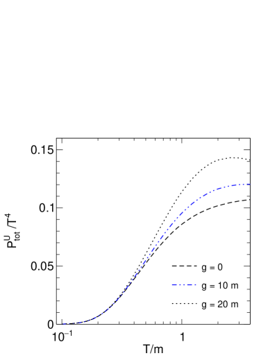
Figure 9: Temperature dependence of the normalized total pressure (Eq. 47).

An important point concerns the quantification of the contribution of the interaction to the pressure. We discuss the scenarios without and with the bound state separately. When no bound state forms ($g<g_{c}$), it is useful to define the quantity:

$$\eta=\frac{P^{U}_{\text{tot}}}{P_{\varphi\text{,free}}}=1+\frac{P^{U}_{\varphi\varphi-\text{int}}}{P_{\varphi\text{,free}}}\text{ .}$$ (54)

The absence of interactions ($g\rightarrow 0$) corresponds to $\eta=1$ and departures from this value quantify the naive result that one obtains by neglecting them.

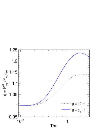
Figure 10: Temperature dependence of the ratio $\eta$ (Eq. 54) (Left) and $\zeta$ (Eq. 55) (Right).

The left panel of Fig. 10 shows the temperature dependence of $\eta$ for two different values of $g<g_{c}$. For both cases $\eta\approx 1$ when $T$ is low. This indicates that the role of the interaction is negligible at low temperatures. With the increase of $T/m$, $\eta$ increases and becomes maximal at around $T/m\approx 2$. Moreover, we notice that for $g=g_{c}-\epsilon$ the maximum is reached for $\eta\approx 1.23$, which indicates that the effect of interaction is non-negligible at certain intermediate temperatures.

Let us now define an analogous quantity to be used when a bound state forms ($g>g_{c}$):

$$\zeta=\frac{P^{U}_{\varphi\varphi-\text{int}}+P_{B}}{P_{B}},$$ (55)

out of which the total pressure of the system is given by

$$P^{U}_{\text{tot}}=P_{\varphi\text{,free}}+\zeta P_{B}\text{ ,}$$ (56)

which is simply the sum of two free gases, one for the particles of the type $\varphi$ with mass $m$ and one for the bound state $B$ with mass $M_{B}$. Yet, the latter is rescaled by the factor $\zeta$, whose departure from unity quantifies how much of the bound state contribution remains after the partial cancellation induced by the interaction has been taken into account.

In the right panel of Fig. 10 we show the temperature dependence of $\zeta$ for the values $g=g_{c}+\varepsilon$ and $g=20m$. For $g=g_{c}+\varepsilon$, the quantity $\zeta\approx 0.4$ at $T/m=0.1$, which then decreases for increasing $T/m$ and saturates to $\approx 0.08$. For $g=20m$, $\zeta\approx 0.7$ at low $T/m$ and decreases to $\approx 0.08$ at high $T/m$. Thus, in both cases, the joint role of the bound state and interaction can be summarized by a contribution of free gas of bound state particles which is sizably reduced by $\zeta$. The amount of reduction depends both on the value of $g$ as the value of temperature, being typically larger at small $T$ and smaller at large $T$.

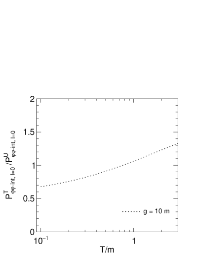
Figure 11: Dependence of the ratio of tree-level pressure and unitarized pressure for s-wave with $T/m$.

We conclude this section with two additional remarks:

• The introduced unitarization is a suitable tool for the study of bound states. It goes beyond perturbative results, which are not capable to generate poles below the threshold. Yet, even when no bound state forms but the coupling is not small, the role of unitarization is also non-negligible. This point has been already mentioned in Sec. II.B in connection with the scattering length. We show this feature also at nonzero $T$ in Fig. 11, where the ratio of the s-wave tree-level pressure and the unitarized one is plotted as a function of $T$ for $g/m=10.$ It is visible that the effect of the unitarization is in general non-negligible both at small and at large $T$.

• The potential in Eq. 1 is unbounded from below. A simple improvement is to add to the potential a term $\frac{\lambda}{4!}\varphi^{4}$ with $\lambda>0.$ This case is presented in Appendix D: in general, there are quantitative but not qualitative changes w.r.t. the results presented in this section, but also some additional problems related to this extension appear. The Wigner condition is not always fulfilled and the speed of sound exceeds 1 at high $T$, meaning that additional studies are required in the future.

IV An intermediate state $S$

In this section, we study the case in which two distinct particles, $\varphi$ with mass $m$ and $S$ with mass $M$, are considered. Their interaction is a three-leg $gS\varphi^{2}$ vertex. Thus, the decay of $S$ into $\varphi\varphi$, if kinematically allowed, takes place. Then, the state $S$ is a resonance with a certain decay width. Since two $\varphi$ particles interact via an exchange of $S$, an attractive Yukawa interaction between them is induced: if it is strong enough, a bound state forms. The main question here is how this system behaves at nonzero $T$.

IV.1 Vacuum’s formalism

The Lagrangian under study takes the form:

$$\mathcal{L}=\frac{1}{2}\left(\partial_{\mu}\varphi\right)^{2}-\frac{1}{2}m^{2}\varphi^{2}+\frac{1}{2}\left(\partial_{\mu}S\right)^{2}-\frac{1}{2}M^{2}S^{2}+\frac{g}{2!}S\varphi^{2},$$ (57)

where $g$ is the coupling constant. The tree-level decay width $S\rightarrow\varphi\varphi$ (allowed for $M>2m$) reads (e.g. Ref. Giacosa:2007bn ):

$$\Gamma_{S}=\frac{g^{2}}{2}\frac{\sqrt{\frac{M^{2}}{4}-m^{2}}}{8\pi M^{2}}\text{ ,}$$ (58)

and the tree-level scattering is:

$$A(s,t,u)=\frac{-g^{2}}{s-M^{2}+i\epsilon}+\frac{-g^{2}}{t-M^{2}+i\epsilon}+\frac{-g^{2}}{u-M^{2}+i\epsilon}\text{ .}$$ (59)

The first three tree-level partial wave amplitudes are evaluated as:

$$A_{0}(s)=\frac{1}{2}\int_{-1}^{+1}d\xi A(s,\theta)=-\frac{g^{2}}{s-M^{2}+i\epsilon}+2g^{2}\frac{\ln\left[1+\frac{s-4m^{2}}{M^{2}}\right]}{s-4m^{2}+i\epsilon}\text{ ;}$$ (60)

$$\begin{split}A_{2}(s)=&\frac{-2g^{2}}{(s-4m^{2})^{3}}(3\left(4m^{2}-s\right)(4m^{2}-2M^{2}-s)\\ &+\left(16m^{4}+6M^{4}+6M^{2}s+s^{2}-8m^{2}(3m^{2}+s)\right)\ln\left[1+\frac{s-4m^{2}}{M^{2}}\right])\text{ ;}\end{split}$$ (61)

$$\begin{split}A_{4}(s)=&\frac{-2g^{2}}{3(s-4m^{2})^{3}}[5(4m^{2}-s)(4m^{2}-2M^{2}-s)(80m^{4}-8m^{2}(21M^{2}+5s)+42M^{4}\\ &+42M^{2}s+5s^{2})-6(256m^{8}-256m^{6}(5M^{2}+s)+96m^{4}(15M^{4}+10M^{2}s+s^{2})\\ &-16m^{2}(35M^{6}+45M^{4}s+15M^{2}s^{2}+s^{3})+70M^{8}+140M^{6}s+90M^{4}s^{2}\\ &+20M^{2}s^{3}+s^{4})\ln(1+\frac{s-4m^{2}}{M^{2}})]\text{ .}\end{split}$$ (62)

Also, in this case, we limit our study to two-body $\varphi\varphi$ scattering processes. Within our framework, the state $S$ is a resonance, therefore it is not an asymptotic state of the theory. Namely, the scattering of the type $S\varphi\rightarrow S\varphi$ should be understood as part of the more general process $\varphi\varphi\varphi\rightarrow\varphi\varphi\varphi.$ They are omitted here since they are not expected to contribute much to the energies and temperatures of interest.

The unitarization is carried out by repeating analogous steps as in Sec. II.2. As previously, the loop function for $M<2m$ (when the state $S$ is stable) has therefore two subtractions, one at the mass $M$ and one at the branch point $4m^{2}-M^{2}$:

$$\Sigma(s)=-\dfrac{(s-M^{2})(s-(4m^{2}-M^{2}))}{\pi}\int_{4m^{2}}^{\infty}\frac{\frac{1}{2}\frac{\sqrt{\frac{s^{\prime}}{4}-m^{2}}}{8\pi\sqrt{s^{\prime}}}}{(s-s^{\prime}+i\varepsilon)(s^{\prime}-M^{2})(s^{\prime}-(4m^{2}-M^{2}))}ds^{\prime}\text{ .}$$ (63)

Yet, for $M>2m$ (that is above the threshold) the state $S$ is a resonance, therefore we should only require that the real part of the loop vanishes at $M^{2}$, thus $\operatorname{Re}[\Sigma(s=M^{2})]=0$ (the whole loop does not, since the imaginary part, proportional to the decay width of $S$, is nonzero). Then, upon considering a single subtraction:

$$\Sigma(s)=-\dfrac{(s-(4m^{2}-M^{2}))}{\pi}\int_{4m^{2}}^{\infty}\frac{\frac{1}{2}\frac{\sqrt{\frac{s^{\prime}}{4}-m^{2}}}{8\pi\sqrt{s^{\prime}}}}{(s-s^{\prime}+i\varepsilon)(s^{\prime}-(4m^{2}-M^{2}))}ds^{\prime}+C\text{ ,}$$ (64)

where the subtraction $C$ is such that $\operatorname{Re}[\Sigma(s=M^{2})]=0.$

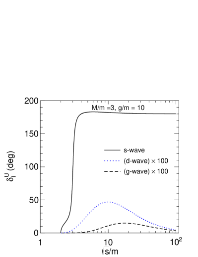
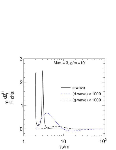
Figure 12: (Left) Variation of phase shifts with $\sqrt{s}/m$ for s-, d-, and g-waves at $g=10m<g_{S,c}$ when the resonance $S$ has mass $M=3m$. The d- and g-wave phase shifts are multiplied by a factor of 100 to make them visible. (Right) Energy dependence of s-,d-, g-wave phase shift derivatives. The d- and g-waves contributions are multiplied by a factor of 1000.

The unitarized amplitudes are given by

$$A_{k}^{U}(s)=\left[A_{k}^{-1}(s)-\Sigma(s)\right]^{-1}\text{ ,}$$ (65)

just as in Eq. (28).

Here, if the mass $M$ is sufficiently larger than the threshold $2m,$ the $s$-channel can be regarded as dominant for values of $s$ of the order of $M^{2}$. In fact, the tree-level result (neglecting $t$ and $u$ channels) reads $A_{l=0}(s)\simeq\frac{-g^{2}}{s-M^{2}}.$ Yet, the pole at $M^{2}$ is an artifact of the tree-level result. The unitarized amplitude (keeping only the $s$ channel) reads $A_{l=0}^{\text{U}}(s)\simeq\frac{-g^{2}}{s-M^{2}+g^{2}\Sigma(s)}$: the pole on the real axis moves to the complex plane ($s_{pole}\simeq M^{2}-g^{2}\operatorname{Im}\Sigma(M^{2})$) and the unitarized amplitude is simply proportional to the one-loop resumed propagator for the scalar resonance $S$ with the loop function $\Sigma(s)$ presented in Eq. (64).

The critical value of the coupling $g$ for obtaining a bound state in the s-channel is determined by

$$A_{0}^{-1}(4m^{2})-\Sigma(4m^{2})=0$$ (66)

with

$$A_{0}(s =4m^{2})=\frac{-g^{2}}{4m^{2}-M^{2}}+\frac{2g^{2}}{M^{2}}\text{ ;}$$ (67)

$$\Sigma(4m^{2}) =\frac{\sqrt{M^{2}-4m^{2}}\ln\left[-1+\frac{M\left(M+\sqrt{M^{2}-4m^{2}}\right)}{2m^{2}}\right]}{32M\pi^{2}}\text{ .}$$ (68)

Note, the fact that a critical $g$ is needed to obtain a bound state is well known in the quantum mechanical counterpart of the Yukawa interaction, e.g. Refs. Luo:2004rj ; Napsuciale:2020ehf .

The energy dependence of the unitarized phase shifts for s-, d- and g-waves and their derivatives are shown Fig. 12 for the choice $M=3m$ and $g=10m<g_{M,c}\approx 22.83m$. The s-wave phase increases rapidly near $\sqrt{s}=3m=M$ and tends towards $\approx\pi$ (from above). Compared to the s-wave, magnitudes of the d- and g-wave phase shifts are significantly smaller and hence they are multiplied by a factor of 100 to show them in this plot. At the threshold, the derivative of the s-wave phase shift is infinite, but the area under the curve is finite, hence there is no problem in evaluating thermodynamical quantities. As expected, a resonance peak is observed near $\sqrt{s}=3m=M$. The reason for this peak is the presence of the particle $S$ of mass $3m$.

Note, in Fig. 12 we display the (derivatives of the) phase shifts by using a logarithmic plot up to large values of $\sqrt{s}/m$ in order to verify that the phase shifts tend to a multiple of $\pi$. We recall, however, that inelastic channels are not taken into account. At nonzero $T$, the left parts of the plots are the relevant ones.

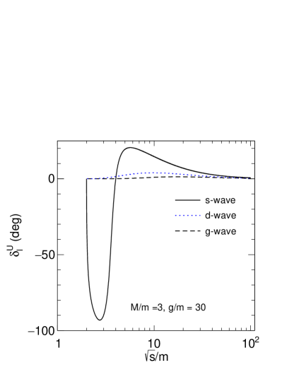
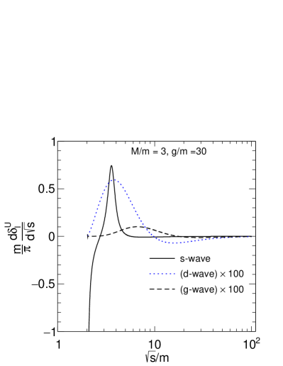
Figure 13: Similar to Fig. 12 but for $g=30m>g_{S,c}$. The d- and g-wave phase shift derivatives are multiplied by a factor of 100.

In Fig. 13 the case $g=30m>g_{M,c}$ is shown. A drastic change in the s-wave phase shift is observed, which is negative for $2m<\sqrt{s}\lessapprox 4m$, as a consequence of the presence of a bound state below the threshold. In this region, the s-wave phase shift decreases and reaches $-\pi/2$ around $\sqrt{s}/m\approx 3$, then starts increasing and becomes positive above $\sqrt{s}/m\approx 4$. It tends to zero at large $\sqrt{s}/m$. For the other two waves, the behavior is similar to Fig. 12, but somewhat larger in magnitude. The derivative of the s-wave phase shift starts from $-\infty$ at the threshold, it then increases rapidly with the increase of $\sqrt{s}/m$ and becomes positive. Around $\sqrt{s}/m\approx 3.5$ it shows a peak and starts decreasing towards zero above that. The variation of derivatives of the d- and g-waves are similar to Fig. 12, but larger in magnitude.

Finally, we refer to Appendix C for the study of causality (Wigner condition and speed of sound) for this theory. Both of them confirm that it is not violated.

IV.2 Thermodynamic properties of the system in presence of $S$

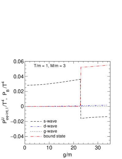
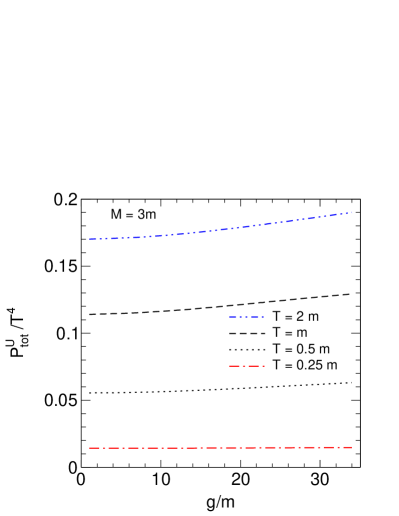
Figure 14: Left panel shows the dependence of normalized pressure of s-, d- and g-waves with $g/m$ at $T=m$ in presence of an intermediate state $S$ of mass $M=3m$ The normalized pressure of the bound state is also shown. The right panel shows the normalized total pressure at four different temperatures.

In this subsection, we discuss the thermodynamical properties of the system in presence of an intermediate state $S$ with mass $M$. The pressure is evaluated via Eq. (44), which we report for convenience:

$$P_{\varphi\varphi\text{-int}}^{U}+P_{B}=-T\int_{0}^{\infty}dx\frac{2l+1}{\pi}\sum_{l=0}^{\infty}\frac{d\delta_{l}^{U}(s=x^{2})}{dx}\int_{k}\ln\left[1-e^{-\beta\sqrt{k^{2}+x^{2}}}\right]\text{ ,}$$ (69)

which gives the overall interacting contribution. In particular, it should be stressed that:

(i) The pressure of the bound state $P_{B}$ is, as usual, nonzero only for $g>g_{M,c}.$

(ii) The contribution of the state $S$ is contained in the term $P_{\varphi\varphi\text{-int}}^{U}$; in the limit $g\rightarrow 0,$ one has

$$\frac{1}{\pi}\frac{d\delta_{0}^{U}(s=x^{2})}{dx}=\delta(x-M)\text{ ,}$$ (70)

thus $P_{\varphi\varphi\text{-int}}^{U}$ reduces to the pressure of free $S$ particles with mass $M.$ In other words, the contribution of the resonance $S$ for thermodynamic quantities is taken into account by the $\varphi\varphi\rightarrow$ $\varphi\varphi$ scattering process. In Ref. Lo:2019who this point was discussed in detail in connection with the example of the $\rho$-meson, which is not added as an independent state to the thermodynamics but is reproduced by the $\pi\pi$ phase shift’s derivative in the appropriate scattering channel.

(iii) Care is needed when $g=0.$ For this choice, the interaction contribution is, clearly, exactly zero. The state $S$ is a free field that cannot be obtained from the interaction part of the $\varphi$ field. This issue is discussed in detail in Ref. Lo:2019who : Eq. (69) and is valid for nonzero (even if infinitesimal) $g$:

$$\lim_{g\rightarrow 0}P_{\varphi\varphi\text{-int}}^{U}=P_{S,\text{free}}\neq\left(P_{\varphi\varphi\text{-int}}^{U}\right)_{g=0}=0\text{ .}$$ (71)

(iv) In connection to the discussion of Sec. III.A, the limit of small (but nonzero) $g,$ the set of asymptotic states of the theory consists of the field $\varphi$ only. The total pressure in this framework is $P_{\varphi\text{,free}}+P_{\varphi\varphi\text{-int}}^{U}$, since the state $S$ is a resonance and not an asymptotic state, no matter how small $g$ is.

Next, we turn to numerical examples for the specific choice $M=3m$. The interacting part of the normalized pressure of s-, d- and g-waves as a function of $g/m$ is shown in the left panel of Fig. 14, in which the temperature is taken as $T=m$. When $g/m$ is small, the interacting part of the pressure of the s-wave is dominated by the free particle $S$ with mass $M=3m$. As the coupling $g$ increases, the interacting part of the pressure of the s-wave contribution also increases. Up to the critical value of $g_{M,c}$ ($\approx 22.83m$), the s-wave has a positive contribution to the pressure, while it is negative above it. The interacting part of the normalized pressure of d- and g-waves are always positive, but the magnitudes are much smaller compared to that of the s-wave. In this plot, we also show the normalized pressure for the bound state (which is clearly nonzero only for $g>g_{M,c}$). As for the $\varphi^{3}$ case, the pressure of the bound state exactly compensates for the abrupt jump in the s-wave pressure at the critical value $g_{M,c}$. The normalized total pressure as a function of $g/m$ for four different $T$ is shown in the right panel of Fig. 14. Similar to Fig. 7, the total pressure is continuous in $g$, showing that also in this case the emergence of the bound state does not imply a discontinuity for the pressure.

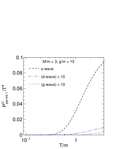
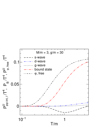
Figure 15: The left panel shows the temperature dependence of the normalized pressure for s-, g-, and d-wave at $g=10m<g_{S,c}$ in presence of an intermediate state $S$ of mass $M=3m$. The results of d- and g-waves are multiplied by a factor of 10. A similar result for $g=30m>g_{S,c}$ is shown in the right panel of this figure. The pressure of the bound state and free particles$\varphi$ are also shown.

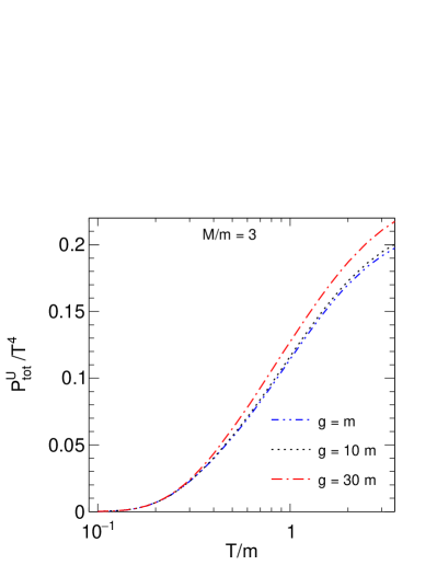
Figure 16: Variation of normalized total pressure (Eq. 47) with temperature in presence of an intermediate state of mass $M=3m$.

Next, we calculate the temperature dependence of the pressure for s-, d- and g-waves in presence of an intermediate state $S$ of mass $M=3m$. In the left panel of Fig. 15 we show the $P^{U}_{\varphi\varphi\text{-int},l}/T^{4}$ for $g/m=10$ (the d- and g-waves contributions are multiplied by 10 to make them visible). For all three waves, the normalized pressure increases and saturates at large $T/m$. The right panel of Fig. 15 shows the case $g=30m>g_{M,c}$, for which a bound state forms.

The temperature dependence of the normalized total pressure as a function of $T/m$ is shown for three values of $g$ in Fig. 16. When $g=m\ll g_{M,c}$, the attraction is very small and the resonance $S$ behaves almost like a free particle, thus basically the two free particles $\varphi$ and $S$ contribute to the pressure. At large $T$ the normalized pressure saturates to $2\pi^{2}/90\approx 0.219$. For the larger coupling $g=10m$, the state $S$ has a sizable width. As a result, the normalized total pressure is larger than the one for $g=m$. For $g=30m$, there is, in addition, also a bound state. Although the pressure of the s-wave is negative up to a certain $T/m$ (see the right panel of Fig. 15), the overall effect of the interaction for $g=30m$ is, as expected, positive.

Finally, in order to study the overall effect of the interaction, we define the following ratios:

$$\eta_{S}=\frac{P^{U}_{\text{tot}}}{P_{\varphi,\text{free}}+P_{S,\text{free}}}\text{ ,}$$ (72)

and

$$\zeta_{S}=\frac{P^{U}_{\varphi\varphi-\text{int}}+P_{B}}{P_{S,\text{free}}+P_{B}}\text{ .}$$ (73)

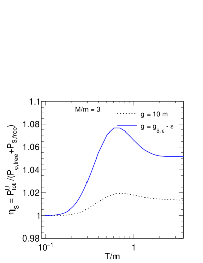
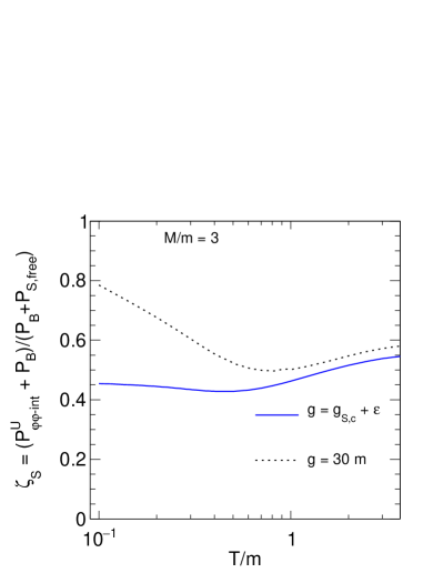
Figure 17: Dependence of the ratio $\eta$ (Eq. 72) (Left) and $\zeta$ (Eq. 73) (Right) with $T/m$ in presence of an intermediate state of mass $M=3m$ (no bound state present).

In the left panel of Fig. 17 we show $\eta_{S}$ as a function of $T/m$ at two different $g$ below the critical value $g_{M,c}$. For both cases, $\eta_{S}$ is greater than one. This implies that neglecting interaction would lead to an underestimation of the overall actual pressure. In the right panel of Fig. 17 we show $\zeta_{S}$ with $T$ for three different $g$, one just above the critical value $g_{M,c}\approx 22.83m$ and for $g=30m$. For the first case, $\zeta_{S}\approx 1$ at low temperature but, as $T/m$ increases, it decreases and reaches a minimum value $\approx 0.43$ for $T/m\approx 0.5$. With a further increase of $T/m$, the ratio $\zeta_{S}$ slightly increases and saturates at a value $\approx 0.52$. For $g=30m$, the behavior of $\zeta_{S}$ is qualitatively similar to the previous one, but at high $T/m$ it saturates to $\approx 0.55$. In both cases, neglecting the interaction would lead to a quite large overestimation of the actual results.

V Conclusions

In this work, we have investigated the role of particle interaction in a thermal gas in the context of selected scalar QFTs that contain three-leg vertices and can lead to the formation of bound states, if the attraction is strong enough. To this end, we have calculated the scattering phase shifts of the s-, d-, and g-waves using the partial wave decomposition of two-body scattering and we implemented a non-perturbative unitarized one-loop resummed approach for which the theory is a unitary, finite and well defined for a large range of the three-leg coupling constant $g$.

QFT Quantity Total pressure $P_{tot}^{U}$ Figure $\frac{g}{3!}\varphi^{3}$ $\eta$ $P_{tot}^{U}=\eta P_{\varphi,free}$ 10 (Left panel) $\frac{g}{3!}\varphi^{3}+\frac{\lambda}{4!}\varphi^{4}$ $\eta_{\lambda}$ $P_{tot}^{U}=\eta_{\lambda}P_{\varphi,free}$ 28 (Left Panel) $\frac{g}{2!}S\varphi^{2}$ $\eta_{S}$ $\begin{array}[c]{c}P_{tot}^{U}=\eta_{S}\left(P_{\varphi,free}+P_{S,free}\right)\\ =P_{\varphi,free}+\zeta_{S}P_{S,free}\end{array}$ 17 (Left panel)       

Table 1: Estimate of the interaction’s role when no bound state forms ($g$ less than the respective critical values). In each case, the expected value in absence of the interaction is one.

QFT Quantity Total pressure $P_{tot}^{U}$ Figure $\frac{g}{3!}\varphi^{3}$ $\zeta$ $P_{tot}^{U}=P_{\varphi,free}+\zeta P_{B}$ 10 (Right panel) $\frac{g}{3!}\varphi^{3}+\frac{\lambda}{4!}\varphi^{4}$ $\zeta_{\lambda}$ $P_{tot}^{U}=P_{\varphi,free}+\zeta_{\lambda}P_{B}$ 28 (Right Panel) $\frac{g}{2!}S\varphi^{2}$ $\zeta_{S}$ $P_{tot}^{U}=P_{\varphi,free}+\zeta_{S}\left(P_{S,free}+P_{B}\right)$ 17 (Right panel)       

Table 2: Estimate of the interaction’s role when a bound state forms ($g$ greater than the respective critical values). In each case, the expected value in absence of the interaction is one.

In all cases, we studied the role of the interaction and realized that, in general, it is non-negligible. Even in the case when no bound state is present, a sizable role of the interaction implies that the simple inclusion of a gas of free $\varphi$ particles maybe not be sufficient. In general, an attractive interaction (alias, a positive phase shift derivative close to threshold) implies an increase in pressure and vice-versa. This is understandable in gas at zero chemical potential determined only by the vacuum’s density of states, but it should be stressed that this is quite different from the classical case, e.g. the van der Waals gas, in which (at a fixed number of particles) a repulsion induces an increase of the pressure, see also the discussion in Ref. Yen:1997rv .

Conversely, when a bound state forms, the simple inclusion of the bound state into the thermal gas is not enough for a correct description of the pressure of the system. The derivative of the phase shift switches sign and a partial cancellation between the corresponding negative contribution of the interaction with the positive one of the bound state occurs.

We summarize our results in Table I and Table II. In table, I, the cases in which the interaction does not lead to the formation of a bound state are presented, while in Table II the cases for which a bound state appears are listed. It is then clear that the answer to our original questions about the role of the interaction as well as that of the bound state and resonances is not a simple one. The results depend on the coupling strength and eventually on other parameters and on the temperature range. Yet, as a general statement, our results show that the role of the interaction can be sizable and the consideration of a simple free gas is in most cases insufficient.

In the end, we turn back to the original question formulated in the introduction about the quite peculiar production of a bound state at a nonzero temperature in thermal models, according to which the multiplicity depends solely on the mass of the bound state but is not affect by the typically large dimension or the binding energy of the composite object. In our approach, the phase shift calculated in the vacuum is the quantity that is used to obtain the properties of the system at any temperature. Since the partition function $Z=\sum_{n}e^{-E_{n}/T}$ is determined by the energy eigenvalues $E_{n}$ calculated in the vacuum, once these are known, the quantity $Z$ is fixed for each temperature. In other words, $Z$ is solely fixed by vacuum physics. In our work, the sum over the states is replaced by an integral over the derivatives of the spectral function, but the basic idea is the same since the pressure is still determined by vacuum quantities. One may then speculate that the production (alias the multiplicity) of a bound state is not related to the dimension of the composite objects but is solely controlled by the corresponding thermal integral as thermal models suggest, but one needs to investigate this issue more in detail in the future.

As an additional important outlook, we mention the extension of the present work to particles with spins (both bosons and fermions), with particular attention to the study of nuclei as bound states of nucleons, the easiest of such systems being the deuteron, as well as to resonances that do not fit into the quarkonium picture, such as the famous exotic meson $X(3872)$.

Acknowledgments: The authors thank W. Broniowski and S. Mrówczyński for useful discussions about the thermodynamics of bound states and A. Pilloni for scattering issues. F.G. acknowledges financial support from the Polish National Science Centre NCN through OPUS project no. 2019/33/B/ST2/00613. S.S. acknowledges financial support from the Ulam Scholarship of the Polish National Agency for Academic Exchange (NAWA) with agreement no: PPN/ULM/2019/1/00093/U/00001.

Appendix A Brief recall of the phase shift formula

In this Appendix, for completeness, we recall a simple QM-based justification of the phase shift formula Florkowski:2010zz that shows how it is linked to the density of states. The radial wave function with angular momentum $l$ of a particle scattered by central potential $U(r)$ is

$$\psi_{l}(r)\propto\sin[kr-l\pi/2+\delta_{l}]\text{ ,}$$ (74)

where $k$ is the length of the three-momentum and $\delta_{l}$ is the phase shift due to the interaction with the potential.

If we confine our system into a sphere of radius $R,$ the condition $kR-l\pi/2+\delta_{l}=n\pi$ with $n=0,1,2,..$ holds because $\psi_{l}(r)$ must vanish at the boundary. Conversely, the number of states $n_{0}$ when $k$ belongs to the range $(0,k_{0})$ is given by $n_{0}=\left(k_{0}R-l\pi/2+\delta_{l}\right)/\pi.$ Then, the density of states that one can place between $k$ and $k+dk$ is given by

$$\frac{dn_{l}}{dk}=\frac{R}{\pi}+\frac{1}{\pi}\frac{d\delta_{l}}{dk}\text{ ,}$$ (75)

where the first term describes the density of states $\frac{dn_{l}^{free}}{dk}$ in absence of interactions, while the second term $\frac{1}{\pi}\frac{d\delta_{l}}{dk}$ describes the effect of the interacting potential. When translating these results from QM to QFT, we replace the momentum $k$ by the invariant mass $x=\sqrt{s}.$ For instance, in the case of the $\varphi^{3}$-QFT and for $l=0$ and no bound state, one has:

$$\frac{dn_{0}}{dx}=\delta(x-m)+\frac{1}{\pi}\frac{d\delta_{0}}{dx}\text{ ,}$$ (76)

where the phase shift is nonzero for $x\geq 2m.$ If a bound state in the s-wave channel forms, one has:

$$\frac{dn_{0}}{dx}=\delta(x-m)+\delta(x-M_{B})+\frac{1}{\pi}\frac{d\delta_{0}}{dx}\text{ .}$$ (77)

Indeed, the formal extension outlined in Sec. II.C amounts to

$$\frac{dn_{0}}{dx}=\frac{1}{\pi}\frac{d\delta_{0}^{\text{(extended)}}}{dx}\text{ .}$$ (78)

Appendix B Loop function for small but nonzero $\varepsilon$

The loop function $\Sigma$ is, in general, a complex function which (on its first Riemann sheet) is regular everywhere apart from a cut that starts from a certain threshold $s_{th}$ to $\infty.$ Upon considering (at first) the case without subtractions, its general form as a function of the complex variable $z$ is given by:

$$\Sigma(z)=-\frac{1}{\pi}\int_{s_{th}}^{\infty}ds^{\prime}\frac{f(s^{\prime})}{z-s^{\prime}}\text{ ,}$$ (79)

which is well-defined for each $z\in\mathbb{C}$ except for the cut $(s_{th},\infty).$ Above, $f(s)$ is a well-defined function (that can be continued to the whole complex plane: $f(s)\rightarrow f(z);$ this is necessary to go to the second Riemann sheet, yet we will not deepen this matter here). In our specific case (see also below) we have:

$$f(s)=\frac{\sqrt{s-s_{th}}}{32\pi\sqrt{s}}\text{ , }s_{th}=4m^{2}\text{ .}$$ (80)

When convergence is not guaranteed (as for the $f(s)$ above), subtractions are necessary. For instance, with two subtractions (as in the main text) one has

$$\Sigma_{\text{2S}}(z)=-\frac{1}{\pi}(z-s_{1})(z-s_{2})\int_{s_{th}}^{\infty}ds^{\prime}\frac{f(s^{\prime})}{\left(z-s^{\prime}\right)\left(s^{\prime}-s_{1}\right)(s^{\prime}-s_{2})}\text{ ,}$$ (81)

for $s_{1,2}<s_{th}.$ It is, however, important to stress that subtractions do not affect the behavior of the imaginary part that we shall describe below. We shall then omit them in the following.

As it is common (being an outcome of the Feynman prescription, as we show explicitly below in the case of scalar QFT) the cut is moved to the negative axis by a small amount, leading to:

$$\Sigma(z)=-\frac{1}{\pi}\int_{s_{th}}^{\infty}ds^{\prime}\frac{f(s^{\prime})}{z-s^{\prime}+i\varepsilon}]text{.}$$ (82)

Namely, the cut is now located at $(s_{th}-i\varepsilon,\infty-i\varepsilon),$ where $\varepsilon$ is an infinitesimal (but nonzero) number.

Since the cut is below the real axis, we can now consider $z=s\in$ $\mathbb{R}$ (including $(s_{th},\infty)$). The imaginary part for $z=s\in$ $\mathbb{R}$ takes the form:

$$\operatorname{Im}\Sigma(z=s)=\int_{s_{th}}^{\infty}ds^{\prime}f(s^{\prime})\frac{1}{\pi}\frac{\varepsilon}{(s-s^{\prime})^{2}+\varepsilon^{2}}.$$ (83)

It is useful to distinguish three regions for this object.

(i) For $s-s_{th}\ll-\varepsilon,$ the previous expression reads:

$$\operatorname{Im}\Sigma(z=s)=\varepsilon\int_{s_{th}}^{\infty}ds^{\prime}f(s^{\prime})\frac{1}{\pi}\frac{1}{(s-s^{\prime})^{2}}=\varepsilon h(s)\sim\varepsilon$$ (84)

where $h(s)$ is a certain finite function for the considered range of interest; thus $\operatorname{Im}\Sigma(z=s)$ is an infinitesimal (but nonzero) quantity for a non-vanishing $\varepsilon$.

(ii) For $-\varepsilon\lesssim s-s_{th}\lesssim\varepsilon$ (for $s$ close to threshold), one has:

$$\int_{s_{th}}^{\infty}ds^{\prime}f(s^{\prime})\frac{1}{\pi}\frac{\varepsilon}{(s-s^{\prime})^{2}+\varepsilon^{2}}\sim\sqrt{\varepsilon}\text{ ,}$$ (85)

as can be seen by a lengthy but explicit calculation. A simple verification can be obtained by setting $s=s_{th}$ and by approximating $f(s)$ as $f(s)\simeq c\sqrt{s-s_{th}}$ (valid close to threshold, where the dominant part of the integral comes from). In this case, the integral reads $c\sqrt{\varepsilon/2}$ (with $c$ being a positive constant).

(iii) For $s-s_{th}\gg\varepsilon,$ the quantity $\frac{1}{\pi}\frac{\varepsilon}{(s-s^{\prime})^{2}+\varepsilon^{2}}$ can be safely replaced by $\delta(s-s^{\prime})$ when $\varepsilon$ is sufficiently small, leading to

$$\operatorname{Im}\Sigma(z=s)=f(s)\text{ .}$$ (86)

By going to the the next order in $\varepsilon$, one has

$$\operatorname{Im}\Sigma(z=s)=f(s)+\varepsilon r(s),$$ (87)

where $r(s)$ is a certain finite function given by $r(s)=\lim_{\varepsilon\rightarrow 0^{+}}\int_{s_{th}}^{\infty}ds^{\prime}f(s^{\prime})\frac{1}{\pi}\frac{(s-s^{\prime})^{2}-\varepsilon^{2}}{[(s-s^{\prime})^{2}+\varepsilon^{2}]^{2}}$. [Note, the function $r(s)$ can be calculated by taking the Fourier transform of the Lorentzian $\delta$-function, which then leads to $r(s)=\int_{-\infty}^{+\infty}\frac{dq}{\sqrt{2\pi}}(-\left|q\right|)F(q,s)$, where $F(q,s)=\int_{s_{th}}^{\infty}\frac{ds^{\prime}}{\sqrt{2\pi}}f(s^{\prime})e^{-iq\cdot(s^{\prime}-s)}$.]

Finally, in the transition regions between (i) and (ii) the small quantity rises from $\varepsilon$ to $\sqrt{\varepsilon},$ while between (ii) and (iii) from $\sqrt{\varepsilon}$ to a finite number.

Thus, we may summarize the outcome as

$$\operatorname{Im}\Sigma(z=s)\left\{\begin{array}[]{c}\epsilon\propto\varepsilon\text{ for }s-s_{th}\ll-\varepsilon\\ \epsilon\propto\sqrt{\varepsilon}\text{ for }-\varepsilon\lesssim s-s_{th}\lesssim\varepsilon\\ f(s)+\epsilon\text{ with }\epsilon\propto\varepsilon\text{ for }s-s_{th}\gg\varepsilon\end{array}\right.\text{ ,}$$ (88)

whose schematic and illustrative behavior is reported in Fig.18. In particular, one may appreciate that the function is continuous and very small (but nonzero) below threshold . By expressing the part below threshold by an infinitesimal quantity $\epsilon$ (to be distinguished from the original $\varepsilon$) we obtain Eq. (26) presented in the main text. Of course, in this respect $\epsilon$ is in general a rather complicated function of $\varepsilon$ and $s$, but the important point here is that it is a very small number that approaches $0$ when $\varepsilon$ goes to zero.

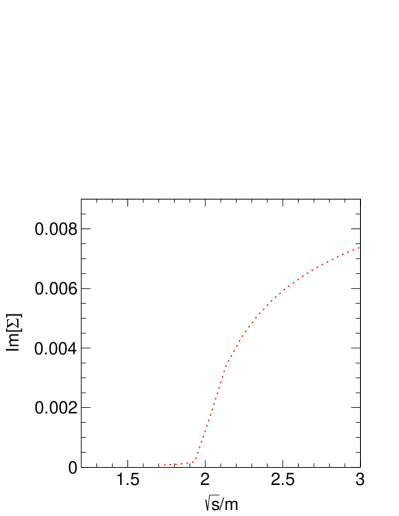
Figure 18: Energy dependence of the function Im$\Sigma(z=s)$ for a nonzero $\varepsilon$ (Eq. 88).

As a final step, we show how the loop function of Eq. (79) emerges from the standard Feynman rules. We start with the very well known expression of the loop of two scalar particles with mass $m$ as a function of the overall momentum $p^{2}$ ($p$ being the overall momentum of the two-particle system):

$$-i\Sigma(p^{2})=\frac{1}{2}\int\frac{d^{2}q}{(2\pi)^{4}}\frac{i}{(p/2+q)^{2}-m^{2}+i\frac{\varepsilon}{2}}\frac{i}{(p/2-q)^{2}-m^{2}+i\frac{\varepsilon}{2}}$$ (89)

where the infinitesimal quantity $\varepsilon$ is chosen according to the Feynman prescription (roughly speaking, positive energy solutions propagate forward in time and negative energy solutions backward). In other words, we add a small imaginary part to the particle $\varphi,$ thus making itself unstable. The factor $1/2$ in front of the integral is due to identical particles. The choice of $\varepsilon/2$ is for future convenience. Taking for simplicity $p=(\sqrt{s},\mathbf{0})$ (rest frame for the colliding particles), we have:

$$\Sigma(s)=-i\frac{1}{2}\int\frac{d^{4}q}{(2\pi)^{4}}\frac{1}{(\sqrt{s}/2+q^{0})^{2}-\mathbf{q}^{2}-m^{2}+i\frac{\varepsilon}{2}}\frac{1}{(\sqrt{s}/2-q^{0})^{2}-\mathbf{q}^{2}-m^{2}+i\frac{\varepsilon}{2}}$$ (90)

The integral over $q^{0}$ can be performed by a standard residuum calculus (here, we keep track of the $\varepsilon$, since this is important for our purposes):

$$\Sigma(s)=-\frac{1}{2}\int\frac{d^{3}q}{(2\pi)^{2}}\frac{1}{E-i\frac{\varepsilon}{4E}}\frac{1}{s-4E^{2}+i\varepsilon}\text{ .}$$ (91)

with $E=\sqrt{\mathbf{q}^{2}+m^{2}}$ (note, formally $\varepsilon$ has dimension $[$Energy${}^{2}]$). Since $E>0$ (we do not consider the case of zero masses), the previous expression simplifies as

$$\Sigma(s)=-\frac{1}{2}\int\frac{d^{3}q}{(2\pi)^{2}}\frac{1}{E}\frac{1}{s-4E^{2}+i\varepsilon}\text{ .}$$ (92)

As a last step, upon introducing $s^{\prime}=4E^{2}$ as a variable, we get

$$\Sigma(s)=-\frac{1}{2\cdot 16\pi^{2}}\int_{s_{th}=4m^{2}}^{\infty}ds^{\prime}\frac{\sqrt{s^{\prime}-4m^{2}}}{\sqrt{s^{\prime}}}\frac{1}{s-s^{\prime}+i\varepsilon}\text{ }$$ (93)

which coincides with the loop of Eq. (79).

Appendix C $N/D$ unitarization scheme

In this Appendix, we present an alternative unitarization scheme for the case of the $\varphi^{3}$-QFT. To this end, we choose the well-known $N/D$ scheme Frazer:1969euo ; Hayashi:1967bjx ; Gulmez:2016scm ; Oller:2020guq ; Cahn:1983vi ; Mai:2022eur ; Giacosa:2021brl . At the lowest order, the unitarized amplitude reads Cahn:1983vi ; Gulmez:2016scm

$$A_{l}^{N/D}(s)=\frac{N_{l}(s)}{D_{l}(s)},$$ (94)

where $N_{l}(s)=A_{l}(s)$ (tree-level result, see Sec. II), and the denominator takes the form

$$D_{l}(s)=1-\dfrac{(s-m^{2})}{\pi}\int_{4m^{2}}^{\infty}\frac{\rho(s_{1})N_{l}(s_{1})}{(s_{1}-s-i\varepsilon)(s_{1}-m^{2})}ds_{1}\text{ .}$$ (95)

The right-hand-cut is contained in $D_{l}(s)$ ($\operatorname{Im}D_{l}=-\rho(s)N_{l}(s)\theta(s-4m^{2})$, while the left-hand cut is contained in $N_{l}(s).$ Here, a single subtraction (at the particle pole $s=m^{2}$) is implemented: this is enough to guarantee convergence and, within this method, there is no problem with emerging ghosts.

Quite interestingly, the once-subtracted on-shell unitarization scheme is obtained if we approximate $D_{l}(s)$ as

$$D_{l}(s)\approx 1-N_{l}(s)\dfrac{(s-m^{2})}{\pi}\int_{4m^{2}}^{\infty}\frac{\rho(s_{1})}{(s_{1}-s-i\varepsilon)(s_{1}-m^{2})}ds_{1}\text{ .}$$ (96)

Roughly speaking, the quantity $N_{l}(s)$ is taken outside the integral. Yet, as discussed in the main text, this scheme leads to issues related to the emergence of a ghost pole.

As a consequence of Eq. (95), the bound state in the $N/D$ approach, in any given wave, is realized by $D_{l}(s)=0$ for $s<4m^{2},$ but only the case $l=0$ is relevant for our purposes. In the present unitarization, the bound state mass (if existent) belongs to the interval $(m,2m)$, thus the range is different from the one of the on-shell approximation $(\sqrt{3}m,2m)$. This aspect shows explicitly what was discussed in Secs. II.B and II.C: different unitarization schemes typically agree when the bound state mass is not too far from the threshold, but may be quite different when the coupling constant becomes too large.

Let us now discuss in more detail the s-wave. The numerator reads explicitly

$$N_{0}(s)=A_{0}(s)=\frac{-g^{2}}{s-m^{2}}+2g^{2}\frac{\ln\left[1-\frac{s-4m2}{m^{2}}\right]}{s-4m^{2}}\text{ ,}$$ (97)

thus the left-hand cut with branch point at $s=3m^{2}$ as well as a single-particle pole is encoded in the numerator. The denominator $D_{0}(s)$ can be then evaluated numerically from Eq. (95).

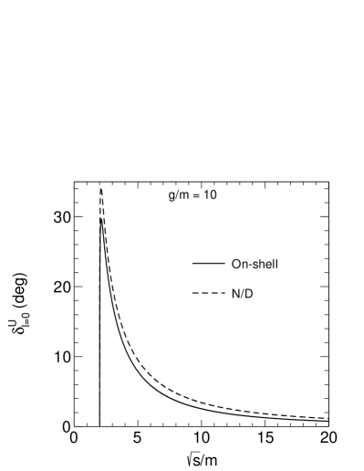
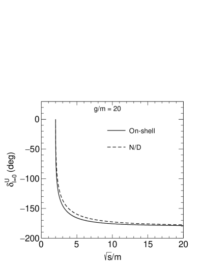
Figure 19: Comparisons of the energy dependence of s-wave phase shifts in two different unitarization approaches. The left panel is for $g/m=10$ and the right panel is for $g/m=20$.

in Fig. 19 we present the s-wave phase shift for $g/m=10$ (no bound state in both $N/D$ and on-shell schemes) and $g/m=20$ (bound state present in both approaches), where it is compared to the result of the on-shell scheme. As it is visible, both results are very similar.

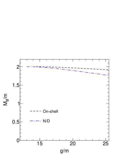
Figure 20: Comparisons of bound state masses in two different unitarization approaches.

Next, the critical value of $g_{c}$ for obtaining a bound state reads $g_{c}^{N/D}/m=13.0177,$ that compares well to $g_{c}/m=14.4551$ discussed in Sec. II.B. The behavior of the mass of the bound state as a function of $g$ is depicted in Fig. 20 for both approaches, displaying a comparable behavior.

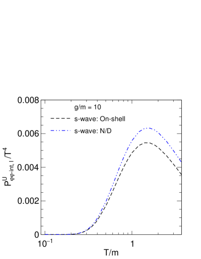
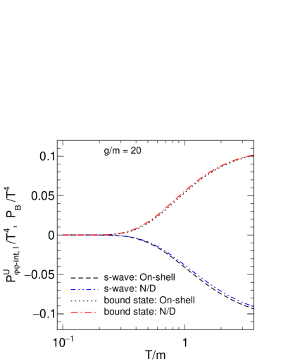
The l

Figure 21: Left panel compares the temperature dependence of the normalized pressure for s-wave in two different unitarization approaches for $g=10m$. The right panel shows a similar plot for $g=20m$ where the bound state contribution is also included.

Finally, in Fig. 21 we show the s-wave contribution of the pressure for both unitarization schemes. Also, in this case, the results are numerically close to each other for the considered range of temperatures.

In conclusion, the results of the $N/D$ approach confirm qualitatively the ones shown in the main part of the manuscript. Of course, one could go beyond the lowest order in $N/D$ and/or also attempt other unitarizations. This task is left for the future.

Appendix D Causality of the $\varphi^{3}$ and $S\varphi^{2}$ QFTs

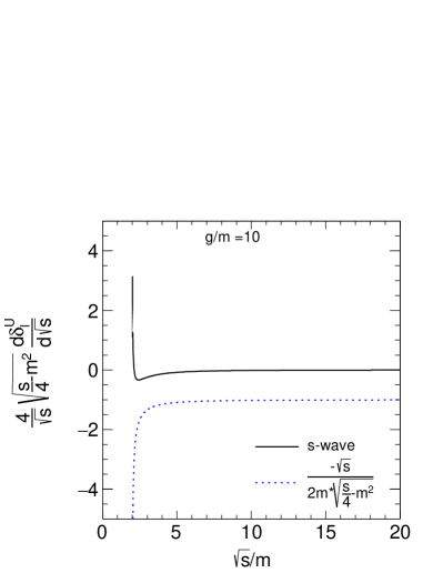
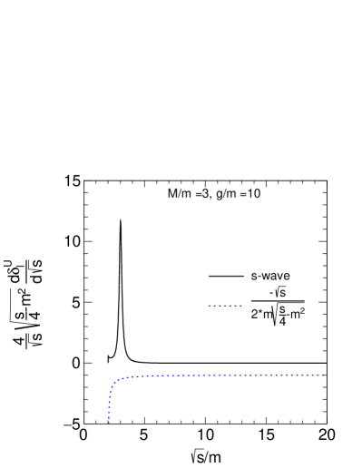
Figure 22: Wigner’s causality condition for $\varphi^{3}$ (left) type interaction and $S\varphi^{2}$ (right) type interaction.

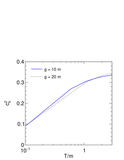
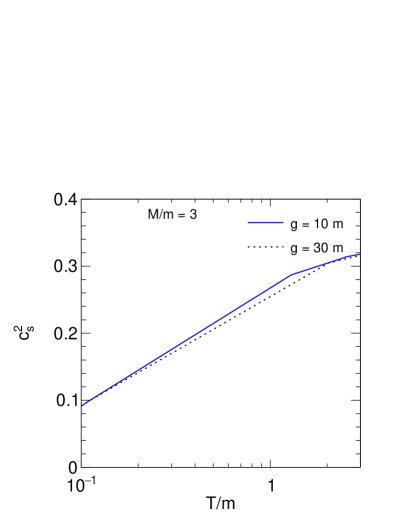
Figure 23: Temperature dependence of $c_{s}^{2}$ for $\varphi^{3}$ (left) type interaction and $S\varphi^{2}$ (right) type interaction.

In this Appendix, we verify that causality is fulfilled for the $\varphi^{3}$ and $S\varphi^{2}$ QFTs by evaluating the Wigner condition for the phase shifts in the vacuum as well and as the speed of sound $c_{s}$ in the medium.

In Fig. 22 we show the Wigner’s causality condition of Eq. 42 (see Ref. Boglione:2002vv ) for $\varphi^{3}$ and the $S\varphi^{2}$ interactions at $g/m=10$, which show that this condition is always fulfilled. Test with different values of $g$ confirms this result.

Next, for both theories, we show in Fig. 23 the temperature dependence of the square of the speed of sound $c_{s}^{2}$ (Eq. 53), which is less than one in the whole considered range of the $T/m$.

Appendix E Adding a four-leg interaction

In this Appendix, we show how the results change when adding an interaction term proportional to $\varphi^{4}$:

$$\mathcal{L}=\frac{1}{2}\left(\partial_{\mu}\varphi\right)^{2}-\frac{1}{2}m^{2}\varphi^{2}-\frac{g}{3!}\varphi^{3}-\frac{\lambda}{4!}\varphi^{4},$$ (98)

whose tree-level scattering amplitude reads

$$A(s,t,u) =-\lambda-\frac{g^{2}}{s-m^{2}+i\epsilon}-\frac{g^{2}}{t-m^{2}+i\epsilon}-\frac{g^{2}}{u-m^{2}+i\epsilon}\text{ .}$$ (99)

Only the s-wave amplitude is modified by including the $\varphi^{4}$ term, hence we concentrate on the lowest wave. The new expression for the tree-level s-wave amplitude reads:

$$A_{0}(s)=\frac{1}{2}\int_{-1}^{+1}d\xi A(s,\theta)=-\lambda-\frac{g^{2}}{s-m^{2}}+2g^{2}\frac{\ln\left[1+\frac{s-4m^{2}}{m^{2}}\right]}{s-4m^{2}}\text{ ,}$$ (100)

out of which the tree-level scattering length takes the form:

$$a_{0}^{\text{SL}}=\frac{1}{2}\frac{A_{0}(s=4m^{2})}{8\pi\sqrt{4m^{2}}}=\frac{-\lambda}{32\pi m}+\frac{1}{32\pi m}\frac{5g^{2}}{3m^{2}}\text{ .}$$ (101)

The loop function allows calculating the unitarized amplitudes in the $s$-channel as:

$$A_{0}^{U}(s)=\left[A_{0}^{-1}(s)-\Sigma(s)\right]^{-1}\text{ ,}$$ (102)

where $\Sigma(s)$ is the loop function reported in Eq. (24), see also Ref. Giacosa:2021brl . The unitarized scattering length reads:

$$a_{0}^{U,\text{SL}} =a_{0}^{U}(s=4m^{2})=\frac{1}{2}\frac{1}{16\pi m}\frac{1}{A_{0}^{-1}(4m^{2})-\Sigma(4m^{2})}=\frac{1}{32\pi m}\frac{1}{\left[-\lambda+\frac{5g^{2}}{3m^{2}}\right]^{-1}-\frac{1}{64\sqrt{3}\pi}\text{.}}\text{.}$$ (103)

For a certain fixed value of $\lambda,$ the new critical value of $g$ is given by:

$$-\lambda+\frac{5g^{2}}{3m^{2}}=64\sqrt{3}\pi\text{ , }g_{\lambda,c}^{2}=g_{c}^{2}+\frac{3m^{2}}{5}\lambda\text{ ,}$$ (104)

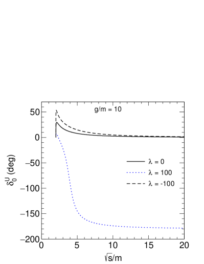
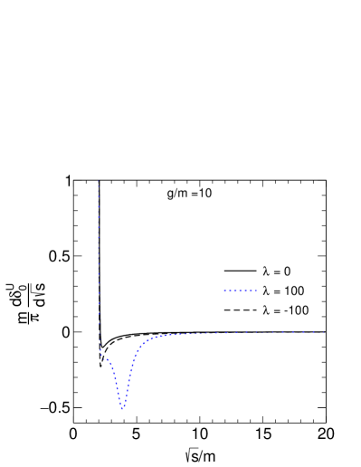
Figure 24: (Left) The plot of the s-wave phase shift (using Eqs. 100 and 30) as a function of $\sqrt{s}/m$ at $g=10m$ when the additional $\varphi^{4}$-term is present. (Right) The corresponding derivatives with respect to $\sqrt{s}/m$.

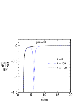
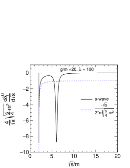
Figure 25: Left and middle panels: same as Fig. 24 but for $g=20m$. Right panel: Wigner condition.

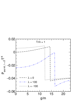
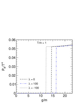
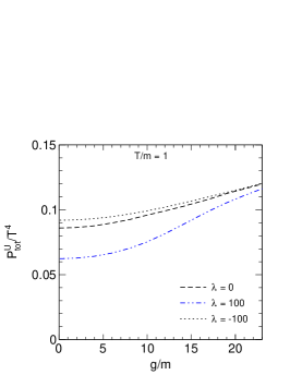
Figure 26: Normalized s-wave contribution to the pressure (left) (Eq. 44) and bound state (middle) (Eq. 46) as a function of $g/m$ when the additional $\varphi^{4}$-term is present. Right: total pressure as a function of $g$.

In Fig. 24 we show the s-wave phase shift as a function of $\sqrt{s}/m$ for $g/m=10$ and for three different values of $\lambda$ ($\lambda=0$ as a reference, $\lambda=100$ (repulsive) for which $g_{\lambda,c}/m\approx 16.4$, and $\lambda=-100$ (attractive) for which $g_{\lambda,c}/m\approx 12.2$, thus no bound state forms in any of these cases). Interestingly, the case $\lambda=-100$ is similar to $\lambda=0$. Yet, the situation is completely different for $\lambda=100$, where the phase shift decreases and saturates to $-\pi$ at large energies.

The figure 25is obtained for $g=20m>g_{\lambda,c}$, for which a bound state forms. Also here, the case $\lambda=-100$ is similar to $\lambda=0$. Quite different behavior is observed in the case of $\lambda=100$ where at large $\sqrt{s}/m$ the phase shift saturates to $-2\pi$. The phase shift derivatives are plotted in the right panel. Interestingly, a deep near $\sqrt{s}/m=6$ is observed for $\lambda=100$.

The case $\lambda>0$ needs some care. There is a certain value of $s=s_{0}\simeq 6m^{2}$ for which the tree-level and the unitarized amplitudes vanish: $A(s_{0})=A^{U}(s_{0})=0$. At this point, the attractive $\varphi^{3}$-term cancels the repulsive $\varphi^{4}$-term. For this energy, $\delta^{U}(x=\sqrt{s_{0}})=n\pi$, where the choice $n=-1$ is dictated by the requirement of continuity. Indeed, the dip in Fig. 25 corresponds to the $s_{0}$ value. For $s>s_{0}$ the $\varphi^{4}$-term becomes dominant and the phase shift tends slowly to $-2\pi$. Yet, the Wigner condition of Eq. (42) is violated around $s_{0}$, as the right plot of Fig. 25 shows. This violation takes place at energy for which inelastic channels and higher waves are also expected to be relevant and is a further indication that a limited range of $s$ should be considered. Indeed, the proper treatment of inelasticities and/or the use of other unitarization approaches could solve this issue.

Next, we turn to the pressure. In the left panel of Fig. 26 we show the normalized s-wave interacting pressure as a function of $g/m$ for three values of $\lambda$ and for $T/m=1$. Note, the discontinuity in the s-wave pressure corresponds to $g_{\lambda,c}$: the larger $\lambda$, the larger $g_{\lambda,c}$ needed to form a bound state, see Eq. (104). The normalized pressure of the bound state is shown in the middle panel of Fig. 26, which -just as before- starts abruptly at $g_{\lambda,c}$. The total pressure is, as expected, continuous in $g$, which is shown in the right panel.

The temperature dependence of total normalized pressure for $g=10m$ and $20m$ is shown in Fig. 27 (left and middle plots). Note, for $\lambda=100$ total pressure is significantly reduced w.r.t. the case $\lambda=0$.

In the right panel, we present the speed of sound for $\lambda=100$. It overshoots one at about $T/m\sim 3.3$, which then represents a clear upper limit for the present model. As mentioned above, other effects are expected to be relevant for these temperatures.

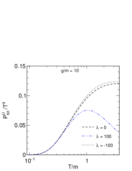
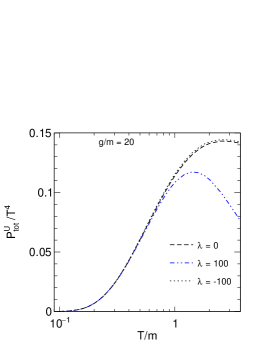
Figure 27: Left: Normalized total pressure (Eq. 47) as function of $T/m$ at different $\lambda$ and for $g=10m$. Middle: the same for $g=20m$. Right: Speed of sound as function of $T$.

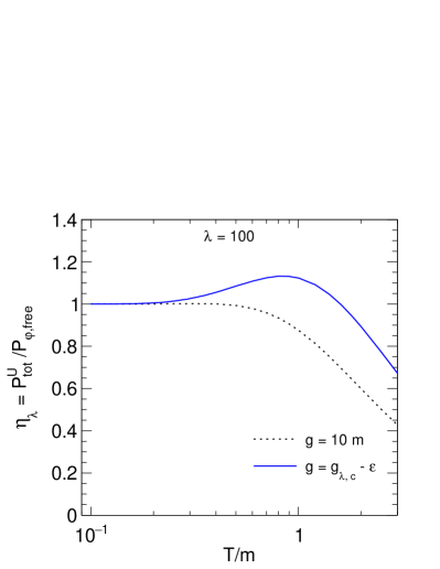
Figure 28: Temperature dependence of the ratios $\eta_{\lambda}$ and $\zeta_{\lambda}$ for $\lambda=100$ (Eq. 105) for different values of $g$.

In the end, we define quantities similar to Eqs. 54 and 55 as:

$$\eta_{\lambda}=\frac{P^{U}_{\text{tot}}}{P_{\varphi\text{,free}}}\text{ ,}\zeta_{\lambda}=\frac{P^{U}_{\varphi\varphi-\text{int}}+P_{B}}{P_{B}}\text{ ,}$$ (105)

which are used to quantify the effect of the interaction. Figure 28 shows the variation of $\eta_{\lambda}$ and $\zeta_{\lambda}$ with $T/m$ at $\lambda=100$ and for different $g$ values. The quantity $\eta_{\lambda}$ is close to one at low $T$, then it increases and reaches a maximum: the further decrease takes place in a region of $T$ where caution is needed. The quantity $\zeta_{\lambda}$ implies a partial cancellation of the single bound state contribution, in agreement with the other QFTs studied in this work.

References

- (1) V. T. Cocconi, T. Fazzini, G. Fidecaro, M. Legros, N. H. Lipman, and A. W. Merrison, Mass Analysis of the Secondary Particles Produced by the 25-Gev Proton Beam of the Cern Proton Synchrotron, Phys. Rev. Lett. 5 (1960) 19–21.
- (2) STAR Collaboration, B. I. Abelev et al., Observation of an Antimatter Hypernucleus, Science 328 (2010) 58–62, [arXiv:1003.2030].
- (3) STAR Collaboration, H. Agakishiev et al., Observation of the antimatter helium-4 nucleus, Nature 473 (2011) 353, [arXiv:1103.3312]. [Erratum: Nature475,412(2011)].
- (4) ALICE Collaboration, J. Adam et al., Production of light nuclei and anti-nuclei in pp and Pb-Pb collisions at energies available at the CERN Large Hadron Collider, Phys. Rev. C93 (2016), no. 2 024917, [arXiv:1506.08951].
- (5) STAR Collaboration, J. Adam et al., Measurement of the mass difference and the binding energy of the hypertriton and antihypertriton, Nature Phys. 16 (2020), no. 4 409–412, [arXiv:1904.10520].
- (6) ALICE Collaboration, S. Acharya et al., Production of (anti-)3He and (anti-)3H in p-Pb collisions at = 5.02 TeV, Phys. Rev. C101 (2020), no. 4 044906, [arXiv:1910.14401].
- (7) ALICE Collaboration, S. Acharya et al., (Anti-)Deuteron production in pp collisions at TeV, arXiv:2003.03184.
- (8) A. Esposito, A. L. Guerrieri, F. Piccinini, A. Pilloni, and A. D. Polosa, Four-Quark Hadrons: an Updated Review, Int. J. Mod. Phys. A 30 (2015) 1530002, [arXiv:1411.5997].
- (9) LHCb Collaboration, R. Aaij et al., Observation of a narrow pentaquark state, , and of two-peak structure of the , Phys. Rev. Lett. 122 (2019), no. 22 222001, [arXiv:1904.03947].
- (10) P. J. Siemens and J. I. Kapusta, Evidence for a soft nuclear matter equation of state, Phys. Rev. Lett. 43 (1979) 1486–1489.
- (11) A. Andronic, P. Braun-Munzinger, J. Stachel, and H. Stocker, Production of light nuclei, hypernuclei and their antiparticles in relativistic nuclear collisions, Phys. Lett. B697 (2011) 203–207, [arXiv:1010.2995].
- (12) A. Andronic, P. Braun-Munzinger, K. Redlich, and J. Stachel, The statistical model in Pb-Pb collisions at the LHC, Nucl. Phys. A904-905 (2013) 535c–538c, [arXiv:1210.7724].
- (13) J. Cleymans, S. Kabana, I. Kraus, H. Oeschler, K. Redlich, and N. Sharma, Antimatter production in proton-proton and heavy-ion collisions at ultrarelativistic energies, Phys. Rev. C84 (2011) 054916, [arXiv:1105.3719].
- (14) P. G. Ortega, D. R. Entem, F. Fernandez, and E. Ruiz Arriola, Counting states and the Hadron Resonance Gas: Does X(3872) count?, Phys. Lett. B781 (2018) 678–683, [arXiv:1707.01915].
- (15) P. G. Ortega and E. Ruiz Arriola, Is X(3872) a bound state?, Chin. Phys. C 43 (2019), no. 12 124107, [arXiv:1907.01441].
- (16) S. T. Butler and C. A. Pearson, Deuterons from High-Energy Proton Bombardment of Matter, Phys. Rev. 129 (1963) 836–842.
- (17) A. Schwarzschild and C. Zupancic, Production of Tritons, Deuterons, Nucleons, and Mesons by 30-GeV Protons on A-1, Be, and Fe Targets, Phys. Rev. 129 (1963) 854–862.
- (18) H. H. Gutbrod, A. Sandoval, P. J. Johansen, A. M. Poskanzer, J. Gosset, W. G. Meyer, G. D. Westfall, and R. Stock, Final State Interactions in the Production of Hydrogen and Helium Isotopes by Relativistic Heavy Ions on Uranium, Phys. Rev. Lett. 37 (1976) 667–670.
- (19) H. Sato and K. Yazaki, On the coalescence model for high-energy nuclear reactions, Phys. Lett. 98B (1981) 153–157.
- (20) S. Mrowczynski, On the neutron proton correlations and deuteron production, Phys. Lett. B277 (1992) 43–48.
- (21) L. P. Csernai and J. I. Kapusta, Entropy and Cluster Production in Nuclear Collisions, Phys. Rept. 131 (1986) 223–318.
- (22) S. Mrowczynski, Production of light nuclei in the thermal and coalescence models, Acta Phys. Polon. B48 (2017) 707, [arXiv:1607.02267].
- (23) S. Bazak and S. Mrowczynski, vs. and production of light nuclei in relativistic heavy-ion collisions, Mod. Phys. Lett. A33 (2018), no. 25 1850142, [arXiv:1802.08212].
- (24) Z.-J. Dong, G. Chen, Q.-Y. Wang, Z.-L. She, Y.-L. Yan, F.-X. Liu, D.-M. Zhou, and B.-H. Sa, Energy dependence of light (anti)nuclei and (anti)hypertriton production in the Au-Au collision from to 5020 GeV, Eur. Phys. J. A54 (2018), no. 9 144, [arXiv:1803.01547].
- (25) K.-J. Sun and L.-W. Chen, Production of and in central Pb+Pb collisions at = 2.76 TeV within a covariant coalescence model, Phys. Rev. C94 (2016), no. 6 064908, [arXiv:1607.04037].
- (26) K.-J. Sun, L.-W. Chen, C. M. Ko, J. Pu, and Z. Xu, Light nuclei production as a probe of the QCD phase diagram, Phys. Lett. B781 (2018) 499–504, [arXiv:1801.09382].
- (27) A. Polleri, J. P. Bondorf, and I. N. Mishustin, Effects of collective expansion on light cluster spectra in relativistic heavy ion collisions, Phys. Lett. B419 (1998) 19–24, [nucl-th/9711011].
- (28) S. Mrówczyński and P. Słoń, Hadron–Deuteron Correlations and Production of Light Nuclei in Relativistic Heavy-ion Collisions, Acta Phys. Polon. B 51 (2020), no. 8 1739–1755, [arXiv:1904.08320].
- (29) S. Bazak and S. Mrowczynski, Production of and correlation function in relativistic heavy-ion collisions, Eur. Phys. J. A 56 (2020), no. 7 193, [arXiv:2001.11351].
- (30) P. Danielewicz and G. F. Bertsch, Production of deuterons and pions in a transport model of energetic heavy ion reactions, Nucl. Phys. A533 (1991) 712–748.
- (31) D. Oliinychenko, L.-G. Pang, H. Elfner, and V. Koch, Microscopic study of deuteron production in PbPb collisions at via hydrodynamics and a hadronic afterburner, Phys. Rev. C99 (2019), no. 4 044907, [arXiv:1809.03071].
- (32) S. Samanta and F. Giacosa, QFT treatment of a bound state in a thermal gas, Phys. Rev. D 102 (2020) 116023, [arXiv:2009.13547].
- (33) R. Dashen, S.-K. Ma, and H. J. Bernstein, S Matrix formulation of statistical mechanics, Phys. Rev. 187 (1969) 345–370.
- (34) R. Venugopalan and M. Prakash, Thermal properties of interacting hadrons, Nucl. Phys. A 546 (1992) 718–760.
- (35) W. Broniowski, F. Giacosa, and V. Begun, Cancellation of the meson in thermal models, Phys. Rev. C 92 (2015), no. 3 034905, [arXiv:1506.01260].
- (36) P. M. Lo, B. Friman, M. Marczenko, K. Redlich, and C. Sasaki, Repulsive interactions and their effects on the thermodynamics of a hadron gas, Phys. Rev. C 96 (2017), no. 1 015207, [arXiv:1703.00306].
- (37) P. M. Lo, S-matrix formulation of thermodynamics with N-body scatterings, Eur. Phys. J. C 77 (2017), no. 8 533, [arXiv:1707.04490].
- (38) P. M. Lo, B. Friman, K. Redlich, and C. Sasaki, S-matrix analysis of the baryon electric charge correlation, Phys. Lett. B 778 (2018) 454–458, [arXiv:1710.02711].
- (39) A. Dash, S. Samanta, and B. Mohanty, Interacting hadron resonance gas model in the K -matrix formalism, Phys. Rev. C 97 (2018), no. 5 055208, [arXiv:1802.04998].
- (40) A. Dash, S. Samanta, and B. Mohanty, Thermodynamics of a gas of hadrons with attractive and repulsive interactions within an S -matrix formalism, Phys. Rev. C 99 (2019), no. 4 044919, [arXiv:1806.02117].
- (41) P. M. Lo and F. Giacosa, Thermal contribution of unstable states, Eur. Phys. J. C 79 (2019), no. 4 336, [arXiv:1902.03203].
- (42) P. M. Lo, Density of states of a coupled-channel system, Phys. Rev. D 102 (2020), no. 3 034038, [arXiv:2007.03392].
- (43) F. Giacosa and G. Pagliara, On the spectral functions of scalar mesons, Phys. Rev. C 76 (2007) 065204, [arXiv:0707.3594].
- (44) W. Weinhold, B. Friman, and W. Noerenberg, Thermodynamics of an interacting pi N system, Acta Phys. Polon. B 27 (1996) 3249–3253.
- (45) W. Weinhold, B. Friman, and W. Norenberg, Thermodynamics of Delta resonances, Phys. Lett. B 433 (1998) 236–242, [nucl-th/9710014].
- (46) W. Florkowski, Phenomenology of Ultra-Relativistic Heavy-Ion Collisions. World Scientific, Singapore, 2010.
- (47) P. M. Lo, M. Marczenko, K. Redlich, and C. Sasaki, Matching the Hagedorn mass spectrum with Lattice QCD results, Phys. Rev. C 92 (2015), no. 5 055206, [arXiv:1507.06398].
- (48) M. E. Peskin and D. V. Schroeder, An Introduction to quantum field theory. Addison-Wesley, Reading, USA, 1995.
- (49) A. Messiah, Quantum Mechanics. Dover Publication, New York, USA, 1999.
- (50) Note, in order to avoid confusion, we denote with the Latin alphabet s-, d-, g- …as the partial waves with increasing . On the other hand, we employ calligraphic , , and when referring to the Mandelstam variables. Finally, the calligraphic refers to the three-leg coupling constant entering into the various Lagrangian(s).
- (51) W. R. Frazer, Dynamical Models Based on Unitarity and Analyticity, in Summer School in Elementary Particle Physics: Theories of strong interactions at high energies (H. J. Yesian, ed.), 1969.
- (52) J. R. E. Taylor, Scattering Theory: The Quantum Theory of Nonrelativistic Collisions. John Wiley, USA, 1972.
- (53) A. Dobado and J. R. Pelaez, A Global fit of pi pi and pi K elastic scattering in ChPT with dispersion relations, Phys. Rev. D 47 (1993) 4883–4888, [hep-ph/9301276].
- (54) J. A. Oller, E. Oset, and J. R. Pelaez, Nonperturbative approach to effective chiral Lagrangians and meson interactions, Phys. Rev. Lett. 80 (1998) 3452–3455, [hep-ph/9803242].
- (55) F. Giacosa, A. Pilloni, and E. Trotti, Glueball–glueball scattering and the glueballonium, Eur. Phys. J. C 82 (2022), no. 5 487, [arXiv:2110.05582].
- (56) J. F. Donoghue and G. Menezes, Unitarity, stability and loops of unstable ghosts, Phys. Rev. D 100 (2019), no. 10 105006, [arXiv:1908.02416].
- (57) J. Nieves and E. Ruiz Arriola, Bethe-Salpeter approach for meson meson scattering in chiral perturbation theory, Phys. Lett. B 455 (1999) 30–38, [nucl-th/9807035].
- (58) D. Black, A. H. Fariborz, S. Moussa, S. Nasri, and J. Schechter, Unitarized pseudoscalar meson scattering amplitudes in three flavor linear sigma models, Phys. Rev. D 64 (2001) 014031, [hep-ph/0012278].
- (59) R. L. Delgado, A. Dobado, and F. J. Llanes-Estrada, Unitarity, analyticity, dispersion relations, and resonances in strongly interacting , , and scattering, Phys.Rev. D91 (2015), no. 7 075017, [arXiv:1502.04841].
- (60) Z.-H. Guo, L. Y. Xiao, and H. Q. Zheng, Is the f0(600) meson a dynamically generated resonance? A Lesson learned from the O(N) model and beyond, Int. J. Mod. Phys. A 22 (2007) 4603–4616, [hep-ph/0610434].
- (61) D. Gülmez, U. G. Meißner, and J. A. Oller, A chiral covariant approach to scattering, Eur. Phys. J. C 77 (2017), no. 7 460, [arXiv:1611.00168].
- (62) J. A. Oller, Unitarization Technics in Hadron Physics with Historical Remarks, Symmetry 12 (2020), no. 7 1114, [arXiv:2005.14417].
- (63) C. Amsler and F. E. Close, Is f0 (1500) a scalar glueball?, Phys. Rev. D 53 (1996) 295–311, [hep-ph/9507326].
- (64) A. Faessler, T. Gutsche, M. Ivanov, V. E. Lyubovitskij, and P. Wang, Pion and sigma meson properties in a relativistic quark model, Phys. Rev. D 68 (2003) 014011, [hep-ph/0304031].
- (65) S. Coito and F. Giacosa, On the Origin of the , Acta Phys. Polon. B 51 (2020), no. 8 1713–1737, [arXiv:1902.09268].
- (66) M. Mai, U.-G. Meißner, and C. Urbach, Towards a theory of hadron resonances, arXiv:2206.01477.
- (67) K. Hayashi, M. Hirayama, T. Muta, N. Seto, and T. Shirafuji, Compositeness criteria of particles in quantum field theory and S-matrix theory, Fortsch. Phys. 15 (1967), no. 10 625–660.
- (68) R. N. Cahn and M. Suzuki, The Higgs - Higgs Bound State, Phys. Lett. B 134 (1984) 115–119.
- (69) V. Baru, J. Haidenbauer, C. Hanhart, Y. Kalashnikova, and A. E. Kudryavtsev, Evidence that the a(0)(980) and f(0)(980) are not elementary particles, Phys. Lett. B 586 (2004) 53–61, [hep-ph/0308129].
- (70) Y.-b. Dong, A. Faessler, T. Gutsche, and V. E. Lyubovitskij, Phenomenological Lagrangian approach to the electromagnetic deuteron form factors, Phys. Rev. C 78 (2008) 035205, [arXiv:0806.3679].
- (71) M. Boglione and M. R. Pennington, Dynamical generation of scalar mesons, Phys. Rev. D 65 (2002) 114010, [hep-ph/0203149].
- (72) J. I. Kapusta and C. Gale, Finite-temperature field theory: Principles and applications. Cambridge Monographs on Mathematical Physics. Cambridge University Press, 2011.
- (73) D. H. Rischke, The Quark gluon plasma in equilibrium, Prog. Part. Nucl. Phys. 52 (2004) 197–296, [nucl-th/0305030].
- (74) N. Brambilla et al., QCD and Strongly Coupled Gauge Theories: Challenges and Perspectives, Eur. Phys. J. C 74 (2014), no. 10 2981, [arXiv:1404.3723].
- (75) J. T. Lenaghan and D. H. Rischke, The O(N) model at finite temperature: Renormalization of the gap equations in Hartree and large N approximation, J. Phys. G 26 (2000) 431–450, [nucl-th/9901049].
- (76) P. Papazoglou, J. Schaffner, S. Schramm, D. Zschiesche, H. Stoecker, and W. Greiner, Phase transition in the chiral sigma - omega model with dilatons, Phys. Rev. C 55 (1997) 1499–1508, [nucl-th/9609035].
- (77) G. Amelino-Camelia, On the CJT formalism in multifield theories, Nucl. Phys. B 476 (1996) 255–274, [hep-th/9603135].
- (78) L. Tolos, D. Cabrera, and A. Ramos, Strange mesons in nuclear matter at finite temperature, Phys. Rev. C 78 (2008) 045205, [arXiv:0807.2947].
- (79) A. Gomez Nicola, F. J. Llanes-Estrada, and J. R. Pelaez, Finite temperature pion scattering to one loop in chiral perturbation theory, Phys. Lett. B 550 (2002) 55–64, [hep-ph/0203134].
- (80) M. E. Carrington, D.-f. Hou, and R. Kobes, Shear viscosity in phi**4 theory from an extended ladder resummation, Phys. Rev. D 62 (2000) 025010, [hep-ph/9910344].
- (81) X.-Q. Luo, Y.-Y. Li, and H. Kroger, Bound states and critical behavior of the Yukawa potential, Sci. China G 35 (2005) 631–642, [hep-ph/0407258].
- (82) M. Napsuciale and S. Rodriguez, Complete analytical solution to the quantum Yukawa potential, Phys. Lett. B 816 (2021) 136218, [arXiv:2012.12969].
- (83) G. D. Yen, M. I. Gorenstein, W. Greiner, and S.-N. Yang, Excluded volume hadron gas model for particle number ratios in A+A collisions, Phys. Rev. C 56 (1997) 2210–2218, [nucl-th/9711062].
- (84) When subtractions are considered, is indeed exactly zero at the subtraction points. Moreover, for for , and for . This feature shows also why the bound state is expected above . Nevertheless, the qualitative discussion remains unchanged.