Approximating 1-Wasserstein Distance between Persistence Diagrams by Graph Sparsification

Abstract

Persistence diagrams (PD)s play a central role in topological data analysis. This analysis requires computing distances among such diagrams such as the $1$-Wasserstein distance. Accurate computation of these PD distances for large data sets that render large diagrams may not scale appropriately with the existing methods. The main source of difficulty ensues from the size of the bipartite graph on which a matching needs to be computed for determining these PD distances. We address this problem by making several algorithmic and computational observations in order to obtain an approximation. First, taking advantage of the proximity of PD points, we condense them thereby decreasing the number of nodes in the graph for computation. The increase in point multiplicities is addressed by reducing the matching problem to a min-cost flow problem on a transshipment network. Second, we use Well Separated Pair Decomposition to sparsify the graph to a size that is linear in the number of points. Both node and arc sparsifications contribute to the approximation factor where we leverage a lower bound given by the Relaxed Word Mover’s distance. Third, we eliminate bottlenecks during the sparsification procedure by introducing parallelism. Fourth, we develop an open source software called PDoptFlow based on our algorithm, exploiting parallelism by GPU and multicore. We perform extensive experiments and show that the actual empirical error is very low. We also show that we can achieve high performance at low guaranteed relative errors, improving upon the state of the arts.

1 Introduction

A standard processing pipeline in topological data analysis (TDA) converts data, such as a point cloud or a function on it, to a topological descriptor called the persistence diagram (PD) by a persistence algorithm [36]. See books [32, 35] for a general introduction to TDA. Two PDs are compared by computing a distance between them. By the stability theorem of PDs [25, 71], close distances between shapes or functions on them imply close distances between their PDs; thus, computing diagram distances efficiently becomes important. It can help an increasing list of applications such as clustering [29, 53, 60], classification [17, 56, 72] and deep learning [76] that have found the use of topological persistence for analyzing data. The 1-Wasserstein ($W_{1}$) distance is a common distance to compare persistence diagrams; Hera [50] is a widely used open source software for this. Others include [62, 64]. In this paper, we develop a new approach and its efficient software implementation for computing the $1$-Wasserstein distance called here the $W_{1}$-distance that improves the state-of-the-art.

1.1 Existing Algorithms and Our Approach

As defined in Section 2, the $W_{1}$-distance between PDs is the assignment problem on a bipartite graph [13], the problem of minimizing the cost of a perfect matching on it. Thus, any algorithm that solves this problem [8, 9, 12, 48, 57, 59] can solve the exact $W_{1}$-distance between PDs problem.

Different algorithms computing $W_{1}$-distance between PDs have been implemented for open usage which we briefly survey here. For $\varepsilon>0$, the software hera [50] gives a (1+$\varepsilon$) approximation to the $W_{1}$-distance by solving a bipartite matching problem using the auction algorithm in $\tilde{O}(\frac{n^{2.5}}{\varepsilon})$ time. In software GUDHI [61], the problem is solved exactly by leveraging a dense min-cost flow implementation from the POT library [34, 41] to solve the assignment problem. The sinkhorn algorithm for optimal transport has a time complexity of $\tilde{O}(\frac{n^{2}}{\varepsilon^{2}})$ [19] but requires $O(n^{2})$ memory and incurs numerical errors for small $\varepsilon$. The $O(n^{2})$ memory requirement is demanding for large $n$, especially on GPU. It was shown in [22] that the quadtree [47] and flowtree [5] algorithms can be adapted to achieve a $O(\log\Delta)$ approximation in $O(n\log\Delta)$ memory and time where $\Delta$ is the ratio of the largest pairwise distance between PD points divided by their closest pairwise distance. One has no control over the error with this approach and in practice the approximation factor is large. The sliced Wasserstein Distance achieves an upper bound on the error with a factor of $2\sqrt{2}$ in $O(n^{2}\log n)$ time [17]. Table 1 shows the complexities and approximation factors of PDoptFlow and other algorithms.

Algorithm Complexities and Approximation Factors
Algorithm	Time (Sequential)	Memory	Approx. Bound
hera	$\tilde{O}(\frac{n^{2.5}}{\varepsilon})$	$O(n)$	$(1+\varepsilon)$
dense MCF	$\tilde{O}(n^{3})$	$O(n^{2})$	exact
sinkhorn	$\tilde{O}(\frac{n^{2}}{\varepsilon^{2}})$	$O(n^{2})$	$\varepsilon$ abs. err
flowtree, quadtree	$O(n\log\Delta)$	$O(n\log\Delta)$	$O(\log\Delta)$
WCD, RWMD	$O(n)$ and $O(n\sqrt{n})$	$O(n)$	none
sliced Wasserstein	$O(n^{2}\log n)$	$O(n^{2})$	$2\sqrt{2}$
PDoptFlow	$\tilde{O}(\frac{\hat{n}^{2}}{\varepsilon^{2}})$	$O(\max(\frac{\hat{n}}{\varepsilon^{2}},n))$	$1+O(\varepsilon)$

Table 1: $\hat{n}\leq n$ depends on $n$, the total number of points. A better bound of $\tilde{O}(\hat{n}^{2}/\varepsilon)$ for PDoptFlow is possible with a tighter spanner, see Section 3.2 for the reasoning behind our spanner choice.

Our Approach: We design an algorithm that achieves a $(1+O(\varepsilon))$ approximation to $W_{1}$-distance. The input to our algorithm is two PDs and a sparsity parameter $s$ with $\varepsilon=O(1/s)$. The problem is reduced to a min-cost flow problem on a sparsified transshipment network with sparsification determined by $s$. The min-cost flow problem is implemented with the network simplex algorithm. We use two geometric ideas to sparsify the nodes and arcs of the transshipment network. We are able to construct networks of linear complexity while availing high parallelism. This lowers the inherent complexity of the network simplex routine, and enables us to gain speedup using the GPU and multicore executions over existing implementations.

We apply a simple geometric idea called $\delta$-condensation (see Figure 4) to reduce the number of nodes in the transshipment network. This approach is synonymous to ”grid snapping” [40, 63] or ”binning” [53] to a $\delta$-grid where $\delta$ depends on $s$. In order to maintain a $(1+O(\varepsilon))$-approximation, we use a lower bound given by the Relaxed Word Mover’s distance [52]. Its naive sequential computation can be a bottleneck for large PDs. We parallelize its computation with parallel nearest neighbor queries to a kd-tree data structure.

In existing flow-based approaches  [27, 41] that compute the $W_{1}$-distance, the cost matrix is stored and processed incurring a quadratic memory complexity. We address this issue by reducing the number of arcs to $O(s^{2}n)$ using an $s$-well separated pair decomposition ($s$-WSPD) ($s$ is the algorithm’s sparsity parameter) where $n$ is the number of nodes. This requires $O(s^{2}n)$ memory. Moreover, we parallelize WSPD construction in the pre-min-cost flow computation since it is a computational bottleneck. This can run in time $O(polylog(s^{2}n))$ according to [77]. Thus, the pre-min-cost flow computation of our algorithm incurs $O(s^{2}n)$ cost. We focus on the $W_{1}$-distance instead of the general $q$-Wasserstein distance since we can use the triangle inequality for a guaranteed (1+$\varepsilon$)-spanner [14].

$W_{1}$ Comput. Times (sec.) for Relative Error Bound
	bh	AB	mri	rips
Ours (th. error $=0.5$	8.058s	0.67s	18.0s	48.4s
hera (th. error $=0.5$)	405.02s	10.46s	1010.7s	207.38s
Ours (th. error $=0.2$)	29.15s	1.52s	51.5s	154s
hera (th. error $=0.2$)	405.02s	14.56s	1256.4s	342.1s
S.H. (emp. err. $\leq 0.5$)	$>$32GB	3.80s	$>$32GB	$>$32GB
dense NtSmplx	$>$.3TB	5.934s	$>$.3TB	354s
Ours, Sq. th. err. $=0.5$	9.13s	0.88s	29.3s	80.16s
Ours, Sq. th. err. $=0.2$	35.69s	3.03s	88.85s	266.48s

Table 2: Running times of PDoptFlow, parallel (Ours) and sequential (Ours, Sq.), against hera, GPU-sinkhorn (S.H.), and Network-Simplex (NtSmplx) for $W_{1}$-distance; $>32$ GB or $>.3$ TB means out of memory for GPU or CPU respectively.

1.2 Experimental Results

Table 2 and Table 3 summarize the results obtained by our approach. First, we detail these results and explain the algorithms later. For our experimental setup and datasets, the reader may refer to Section 4. Experiments show that our methods accelerated by GPU and multicore, or even serialized, can outperform state-of-the-art algorithms and software packages. These existing approaches include GPU-sinkhorn [27], Hera [50], and dense network simplex [41] (NtSmplx). We outperform them by an order of magnitude in total execution time on large PDs and for a given low guaranteed relative error. Our approach is implemented in the software PDoptFlow, published at https://github.com/simonzhang00/pdoptflow.

We also perform experiments for the nearest neighbor(NN) search problem on PDs, see Problem 2 in Section 3.3. This means finding the nearest PD from a set of PDs for a given query PD with respect to the $W_{1}$ metric. Following  [5, 22], define recall@1 for a given algorithm as the percentage of nearest neighbor queries that are correct when using that algorithm for distance computation. We also use the phrase ”prediction accuracy” synonymously with recall@1. Our experiments are conducted with the reddit dataset; we allocate $100$ query PDs and search for their NN amongst the remaining $100$ PDs. We find that PDoptFlow at $s=1$ and $s=18$ achieve very high NN recall@1 while still being fast, see Table 3. Although at $s=1$ there are no approximation guarantees, PDoptFlow still obtains high recall@1; see Figure 7 and Table 6 for a demonstration of the low empirical error from our experiments. Other approximation algorithms [5, 22, 52] are incomparable in prediction accuracy though they run much faster.

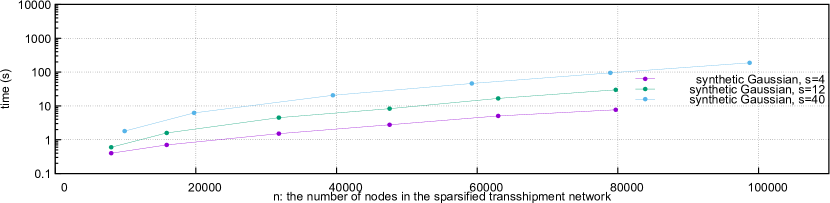
Figure 1: Plot of the empirical time (log scale) against the number of nodes $n$.

In Table 2, we present the total execution times for comparing four pairs of persistence diagrams: bh, AB, mri, rips from Table 5 in Section 4. The guaranteed relative error bound is given for each column. We achieve 50x, 15.6x, 56x and 4.3x speedup over hera with the bh, AB, mri and rips datasets at a guaranteed relative error of 0.5. When this error is 0.2, we achieve a speedup of 13.9x, 9.6x, 24.4x, and 2.2x respectively on the same datasets. We achieve a speedup of up to 3.90x and 5.67x on the AB dataset over the GPU-sinkhorn and the NtSmplx algorithm of POT respectively. Execution on rips is aborted early by POT. We also run PDoptFlow sequentially, doing the same total work as our parallel approach does. A slowdown of 1.1x-2.0x is obtained on bh at $\varepsilon=0.5$ and AB at $\varepsilon=0.2$ respectively compared to the parallel execution of PDoptFlow. This suggests most of PDoptFlow’s speedup comes from the approximation algorithm design irrespective of the parallelism. The Software from [22] is not in Table 2 since its theoretical relative error ($2\times$ (height of its quadtree)-1) [5, 22] is not comparable to values ($0.5$ and $0.2$) from Table 2. In fact, it has theoretical relative errors of $75,41,61,41$ for bh, AB, mri, rips respectively. flowtree [22] is much faster than PDoptFlow and is less accurate empirically. On these datasets, there is a 10.1x, 2.6x, 18.8x and 90.3x speedup against PDoptFlow($s=18$) at $\varepsilon=1.3$, for example.

NN PD Search for $W_{1}$ Time and Prediction Accuracy
	avg. time $\pm$ std. dev.	avg. recall@1 $\pm$ std. dev.
quadtree: ($\varepsilon=37.8\pm 0.5$)	0.46s $\pm$ 0.05s	2.2$\%$ $\pm$ 0.75$\%$
flowtree: ($\varepsilon=37.8\pm 0.5$)	4.88s $\pm$ 0.2s	44$\%$ $\pm$ 4.05$\%$
WCD	8.14s $\pm$ 2.0s	39.8$\%$ $\pm$ 2.71$\%$
RWMD	17.16s $\pm$ 0.97s	29.8$\%$ $\pm$ 5.74$\%$
PDoptFlow(s=1)	62.6s $\pm$ 3.38s	81$\%$ $\pm$ 5.2$\%$
PDoptFow(s=18): ($\varepsilon=1.4$)	371.2s $\pm$ 85s	95.4$\%$ $\pm$ 1.62$\%$
hera: ($\varepsilon=0.01$)	2014s $\pm$ 12.6s	100$\%$

Table 3: Total time for all $100$ NN queries and overall prediction accuracy over $5$ dataset splits of $50$/$50$ queries/search PDs; $\varepsilon$ is the theoretical relative error.

Table 3 shows the total time for $100$ NN queries amongst 100 PDs in the reddit dataset. The overall prediction accuracies using each of the algorithms are listed. See Section 4.1 for details on each of the approximation algorithms. Table 3 shows that the algorithms ordered from the fastest to the slowest on average on the reddit dataset are quadtree [5, 22], flowtree [5, 22], WCD [52], RWMD [52], PDoptFlow($s=1$), PDoptFlow($s=18$), and hera [50].

Table 3 also ranks the algorithms from the most accurate to the least accurate on average as hera, PDoptFlow($s=18$), PDoptFlow($s=1$), flowtree, WCD, RWMD, and quadtree. The average accuracy is obtained by $5$ runs of querying the reddit dataset $100$ times. PDoptFlow($s=18$) provides a guaranteed $2.3$-approximation which can even be used for ground truth distance since it computes 95% of the NNs accurately. Furthermore, it takes only one-fourth the time that Hera takes. Figure 2 shows the time-accuracy tradeoff of the seven algorithms in Table 3 on the reddit dataset.

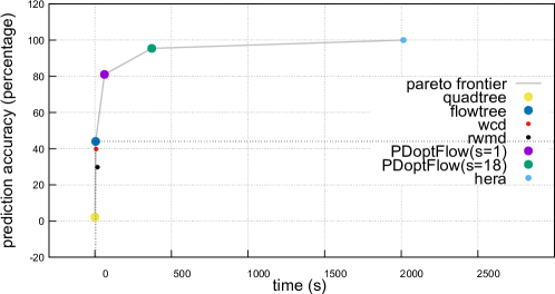
Figure 2: Pareto frontier of 7 algorithms showing the time and prediction accuracy tradeoff amongst the algorithms from Table 3 on the reddit dataset.

Figure 1 shows that our overall approach runs empirically in $O(s^{2}n^{1.5})$ time for small $s$ ($\leq 40)$. The empirical complexity improves with a smaller $s$. The datasets are given by synthetic 2D Gaussian point distributions on the plane acting as PDs. There are total of 10K, 20K, 40K, … 100K points in the synthetic PDs. We achieve up to 20% reduction in the total number of PD points by $\delta$-condensation. Section A.2.2 in the Appendix further explains the trend. This partly explains the speedups that Table 2 exhibits. For empirical relative errors, see Table 6 Section 4.

The rest of the paper explains our approach, implementation, and further experiments. Here is a table of the notations that follow.

Notations
Symbol	Meaning
$A,B$	input PDs
$\tilde{A},\tilde{B}$	multiset of points on $\mathbb{R}^{2}$ (nondiagonal points of $A$ and $B$)
$\Delta$	set of diagonal points
$\tilde{A}_{proj},\tilde{B}_{proj}$	multisets of projections of $\tilde{A},\tilde{B}$ to $\Delta$
$\hat{A},\hat{B}$	sets of points corresponding to $\tilde{A},\tilde{B}$
$\bar{a},\bar{b}$	virtual points that represent $\tilde{A}_{proj}$ and $\tilde{B}_{proj}$
$\hat{A}^{\delta}$, $\hat{B}^{\delta}$	$\delta$ condensation of $\hat{A}$ and $\hat{B}$
$\sigma,c,f$	supply, cost and flow functions of a transshipment network
$L,\delta$	a lower bound to the $W_{1}$-distance, additive error
WCD, RWMD	word centroid distance, relaxed word movers distance
$s,\varepsilon,n$	sparsification factor, theoretical relative error, and $|\tilde{A}\cup\tilde{B}|$
$G(A,B)$	bipartite transportation network on $\hat{A}\cup\{\bar{b}\}$ and $\hat{B}\cup\{\bar{a}\}$
$G_{\delta}$	$G(\hat{A}^{\delta}\cup\{\bar{b}\},\hat{B}^{\delta}\cup\{\bar{a}\})$
${\sf WS}_{s}(\hat{A}^{\delta}\cup\hat{B}^{\delta})$	s-WSPD on $(\hat{A}^{\delta}\cup\hat{B}^{\delta})$
${\sf WS}_{s}^{PD}(A^{\delta},B^{\delta})$	sparsified transshipment network induced by ${\sf WS}_{s}(\hat{A}^{\delta}\cup\hat{B}^{\delta})$
$W_{1}(A,B)$	ground truth $W_{1}$-distance

Table 4: Notations used in this paper.

2 1-Wasserstein Distance Problem

A persistence diagram is a multiset of points in the plane along with the points of infinite multiplicity on the diagonal line $\Delta$ (line with slope 1). The pairwise distances between diagonal points are assumed to be $0$. Each point $(b,d)$, $b\neq d$ in the multiset represents the birth and death time of a topological feature as computed by a persistence algorithm [35, 36]. Diagonal points are introduced to ascertain a stability [21, 25, 35] of PDs.

Given two PDs $A=\tilde{A}\cup\Delta$ and $B=\tilde{B}\cup\Delta$, $\tilde{A},\tilde{B}\subset\mathbb{R}^{2}\setminus\Delta$ let

$$W_{1}(A,B)=\adjustlimits{\inf}_{\Pi:A\rightarrow B}{\sum}_{x_{1}\in A}(\|x_{1}-\Pi(x_{1})\|_{2}),$$

where $\Pi$ is a bijection from $A$ to $B$. Notice that this formulation is slightly different from the ones in [32, 35] which takes the $l_{1}$ and $l_{\infty}$-norms respectively instead of the $l_{2}$-norm considered here. It is easy to check that this is equivalent to the following formulation:

$$\inf_{M\subset\tilde{A}\times\tilde{B}}{(\sum_{(x_{1},x_{2})\in M}(\|x_{1}-x_{2}\|_{2})+\sum_{x_{1}\notin\pi_{1}(M)}d_{\Delta}(x_{1})+\sum_{x_{2}\notin\pi_{2}(M)}d_{\Delta}(x_{2}))}$$

where $M$ is a partial one-to-one matching between $\tilde{A}$ and $\tilde{B}$; $\pi_{1}$, $\pi_{2}$ are the projections of the matching $M$ onto the first and second factors, respectively; $d_{\Delta}(x)$ is the $l_{2}$-distance of $x$ to its nearest point on the diagonal $\Delta$. The triangle inequality does not hold among the points on $\Delta$. In that sense, this $W_{1}$-distance differs from the classical Earth Mover’s Distance (EMD) [69] between point sets with the $l_{2}$ ground metric. Computing $W_{1}(A,B)$ (Problem 1) reduces to the problem of finding a minimizing partial matching $M\subset\tilde{A}\times\tilde{B}$.

Problem 1.

Given two PDs $A$ and $B$, Compute $W_{1}(A,B)$.

2.1 Matching to Min-Cost Flow

Let $\tilde{A}_{proj}$, $\tilde{B}_{proj}$ be the sets of points in $\Delta$ nearest (in $l_{2}$-distance) to $\tilde{A}$, $\tilde{B}$, respectively. Define the bipartite graph $\mathrm{Bi}(A,B)=(U_{1}\dot{\cup}U_{2},E)$ where $U_{1}:=\tilde{A}\cup\tilde{B}_{proj}$ and $U_{2}:=\tilde{B}\cup\tilde{A}_{proj}$. Define the point $p_{proj}$ to be the nearest point in $l_{2}$-distance to $p$ in $\Delta$ and let

$$E = (\tilde{A}\times\tilde{B})\cup\{(p,p_{proj})\}_{p\in\tilde{A}}\cup\{(q_{proj},q)\}_{q\in\tilde{B}}\cup(\tilde{A}_{proj}\times\tilde{B}_{proj}).$$

The edge $e=(p,q)\in E$ has weight (i) $0$ if $e\in\tilde{A}_{proj}\times\tilde{B}_{proj}$, (ii) weight $\|p-q\|_{2}$ if $p\in\tilde{A}$, $q\in\tilde{B}$, (iii) weight $d_{\Delta}(p)$ if $q=p_{proj}$, and (iv) weight $d_{\Delta}(q)$ if $p=q_{proj}$. Because of the edges with cost 0, minimizing the total weight of a perfect matching on $Bi(A,B)$ is equivalent to finding a minimizing partial matching $M\subset\tilde{A}\times\tilde{B}$ and thus computing $W_{1}(A,B)$ in turn.

Let $G=(V,E,c,\sigma)$ be a transshipment network made up of nodes and directed edges called arcs where we have a supply function $\sigma:V(G)\rightarrow\mathbb{Z}$, a cost function $c:V(G)\times V(G)\rightarrow\mathbb{R}^{+}$, and a flow function $f:V(G)\times V(G)\rightarrow\mathbb{Z}$. Define the uncapacitated min-cost flow on $G$ as:

$$\min_{\Sigma_{u}f(u,v)=|\sigma(v)|,\Sigma_{v}f(u,v)=|\sigma(u)|,f(u,v)\geq 0}c(u,v)\cdot f(u,v),\text{where }(u,v)\in E(G).$$

Now we describe a construction of the bipartite transshipment network $G(A,B)$ for two PDs $A$ and $B$. Intuitively, $G(A,B)$ is $Bi(A,B)$ with a set instead of multiset representation for the nodes. Let $\pi_{A}$ and $\pi_{B}$ denote the mapping of the points in $\tilde{A}\cup\tilde{B}_{proj}$ and $\tilde{B}\cup\tilde{A}_{proj}$ respectively to the nodes in the graph $G(A,B)$. All points with distance $0$ are mapped to the same node by $\pi_{A}$ and $\pi_{B}$. Since the diagonal points $\tilde{A}_{proj}$ and $\tilde{B}_{proj}$ are assumed to have distance zero, all points in $\tilde{A}_{proj}$ map to a single node, say $\bar{a}=\pi_{A}(\tilde{A}_{proj})$. Similarly, all points in $\tilde{B}_{proj}$ map to a single node, say $\bar{b}=\pi_{B}(\tilde{B}_{proj})$ (See Figure 3). We call this $0$-condensation because it does not perturb the non-diagonal PD points. All arcs to or from $\bar{a}$ or $\bar{b}$ form diagonal arcs, which are used in our main algorithm.

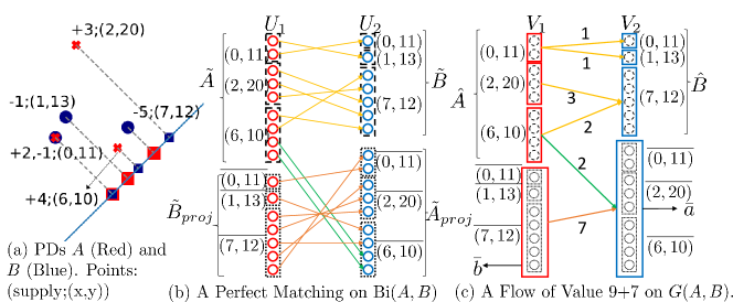
Figure 3: (a) $-5;(7,12)$ means a supply of $-5$ units at point $(7,12)$. (b) $\mathrm{Bi}(A,B)$ with the nodes denoted by solid circles. (c) $G(A,B)$, nodes are the solid outer boxes. Supplies in $G(A,B)$ are set by the number of circles inside each box. In (b) and (c), barred-points e.g. $\overline{(7,12)}$ are projections to the diagonal.

Let $\hat{A}$ and $\hat{B}$ denote the set of nodes corresponding to the non-diagonal points, that is, $\hat{A}=\pi_{A}(\tilde{A})$, $\hat{B}=\pi_{B}(\tilde{B})$. The nodes of $G(A,B)$ are $(\hat{A}\cup\{\bar{b}\})\dot{\cup}(\hat{B}\cup\{\bar{a}\})$. The vertices of the transshipment network $G(A,B)$ are assigned supplies $\sigma(u)=|\pi_{A}^{-1}(u)|$ for $u\in U_{1}$ and $\sigma(v)=-|\pi_{B}^{-1}(v)|$ for $v\in U_{2}$. Intuitively, negative supply at a node means that there is a demand for a net flow at that node, which corresponds to a point in $B$. The intuition for positive supply is analogous.

Proposition 2.1.

There is a perfect matching on $\mathrm{Bi}(A,B)$ with $|\tilde{A}|=n_{1}$ and $|\tilde{B}|=n_{2}$ iff there is a feasible flow of value $n_{1}+n_{2}$ in $G(A,B)$.

Proof.

$\Rightarrow$ Any perfect matching $\mu$ on $\mathrm{Bi}(A,B)$ can be converted to a feasible flow on $G(A,B)$ by assigning a flow between $u\in U_{1}$ and $v\in U_{2}$ equal to the number of pairs $(p,\mu(p))$ with $p\in\pi^{-1}(u)$ and $\mu(p)\in\pi^{-1}(v)$. The supplies on $G(A,B)$ are met because of the way $G(A,B)$ is constructed. The value of the flow for the conversion is $n_{1}$+$n_{2}$ since there were that many pairings in the perfect matching.

$\Leftarrow$ Given a feasible flow of value $n_{1}+n_{2}$ on $G(A,B)$, we obtain a matching on $\mathrm{Bi}(A,B)$ by observing that we can decompose any feasible flow on arc $(u,v)\in\hat{A}\cup\{\bar{b}\}\times\hat{B}\cup\{\bar{a}\}$, into unit flows from $\pi^{-1}_{A}(u)$ to $\pi^{-1}_{B}(v)$ with no pair repeating any point from other pairs. Each unit flow corresponds to a pair in the matching. Since the flow has $n_{1}+n_{2}$ flow value, there must be the $n_{1}+n_{2}$ pairings in the matching, making it perfect. ∎

Problem 1 reduces to a min-cost flow problem on $G(A,B)$ by Proposition 2.1. A proof based on linear algebra can be found in [53].

3 Approximating 1-Wasserstein Distance

In this section we design a $(1+O(\varepsilon))$-approximation algorithm for Problem 1 that first sparsifies the bipartite graph $G(A,B)$ with an algorithm incurring a cost of $\tilde{O}_{\varepsilon}(n)$, where $\tilde{O}_{\varepsilon}$ hides a polylog dependence on $n$ and a polynomial dependence on $\frac{1}{\varepsilon}$. Due to the node and edge sparsification, we must then use the min-cost flow formulation of Section 2 instead of a bi-partite matching for computing an approximation to the $W_{1}$-distance. We use the network simplex algorithm to solve the min-cost flow problem because it suits our purpose aptly though theoretically speaking any min-cost flow algorithm can be used.

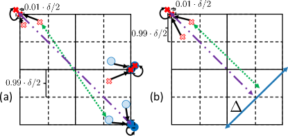
Figure 4: $\delta$-condensation for (a) matched and (b) unmatched points. Points snapped to their nearest $0.99\delta$-grid point. Points are then perturbed in a $0.01(\frac{\delta}{2})$ neighborhood. Green dotted pairwise distances change to new purple dotted and dashed pairwise distances.

3.1 Condensation (Node Sparsification)

As the size of the PD increases, many of its points cluster together since filtration values often become close. This is because the filtration values may come from, for example, scale-free [6] social network data, that is, graphs with power law degree distributions, or voxelized data given as finitely many grid values. See Section A.1.3 for a discussion on the clustering of PD points and how do they arise from scale-free graphs and voxel data. Figure 6 shows such evidences for voxelized data. We draw upon a common technique for rasterizing the plane by snapping points to an evenly spaced grid to decrease the number of points. As discussed in Section A.2, it is known that the network simplex algorithm performs better on a transshipment network with many different arc lengths than the one with many arcs having the same length. To avoid the symmetry induced by the lattice, we perturb randomly the combined points. For a $\delta>0$ and a fraction $k\geq 0.5$ (say $k=0.99$), we snap nondiagonal points to a $k\delta\cdot\mathbb{Z}\times k\delta\cdot\mathbb{Z}$ lattice (grid). Let $\pi_{\delta}:\hat{A}\cup\hat{B}\rightarrow(k\delta\cdot\mathbb{Z})\times(k\delta\cdot\mathbb{Z}$) define this snapping of a point to its nearest $\delta$-lattice point where $\pi_{\delta}((x,y))=(k\delta\cdot round(\frac{x}{k\delta}),k\delta\cdot round(\frac{y}{k\delta}))$. We follow the snapping by $\pi_{\delta}$ with a random shift of each condensed point by at most $\frac{1-k}{2}\cdot\delta$ in any of the $\pm x$ or $\pm y$ directions; see Figure 4. We call the entire procedure as ”$\delta$-condensation” or ”$\delta$-snapping”. The aggregate of the points snapped to a grid point is accounted for by a supply value assigned to it; see Algorithm 2.

Proposition 3.1.

Let $A$ and $B$ be two PDs and $\varepsilon>0$. For $\delta:=\frac{2\varepsilon L}{\sqrt{2}(|\tilde{A}|+|\tilde{B}|)}$ where $L\leq W_{1}(A,B)$, let the snapping by $\pi_{\delta}$ followed by a $\delta\cdot(1-k)/2$ random shift on $A$ and $B$ produce $A^{\delta}$ and $B^{\delta}$ respectively. Then, $(1-\varepsilon)W_{1}(A,B)\leq W_{1}(A^{\delta},B^{\delta})\leq(1+\varepsilon)W_{1}(A,B)$.

Proof.

After applying $\pi_{\delta}$, each point moves in a $\frac{\sqrt{2}\delta}{2}$ neighborhood. Thus for any pair of nondiagonal points $p\in\tilde{A}$ and $q\in\tilde{B}$, the $l_{2}$-distance between the two points shrinks/grows at most by $\frac{2\sqrt{2}k\delta}{2}$ units. A $\frac{(1-k)\delta}{2}$-perturbation contributes to an error of $\frac{2\sqrt{2}(1-k)\delta}{2}$ units for the $l_{2}$-distance between $p$ and $q$. Thus, for a pair of nondiagonal points the additive error incurred is $\sqrt{2}\delta$ units. Furthermore, for any nondiagonal point in either diagram, its distance to $\Delta$ can shrink/grow by at most $\frac{\sqrt{2}k\delta}{2}+\frac{\sqrt{2}(1-k)\delta}{2}=\frac{\sqrt{2}\delta}{2}$ units.

Let $m_{1}$ be the number of pairs of matched nondiagonal points and $m_{2}$ be the number of unmatched nondiagonal points. Let the $\delta$-condensation of A and B be $A^{\delta},B^{\delta}$ and let $\delta^{\prime}=\sqrt{2}(m_{1}+\frac{m_{2}}{2})\delta$. To reach the conclusion of the proposition, we want $\delta$ to induce a relative error of $\varepsilon$ for $W_{1}(A^{\delta},B^{\delta})$ with respect to $W_{1}(A,B)$ satisfying the following inequalities:

$$(1-\varepsilon)W_{1}(A,B)\leq W_{1}(A,B)-\delta^{\prime}\leq W_{1}(A^{\delta},B^{\delta})\leq W_{1}(A,B)+\delta^{\prime}\leq(1+\varepsilon)W_{1}(A,B).$$

Observe that $m_{1}+\frac{m_{2}}{2}=\frac{(|\tilde{A}|+|\tilde{B}|)}{2}$. Also, we have that $L\leq W_{1}(A,B)$. These together constrain $\delta$ to satisfy $\sqrt{2}(m_{1}+\frac{m_{2}}{2})\delta=\sqrt{2}\frac{(|\tilde{A}|+|\tilde{B}|)}{2}\delta\leq\varepsilon L\leq\varepsilon W_{1}(A,B)$, which gives the desired value of $\delta$ as stated. ∎

A lower bound $L$ from Proposition 3.1 is needed in order to convert the additive error of $\delta$ to a multiplicative error of $1\pm\varepsilon$. To find the lower bound $L$, we use the Relaxed Word Mover’s distance (RWMD) [52] that gives a lower bound for the min-cost flow of $G(A,B)$, hence for $W_{1}(A,B)$. There are many lower bounds that can be used such as those from [4, 52]. However, we find RWMD to be the most effective in terms of computational time and approximation in general.

Recall that RWMD is a relaxation of one of the two constraints of the min-cost flow problem. If we ”relax” or remove the constraint $\sum_{v}f(u,v)=|\sigma(u)|,u\in\hat{B}\cup\{\bar{a}\}$ from the min-cost flow formulation, we obtain the following feasible flow to the min-cost flow with one of its constraints removed

$$f^{low,A}(u,v)=\left\{\begin{array}[]{ll}|\sigma(u)|&\quad\text{if }v=\mathrm{argmin}_{v^{\prime}}\,c(u,v^{\prime})\\ 0&\quad\text{otherwise}\end{array}\right.$$

and evaluate $L_{A}:=\sum_{u,v}c(u,v)\cdot f^{low,A}(u,v)$. Since $W_{1}(A,B)$ is a feasible solution to the relaxed min-cost flow problem, $L_{A}\leq W_{1}(A,B)$. Relaxing the constraint $\sum_{u}f(u,v)=|\sigma(v)|,v\in\hat{A}\cup\{\bar{b}\}$, we can define $f^{low,B}(u,v)$ and $L_{B}$ similarly.

Our simple parallel algorithm involves computing $L:=\max(L_{A},L_{B})$, the RWMD, by exploiting the geometry of the plane via a kd-tree to perform fast parallel nearest neighbor queries. For $L_{A}$, we first construct a kd-tree for $\hat{B}$ viewed as points in the plane, then proceed to search in parallel for every $u\in\hat{A}$, its nearest $l_{2}$-neighbor $v^{*}$ in $\hat{B}$ while writing the quantity $c(u,v^{*})\cdot f^{low,A}(u,v^{*})$ to separate memory addresses. Noticing that the closest point to $\bar{b}$, is $\bar{a}$ at cost $0$, it suffices to consider the points $\hat{A}$ to compute $L_{A}$. We then apply a sum-reduction to the array of products, taking $O(\log n)$ depth [11]. We apply a similar procedure for $L_{B}$. See Algorithm 1.

1:build kd-tree on $\hat{B}$ using Euclidean distance on $\mathbb{R}^{2}$

2:compute $v^{*}=\mathrm{argmin}_{v\in\hat{B}}c(u,v)$ by NN search on $\hat{B}$ and store $f^{low,A}(u,v^{*})$ for each $u\in\hat{A}$ in parallel

3:$L_{A}\leftarrow$ compute sum-reduction of line $2$

4:$L_{B}\leftarrow$ compute lines 1-3 with $\hat{A}$ and $\hat{B}$ swapped return $\max(L_{A},L_{B})$

Algorithm 1 RWMD($\hat{A},\hat{B}$, $c$)

Since the kd-tree queries each takes $O(\sqrt{n})$ sequential time, we obtain an algorithm with $O(n)$ processors requiring $O(\sqrt{n}+\log n)=O(\sqrt{n})$ depth and $O(n\sqrt{n})$ work.

1:PDs $A,B$, $s>0$

2:$(\hat{A},\bar{b},\sigma_{\hat{A}},\hat{B},\bar{a},\sigma_{\hat{B}})\leftarrow$ 0-condense$(A,B)$

3:$L\leftarrow RWMD(\hat{A},\hat{B},c)$ $\triangleright$ $c(\cdot,\cdot)$ from Section 2

4:$\varepsilon\leftarrow\frac{8}{s-4}$ if $s\geq 12$ else $\varepsilon\leftarrow 1$; $\delta\leftarrow\frac{2\varepsilon L}{\sqrt{2}(|\tilde{A}|+|\tilde{B}|)}$

5:$(\hat{A}^{\delta}$, $\hat{B}^{\delta})$ $\leftarrow$ $(\pi_{\delta}(\hat{A}),\pi_{\delta}(\hat{B}))$ $\triangleright$ snap points of $\hat{A}$, $\hat{B}$ to a common $0.99\delta$-lattice

6:$\sigma_{\hat{A}^{\delta}\cup\hat{B}^{\delta}\cup\{\bar{a}\}\cup\{\bar{b}\}}$ $\leftarrow$$\begin{cases}\sum_{u\in\pi^{-1}_{\delta}(v)}\sigma(u)&v\in\hat{A}^{\delta}\cup\hat{B}^{\delta}\\ \sigma(v)&v=\{\bar{a}\}\cup\{\bar{b}\}\end{cases}$

7:perturb $\hat{A}^{\delta}\cup\hat{B}^{\delta}$ in a $\frac{0.01}{2}\delta$-radius square return $(\hat{A}^{\delta}\cup\hat{B}^{\delta},\sigma_{\hat{A}^{\delta}\cup\hat{B}^{\delta}\cup\{\bar{a}\}\cup\{\bar{b}\}})$

Algorithm 2 $\delta$-condensation

The algorithm for $\delta$-condensation is given in Algorithm 2. We first gather all the points based on their $x$ and $y$ coordinates called a $0$-condensation; see Section 2. Then, we compute the RWMD in order to compute $\delta$. This $\delta$ depends on an intermediate relative error of $\varepsilon$ for $\delta$-condensation, which depends on the input $s$. The quantity $\varepsilon$ is chosen to be less than $1$. In particular, we set $\varepsilon\leftarrow\frac{8}{s-4}$ if $s\geq 12$ and $\varepsilon\leftarrow 1$ otherwise; see line 3 in Algorithm 2. Finally, we snap the points of $\hat{A}$ and $\hat{B}$ to the $\delta$-grid and then perturb the condensed points in a small neighborhood. The resulting sets of points are denoted $\hat{A}^{\delta}$ and $\hat{B}^{\delta}$. For each condensed point, we aggregate the supplies of points that are snapped to it. The aggregated supply function is denoted $\sigma_{\hat{A}^{\delta}\cup\hat{B}^{\delta}\cup\{\bar{a}\}\cup\{\bar{b}\}}$. The bipartite transshipment network that could be constructed by placing arcs between all nodes from $A^{\delta}:=\hat{A}^{\delta}\cup\{\bar{b}\}$ to $B^{\delta}:=\hat{B}^{\delta}\cup\{\bar{a}\}$ is denoted as $G_{\delta}$:=$G(A^{\delta},B^{\delta})$. The cost $c_{\delta}$ is defined on arcs of $G(A^{\delta},B^{\delta})$ as $c_{\delta}(u,v)=\|u-v\|_{2}$ for $u\in\hat{A}^{\delta}$ and $v\in\hat{B}^{\delta}$. The costs $c_{\delta}(u,\bar{a})$ and $c_{\delta}(\bar{b},v)$ are defined by the $l_{2}$-distances of $u$ and $v$ to $\Delta$ as in Section 2.1. Furthermore, the supply on all points is defined by $\sigma_{A^{\delta}\cup B^{\delta}}$. Only the nodes and supplies of this network are constructed.

3.2 Well Separated Pair Decomposition(Arc Sparsification)

The node sparsification of $G(A,B)$ gives $G_{\delta}$ whose arcs are further sparsified. Using Theorem $1$ in [14], we bring the quadratic number of arcs down to a linear number by constructing a geometric $(1+\varepsilon)$-spanner on the point set $\hat{A}^{\delta}\cup\hat{B}^{\delta}$. For a point set $P\subset\mathbb{R}^{2}$, let its complete distance graph be defined with the points in $P$ as nodes where every pair $p,q\in P$, $p\not=q$, is joined by an edge with weight equal to $\|p-q\|_{2}$. Define a geometric $t$-spanner $S(P)$ as a subgraph of the complete distance graph of $P$ where for any $p,q\in P,p\neq q$, the shortest path distance $d_{SP}(p,q)$ between $p$ and $q$ in $S(P)$ satisfies the condition $d_{SP}(p,q)\leq t\cdot\|p-q\|_{2}$.

We compute a spanner using the well separated decomposition $s$-WSPD [20, 45]. Notice that there are many other possible spanner constructions such as $\theta$-graphs [24, 49] and others, e.g. [44, 55]. However, experimentally we find that WSPD is effective in practice, and becomes especially effective when $s$ is small. The $\theta$-graphs, for example, can be an order of magnitude slower to compute as implemented in the CGAL software [39]. This is theoretically justified by the $O(\log n)$ factor in the $O(n\log n)$ construction time of $\theta$-graphs when $n>1024$. An $s$-WSPD is a well known geometric construction that approximates the pairwise distances between points by pairs of ”$s$-well-separated” point subsets. Two point subsets $U$ and $V$ are $s$-well separated in $l_{2}$-norm if there exist two $l_{2}$ balls of radius $d$ containing $U$ and $V$ that have distance at least $d\cdot s$. An $s$-WSPD of a point set $P\subset\mathbb{R}^{2}$ is a collection of pairs of $s$-well separated subsets of $P$ so that for every pair of points $p,q\in P$, $p\neq q$, there exists a unique pair of subsets $U,V$ in the $s$-WSPD with $U\ni p$ and $V\ni q$. Each subset in an $s$-WSPD is represented by an arbitrary but fixed point in the subset. We can construct a digraph ${\sf WS}_{s}(P)$ from the $s$-WSPD on $P$ by taking the point representatives as nodes and placing biarcs between any two nodes $u,v$, that is, creating both arcs $(u,v)$ and $(v,u)$. It is known [20, 45] that ${\sf WS}_{s}(P)$, viewed as an undirected graph, is a geometric t-spanner for $t=(s+4)/(s-4)$. Putting $t=(1+\varepsilon)$, this gives $s=4+\frac{8}{\varepsilon}$. It was recently shown in [30] that by taking leftmost points as representatives in the well separated subsets, one can improve $t$ to $1+\frac{4}{s}+\frac{4}{s-2}$. Furthermore, it is also known that ${\sf WS}_{s}(P)$ has $O(s^{2}n)$ number of arcs where $n=|P|$.

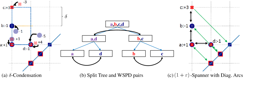
Figure 5: Illustration of Algorithm 3: (a) $\delta$-condensation for the example in Figure 3 with the split tree construction on $\hat{A}^{\delta}\cup\hat{B}^{\delta}$; (b) WSPD pairs (black biarcs) on the split tree from (a); and (c) the induced transshipment network from the WSPD with the green diagonal arcs included.

Now we describe how we compute an arc sparsification of $G_{\delta}$. To save notations, we assume the points of $\hat{A}^{\delta}$ and $\hat{B}^{\delta}$, the $\delta$-condensation of $\hat{A}$ and $\hat{B}$ respectively, to be nodes also. We compute a $(1+\varepsilon)$-spanner ${\sf WS}_{s}(\hat{A}^{\delta}\cup\hat{B}^{\delta})$ via an $s$-WSPD on the points $\hat{A}^{\delta}\cup\hat{B}^{\delta}$. Notice that this digraph has all nodes of $G_{\delta}$ except the two diagonal nodes $\bar{a}$ and $\bar{b}$ which we add to it with all the original arcs from $\bar{a}$ and to $\bar{b}$ having the cost same as in $G_{\delta}$. Now we assign supplies to nodes in ${\sf WS}_{s}(\hat{A}^{\delta}\cup\hat{B}^{\delta})$ as in $G_{\delta}$. There is a caveat here. It may happen that points from $\hat{A}^{\delta}$ and $\hat{B}^{\delta}$ overlap. Two such overlapped points from two sets are represented with a single point having the supply equal to the supplies of the overlapped points added together. Let ${\sf WS}_{s}^{PD}(A^{\delta},B^{\delta})$ denote this sparsified transshipment network. Adapting an argument in [14] to our case, we have:

Theorem 3.2.

Let $f^{*}$ and $\bar{f}^{*}$ be the min-cost flow values in $G_{\delta}$ and ${\sf WS}_{s}^{PD}(A^{\delta},B^{\delta})$ respectively where $s$ satisfies $\varepsilon=\frac{4}{s}+\frac{4}{s-2}$ for some $\varepsilon>0$. Then $f^{*}$ and $\bar{f}^{*}$ satisfy $f^{*}\leq\bar{f}^{*}\leq(1+\varepsilon)f^{*}$.

Proof.

First, notice that the nodes of ${\sf WS}_{s}^{PD}(A^{\delta},B^{\delta})$ are exactly the same as in $G(A^{\delta},B^{\delta})=(A^{\delta}\dot{\cup}B^{\delta},A^{\delta}\times B^{\delta},c_{\delta},\sigma_{A^{\delta}\cup B^{\delta}})$ except the overlapped nodes. We can decompose the overlapped nodes back to their original versions in $\hat{A}^{\delta}$ and $\hat{B}^{\delta}$ with biarcs of $0$-distance between them. This will also restore the supplies at each node. This does not affect $\bar{f}^{*}$. Let the cost $c_{\delta}(u,v)$ in ${\sf WS}_{s}^{PD}(A^{\delta},B^{\delta})$ be the $l_{2}$-distance between corresponding points of $u$ and $v$ for $u,v\in\hat{A}^{\delta}\sqcup\hat{B}^{\delta}$ (all non-diagonal points pairs). Furthermore, let $c_{\delta}(\bar{b},v),v\in\hat{B}^{\delta}$ and $c_{\delta}(u,\bar{a}),u\in\hat{A}^{\delta}$ have cost exactly as in $G(A^{\delta},B^{\delta})$. Recall that in ${\sf WS}_{s}^{PD}(A^{\delta},B^{\delta})$ there is no arc between $\hat{A}^{\delta}$ and $\bar{b}$ nor between $\hat{B}^{\delta}$ and $\bar{a}$. Treating the costs on the arcs as weights, let the shortest path distance between $u$ and $v$ be $d_{SP}^{{\sf WS}}(u,v)$ on ${\sf WS}_{s}^{PD}(A^{\delta},B^{\delta})$. We already have a $(1+\varepsilon)$-spanner ${\sf WS}_{s}(\hat{A}^{\delta}\cup\hat{B}^{\delta})$, and adding the nodes $\bar{a}$ and $\bar{b}$ with the diagonal arcs to form ${\sf WS}_{s}^{PD}(A^{\delta},B^{\delta})$ still preserves the spanner property, namely

$$d_{SP}(\bar{b},v)=c_{\delta}(\bar{b},v)\leq(1+\varepsilon)c_{\delta}(\bar{b},v)\text{ for }v\in B^{\delta}$$

and

$$d_{SP}(u,\bar{a})=c_{\delta}(u,\bar{a})\leq(1+\varepsilon)c_{\delta}(u,\bar{a})\text{ for }u\in A^{\delta}.$$

Let $f$ and $\bar{f}$ denote the respective flows for $f^{*}$ and $\bar{f}^{*}$. We can now prove the conclusion of the theorem.

$f^{*}\leq\bar{f}^{*}$: $\bar{f}$ can be decomposed into flows along paths from nodes in $A^{\delta}$ to nodes in $B^{\delta}$. One can get a flow $\hat{f}$ on $G(A^{\delta},B^{\delta})$ from $\bar{f}$ by considering a flow on every bipartite arc $(u,v)$ in $G(A^{\delta},B^{\delta})$ which equals the path decomposition flow from $u$ to $v$ in ${\sf WS}^{PD}_{s}(A^{\delta},B^{\delta})$. We have

$$f^{*}=\sum_{(u,v)\in G(A^{\delta},B^{\delta})}c_{\delta}(u,v)\cdot f_{uv}\leq\sum_{(u,v)\in G(A^{\delta},B^{\delta})}c_{\delta}(u,v)\cdot\hat{f}_{uv}\leq\sum_{(u,v)\in A^{\delta}\times B^{\delta}}d_{P}^{{\sf WS}}(u,v)\cdot\hat{f}_{uv}=\bar{f}^{*},$$

where $d_{P}^{{\sf WS}}(u,v)$ is the path distance on ${\sf WS}_{s}^{PD}(A^{\delta},B^{\delta})$ as determined by the flow decomposition. The leftmost inequality follows since $\hat{f}$ is a feasible flow on $G(A^{\delta},B^{\delta})$ and the rightmost inequality follows since any path length between two nodes $u$ and $v$ is bounded from below by the direct distance $c_{\delta}(u,v)$ between the points they represent. The last equality follows by the flow decomposition.

$\bar{f}^{*}\leq(1+\varepsilon)f^{*}$:

$$\bar{f}^{*}\leq\sum_{(u,v)\in A^{\delta}\times B^{\delta}}d_{SP}^{{\sf WS}}(u,v)\cdot f_{uv}\leq\sum_{(u,v)\in G(A^{\delta},B^{\delta})}(1+\varepsilon)c_{\delta}(u,v)\cdot f_{uv}=(1+\varepsilon)f^{*}.$$

The leftmost inequality follows since the flow $f$ of $G(A^{\delta},B^{\delta})$ sent across shortest paths forms a feasible flow on ${\sf WS}_{s}^{PD}(A^{\delta},B^{\delta})$. To check this, notice that the supplies are all satisfied for every node in ${\sf WS}_{s}^{PD}(A^{\delta},B^{\delta})$. Any intermediate node of a shortest path between $u\in A^{\delta}$ and $v\in B^{\delta}$ gets a net change of 0 supply. The rightmost inequality follows because ${\sf WS}_{s}^{PD}(A^{\delta},B^{\delta})$ still satisfies the $(1+\varepsilon)$-spanner property as mentioned above. ∎

$s$-WSPD Construction: In order to construct an $s$-WSPD, a hierarchical decomposition such as a split tree or quad tree is constructed. We build a split tree due to its simplicity and high efficiency. A split tree can be computed sequentially with any of the standard algorithms in [16, 20, 45] that runs in $O(n\log n)$ time. It is not a bottleneck in practice. This is because there is only $O(n)$ writing to memory for constructing the tree. A simple construction of the split tree $T$ starts with a bounding box containing the input point set followed by a recursive division that splits a box into two halves by dividing the longest edge of the box in the middle. The split tree construction for a given box stops its recursion when it has one point.

Sequential construction of a WSPD involves collecting all well separated pairs of nodes which represent point subsets from the split tree $T$. This is done by searching for descendant node pairs from each interior node $w$ in $T$. For each pair of descendant nodes $u$ and $v$ reached from $w$, the procedure recursively continues the search on both children of the node amongst $u$ and $v$ that has the larger diameter for its bounding box. When the points corresponding to a pair of nodes $u,v$ become well separated, we collect $(u,v)$ in the WSPD and stop recursion.

The construction of WSPD is the primary bottleneck before the min-cost flow computation. The sequential computation incurs high data movement and also a large hidden constant factor in the complexity. To overcome these difficulties, we compute the WSPD in parallel while still preserving locality of reference, only using $n-1$ threads, and $O(n)$ auxiliary memory. We propose a simple approach on multicore that avoids linked lists or arbitrary pointers as in [15, 16]. A unique thread is assigned to each internal node $w$ in the split tree $T$. Then, we write a prefix sum [54] of the counts of well separated pairs found by each thread. Following this, each thread on $w\in T$ re-searches for well separated pairs and independently writes out its well separated descendant nodes in its memory range as determined by the prefix sum. Recursive calls on split tree node pairs can also be run in parallel as in [77]; doing so requires an unbounded data structure to store the pairs found by each thread such as a 2-layer tree with blocks at its leaves. Such a parallel algorithm can have worst-case depth of $O(\text{polylog}(s^{2}n))$ and work complexity of $O(s^{2}n)$. In practice, we can gain speedup in our simplified implementation, which does not issue recursive calls at interior nodes and thus has $O(s^{2}n)$ depth. This is because significant work can arise at internal nodes near the leaves. For an illustration of the implementation, see Appendix.

3.3 Min-cost Flow by Network Simplex

Having constructed a sparsified transshipment network, we solve the min-cost flow problem on this network with an efficient implementation of the network simplex (NtSmplx) algorithm.

The NtSmplx algorithm is a graph theoretic version of the simplex algorithm used for linear programming. It involves the search for basic feasible min-cost flow solutions. This is done by successively applying pivoting operations to improve the objective function. A pivot involves an interchange of arcs for a spanning tree on the transshipment network. As observed in [51], we also find that the pivot searching phase for the incoming arc during pivoting dominates the runtime of NtSmplx. In particular, it is vital to have an efficient pivot searching algorithm: to quickly find a high quality entering arc that lessens the number of subsequent pivots. Authors in [43] propose an interpolation between Dantzig’s greedy pivot rule [28] and Bland’s pivot rule [10] by the block search pivot (BSP) algorithm. This implementation for NtSmplx is adopted in [33]. It is found empirically in [51] that the BSP algorithm is very efficient, simple, and results in a low number of degenerate pivots in practice. We use the BSP algorithm in our implementation because of these reasons.

Notice that if dynamic trees [74] are used, the complexity of a pivot search can be brought down to $O(\log n)$ and thus NtSmplx can run in time $\tilde{O}(s^{2}n^{2})$ [1, 42] on our WSPD spanner.

BSP sacrifices theoretical guarantees for simplicity and efficiency in practice. During computation, degenerate pivots, or pivots that do not make progress in the objective function may appear. There is the possibility of stalling or repeatedly performing degenerate pivots for exponentially many iterations. As Section A.2 in Appendix illustrates, stalling drives the execution to a point where no progress is made. However, our experiments suggest that, before stalling, BSP usually arrives at a very reasonable feasible solution.

We observe that performance of NtSmplx depends heavily on the sparsity of our network. Since a pivot involves forming a cycle with an entering arc and a spanning tree in the network, if the graph is sparse there are few possibilities for this entering arc.

3.4 Approximation Algorithm

The approximation algorithm is given in Algorithm 3, which proceeds as follows. Given input PDs $A$ and $B$ and the parameter $s>2$, first we set $\varepsilon=\frac{8}{s-4}$. We compute a $\delta$ according to Proposition 3.1 using this $\varepsilon$ for $s\geq 12$ and setting $\varepsilon=1$ for $2<s<12$. Then, we perform a $\delta$-condensation and compute an $s$-WSPD via a split tree construction on $\hat{A}^{\delta}\cup\hat{B}^{\delta}$.

We then compute ${\sf WS}_{s}(\hat{A}^{\delta}\cup\hat{B}^{\delta})$ from the $s$-WSPD. It is a $(1+\varepsilon^{\prime})$-spanner for $s>2$ where $\varepsilon^{\prime}=\frac{4}{s}+\frac{4}{s-2}$. Diagonal nodes along with their arcs are added to this graph as determined by $G_{\delta}$. This means that we add the nodes $\bar{a}$ and $\bar{b}$ and all arcs from $\hat{A}^{\delta}$ to $\bar{b}$ and $\bar{a}$ to $\hat{B}^{\delta}$. This produces ${\sf WS}_{s}^{PD}(A^{\delta},B^{\delta})$. Figure 5 shows our construction. The network simplex algorithm is applied to the sparse network ${\sf WS}_{s}^{PD}(A^{\delta},B^{\delta})$ to get a distance that approximates the min-cost flow value on $G_{\delta}$ within a factor of $(1+\varepsilon^{\prime})$ between inputs $A^{\delta}$ and $B^{\delta}$. The algorithm still runs for $s>0$ instead of $s>2$ since we can still construct a valid transshipment network for optimization. However, there are no guarantees if $s\leq 2$. Nonetheless, empirical error is found to be low and the computation turns out very efficient; see Section 4.

1:PDs: $A,B$, $s>2$ the sparsity parameter, $\varepsilon=\frac{8}{s-4}$ for $s\geq 12$ and $\varepsilon=1+\frac{8}{s}+\frac{8}{s-2}$ for $2<s<12$

2:a $(1+O(\varepsilon))$-approximation to $W_{1}$-distance

3:$(\boldsymbol{P}$,$\sigma_{\boldsymbol{P}})\leftarrow$ $\delta$-condensation$(A,B,s)$ $\triangleright$ $\boldsymbol{P}=\hat{A}^{\delta}\cup\hat{B}^{\delta}$

4:$\boldsymbol{T}\leftarrow$ form-splittree($\boldsymbol{P}$)

5:nondiag-arcs $\leftarrow$ form-WSPD$(\boldsymbol{T},s)$ $\triangleright$ $1+\varepsilon$-spanner

6:diag-arcs $\leftarrow$ form-diag-arcs$(\boldsymbol{P})$ $\triangleright$ diagonal arcs constructed as in Section 2.1

7:$\boldsymbol{G}\leftarrow(\boldsymbol{P}$, nondiag-arcs $\cup$ diag-arcs, $\sigma_{\boldsymbol{P}}$, $c:=$dists(nondiag-arcs $\cup$ diag-arcs)) $\triangleright$ Defn. 2.1 return min-cost flow$(\boldsymbol{G})$

Algorithm 3 Approximate $W_{1}$-Distance Algorithm

The time complexity of the algorithm is dominated by the computation of the min-cost flow routine. Thus, all the steps of our algorithm are designed to improve the efficiency of the NtSmplx algorithm. Replacing NtSmplx with the algorithm in [12], a complexity of $\tilde{O}(ns^{2}+n^{1.5})$ can be achieved. However, NtSmplx is simpler, more memory efficient, has a reasonable complexity of $\tilde{O}(s^{2}n^{2})$ [74], and is very efficient in practice; see Figure 1 and Figure 12 in Appendix.

3.5 Theoretical Bounds

By Theorem 3.2, the spanner achieves a $(1+\frac{4}{s}+\frac{4}{s-2})$-approximation to the min-cost flow value on the $\delta$-condensed graph. A $\delta$-condensation results in an approximation of the $W_{1}$-distance with a factor of $(1\pm(\frac{8}{s-4}))$ for $s\geq 12$ and $2$ for $2<s<12$. The factor $2$ for the range $2<s<12$ is obtained by putting $s=12$ in $\frac{8}{s-4}$ because $s\leq 12$ and we need $\frac{8}{s-4}>0$. The node and arc sparsifications together guarantee an approximation factor of $((1+\frac{4}{s}+\frac{4}{s-2})(1\pm(\frac{8}{s-4})))\leq(1+\varepsilon)^{2}$ where $\varepsilon=\frac{8}{s-4}$ and $s\geq 12$. For the range $2<s<12$, we have $2(1+\frac{4}{s}+\frac{4}{s-2})=1+\varepsilon$ where $\varepsilon=1+\frac{8}{s}+\frac{8}{s-2}$. We are thus guaranteed a $(1+O(\varepsilon))$-approximation to the $W_{1}$-distance if $s>2$ as claimed in Algorithm 3. Hence, we have the following Corollary to Theorem 3.2.

Corollary 3.3.

Let $\varepsilon>0$ and define $s=4+\frac{8}{\varepsilon}$ for $s\geq 12$. Define $\delta$ in terms of $\varepsilon$ as in Proposition 3.1. Then, $\bar{f}^{*}$, the min-cost flow value of ${\sf WS}_{s}^{PD}(A^{\delta},B^{\delta})$, is a $(1+O(\varepsilon))$-approximation of $W_{1}(A,B)$.

Approximate Nearest Neighbor Bound: Define the following problem using the solution to Problem 1.

Problem 2.

Given PDs $A_{1},\ldots,A_{n}$ and a query PD $B$, find the nearest neighbor (NN) $A^{*}=\mathrm{argmin}_{A_{i}\in\{A_{1},\ldots,A_{n}\}}W_{1}(B,A_{i}).$

We obtain the following bound on the approximate NN factor of our algorithm, where a $c$-approximate nearest neighbor $A^{*}$ to query PD $B$ among $A_{1}...A_{n}$ means that $W_{1}(A^{*},B)\leq c\cdot\min_{i}(W_{1}(A_{i},B))$.

Theorem 3.4.

Let $4+\frac{8}{\varepsilon}=s\geq 12$. The nearest neighbor of PD $B$ among PDs $A_{1},...A_{n}$ as computed by PDoptFlow at sparsity parameter $s$ is a $\frac{(1+\varepsilon)^{2}}{1-\varepsilon}$-approximate nearest neighbor in the $W_{1}$-distance.

Proof.

For a given $s$, define $\varepsilon=\frac{8}{s-4}$ and an appropriate $\delta$ as in Proposition 3.1. Let $A^{\prime}$ be the nearest neighbor according to PDoptFlow at sparsity parameter $s$ and $B$ be the query PD. Let $f^{*}_{A^{\prime},B}$ be the optimal flow between $A^{\prime}$ and $B$ and let $f^{*}_{A^{\prime\delta},B^{\delta}}$ be the optimal flow on the pertrubed $\delta$-grid and let $f^{s}_{A^{\prime},B}$ be the optimal flow between them on the sparsified graph with parameter $s$. Let $X$ be the union of all PDs of interest such as $A_{1}...A_{n}$ and $B$. Let $X^{\delta}$ be the perturbed grid obtained by snapping $X$. Let PDoptFlow_s denote the value of the optimal flow computed by PDoptFlow for sparsity parameter $s$. We have that:

$W_{1}(A^{\prime},B)=\sum_{(x,y)\in X\times X}f^{*}_{A^{\prime},B}\cdot\|x-y\|_{2}$

$\leq(\frac{1}{1-\frac{8}{s-4}})\cdot\sum_{(x^{\prime},y^{\prime})\in X^{\delta}\times X^{\delta}}f^{*}_{A^{\prime\delta},B^{\delta}}\cdot\|x^{\prime}-y^{\prime}\|_{2}$ (lower bound from Proposition 3.1)

$\leq(\frac{1}{1-\frac{8}{s-4}})\cdot\sum_{(x^{\prime},y^{\prime})\in{\sf WS}_{s}(\hat{A^{\prime}}^{\delta},\hat{B}^{\delta})}f^{s}_{A^{\prime\delta},B^{\delta}}\cdot\|x^{\prime}-y^{\prime}\|_{2}$ (optimality of $f^{*}_{A^{\prime\delta},B^{\delta}}$)

$=(\frac{1}{1-\frac{8}{s-4}})\cdot$ PDoptFlow${}_{s}({A^{\prime}}^{\delta},B^{\delta})$

$\leq(\frac{1}{1-\frac{8}{s-4}})\cdot\sum_{(x^{\prime},y^{\prime})\in{\sf WS}_{s}(\hat{A^{*}}^{\delta},\hat{B}^{\delta})}f^{s}_{{A^{*}}^{\delta},B^{\delta}}\cdot\|x^{\prime}-y^{\prime}\|_{2}$ (optimality of $A^{\prime}$ w.r.t. PDoptFlow_s)

= $(\frac{1}{1-\frac{8}{s-4}})\cdot$ PDoptFlow${}_{s}({A^{*}}^{\delta},B^{\delta})$

$\leq(\frac{1}{1-\frac{8}{s-4}})\cdot(1+\frac{8}{s-4})\cdot(1+\frac{4}{s}+\frac{4}{s-2})\cdot W_{1}(A^{*},B)$ (by Corollary 3.3)

$\leq\frac{(1+\varepsilon)^{2}}{1-\varepsilon}\cdot W_{1}(A^{*},B)$ (if $4+\frac{8}{\varepsilon}=s\geq 12$ and by Corollary 3.3) ∎

This bound matches with our experiments described in Section 4.1 which show the high NN prediction accuracy of PDoptFlow.

4 Experiments

(a) PD1: Athens, PD2: Beijing

(b) PD1: MRI750, PD2: MRI751

(c) PD1: brain, PD2: heart

Figure 6: Some of the persistence diagrams; PD1 is in blue and PD2 is in red.

All experiments are performed on a high performance computing platform [18]. The node we use is equipped with an NVIDIA Tesla V100 GPU with 32 GB of memory. The node also has a dual Intel Xeon 8268 with a total of 48 cores where 300 GB of CPU DRAM is used for computing. Table 5 describes the persistence diagrams data we used for all experiments.

Datasets
Name	Multiset Card.	Unique Points	Type of Filtration	Orig. Data
Athens	1281	1226	H0 lower star	csv image
Beijing	13141	13046	H0 lower star	csv image
Brain	17396	17291	H1 low. star cubical	3d vti file
Heart	171380	171335	H1 low. star cubical	3d vti file
MRI750	92635	92635	H0 low. star pertb.	jpg img.
MRI751	92837	92837	H0 low. star pertb.	jpg img.
rips1	31811	31811	H1 Rips	pnt. cloud
rips2	38225	38225	H1 Rips	pnt. cloud
Name	Avg. Card.	Avg. Card.	Type of Filtration	Orig. Data
reddit	278.55	278.55	lower/upper star	graphs

Table 5: Datasets used for all experiments.

The Athens and Beijing (producing pair AB) are real-world images taken from the public repository of [31]. MRI750 and MRI751 (producing pair mri) are adjacent axial slices of a high resolution 100 micron brain MRI scan taken from the data used in [37]. The images are saved as csv and jpeg files, respectively. The H0 barcodes of the lower star filtration are computed using ripser.py [75]. The MRI scans are perturbed by a small pixel value to remove any pixel symmetry from natural images. The brain and heart (producing pair bh) 3d models are vti [2] files converted from raw data and then converted to a bitmap cubical complex. The brain and heart raw data are from [73] and [3]. The H1 barcodes of the lower star filtration of the bitmap cubical complex are computed with GUDHI [61]. Datasets rips1 and rips2 (producing pair rips) consist of 7000 randomly sampled points from a normal distribution on a 5000 dimensional hypercube of seeds 1 and 2 respectively from the numpy.random module [46]. The Rips barcodes [7] for H1 are computed by Ripser++ [79]. The reddit dataset is taken from [22] and is made up of 200 PDs built from the extended persistence of graphs from the reddit dataset with node degrees as filtration height values.

The input to our algorithm contains the parameter $s$ with which we determine a $\delta$ for $\delta$-condensation and construct an $s$-WSPD. The larger the $s$ is, the smaller the average supply of each node in the transshipment network and the denser the network becomes since it has $O(s^{2}n)$ number of arcs for $n$ points. Since there is a quadratic dependence on $s$, it is best to use $s\in(0,18]$ on a conventional laptop for memory capacity reasons. Figure 7 shows the empirical dependence of the relative error $\varepsilon^{\prime}$ w.r.t. the parameter $s$. To calculate a tighter theoretical bound $\varepsilon$ on the relative error than Corollary 3.3, one can solve for $s$ from the expression $1+\varepsilon=(1+\frac{4}{s}+\frac{4}{s-2})\cdot(1+(\frac{8}{s-4}))$

In practice the algorithm performs very well in both time and relative error with $s<12$, see Figure 7 and Table 6. Compared to flowtree [22], PDoptFlow is surprisingly not that much slower for $n\sim 100K$ and $s\leq 1$ (a very low sparsity factor) and has a smaller relative error. Since the flowtree algorithm only needs one pass through the tree, it is very efficient. On the other hand, our algorithm depends on the cycle structure of the sparsified transshipment network. The relative error of PDoptFlow may heavily depend on the amount of $\delta$-condensation; see bh, for example.

The $\delta$-condensation can significantly change the number of nodes in the transshipment network. From the graph $G(A,B)$, the number of nodes in $W_{40}^{PD}(A^{\delta},B^{\delta})$ can drop by $90\%$, $82\%$, $70\%$, and $2\%$ for the bh, AB, mri, and rips comparisons respectively. The great variability is determined by the clustering of points in the PDs. Since the range of pairwise distances for a random point cloud in high dimensions (5000) is much greater than the distribution of $2^{8}$ pixel values of a natural image due to the curse of dimensionality, there is almost no clustering of filtration values, see Table 5 and Table 7. In cases like these it is actually advised not to use $\delta$-condensation and just a spanner instead so that one may get a tighter theoretical approximation bound. More condensation results in higher empirical relative errors and less computing time. Since only the theoretical relative error is known before execution, we compare times for a given theoretical relative error bound as in Table 2.

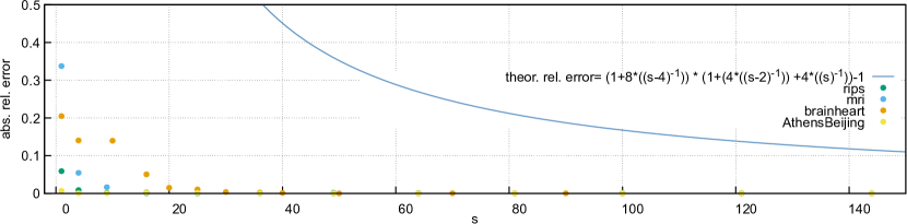
Figure 7: Convergence of PDoptFlow for $W_{1}$-distance against the parameter $s$.

$W_{1}$ Empirical Errors for a given Theoretical Error
PD data sets	Emp. Err. $s=40$ (Ours)	Emp. Err. $\varepsilon=0.5$(hera)	Emp. Err. $s=93$ (Ours)	Emp. Err. $\varepsilon=0.2$(hera)
bh	0.00093	0.00028	0.00014	0.000280
AB	0.00043	0.00101	8.6e-5	0.000233
mri	0.00224	0.00373	0.00077	0.001315
rips	0.00011	0.00689	3.4e-5	0.001770

Table 6: Empirical relative error of PDoptFlow and hera.

$W_{1}$-Distance Computation Stats. for a Guaranteed Rel. Error Bound
PD data sets	%node drop, (#nodes, #arcs) for $W_{40}^{PD}(A^{\delta},B^{\delta})$	%node drop, (#nodes, #arcs) for $W_{90}^{PD}(A^{\delta},B^{\delta})$
bh	90%,(18K,22M)	86%,(25K,92M)
AB	82%,(2.5K,1.4M)	70%,(4.3K,6.1M)
mri	70%,(55K,57M)	67%,(60K,188M)
rips	2%,(68K,133M)	0.3%,(69K,468M)

Table 7: $\delta$-condensation statistics. K: $\times 10^{3}$, M: $\times 10^{6}$.

4.1 Nearest Neighbor Search Experiments

We perform experiments in regard to Problem 2. NN search is an important problem in machine learning [5, 23], content based image retrieval  [58], in high performance computing [78, 65] and recommender systems [68]. We use the dataset given in [22] which consists of 200 PDs coming from graphs generated by the reddit dataset. Having established ground truth with the guaranteed $0.01$ approximation of hera, we proceed to find the nearest neighbor for a given query PD. Following [5], we consider various approximations to the $W_{1}$-distance. We experiment with $6$ different approximations: the Word Centroid Distance (WCD), RWMD [52], quadtree, flowtree [22], PDoptFlow at $s=1$ and PDoptFlow at $s=18$ for a guaranteed $2.3$ factor approximation. The WCD lower bound is achieved with the observation in [22]. Table 3 shows the prediction accuracies and timings of all approximation algorithms considered on the reddit dataset. Sinkhorn or dense network simplex are not considered in our experiments because they require $O(n^{2})$ memory. This is infeasible for large PDs in general.

Although PDoptFlow is fast for the error that it can achieve, the computational time to use PDoptFlow for all comparisions is still too costly, however. This suggests combining the 7 considered algorithms to achieve high performance at the best prediction accuracy. One way of combining algorithms is through pipelining, which we discuss next.

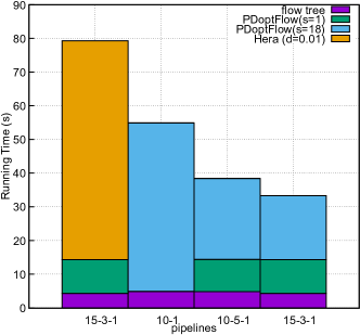
Figure 8: Pipelines for computing NN.

Pipelining Approximation Algorithms: Following [5] and using a distance to compute a set of candidate nearest neighbors, we pipeline these algorithms in increasing order of their accuracy to find the $1$-NN with at least $90\%$ accuracy. A pipeline of $k$ algorithms is written as $c_{1}-c_{2}-\cdots-c_{k}$ where $c_{i}$ is the number of output candidates of the ith algorithm in the pipeline.

Since flowtree achieves a better accuracy than RWMD and WCD in less time, we can eliminate WCD and RWMD from any pipeline experiment. This is illustrated by WCD and RWMD not being on the Pareto frontier in Figure 2. The quadtree algorithm is not worth placing into the pipeline since its accuracy is too low; it prunes the NN as a potential output PD too early. It also can only save on flowtree’s time, which is not the bottleneck of the pipeline. In fact, the last stage of computation, which can only be achieved with a high accuracy algorithm such as hera or PDoptFlow, always forms the bottleneck to computing the NN.

Figure 8 shows four pipelines involving flowtree, PDoptFlow and hera. The 15-3-1 pipeline consisting of Flowtree then PDoptFlow(s=1) and then PDoptFlow(s=18) was found to be the best in performance through grid search. Three other pipelines computed in the grid search are shown. Each pipeline computes 100 queries with at least $90\%$ accuracy for a random split of the reddit dataset. We measure the total amount of time it takes to compute all 100 queries. For the pipeline 15-3-1 with hera replacing PDoptFlow(s=18), hera takes 65 seconds on 3 queries, while PDoptFlow takes 19 seconds on 3 queries. We find that $82\%$ of the time is spent on only $3\%$ of the PDs for hera, while $57\%$ of the time is spent if PDoptFlow($s=18$) replaces hera. We notice that flowtree is able to eliminate a large number of candidate PDs in a very short amount of time though it is not able to complete the task of finding the NN due to its low prediction accuracy. PDoptFlow($s=1$) surprisingly achieves very good times and prediction accuracies without an approximation bound.

5 Conclusion

We propose a new implementation for computing the $W_{1}$-distances between persistence diagrams that provides a $1+O(\varepsilon)$ approximation. We achieve a considerable speedup for a given guaranteed relative error in computation by two algorithmic and implementation design choices. First, we exploit geometric structures effectively via $\delta$-condensation and $s$-WSPD, which sparsify the nodes and arcs, respectively, when comparing PDs. Second, we exploit parallelism in our methods with an implementation in GPU and multicore. Finally, we establish the effectiveness of the proposed approaches in practice by extensive experiments. Our software PDoptFlow can achieve an order of magnitude speedup over other existing software for a given theoretical relative error. Furthermore, PDoptFlow overcomes the computational bottleneck to finding the NN amongst PDs and guarantees an $O(1)$ approximate nearest neighbor. One merit of our algorithm is its applicability beyond comparing persistence diagrams. The algorithm is in fact applicable to an unbalanced optimal transport problem on $\mathbb{R}^{2}$ upon viewing $\bar{b}$ and $\bar{a}$ as creator/destructor and reassigning the diagonal arc distances to the creation/destruction costs.

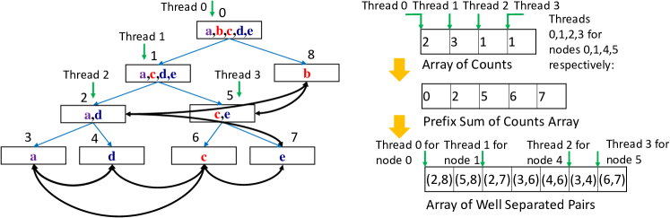
Figure 9: constructing WSPD in parallel for array from the split tree

Appendix A Appendix

Here we present the datasets, algorithms, finer implementation details, more experiments, and discussions that are not presented in the main body of the paper due to the space limit.

A.1 More Algorithmic Details:

Here we present the algorithmic and implementation details that are omitted in the main context of the paper.

A.1.1 WCD:

We implement the WCD using the Observation in [22] that $OT(A\cup\tilde{B},B\cup\tilde{A})\leq 2W_{1}(A,B)$, where $OT(A\cup\tilde{B},B\cup\tilde{A})$ is the classical optimal transport distance between $A\cup\tilde{B}$ and $B\cup\tilde{A}$, the sum of distances of their optimal matching, is a $2$ approximation to $W_{1}(A,B)$. Since WCD$(A\cup\tilde{B},B\cup\tilde{A})\leq\text{OT}(A\cup\tilde{B},B\cup\tilde{A})$, we get $\frac{1}{2}$ WCD$\leq W_{1}(A,B)$.

flowtree is faster than WCD on reddit due to the small scale of the PDs in that dataset. However asymptotically WCD is much faster on very large datasets since it can be implemented as a $O(\log n)$ depth sum-reduction of coordinates on GPU, similar to quadtree.

A.1.2 WSPD and Spanner Construction:

Here we present our simplified parallel algorithm for WSPD construction used in our implementation. The purpose of traversing the split tree twice is to parallelize writing out the WSPD, the bottleneck to constructing a WSPD. Although the WSPD is linear in $n$, the number of nodes of ${\sf WS}_{s}^{PD}(A^{\delta},B^{\delta})$, in practice the size of the WSPD is several orders of magnitude larger than $n$. Thus writing out the WSPD requires a large amount of data movement. Algorithm 5 first finds the number of pairs written out by a thread rooted at some node in the split tree. The computation of counts is in parallel and is mostly arithmetic. Once the counts are accumulated, a prefix sum of the counts is computed and written out to an offsets array. The offsets are then used as starting memory addresses to write out the WSPD pairs for each thread in parallel.

Figure 9 illustrates the parallel computation of the WSPD. The prefix sum is computed over the counts determined by each thread. There is a thread per internal node.

In our implementation, we do not actually keep track of the point subsets for each node of the split tree. Instead, we keep track of a single point in each point subset $P\subset\hat{A}\cup\hat{B}$ as well as a bounding box of $P$. This constructs the non-diagonal arcs of ${\sf WS}_{s}^{PD}(A,B)$ with minimal data.

1:$\boldsymbol{T}$ a split tree, WSPD parameter $s$

2:$s$-$WSPD$ represented by wspd-ptn-pairs as an array

3:counts $\leftarrow\{0...0\}$ $\triangleright$ allocate O(n) elements

4:for node $w\in\boldsymbol{T}$ in parallel do

5:     count-WSPD$(tid(w),$w.left,.w.right,$s$,counts)

6:offsets $\leftarrow$ prefix-sum(counts)

7:$L$= offsets[w] $\triangleright$ offsets[w]=sum(counts)

8:wspd-ptn-pairs $\leftarrow\{...\}$ $\triangleright$ allocate $L$ elements for wspd-ptn-pairs: $O(s^{2}n)$ memory

9:for node $w\in\boldsymbol{T}$ in parallel do

10:     construct-WSPD(tid(w),w.left,w.right,s,offsets, wspd-ptn-pairs)

Algorithm 4 Construct $s$-WSPD-biarcs in parallel

1:function count-WSPD

2:$tid$: thread id; nodes $u$ and $v$ in the split tree; $s$: WSPD parameter; counts: the number of recursive calls made by each thread;

3:counts: array of counts, counts$[tid]$= number of pairs each thread will find

4:     if $u$ is $s$-well separated from $v$ then

5:         counts$[tid]$++ return $\triangleright$ keep track of the number of well separated pairs associated with $tid$      

6:     if $\text{max\_len(BndingBx(u))}>\text{max\_len(BndingBx(v))}$ then

7:         $\text{count-WSPD}(tid,u.\text{left},v,s,$counts)

8:         $\text{count-WSPD}(tid,u.\text{right},v,s,$counts)

9:     else

10:         $\text{count-WSPD}(tid,u,v.\text{left},s,$counts)

11:         $\text{count-WSPD}(tid,u,v.\text{right},s,$counts)      

Algorithm 5 Compute WSPD thread counts for offsets

1:function construct-WSPD

2:$tid$: thread id; nodes $u$ and $v$ in the split tree; $s$: WSPD parameter; offsets: wspd: a writable array of point pairs;

3:$s$-WSPD with representatives of point pairs as an array

4:     if $u$ is $s$-well separated from $v$ then

5:         $wspd[$offsets$[tid]$++] $\leftarrow(u.\text{point},v.\text{point})$ $\triangleright$ all threads write in parallel return      

6:     if max_len(BndingBx($u$))$>$max_len(BndingBx) then

7:         $\text{construct-WSPD}(tid,u.\text{left},v,s,$wspd)

8:         $\text{construct-WSPD}(tid,u.\text{right},v,s,$wspd)

9:     else

10:         $\text{construct-WSPD}(tid,u,v.\text{left},s,$wspd)

11:         $\text{construct-WSPD}(tid,u,v.\text{right},s,$wspd)      

Algorithm 6 Write out WSPD from offsets

Algorithm 7 shows how to write out the diagonal arcs for ${\sf WS}_{s}^{PD}(A^{\delta},B^{\delta})$. On line 2 it states that there is a parallelization by prefix sum on arc counts. This computation is similar to the algorithm for WSPD construction. The number of arcs per point is kept track of. A prefix sum is computed after this and the diagonal arcs are written out per point.

1:for point $p\in\boldsymbol{P}=\hat{A}_{\delta}\cup\hat{B}_{\delta}$ parallelized by prefix sum on count of arcs incident on each $p$ do

2:     if p is from $\hat{A}_{\delta}$ then diag-arcs $\leftarrow$ diag-arcs $\cup\{p,p_{proj}\}$      

3:     if p is from $\hat{B}_{\delta}$ then diag-arcs $\leftarrow$ diag-arcs $\cup\{p_{proj},p\}$      

Algorithm 7 Form diagonal arcs

A.1.3 Assumptions on PD density for $\delta$-condensation

Proposition 2 has $\delta=O(\frac{1}{n})$ where $n$ is the total number of points of both PDs. In particular, assuming $W_{1}(A,B)$ bounded, we have $\delta\rightarrow 0$ as $n\rightarrow\infty$. In order for $\delta$-condensation to scale with $n$, we need to make an appropriate assumption about the distribution of points for our PDs. Define the density for a point set $A\subset\mathbb{R}^{2}$ on a $\delta$-square grid as $\frac{|A|}{|\Gamma_{\delta}|}$ where $|\Gamma_{\delta}|$ is the number of nonempty grid cells with points from $A$.

Proposition A.1.

The fraction of nodes eliminated from $A$ by $\delta$-condensation increases if the density of a PD $A$ on a $\delta$-grid increases.

Proof.

For each grid point $p\in\Gamma_{\delta}$, all points in a $\delta$-square neighborhood centered at $p$ snap to $p$. These new cells partition the plane just like the original grid cells and are a translation of the original grid cells. We consider this translated grid as $\Gamma_{\delta}$, which can only affect the number of nonempty cells by at most a factor of $4$. Say a $\delta$-cell $i\in\Gamma_{\delta}$, $\delta$ depending on $|A|$, has $c_{i}$ points. We get that exactly $c_{i}$ points collapse into one point. Thus $c_{i}-1$ points are eliminated. Adding this up over all nonempty cells $i$, we get that the fraction of nodes eliminated from $A$ is:

$$\frac{\sum_{i\in\Gamma_{\delta}}(c_{i}-1)}{|A|}=\frac{|A|-|\Gamma_{\delta}|}{|A|}$$

It follows that if the density $\frac{|A|}{|\Gamma_{\delta}|}$ increases, we eliminate a larger fraction of nodes as claimed. ∎

In particular, for lower star filtrations on voxel based data, we have that there are only $2^{8}$ possible number of filtration values to fill up, up to infinitesimal perturbations from the data. We thus have, $|\Gamma_{\delta}|\leq 2^{16}$ for all $\delta$, where $2^{16}$ counts the bound on the number of pairs of filtration values that lie in $\mathbb{R}^{2}$. Then, by Proposition A.1, $\delta$-condensation scales well when $n$ is sufficiently large. For lower star filtrations defined on degree valued nodes of scale free networks, the degree distribution is given by the power law: $P(k)\sim k^{-\gamma}$, $2<\gamma<3$ a constant and $k$ the degree of any node. Thus, as $n\rightarrow\infty$, we sample at most $n$ times from this distribution. With probability 0.99, each sample is bounded by some constant threshold $N(\gamma)=O((\frac{1}{0.99})^{\frac{1}{\gamma}})$. Hence, $|\Gamma_{\delta}|$ is bounded w.h.p. and by Proposition A.1, we have that $\delta$-condensation eliminates an eventually increasing proportion of nodes w.h.p. as $n\rightarrow\infty$.

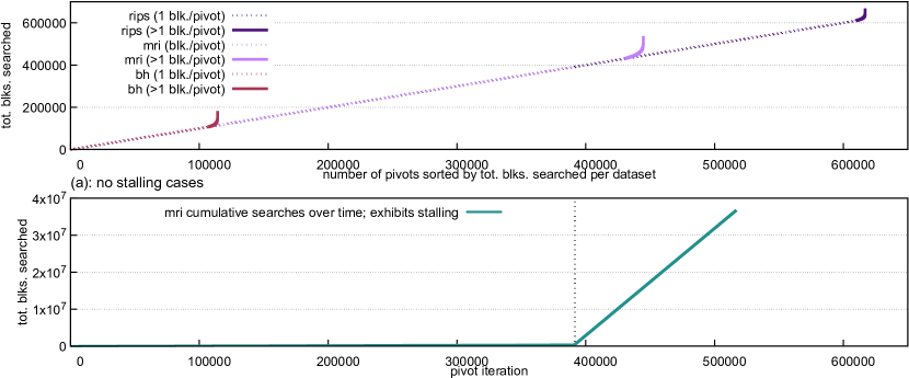
Figure 10: (a) Plot of no stalling case of the cumulative distribution of blocks searched for rips, mri and brain-heart datasets. (b) Plot of a stalling case for the mri dataset. block size= $\sqrt{m}$

A.1.4 Representing the Transshipment Network:

The data structure used to represent the transshipment network significantly affects the performance of network simplex algorithm. Since most of the time of computation is spent on the network simplex algorithm and not the network construction stage, the network data structure is designed to be constructed to be as efficient for arc reading and updating as possible. A so-called static graph representation [33], essentially a compressed sparse row (CSR) [38] format matrix, is used to represent the transshipment network. Thus in order to build a CSR matrix, we must sort the arcs $(u,v)$ first by first node followed by second node in case of ties. This sorting can be over several millions of arcs, see Table 2 column 2. For example, for rips at $\varepsilon^{\prime}\leq 0.2$, 468 million arcs must be sorted. ($\varepsilon^{\prime}$ is the guaranteed relative error bound). For a sequential $O(m\log m)$ algorithm, this would form a bottleneck to the entire algorithm before network simplex, making the algorithm $\Omega(m\log(m))$. Thus we sort the arcs on GPU using the standard parallel merge sorting algorithm [11, 26] and achieving a parallel depth complexity of $O(\log m)$.

A.2 Computational Behavior of Network Simplex (BSP in practice):

Refer to Section 4 and Table 5 for dataset information. Figure 10 shows two very different computational patterns of the block search pivot based NtSmplx algorithm. Figure 10(a) shows the vast majority of cases when there is no stalling. We show the cumulative distribution of blocks searched for the rips, mri and brain-heart datasets at s=20, 49 and 150 respectively. The block sizes are set to the square root of the number of arcs; the block sizes are 6539, 9134 and 8922 respectively. Notice that 98.9%, 96.8% and 93.8% of the pivots involve only a single block being searched, and account for 91.4%, 80.2% and 58.8% of the total blocks searched. Although the pivots are sorted per dataset by the number of blocks searched, the cumulative distribution depending on the pivots computed over execution is almost identical. Figure 10(b) shows the relatively rare but severe case of stalling for the mri dataset at s=36, stopped after 10 minutes. Stalling begins at the 391559th arc found.

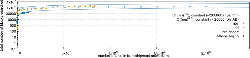
Figure 11: Plot of the total number of block pivot searches depending on the number of arcs.

Furthermore, we have noticed empirically that repeated tie breaking of reduced costs during pivot searching results in a tendency to stall. In fact, most implementations simply repeatedly choose the smallest indexed arc for tie breaking. After applying lattice snapping by $\pi_{\delta}$, symmetry is introduced into the pairwise relationships and thus results in many equivalent costs on arcs and subsequent reduced costs. This is why we introduce a small perturbation to the snapped points in order to break this symmetry. This results in much less stalling in practice.

A.2.1 Parallelizing Network Simplex Algorithm:

Network simplex is a core algorithm used for many computations, especially exact optimal transport. This introduces a natural question: can we directly parallelize some known network simplex pivot search strategies and gain a performance improvement? We attempted to implement parallel pivot search strategies such as a $O(\log m)$-depth parallel min reduction over all reduced costs on either GPU or multicore, such as in [67]. These approaches did not improve performance over a sequential block pivot search strategy. There was speedup over Dantzig’s pivot strategy, where all admissible arcs are checked, however. For GPU, there is an issue of device to host and host to device memory copy. These IO operations dominate the pivot searching phase and are several of orders of magnitude slower than a single block searched sequentially from our experiments. Recall that most searches result in a single block by Figure 10. For multicore, there is an issue of thread scheduling which provides too much overhead. In general, it is very difficult to surpass the performance of a sequential search over a single block when the block size can fit in the lower level cache due to the two aforementioned issues. For example, in our experiments the cache size is 28160KB, which should hold $6\cdot B\cdot 8$ bytes for $B=\sqrt{m}$, the block size, and $m<3\times 10^{11}$ where 6 denotes the 6 arrays needed to be accessed to compute the reduced cost and 8 is the number of bytes in a double. This bound on $m$, the number of arcs, should hold for almost all pairs of conceivable input persistence diagrams and $s>0$ in practice. This does not preclude, however the possibility of efficient parallel pivoting strategies completely since stalling still exists for the sequential block search algorithm.

A.2.2 Empirical Complexity:

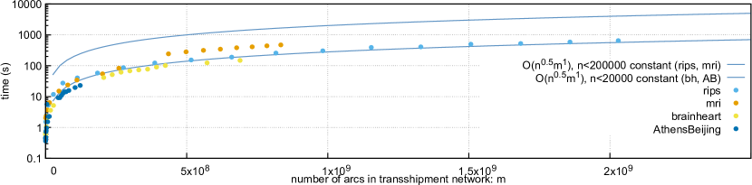
Figure 12: Plot of the empirical time (log scale) depending on the number of arcs of the sparsified transshipment network for each dataset. $n$ is the number of nodes.

For each of the datasets from Table 5, our experiments illustrated in Figure 12, show that for varying $s$ and fixed $n$, our overall approach runs empirically in $O(\sqrt{n}m)$ time, where $m=s^{2}n$ with $s$ the WSPD parameter and $n$ the number of nodes in the sparsified transshipment network.

Here we explain in more detail the experiment illustrated in Figure 1. We determine the empirical complexity with respect to the number of points on a synthetic Gaussian dataset. These are not real persistence diagrams and are made up of points randomly distributed on the plane above the diagonal. The points follow a Gaussian distribution. For fixed $s\leq 40$, as a function of $n$ our algorithm empirically is upper bounded by $O(s^{2}n^{1.5})$. This is determined through upper bounding the least squares curve fitting. Since we are still solving a linear program, it should not be expected that the empirical complexity can be truly linear, except perhaps under certain dataset conditions. The proximity of points, for certain real persistence diagrams, for example, could be exploited more by $\delta$-condensation. We notice that the empirical complexity is better, the smaller the $s$, including for $s\leq 40$. This is why in Section 4 PDoptFlow for $s=1$ performs so much faster than PDoptFlow for $s=18$.

A.2.3 Stopping Criterion:

Due to the rareness of stalling for given $s$ in practice, our stopping criterion is designed to justify the empirical time bound. If the block size is $\sqrt{m}$, the computation goes like $O(s^{2}n^{1.5})$, and each iteration within a block search determines the time, $O(\frac{s^{2}n^{1.5}}{s\sqrt{n}})=O(\sqrt{mn})$ blocks is an upper bound on the number of searched blocks when there is no stalling. Figure 11 illustrates this relationship amongst $m$, $n$ and the time. Thus the stopping criterion is set to $C\sqrt{mn}+b$. In practice, $C$ may simply be set to $0$ and $b$ set to a large number however it has been empirically found that the stopping citerion goes like $\sqrt{mn}$ blocks for a large number of the various types of real persistence diagrams such as those generated by the persistence algorithm on lower star filtrations induced by images and rips filtrations on random point clouds, to name the types from the experiments.

A.2.4 Bounds on Min-Cost Flow:

The $W_{1}$-distance between PDs is a special case of the unbalanced optimal transport (OT) problem as formulated in [53, 70]. Solving such a problem exactly using min-cost flow is known to take cubic complexity [66] in the number of points. However, affording cubic complexity is usually infeasible in practice and thus we seek a subcubic solution.

There are several approaches to approximating the distance between PDs with $n$ total points. In [22], a $\log\Delta$ approximation is developed, where, $\Delta$ is the aspect ratio, adapting the work of [47] and [5] for persistence diagrams. In [50], the auction matching algorithm performs a $(1+\varepsilon)$ approximation, also lowering complexity by introducing geometry into the computation. Geometry lowers a linear search over $O(n)$ points for nearest neighbors to $O(\sqrt{n})$ via kd-tree. This does not lower the theoretical bound below $O(n^{2.5})$, however. Our approach lowers complexity by introducing a geometric spanner [14], using a linear number of arcs between points.

Min-cost flow algorithms can have theoretically very low complexity. The input to min-cost flow is a transshipment network and its output is the minimum cost flow value. Let $m$ be the number of arcs in the transshipment network and $n$ its number of nodes. It was shown that min-cost flow can be found exactly in $\tilde{O}(m+n^{1.5})$ complexity in [12], by network simplex in $\tilde{O}(n^{2})$ complexity, in parallel in $\tilde{O}(\sqrt{m})$ and approximated on undirected graphs in [8] in $\tilde{O}(m^{1+o(1)})$ complexity.

Since the number of nodes and arcs of the transshipment network depend directly on the points and pairwise distances respectively, an implication of using a geometric spanner for $(1+O(\varepsilon))$ approximation is that the complexity becomes theoretically subcubic and requiring $O_{\varepsilon}(n)$ memory, where $O_{\varepsilon}$ hides a polynomial dependency on $\epsilon$, the relative approximation error. In fact this bound is actually achieved in practice. We show the empirical complexity is actually similar to $O(s^{2}n^{1.5})$ as shown in Figure 12 and Figure 1 but only for small $s$.

References

- [1] Charu C. Aggarwal, Haim Kaplan, and Robert E. Tarjan. A faster primal network simplex algorithm. 1996.
- [2] James Ahrens, Berk Geveci, and Charles Law. Paraview: An end-user tool for large data visualization. The Visualization Handbook, 717, 2005.
- [3] Alexander Andreopoulos and John K. Tsotsos. Efficient and generalizable statistical models of shape and appearance for analysis of cardiac mri. Medical Image Analysis, 12(3):335–357, 2008.
- [4] Kubilay Atasu and Thomas Mittelholzer. Linear-complexity data-parallel earth mover’s distance approximations. In International Conference on Machine Learning, pages 364–373. PMLR, 2019.
- [5] Arturs Backurs, Yihe Dong, Piotr Indyk, Ilya Razenshteyn, and Tal Wagner. Scalable nearest neighbor search for optimal transport. In International Conference on Machine Learning, pages 497–506. PMLR, 2020.
- [6] Albert-László Barabási and Réka Albert. Emergence of scaling in random networks. Science, 286(5439):509–512, 1999.
- [7] Ulrich Bauer. Ripser: efficient computation of Vietoris-Rips persistence barcodes. arXiv preprint arXiv:1908.02518, 2019.
- [8] Aaron Bernstein, Maximilian Probst Gutenberg, and Thatchaphol Saranurak. Deterministic decremental sssp and approximate min-cost flow in almost-linear time. arXiv preprint arXiv:2101.07149, 2021.
- [9] Dimitri P. Bertsekas. The auction algorithm: A distributed relaxation method for the assignment problem. Annals of Operations Research, 14(1):105–123, 1988.
- [10] Robert G. Bland. New finite pivoting rules for the simplex method. Mathematics of operations Research, 2(2):103–107, 1977.
- [11] Guy E. Blelloch and Bruce M. Maggs. Parallel algorithms. In Algorithms and Theory of Computation Handbook: Special Topics and Techniques, pages 25–25. 2010.
- [12] Jan van den Brand, Yin Tat Lee, Yang P Liu, Thatchaphol Saranurak, Aaron Sidford, Zhao Song, and Di Wang. Minimum cost flows, MDPs, and -regression in nearly linear time for dense instances. arXiv preprint arXiv:2101.05719, 2021.
- [13] Rainer Burkard, Mauro Dell’Amico, and Silvano Martello. Assignment problems: revised reprint. SIAM, 2012.
- [14] Sergio Cabello, Panos Giannopoulos, Christian Knauer, and Günter Rote. Matching point sets with respect to the earth mover’s distance. In European Symposium on Algorithms, pages 520–531. Springer, 2005.
- [15] Paul B. Callahan. Optimal parallel all-nearest-neighbors using the well-separated pair decomposition. In Proceedings of 1993 IEEE 34th Annual Foundations of Computer Science, pages 332–340. IEEE, 1993.
- [16] Paul B. Callahan and S. Rao Kosaraju. A decomposition of multidimensional point sets with applications to k-nearest-neighbors and n-body potential fields. Journal of the ACM (JACM), 42(1):67–90, 1995.
- [17] Mathieu Carrière, Marco Cuturi, and Steve Oudot. Sliced wasserstein kernel for persistence diagrams. In International conference on machine learning, pages 664–673. PMLR, 2017.
- [18] Ohio Supercomputer Center. Pitzer supercomputer, 2018. URL: http://osc.edu/ark:/19495/hpc56htp.
- [19] Deeparnab Chakrabarty and Sanjeev Khanna. Better and simpler error analysis of the sinkhorn–knopp algorithm for matrix scaling. Mathematical Programming, pages 1–13, 2020.
- [20] Timothy M. Chan. Well-separated pair decomposition in linear time? Information Processing Letters, 107(5):138–141, 2008.
- [21] Frédéric Chazal, Vin de Silva, and Steve Oudot. Persistence stability for geometric complexes. Geometriae Dedicata, 173(1):193–214, 2014.
- [22] Samantha Chen and Yusu Wang. Approximation algorithms for 1-wasserstein distance between persistence diagrams. arXiv preprint arXiv:2104.07710, 2021.
- [23] Yihua Chen, Eric K. Garcia, Maya R. Gupta, Ali Rahimi, and Luca Cazzanti. Similarity-based classification: Concepts and algorithms. Journal of Machine Learning Research, 10(3), 2009.
- [24] Ken Clarkson. Approximation algorithms for shortest path motion planning. In Proceedings of the Nineteenth Annual ACM Symposium on Theory of Computing, pages 56–65, 1987.
- [25] David Cohen-Steiner, Herbert Edelsbrunner, and John Harer. Stability of persistence diagrams. Discrete & computational geometry, 37(1):103–120, 2007.
- [26] Richard Cole. Parallel merge sort. SIAM Journal on Computing, 17(4):770–785, 1988.
- [27] Marco Cuturi. Sinkhorn distances: Lightspeed computation of optimal transport. In Advances in neural information processing systems, pages 2292–2300, 2013.
- [28] George B. Dantzig and Mukund N. Thapa. Linear programming 2: theory and extensions. Springer Science & Business Media, 2006.
- [29] Thomas Davies, Jack Aspinall, Bryan Wilder, and Long Tran-Thanh. Fuzzy c-means clustering for persistence diagrams. arXiv preprint arXiv:2006.02796, 2020.
- [30] Jean-Lou De Carufel, Prosenjit Bose, Frédérik Paradis, and Vida Dujmovic. Local routing in WSPD-based spanners. Journal of Computational Geometry, 12(1):1–34, 2021.
- [31] Tamal K. Dey, Jiayuan Wang, and Yusu Wang. Graph reconstruction by discrete Morse theory. In Proceedings 34th International Symposium on Computational Geometry (SoCG), pages 31:1–31:15, 2018.
- [32] Tamal K. Dey and Yusu Wang. Computational topology for Data Analysis. Cambridge University Press, 2022. URL: https://www.cs.purdue.edu/homes/tamaldey/book/CTDAbook/CTDAbook.html.
- [33] Balázs Dezső, Alpár Jüttner, and Péter Kovács. Lemon–an open source c++ graph template library. Electronic Notes in Theoretical Computer Science, 264(5):23–45, 2011.
- [34] Vincent Divol and Théo Lacombe. Understanding the topology and the geometry of the persistence diagram space via optimal partial transport. arXiv preprint arXiv:1901.03048, 2019.
- [35] Herbert Edelsbrunner and John Harer. Computational Topology: An Introduction. American Mathematical Society, 2010.
- [36] Herbert Edelsbrunner, David Letscher, and Afra Zomorodian. Topological persistence and simplification. In Proceedings 41st Annual Symposium on Foundations of Computer Science, pages 454–463. IEEE, 2000.
- [37] Brian L. Edlow, Azma Mareyam, Andreas Horn, Jonathan R. Polimeni, Thomas Witzel, M. Dylan Tisdall, Jean C. Augustinack, Jason P. Stockmann, Bram R. Diamond, Allison Stevens, et al. 7 Tesla MRI of the ex vivo human brain at 100 micron resolution. Scientific data, 6(1):1–10, 2019.
- [38] Stanley C. Eisenstat, Howard C. Elman, Martin H. Schultz, and Andrew H. Sherman. The (new) Yale sparse matrix package. In Elliptic Problem Solvers, pages 45–52. Elsevier, 1984.
- [39] Andreas Fabri and Sylvain Pion. Cgal: The computational geometry algorithms library. In Proceedings of the 17th ACM SIGSPATIAL international conference on advances in geographic information systems, pages 538–539, 2009.
- [40] Brittany Terese Fasy, Xiaozhou He, Zhihui Liu, Samuel Micka, David L. Millman, and Binhai Zhu. Approximate nearest neighbors in the space of persistence diagrams. arXiv preprint arXiv:1812.11257, 2018.
- [41] R’emi Flamary and Nicolas Courty. POT python optimal transport library, 2017. URL: https://pythonot.github.io/.
- [42] Andrew V. Goldberg, Michael D. Grigoriadis, and Robert E. Tarjan. Efficiency of the network simplex algorithm for the maximum flow problem. Technical report, Princeton Univ., Dept. Computer Science, 1988.
- [43] Michael D. Grigoriadis. An efficient implementation of the network simplex method. In Netflow at Pisa, pages 83–111. Springer, 1986.
- [44] Joachim Gudmundsson, Christos Levcopoulos, and Giri Narasimhan. Fast greedy algorithms for constructing sparse geometric spanners. SIAM Journal on Computing, 31(5):1479–1500, 2002.
- [45] Sariel Har-Peled. Geometric approximation algorithms. Number 173. American Mathematical Soc., 2011.
- [46] Charles R. Harris, K. Jarrod Millman, St’efan J. van der Walt, Ralf Gommers, Pauli Virtanen, David Cournapeau, Eric Wieser, Julian Taylor, Sebastian Berg, Nathaniel J. Smith, Robert Kern, Matti Picus, Stephan Hoyer, Marten H. van Kerkwijk, Matthew Brett, Allan Haldane, Jaime Fern’andez del R’ıo, Mark Wiebe, Pearu Peterson, Pierre G’erard-Marchant, Kevin Sheppard, Tyler Reddy, Warren Weckesser, Hameer Abbasi, Christoph Gohlke, and Travis E. Oliphant. Array programming with NumPy. Nature, 585(7825):357–362, September 2020. doi:10.1038/s41586-020-2649-2.
- [47] Piotr Indyk and Nitin Thaper. Fast image retrieval via embeddings. In 3rd international workshop on statistical and computational theories of vision, volume 2, page 5, 2003.
- [48] Roy Jonker and Ton Volgenant. Improving the Hungarian assignment algorithm. Operations Research Letters, 5(4):171–175, 1986.
- [49] J. Mark Keil. Approximating the complete euclidean graph. In Scandinavian Workshop on Algorithm Theory, pages 208–213. Springer, 1988.
- [50] Michael Kerber, Dmitriy Morozov, and Arnur Nigmetov. Geometry helps to compare persistence diagrams. Journal of Experimental Algorithmics (JEA), 22:1–20, 2017.
- [51] Zoltán Király and Péter Kovács. Efficient implementations of minimum-cost flow algorithms. arXiv preprint arXiv:1207.6381, 2012.
- [52] Matt Kusner, Yu Sun, Nicholas Kolkin, and Kilian Weinberger. From word embeddings to document distances. In International conference on machine learning, pages 957–966. PMLR, 2015.
- [53] Théo Lacombe, Marco Cuturi, and Steve Oudot. Large scale computation of means and clusters for persistence diagrams using optimal transport. In Advances in Neural Information Processing Systems, pages 9770–9780, 2018.
- [54] Richard E. Ladner and Michael J. Fischer. Parallel prefix computation. Journal of the ACM (JACM), 27(4):831–838, 1980.
- [55] Hung Le and Shay Solomon. Light euclidean spanners with steiner points. arXiv preprint arXiv:2007.11636, 2020.
- [56] Tam Le and Truyen Nguyen. Entropy partial transport with tree metrics: Theory and practice. arXiv preprint arXiv:2101.09756, 2021.
- [57] Yin Tat Lee and Aaron Sidford. Path finding ii: An~ o (m sqrt (n)) algorithm for the minimum cost flow problem. arXiv preprint arXiv:1312.6713, 2013.
- [58] Michael S. Lew, Nicu Sebe, Chabane Djeraba, and Ramesh Jain. Content-based multimedia information retrieval: State of the art and challenges. ACM Transactions on Multimedia Computing, Communications, and Applications (TOMM), 2(1):1–19, 2006.
- [59] Fredrik Manne and Mahantesh Halappanavar. New effective multithreaded matching algorithms. In 2014 IEEE 28th International Parallel and Distributed Processing Symposium, pages 519–528. IEEE, 2014.
- [60] Andrew Marchese, Vasileios Maroulas, and Josh Mike. K- means clustering on the space of persistence diagrams. In Wavelets and Sparsity XVII, volume 10394, page 103940W. International Society for Optics and Photonics, 2017.
- [61] Clément Maria, Jean-Daniel Boissonnat, Marc Glisse, and Mariette Yvinec. The Gudhi library: Simplicial complexes and persistent homology. In International Congress on Mathematical Software, pages 167–174. Springer, 2014.
- [62] Dmitriy Morozov. Dionysus software. Retrieved December, 24:2018, 2012.
- [63] Brendan Mumey. Indexing point sets for approximate bottleneck distance queries. arXiv preprint arXiv:1810.09482, 2018.
- [64] Chris Tralie Nathaniel Saul. Scikit-tda: Topological data analysis for python, 2019. doi:10.5281/zenodo.2533369.
- [65] Sameer A. Nene and Shree K. Nayar. A simple algorithm for nearest neighbor search in high dimensions. IEEE Transactions on pattern analysis and machine intelligence, 19(9):989–1003, 1997.
- [66] James B. Orlin. A faster strongly polynomial minimum cost flow algorithm. Operations research, 41(2):338–350, 1993.
- [67] Nikolaos Ploskas and Nikolaos Samaras. GPU accelerated pivoting rules for the simplex algorithm. Journal of Systems and Software, 96:1–9, 2014.
- [68] Ali M. Roumani and David B. Skillicorn. Finding the positive nearest-neighbor in recommender systems. In DMIN, pages 190–196, 2007.
- [69] Yossi Rubner, Carlo Tomasi, and Leonidas J. Guibas. The earth mover’s distance as a metric for image retrieval. International journal of computer vision, 40(2):99–121, 2000.
- [70] Ryoma Sato, Makoto Yamada, and Hisashi Kashima. Fast unbalanced optimal transport on tree. arXiv preprint arXiv:2006.02703, 2020.
- [71] Primoz Skraba and Katharine Turner. Wasserstein stability for persistence diagrams. arXiv preprint arXiv:2006.16824, 2020.
- [72] Anirudh Som, Kowshik Thopalli, Karthikeyan Natesan Ramamurthy, Vinay Venkataraman, Ankita Shukla, and Pavan Turaga. Perturbation robust representations of topological persistence diagrams. In Proceedings of the European Conference on Computer Vision (ECCV), pages 617–635, 2018.
- [73] Roberto Souza, Oeslle Lucena, Julia Garrafa, David Gobbi, Marina Saluzzi, Simone Appenzeller, Letícia Rittner, Richard Frayne, and Roberto Lotufo. An open, multi-vendor, multi-field-strength brain mr dataset and analysis of publicly available skull stripping methods agreement. NeuroImage, 170:482–494, 2018.
- [74] Robert E. Tarjan. Dynamic trees as search trees via euler tours, applied to the network simplex algorithm. Mathematical Programming, 78(2):169–177, 1997.
- [75] Christopher Tralie, Nathaniel Saul, and Rann Bar-On. Ripser. py: A lean persistent homology library for python. Journal of Open Source Software, 3(29):925, 2018.
- [76] Fan Wang, Huidong Liu, Dimitris Samaras, and Chao Chen. TopoGAN: A topology-aware generative adversarial network.
- [77] Yiqiu Wang, Shangdi Yu, Yan Gu, and Julian Shun. Fast parallel algorithms for euclidean minimum spanning tree and hierarchical spatial clustering. In Proceedings of the 2021 International Conference on Management of Data, pages 1982–1995, 2021.
- [78] Bo Xiao and George Biros. Parallel algorithms for nearest neighbor search problems in high dimensions. SIAM Journal on Scientific Computing, 38(5):S667–S699, 2016.
- [79] Simon Zhang, Mengbai Xiao, and Hao Wang. GPU-accelerated computation of Vietoris-Rips persistence barcodes. In 36th International Symposium on Computational Geometry (SoCG 2020). Schloss Dagstuhl-Leibniz-Zentrum für Informatik, 2020.