Stabilising viscous extensional flows using Reinforcement Learning

Abstract

The four-roll mill, wherein four identical cylinders undergo rotation of identical magnitude but alternate signs, was originally proposed by GI Taylor to create local extensional flows and study their ability to deform small liquid drops. Since an extensional flow has an unstable eigendirection, a drop located at the flow stagnation point will have a tendency to escape. This unstable dynamics can however be stabilised using, e.g., a modulation of the rotation rates of the cylinders. Here we use Reinforcement Learning, a branch of Machine Learning devoted to the optimal selection of actions based on cumulative rewards, in order to devise a stabilization algorithm for the four-roll mill flow. The flow is modelled as the linear superposition of four two-dimensional rotlets and the drop is treated as a rigid spherical particle smaller than all other length scales in the problem. Unlike previous attempts to devise control, we take a probabilistic approach whereby speed adjustments are drawn from a probability density function whose shape is improved over time via a form of gradient ascent know as Actor-Critic method. With enough training, our algorithm is able to precisely control the drop and keep it close to the stagnation point for as long as needed. We explore the impact of the physical and learning parameters on the effectiveness of the control and demonstrate the robustness of the algorithm against thermal noise. We finally show that Reinforcement Learning can provide a control algorithm effective for all initial positions and that can be adapted to limit the magnitude of the flow extension near the position of the drop.

I Introduction

In his landmark 1934 paper, and one of his most cited works, GI Taylor proposed a device to study drop deformation and breakup in a two-dimensional flow taylor1934formation . Now called the four-roll mill higdon1993kinematics , the apparatus used electrical motors to rotate four identical cylinders immersed in a viscous fluid. Spinning all cylinders at the same speed (in magnitude), with adjacent cylinders rotating in opposite directions, led to an approximately extensional flow with a stagnation point at the centre. Taylor aimed to study how the extension rate of the flow deformed the drop, when this was placed and kept stable at the stagnation point.

The stagnation point at the centre of an extensional flow is a saddle. The unstable nature of the stagnation point made the drop in Taylor’s experiment difficult to control, and the speed had to be varied in real time to compensate for the drop moving off in the wrong direction taylor1934formation . Over fifty years later, a more systematic method to stabilize the motion of the drop was proposed by Bentley and Leal bentley1986experimental . Using a camera to measure the drift of the drop and computer activated stepping motors to adjust the revolution rates, they modulated the rotation speeds of the cylinders using a simple feedback model where the position of the stagnation point was the control variable.

This newly discovered control scheme allowed further advances in our understanding of capillary flows eggers1997nonlinear , in particular the deformation of drops in shear flows rallison1984deformation . In more recent work, microfluidic devices have been used to control the deformation of small drops  stone2004engineering ; SquireQuake_MicrofluidReview2005 . In particular, microfluidic implementations of the four-roll mill hudson2004microfluidic ; lee2007microfluidic and of related Stokes traps tanyeri2010hydrodynamic ; tanyeri2011microfluidic ; shenoy2016stokes have led to pioneering techniques for trapping and manipulating on small scales.

It is a simple mathematical exercise to show that an extension flow is unstable. Approximating the small drop by a point particle, its trajectory in the steady flow field $\boldsymbol{u}(\boldsymbol{x})$ is solution to $\dot{\boldsymbol{x}}=\boldsymbol{u}(\boldsymbol{x})$. If the centre of the apparatus is used as the origin of the coordinate system $\boldsymbol{0}$, we have $\boldsymbol{u}(\boldsymbol{0})=\boldsymbol{0}$ by symmetry and can therefore approximate $\dot{\boldsymbol{x}}\approx\nabla\boldsymbol{u}(\boldsymbol{0})\cdot\boldsymbol{x}$ near the origin. The extensional flow is irrotational and, since the flow is incompressible, the tensor $\nabla\boldsymbol{u}$ is symmetric and traceless. Therefore, it has real eigenvalues of identical magnitude but opposite sign, $\lambda>0$, and $-\lambda<0$. The centre of the extension flow is thus a saddle point, with basin of attraction parallel to the unidirectional compression and instability in all other directions (see streamlines in Fig. 1).

In this paper, we aim to design a different type of algorithm to drive the drop back when it drifts in the unstable direction. The natural way to correct the trajectory is to adjust the angular rotation rates of the cylinders, but to do so deterministically requires a control model describing the response of the drop to changes in the flow field and for that control scheme to be implemented in real time. This was the rationale for the algorithm proposed in Ref. bentley1986computer using the position of the stagnation point as the control variable. In this paper, instead of a physics-based control scheme we devise a stabilization algorithm using the framework of Reinforcement Learning sutton2018reinforcement .

Reinforcement Learning is a branch of Machine Learning that allows a software agent to behave optimally in a given environment (state space) via observation of environmental feedback. In essence, the agent explores the environment by taking actions (which can be anything from moves in chess to steering in a self-driving car) and receiving positive or negative feedback accordingly. Feedback comes in the form of rewards, which, when suitably added together, make up the return associated with the overall performance. The goal of Reinforcement Learning is, in general, to learn how to maximize this return by improving the agent’s behaviour sutton2018reinforcement . The learning algorithms designed to achieve this vary significantly depending on the nature of the state space (e.g. continuous or discrete, finite or infinite) and on the agent’s knowledge of the effect of actions. When only finitely many actions are available, finding the best behaviour is often entirely algorithmic. If however there is a continuum of states and actions, exploration is typically harder and local improvements to the behaviour have to be found via gradient methods.

Reinforcement Learning has found countless applications in recent years, with significant impact already in fluid dynamics brenner2019perspective ; brunton2020machine . For applications in flow physics at high Reynolds number, Reinforcement Learning has been used for bulk flow control gueniat2016statistical ; rabault2019artificial , the control of free surfaces xie2021sloshing and liquid films belus2019exploiting , shape optimization viquerat2021direct , turbulence modelling novati2021automating and sensor placement paris2021robust . Biological and bio-inspired applications at high high Reynolds numbers include control and energy optimization in fish swimming gazzola2016learning ; novati2017synchronisation ; verma2018efficient , gliding and perching novati2019controlled and locomotion in potential flows jiao2021learning . A landmark study even demonstrated how to exploit Reinforcement Learning in experimental conditions for turbulent drag reduction in flow past bluff bodies fan2020reinforcement . Applications in the absence of inertia have been motivated by biological problems in navigation and locomotion, and include optimal navigation and escape of self-propelled swimmers colabrese2017flow ; gustavsson2017finding ; colabrese2018smart , learning to swim  tsang2020self ; liu2021mechanical and to perform chemotaxis hartl2021microswimmers or even active cloaking mirzakhanloo_esmaeilzadeh_alam_2020 . Reinforcement Learning was also incorporated in experiments using artificial microswimmers navigating in noisy environments muinos2021reinforcement .

In our study, we show how to use the framework of Reinforcement Learning to successfully control the position of a drop in a model of the four-roll mill setup. The flow is modelled as the linear superposition of four two-dimensional rotlets and the drop treated as a rigid spherical particle smaller than all other length scales in the problem. Our state space is a small neighbourhood of the unstable equilibrium in the resulting two-dimensional extension flow, and our actions consist of varying the speed of the cylinders at each time step. We reward actions depending on whether the speed adjustment moves us towards the origin during the time step. Since this is a low-Reynolds-number setup, we can assume that the flow and the drop both respond instantaneously to speed modulation, so that the outcome of an action depends only on the drop’s current position, and not on its current speed or acceleration. The chosen learning algorithm is a classic Actor-Critic method based on gradient ascent. Actions are determined by a set of parameters that are varied, at every time step, in the direction of an estimate of the gradient of performance with respect to these parameters

After introducing the flow model in §II, we give a quick overview of Reinforcement Learning in §III along with a description of our algorithm. The various physical and learning parameters are summarised in §IV. We then demonstrate in §V that, with the right choice of parameters, our algorithm is effective at stabilising the drop from any initial drift. Next, in §VI, we explore the impact of the various physical and learning parameters on the effectiveness of the algorithm. Finally, in §VII we address the robustness of the algorithm against thermal noise, its ability to provide a global policy for all initial positions, and how to modify the algorithm to enable control of the magnitude of the flow extension near the position of the drop.

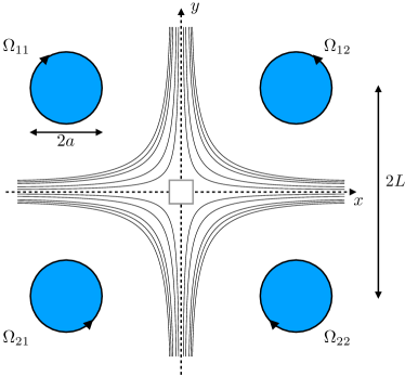
Figure 1: Schematic representation of the four-roll mill setup where four rotating cylinders of radius $a$ and located on a square of side length $2L$ create an extensional flow near the centre of the ($x,y$) coordinate system. The angular velocities of the cylinders are denoted by $\Omega_{ij}$, with $i,j=1,2$. The goal of our Reinforcement Learning algorithm is to stabilize the motion of viscous drops inside a small square area shown schematically in grey, following the experiments in Ref. bentley1986experimental (not to scale). The streamlines shown are from the model flow from Eq. (2) in the case where the angular velocities follow the symmetric values from Eq. (3).

II Flow model and trajectories

II.1 Flow

As a prototypical device generating an extension flow, we consider a simple model for a two-dimensional four-roll mill. The flow is generated by four identical cylinders centred at the corners of a square of side length $2L$. All lengths are non-dimensionalised by $L$ so that the centres of the cylinders are located at $(\pm 1,\pm 1)$ in a $(x,y)$ Cartesian coordinate system (see Fig. 1). Motivated by application in microfluidics, we assume that the rotation rates of the cylinders are small enough that all inertial effects in the fluid can be neglected. We further assume that the cylinders are sufficiently long and far away from each other that we can approximate the flow created by each cylinder as a two-dimensional rotlet Batchelor1970 ; kimbook , i.e. by the exact solution for the two-dimensional Stokes flow outside an isolated cylinder in an infinite fluid. The flow induced by each cylinder at position $\boldsymbol{x}$ is hence given by

$$\boldsymbol{u}(\boldsymbol{x})=a^{2}\Omega_{ij}\boldsymbol{e}_{z}\times\frac{\boldsymbol{x}-\boldsymbol{c}_{ij}}{|\boldsymbol{x}-\boldsymbol{c}_{ij}|^{2}},$$ (1)

where $a$ is the dimensionless radius of the cylinder and where $\Omega_{ij}$ and $\boldsymbol{c}_{ij}$ are, respectively, the angular velocity and the location of the centre of the cylinder; note that $\Omega_{ij}>0$ indicates anticlockwise rotation (see Fig. 1). In the limit where $a\ll 1$, we may approximate the flow near the centre of the device as a linear superposition of the four flows from each cylinder, so that for $|\boldsymbol{x}|$ small,

$$\boldsymbol{u}(\boldsymbol{x})=a^{2}\sum_{i,j}\Omega_{ij}\boldsymbol{e}_{z}\times\frac{\boldsymbol{x}-\boldsymbol{c}_{ij}}{|\boldsymbol{x}-\boldsymbol{c}_{ij}|^{2}}.$$ (2)

Note that this two-dimensional flow is irrotational.

As in Taylor’s original, the case where

$$\Omega_{11}=-\Omega_{12}=-\Omega_{21}=\Omega_{22},$$ (3)

leads to a purely extensional flow near the origin, since the off-diagonal entries of the velocity gradient $\nabla\boldsymbol{u}$ are $0$ by symmetry. Our Reinforcement Learning algorithm will then modify the individual angular velocities $\Omega_{ij}$ independently in order to correct trajectories (see §VI), so Eq. (3) holds only before speed control is applied.

II.2 Drop motion

We model the viscous drop, transported by the flow and for which we want to achieve stable motion, as a rigid spherical particle of radius $r$ (we thus assume that the drop is very rigid and the Capillary number small enough to not deform it significantly). Its centre, located at $\boldsymbol{x}(t)$, evolves in time according to Faxén’s law kimbook

$$\frac{{\rm d}\boldsymbol{x}}{{\rm d}t}=\left(1+\frac{r^{2}}{6}\nabla^{2}\right)\boldsymbol{u}(\boldsymbol{x}),$$ (4)

where the flow $\boldsymbol{u}$ is given by Eq. (1). Note that for this choice of flow the Faxén term $\propto\nabla^{2}\boldsymbol{u}$ is identically zero because the flow is both incompressible and irrotational and thus $\nabla^{2}\boldsymbol{u}=\nabla(\nabla\cdot\boldsymbol{u})-\nabla\times(\nabla\times\boldsymbol{u})=\boldsymbol{0}$. In the absence of noise, we integrate Eq. (4) numerically with the Runge-Kutta RK4 method. In §VII.1 we also incorporate thermal noise (i.e. Brownian motion) as relevant to the dynamics of small drops.

III Reinforcement Learning algorithm

III.1 Fundamentals of Reinforcement Learning

We begin by introducing some terminology that underpins the rest of the work; the reader is referred to the classical book by Sutton and Barto for a detailed treatment sutton2018reinforcement . In Reinforcement Learning, agents take actions that depend on their current state, and get rewarded accordingly. The mathematical basis is that of Markov Decision Processes bellman1957markovian , which consist of the following:

(1) A state space $S$ to be explored, with realization $s$.

(2) An action space $A$ (or $A_{s}$, since it may vary between states), with realization $a$, which comprises the moves available at each state.

(3) A probability density function (or mass function, if $S$ is countable) $P(s^{\prime}|s,a):S\times S\times A\to\mathbb{R}$, which determines the probability of transitioning from state $s$ to state $s^{\prime}$ after taking action $a$. This probability never changes during the process.

(4) A reward function $R(s^{\prime},s,a):S\times S\times A\to\mathbb{R}$, which gives the reward earned after transitioning from $s$ to $s^{\prime}$ through action $a$.

The actions are drawn from a p.d.f. (or mass function, if the action sets $A_{s}$ are countable) $\pi(a|s):A\times S\to\mathbb{R}$ know as the policy. This is the function that determines behaviour. Exploration takes place in discrete time steps. At time step $t$, the agent lands in state $s_{t}$ and takes action $a_{t}$, which takes it to state $s_{t+1}$ according to the distribution $P$. The probability of landing in a given state is a function of the current state and the choice of action, so transitions have the Markov Property. If the probability distribution $P$ or the reward function $R$ are not known to the agent, this is referred to as model-free Reinforcement Learning.

Since we want the agent to behave in a specific way, we introduce a notion of return $G_{t}$ from time step $t+1$ onwards, given that we are starting from state $s_{t}=s$ at time $t$. We define $G_{t}=\sum_{k=1}^{\infty}\gamma^{k-1}R_{t+k}$, where $R_{t}$ is the reward earned at time $t$ and $\gamma\in[0,1]$ is known as discount factor. Multiplication by $\gamma^{k-1}$ ensures convergence if rewards are well behaved and captures the uncertainty associated with long-term rewards.

From $G_{t}$ we can define the state value function $v_{\pi}(s)=\mathbb{E}_{\pi}[G_{t}|s_{t}=s]$, which is the expected return starting from state $s$ and following $\pi$ (we thus use $\mathbb{E}$ to denote expected values in what follows). Our goal is to find (or at least to approximate) the policy $\pi_{*}$ which maximizes $v_{\pi}$, i.e. the choice of actions leading to maximum return.

III.2 Choice of Markov Decision Process

We now describe the simplest version of the algorithm used in this study, with some improvements summarised in §III.9. In the specific viscous flow problem considered here, we wish to learn how to modify the motion of the cylinders in order to manoeuvre the drop towards the origin from a fixed starting point $\boldsymbol{x}_{0}$. In other words, given the default angular velocities in Eq. (3), an initial position $\boldsymbol{x}_{0}$ for the drop and a sequence of time steps $t_{0}$, $t_{1}$, $t_{2}$,…, we want to learn how to change the angular velocity vector $\boldsymbol{\Omega}=[\Omega_{11},\Omega_{12},\Omega_{21},\Omega_{22}]$ at each step so as to bring the drop as close to the origin as possible. We will discuss how to extend this strategy to all initial positions later in the paper.

We start by assuming that, at each time step, the angular velocity vector $\boldsymbol{\Omega}$ changes instantaneously and that the drop’s position can be computed exactly and with no delay. To make speed adjustments without the use of Reinforcement Learning, we would need to know how a given change in angular velocity affects the trajectory before changing the speed, which is computationally unfeasible. Using Reinforcement Learning, in contrast, we can limit ourselves to observing how the drop reacts to a speed change in a given position and learn through trial and error.

We can now formulate the problem in terms of a Markov Decision Process, following points $1-4$ in §III.1:

(1) We choose the state space $S$ to be a square of dimensionless side length $0.1$ centred at the origin (shown schematically in Fig. 1). The drop starts somewhere inside this square and needs to reach the origin while moving inside this square. If the drop ever leaves this region during a run, we terminate execution because the drop has wandered too far. The exact size of the region can be changed depending on the accuracy needed, and it will come into play when we try to find a general strategy that does not work just for $\boldsymbol{x}_{0}$.

(2) The action space associated with state $s$ consists of all allowed changes to $\boldsymbol{\Omega}$ in that particular state. Since we are going to use a gradient ascent method to determine the optimal changes, it is important to keep the action space as small as possible. If, for example, we allowed ourselves to act on all four cylinders at every time step our policy would become a function of position and range over all speed adjustments. Such complexity would be hard to approximate, especially with a probabilistic gradient method. Instead, with our algorithm, we only act on one cylinder at a time, thereby reducing the dimension of $A$ to $1$. We split the plane into four quadrants (one per cylinder) and whenever the drop is located in a specific quadrant we only allow the cylinder ahead of it in the clockwise direction to modify its rotation speed (this is illustrated graphically in the insets of Fig. 2B, C). An action consists of changing the angular velocity for that specific cylinder, $\Omega_{ij}$, to some other value in a prescribed interval $[\Omega_{ij}-w,\Omega_{ij}+w]$, where $w>0$ gives the size of the “wiggle” room and is chosen in advance for all cylinders (see below for more details). At the end of the time step, we instantaneously reset the velocity of this cylinder, so that the effect of the subsequent action only depends on the final position of the drop. Since we have no inertia, transitions obey the Markov Property.

(3) With regard to the probability density function $P$, in the absence of thermal noise each position $\boldsymbol{x}_{t+1}$ is a deterministic function of $\boldsymbol{x}_{t}$ and of the action $a_{t}$ and is independent of $\boldsymbol{x}_{\tau}$ and $a_{\tau}$ for all $\tau<t$. So we can write $\boldsymbol{x}_{t+1}=F(\boldsymbol{x}_{t},a_{t})$ for some $F$, and hence the probability density function is a delta function, i.e. $P(\boldsymbol{x}^{\prime}_{t+1}|\boldsymbol{x}_{t},a_{t})=\delta[\boldsymbol{x}^{\prime}_{t+1}-F(\boldsymbol{x}_{t},a_{t})]$. Note that, if we knew $F$ exactly, we would also know how actions affect the trajectory, so the problem would be trivially solved. The reason why some sort of control algorithm is needed is precisely that $F$ cannot be easily determined. It is worth mentioning that, had we included inertia in the problem, we would have needed to add the drop’s velocity and acceleration to the state space in order for $P$ to be well-defined; this increase in dimensionality would have made the problem harder.

(4) For the rewards, we need to favour actions that move the particle closer to the origin, and punish ones that bring it further away from it. We thus choose to reward each speed adjustments in relation to the the drop’s subsequent displacement vector. Our choice of reward function is given by

$$R(\boldsymbol{x}_{t+1},\boldsymbol{x}_{t},a_{t})=\exp\left\{-p\left[1+\frac{(\boldsymbol{x}_{t+1}-\boldsymbol{x}_{t})\cdot(\boldsymbol{x}_{t})}{||\boldsymbol{x}_{t+1}-\boldsymbol{x}_{t}||\cdot||\boldsymbol{x}_{t}||}\right]\right\},$$ (5)

where $p>0$ is a dimensionless parameter designed to tune the peakedness of the function inside the exponential; we explore below how the performance depends on the value of $p$ (the value $p=1$ will be chosen for most results). To aid intuition, note that the reward function can also be written as $R=\exp\{-p[1-\cos\theta_{t}]\}$, where $\theta_{t}$ is the angle that the displacement vector makes with the inward radial vector $-\boldsymbol{x}_{t}$. The reward is thus maximal when $\theta_{t}=0$ (inward radial motion) and minimal when $\theta_{t}=\pi$ (outward radial motion). We found it important that our reward function evaluate actions on a continuous scale. If, for example, we were to assign a value of $1$ to moves that point us within some angle of the right direction and $0$ to everything else, the algorithm would regard all bad moves as equally undesirable and have difficulty learning. An exponential dependence was chosen over other options, such as a piecewise linear function, in order to reduce the number of free parameters.

III.3 Choice of algorithm

For our Reinforcement Learning algorithm, we choose a classic Actor-Critic method based on gradient ascent sutton2018reinforcement . The “Actor” refers to the policy, which encodes behaviour, while the “Critic” refers to the value function, which measures expected returns. We introduce parametric approximations of both the policy and the state value function, and then, at each time step, vary the parameters in the direction of an estimate of the gradient of performance with respect to the parameters.

III.4 Actor part of algorithm

We wish to determine the optimal policy for this problem, i.e. the p.d.f. $\pi(a|\boldsymbol{x})$ that maximizes $v_{\pi}(\boldsymbol{x}_{0})$ for some fixed $\boldsymbol{x}_{0}$. We introduce a parametric policy of the form $\hat{\pi}(a|\boldsymbol{x};\boldsymbol{C})$, where $\boldsymbol{C}$ is some array that characterizes the policy, and we then use gradient ascent on $\boldsymbol{C}$ to find a local optimum for $v_{\hat{\pi}}(\boldsymbol{x}_{0})$ (in all that follows, when we use a subscript $\hat{\pi}$ in the value functions, it will always indicate implicitly a dependence on ${\boldsymbol{C}}$). In other words, if we define $J(\boldsymbol{C})=v_{\hat{\pi}}(\boldsymbol{x}_{0})$, we will seek to optimize for $\boldsymbol{C}$ by iterating $\boldsymbol{C}_{t+1}=\boldsymbol{C}_{t}+\alpha_{t}\nabla J(\boldsymbol{C})|_{{\boldsymbol{C}}_{t}}$. This will allow us to improve the policy at every time step (so-called online learning). This is referred to as the “Actor” part of the algorithm, because the policy generates behaviour.

Computing the gradient $\nabla J$ may appear difficult a priori, but can be achieved using a powerful result known as the policy gradient theorem, proven in Ref. sutton2018reinforcement for countable action spaces. This theorem states that at time $t$ the gradient is equal to

$$\nabla J(\boldsymbol{C}_{t})=\mathbb{E}_{\hat{\pi}}[A_{\hat{\pi}}(\boldsymbol{x}_{t},a_{t})\nabla_{\boldsymbol{C}}\log\hat{\pi}(a_{t}|\boldsymbol{x}_{t};\boldsymbol{C})|_{{\boldsymbol{C}}_{t}}]$$ (6)

where

$$A_{\hat{\pi}}(\boldsymbol{x}_{t},a_{t})=Q_{\hat{\pi}}(\boldsymbol{x}_{t},a_{t})-v_{\hat{\pi}}(\boldsymbol{x}_{t})$$ (7)

is known as the advantage function and we have introduced

$$Q_{\hat{\pi}}(\boldsymbol{x}_{t},a_{t})=\mathbb{E}_{\hat{\pi}}[G_{t}|\boldsymbol{x}_{t},a_{t}]$$ (8)

which is the action-state value function.

The result in Eq. (6) suggests a practical way to implement an algorithm to determine the parameters of the optimal policy. Specifically, we drop the expectation and, after drawing $a_{t}$ from the current policy (more on this below), iterate on the parameters of the policy as

$$\boldsymbol{C}_{t+1}=\boldsymbol{C}_{t}+\alpha_{t}A_{\hat{\pi}}(\boldsymbol{x}_{t},a_{t})\nabla_{\boldsymbol{C}}\log\hat{\pi}(a_{t}|\boldsymbol{x}_{t};\boldsymbol{C})|_{{\boldsymbol{C}}_{t}}.$$ (9)

at each time step. Note that this leads to an unbiased estimate of the policy gradient because the expected value of the update is the true value of the gradient.

III.5 Parametric policy

We now need to write down an expression for $\hat{\pi}$, i.e. our guess for the true optimal policy. Since we have a logarithm in Eq. (6), it is convenient to write $\hat{\pi}$ in the form

$$\hat{\pi}(a|\boldsymbol{x};\boldsymbol{C})=\frac{1}{K}\exp[f({\boldsymbol{x}},a;\boldsymbol{C})],$$ (10)

where $\boldsymbol{x}=(x,y)$ and where

$$K({\boldsymbol{x}};{\boldsymbol{C}})=\int_{A}\exp[f({\boldsymbol{x}},a;\boldsymbol{C})]\mathrm{d}a.$$ (11)

For fixed ($\boldsymbol{x}$,$\boldsymbol{C}$), this ensures that $\hat{\pi}(a|\boldsymbol{x},{\boldsymbol{C}})$ is a p.d.f. for $a$. Here $f$ can be any convenient function, and in what follows we take it to be a polynomial in the parameters. Specifically, we take $\boldsymbol{C}$ to be an $n\times m\times p$ array and set

$$f({\boldsymbol{x}},a;\boldsymbol{C})=\sum_{i,j,k}C_{ijk}x^{i-1}y^{j-1}a^{k-1}.$$ (12)

As noted before, this can only work if the action space is not too large. If, for example, we could act on multiple cylinders simultaneously, we would need a more complex Ansatz for $f$ as well as a higher-dimensional array ${\boldsymbol{C}}$, which would make gradient ascent harder. Then, at time step $t$, the score function $\nabla_{\boldsymbol{C}}\log\hat{\pi}(a_{t}|\boldsymbol{x}_{t};\boldsymbol{C})|_{{\boldsymbol{C}}_{t}}$ becomes a $n\times m\times p$ array $\boldsymbol{T}_{t}$ such that

$$T_{t,ijk}$$

$$=x_{t}^{i-1}y_{t}^{j-1}a_{t}^{k-1}-\frac{1}{K}\left\{\int_{A}\nabla_{{\boldsymbol{C}}}\exp[f({\boldsymbol{x}}_{t},a;\boldsymbol{C})]\mathrm{d}a\right\}_{t,ijk}$$

$$=x_{t}^{i-1}y_{t}^{j-1}\left\{a_{t}^{k-1}-\frac{1}{K}\int_{A}\exp[f({\boldsymbol{x}}_{t},a;\boldsymbol{C}_{t})]a^{k-1}\mathrm{d}a\right\}$$

$$=x_{t}^{i-1}y_{t}^{j-1}\left(a_{t}^{k-1}-\mathbb{E}_{\hat{\pi}}[a^{k-1}|{\boldsymbol{x}}_{t}]\right).$$ (13)

In practice, we generate a second action $\tilde{a}_{t}$ at time $t$ and take

$$T_{t,ijk}=x_{t}^{i-1}y_{t}^{j-1}\left(a_{t}^{k-1}-\tilde{a}_{t}^{k-1}\right),$$ (14)

where we use the subscript $t$ to indicate that this is its value at time step $t$. Then our algorithmic update for $\boldsymbol{C}$ in Eq. (9) becomes

$${\boldsymbol{C}}_{t+1}=\boldsymbol{C}_{t}+\alpha_{t}A_{\hat{\pi}}(\boldsymbol{x}_{t},a_{t})\boldsymbol{T}_{t}.$$ (15)

Note that other choices for $f$ are of course possible, a truncated Fourier series being the obvious one, but we found that Eq. (12) was computationally faster. Note also that $R_{t}+\gamma v_{\hat{\pi}}(\boldsymbol{x}_{t+1})-v_{\hat{\pi}}(\boldsymbol{x}_{t})$ is an unbiased estimate of the advantage function $A_{\hat{\pi}}$, since

$$\mathbb{E}_{\hat{\pi}}[R_{t}+\gamma v_{\hat{\pi}}(\boldsymbol{x}_{t+1})|\boldsymbol{x}_{t},a_{t}]-v_{\hat{\pi}}(\boldsymbol{x}_{t})$$

$$=Q_{\hat{\pi}}(\boldsymbol{x}_{t},a_{t})-v_{\hat{\pi}}(\boldsymbol{x}_{t})=A_{\hat{\pi}}(\boldsymbol{x}_{t},a_{t}).$$ (16)

Therefore we can replace $A_{\hat{\pi}}$ in Eq. (15) and iterate

$$\boldsymbol{C}_{t+1}=\boldsymbol{C}_{t}+\alpha_{t}[R_{t}+\gamma v_{\hat{\pi}}(\boldsymbol{x}_{t+1})-v_{\hat{\pi}}(\boldsymbol{x}_{t})]\boldsymbol{T}_{t}.$$ (17)

III.6 Critic Part of Algorithm

The second, or “Critic”, part of the algorithm deals with the approximation of the value function. To make use of Eq. (17), we replace the state value function for our policy $v_{\hat{\pi}}$ with another parametric approximation $\hat{v}_{\hat{\pi}}(\boldsymbol{x};\boldsymbol{D})$, where $\boldsymbol{D}$ is once again an array. The goal is then to determine $\boldsymbol{D}$ which minimizes the distance $H(\boldsymbol{D})=\mathbb{E}_{\hat{\pi}}[(v_{\hat{\pi}}-\hat{v}_{\hat{\pi}})^{2}]$. This can be done numerically by using gradient descent with the update rule

$$\boldsymbol{D}_{t+1}=\boldsymbol{D}_{t}-\frac{1}{2}\beta_{t}\nabla H(\boldsymbol{D})|_{{\boldsymbol{D}}_{t}},$$ (18)

where $\beta_{t}>0$. Assuming that we can take the gradient inside the expectation, we have

$$-\frac{1}{2}\nabla H(\boldsymbol{D})|_{{\boldsymbol{D}}_{t}}=\mathbb{E}_{\hat{\pi}}\left[(v_{\hat{\pi}}-\hat{v}_{\hat{\pi}})\nabla_{\boldsymbol{D}}\hat{v}_{\hat{\pi}}(\boldsymbol{x}_{t};\boldsymbol{D})|_{{\boldsymbol{D}}_{t}}\right].$$ (19)

After replacing the expectation with the corresponding unbiased estimate, we then obtain the the gradient algorithmic update rule

$$\boldsymbol{D}_{t+1}=\boldsymbol{D}_{t}+\beta_{t}(v_{\hat{\pi}}-\hat{v}_{\hat{\pi}})\nabla_{\boldsymbol{D}}\hat{v}_{\hat{\pi}}(\boldsymbol{x}_{t};\boldsymbol{D})|_{{\boldsymbol{D}}_{t}}.$$ (20)

Finally, since $v_{\hat{\pi}}(\boldsymbol{x}_{t})=R_{t}+\gamma v_{\hat{\pi}}(\boldsymbol{x}_{t+1})$, we can use the approximation $v_{\hat{\pi}}(\boldsymbol{x}_{t})=R_{t}+\gamma\hat{v}_{\hat{\pi}}(\boldsymbol{x}_{t+1};\boldsymbol{D}_{t})$ to get the final form of the update rule as

$$\boldsymbol{D}_{t+1}=\boldsymbol{D}_{t}+\beta_{t}\delta_{t}\nabla_{\boldsymbol{D}}\hat{v}_{\hat{\pi}}(\boldsymbol{x}_{t};\boldsymbol{D})|_{{\boldsymbol{D}}_{t}}.$$ (21)

where

$$\delta_{t}=R_{t}+\gamma\hat{v}_{\hat{\pi}}(\boldsymbol{x}_{t+1};\boldsymbol{D}_{t})-\hat{v}_{\hat{\pi}}(\boldsymbol{x}_{t};\boldsymbol{D}_{t}).$$ (22)

Similarly to Eq. (12), we take $\boldsymbol{D}$ to be an $r\times s$ array and

$$\hat{v}_{\hat{\pi}}(\boldsymbol{x}_{t},\boldsymbol{D})=\sum_{i,j}D_{ij}x_{t}^{i-1}y_{t}^{j-1}.$$ (23)

Then $\nabla_{\boldsymbol{D}}\hat{v}_{\hat{\pi}}(\boldsymbol{x}_{t};\boldsymbol{D})|_{{\boldsymbol{D}}_{t}}=\boldsymbol{Q}_{t}$ with $Q_{t,ij}=x_{t}^{i-1}y_{t}^{j-1}$, and the update becomes

$$\boldsymbol{D}_{t+1}=\boldsymbol{D}_{t}+\beta_{t}\delta_{t}\boldsymbol{Q}_{t}.$$ (24)

To ensure convergence, it is customary to make $\alpha_{t}$ and $\beta_{t}$ decay geometrically, which we do here by setting $\alpha_{t}=\alpha\gamma^{t}$ and $\beta_{t}=\beta\gamma^{t}$ where $\alpha$ and $\beta$ are constants and where $\gamma$ is the discount factor sutton2018reinforcement .

III.7 Summary of algorithm

To summarise, the algorithm we implement works as follows:

1. Choose the step size constants $\alpha$ and $\beta$;

2. Initialise the arrays $\boldsymbol{C}_{0}$ and $\boldsymbol{D}_{0}$ to ${\bf 0}$ and choose the drop position $\boldsymbol{x}_{0}$ at $t=0$.

3. At time step $t$, draw a random action from $\hat{\pi}(a_{t}|\boldsymbol{x}_{t};\boldsymbol{C}_{t})$ and record the corresponding reward $R_{t}$ and next state $\boldsymbol{x}_{t+1}$.

4. Update the two parameters as

   $$\boldsymbol{C}_{t+1}=\boldsymbol{C}_{t}+\alpha\gamma^{t}\delta_{t}\boldsymbol{T}_{t}\\ \boldsymbol{D}_{t+1}=\boldsymbol{D}_{t}+\beta\gamma^{t}\delta_{t}\boldsymbol{Q}_{t}$$ (25)

   where $\delta_{t}=R_{t}+\gamma\hat{v}_{\hat{\pi}}(\boldsymbol{x}_{t+1};\boldsymbol{D}_{t})-\hat{v}_{\hat{\pi}}(\boldsymbol{x}_{t};\boldsymbol{D}_{t})$.

5. Repeat until convergence.

III.8 Sampling from $\hat{\pi}$

The final problem we need to address is how to sample from Eq. (10), i.e. randomly chose an action from the approximate policy, without knowing the normalising function $K({\boldsymbol{x}},{\boldsymbol{C}})$. For this we can use a technique know as rejection sampling. Say we want to sample from a p.d.f. $p(x)$ on $I\subseteq\mathbb{R}$ but we only know $Ap(x)$ for an unknown $A>0$. We then consider a second (known) p.d.f. $q(x)$ on $I$ and we take $B>0$ so that $Bq(x)\geq Ap(x)$ for all $x$ in $I$. We generate $X\sim q$ and compute

$$\alpha=\frac{Ap(X)}{Bq(X)}$$ (26)

Then we generate $Y\sim U([0,1])$ and if $Y\leq\alpha$ we accept $X$, otherwise we reject it. Then, conditional on being accepted, we have $X\sim p$. A proof of this algorithm is given in Appendix A.

In our case we can take $q$ to be the uniform distribution; to generate $A$ it then suffices to find an upper bound for $\frac{1}{K}\exp(f)$, which is straightforward if we have a bound on each of $x$, $y$, $a$. The only drawback of this method is that if $\alpha$ is very small it may take a long time to find an acceptable $a$. To get around this, we generate $a_{t}\in[-L,L]$ and then take the speed adjustment to be ${wa_{t}}/{L}$, where $w>0$ is the wiggle room size and $L$ is the half-width of the state space. By taking $a_{t}=\mathcal{O}(L)$, we can easily find a reasonably small upper bound for $f$, which helps to keep $\alpha$ relatively large.

III.9 Time delays and noise

Two aspects were finally added to the algorithm in order to make it physically realistic. First, we dropped the mathematical assumption that the cylidnders can change speed instantaneously. Instead, we assumed that the computer takes a time $t_{\rm lag}$ to determine the position of the drop, accelerates the cylinder over a time ${t_{1}}$ and resets the velocity to its initial value over a time ${t_{2}}$. All these delays are included in the same time step. In all cases, we assume that cylinders speed up or slow down with constant angular acceleration. Secondly, we allowed the drop to no longer follow a deterministic trajectory by adding thermal noise, as explained in §II.2. This allows us to test the application of the algorithm to setups on small length scales.

IV Physical and Reinforcement Learning parameters

IV.1 Episodes and batches

In order to estimate the best policy for a given starting point $\boldsymbol{x}_{0}$, we would need to apply the Actor-Critic method outlined above to an infinitely long sequence of states starting from $\boldsymbol{x}_{0}$. In practice, however, this sequence has to terminate, so it is customary to instead run a number of episodes (i.e. sequences of states) of fixed length $t_{\text{max}}$ from $\boldsymbol{x}_{0}$ and to apply the Actor-Critic algorithm to every state transition as usual. In each new episode, we then use the latest estimates of $\boldsymbol{C}$ and $\boldsymbol{D}$ as parameters.

A straightforward way to assess the speed at which learning is done is to group episodes into batches (typically of $100$) and examine the effectiveness of the values of $\boldsymbol{C}$ and $\boldsymbol{D}$ given by the learning process at the end of each batch. To do this, we use the values of $\boldsymbol{C}$ and $\boldsymbol{D}$ so obtained to run a separate series of $100$ episodes starting from $\boldsymbol{x}_{0}$ during which no learning occurs. We then compute the average final distance to origin, $\overline{|\boldsymbol{x}_{\text{f}}|}$, as a proxy for the effectiveness of the control algorithm in bringing the drop back to the origin. Note that if we were estimating the policy for a real-world experiment, we would stop running batches as soon as $\overline{|\boldsymbol{x}_{\text{f}}|}$ becomes suitably small, and then use the resulting values of the parameters as our practical control algorithm.

IV.2 Physical parameters

In order to run the algorithm we need to fix values for the parameters describing the flow and the physical setup in which the drops moves. In order to use a classical study as benchmark, we take these physical parameters from Bentley and Leal’s four-roll mill control study bentley1986experimental . This leads to the choices of parameters as follows (all dimensions below will thus refer to their paper):

1. Length scales are non-dimensionalised by half the distance between the centre of the cylinders ($6.35\text{ cm}$) and time scales by the angular velocities (which we take to be $\Omega=\pm 0.125\text{ s}^{-1}$) from Ref. bentley1986experimental .

2. The radius $a$ of the cylinders was $5.08\text{ cm}$ in Ref. bentley1986experimental so the non-dimensionalised cylinder radius is $a=0.8$. Note that in our theoretical approach for the flow in Eq. (2), we assumed $a\ll 1$. The experiments in Ref. bentley1986experimental are therefore at the limit of what can be captured by the simple hydrodynamic theory, which is however useful in what follows to demonstrate a proof of concept of our control approach.

3. The angular velocity vector $\boldsymbol{\Omega}$ defined in §III.2 and satisfying Eq. (3) is now given by $[-1,1,1,-1]$.

4. For the initial position $\boldsymbol{x}_{0}$ of the drop, we start by taking $\boldsymbol{x}_{0}=[-0.03,0.02]$ to test the functionality of our algorithm, and we then extend to different starting points in §V.

5. Four time parameters have to be set: the times step ($dt$), the lag $(t_{\rm lag})$ and the delays (${t_{1}}$ and ${t_{2}}$). In Ref. bentley1986experimental the lag was about $0.1\text{ s}$, and the motors took roughly $0.05\text{ s}$ to modulate speed. We will thus take non-dimensionalised values $t_{\rm lag}=0.0125$, $t_{1}=t_{2}=0.005$, $dt=0.025$. Note that because the algorithm is only rewarded for moving the drop in the right direction, the exact values of the time parameters actually do not matter, as long as they all get scaled by the same factor. In other words, we still expect the algorithm to learn if we replace the four time scales $dt$, $t_{\rm lag}$, $t_{1}$ and $t_{2}$ with $\lambda dt$, $\lambda t_{\rm lag}$, $\lambda t_{1}$ and $\lambda t_{2}$ for some $\lambda>0$. Reducing the time parameters gives of course more control over the drop, since we adjust its trajectory more frequently.

6. We need to set the dimensionless rotation wiggle rooms, i.e. the range of angular velocities we allow for the cylinders. For simplicity these are same for all cylinders, set to be $\pm 0.7$ unless specified otherwise; we will study how varying this parameter affects performance in §VI.6.

The flow velocity is given by Eq. (2) and the trajectory of the drop is obtained by integrating Eq. (4) with the speed parameters during each step. For numerical integration, we employed the fourth order Runge-Kutta scheme RK4 with step size $dt/20$.

IV.3 Actor-Critic parameters

The Reinforcement Learning algorithm outlined above contains also a number of parameters:

1. The side length of the state space, which we always take to be $0.1$ in dimensionless units (see §III.2).

2. The discount factor $\gamma$, which appears in the state-value function. Computationally, this comes into play in both the policy and the state value function update (see §III.7). We will study the impact of varying the value of $\gamma$ in §VI.1.

3. The peakedness $p$ of the reward function in Eq. (5). We will study the impact of varying $p$ in §VI.2.

4. The step size constants $\alpha$ and $\beta$ used in the update part of the algorithm, Eq. (25). For simplicity, we assume $\alpha=\beta$ and will study the impact of varying their values in §VI.3.

5. The size of $\boldsymbol{C}$ and $\boldsymbol{D}$. For simplicity, we take $\boldsymbol{C}$ to be $N\times N$ and $\boldsymbol{D}$ to be $N\times N\times N$, and choosing the value of $N$ is discussed in §VI.4.

6. The length $t_{\text{max}}$ of each episode; this will be varied in §VI.5.

In our exploration, we start by choosing the values of the algorithm parameters randomly and then we vary them one at a time to see how they affect accuracy and learning speed. We use the mean final distance to the origin, $\overline{|\boldsymbol{x}_{\text{f}}|}$, to monitor the algorithm’s success in bringing back the drop to the centre of the flow. When we compute this quantity, all parameters remain the same as in the training episodes, and $\boldsymbol{C}$ and $\boldsymbol{D}$ are held fixed. When find a local optimum for one parameter, we keep it fixed at that value in subsequent simulations, thereby leading to a set of parameters which should optimize performance, at least locally. This exploration of parameters will be further discussed in §VI.

V Illustration of learned policy

In this first section of results, we demonstrate the effectiveness of Reinforcement Learning in stabilising the motion of the drop when lags and delays are included (but not thermal noise). We first let the algorithm practice with a given starting point and then simulate a trajectory to assess performance (i.e. the practical control of the drop’s motion). We will illustrate the details of the learning process in §VI and the robustness of the algorithm in §VII. The codes used as part of this study have also been posted on GitHub GH where they are freely available.

We assume here that all physical parameters are as in §IV.2 and take $t_{\text{max}}=40$. The parameters of the Reinforcement Learning algorithm, which will be examined in detail in §VI, are taken to be $\alpha=\beta=10$, $\gamma=0.95$, $p=1$, $N=4$. We also set the rotation wiggle room to be $70\%$ of the default angular velocity.

Figure 2: Illustration of the learned policy for a drop starting at the dimensionless location $\boldsymbol{x}_{0}=[-0.03,0.02]$ with the algorithmic choices $\alpha=\beta=10$, $\gamma=0.95$, $p=1$, $N=4$ and for rotation wiggle rooms of $70\%$ of the default angular velocity of each cylinder. A: Drop undergoing a zig-zag motion, first toward the $x$ axis and then toward the origin. The blue portion of the trajectory indicates when the control is done by changing the value of $\Omega_{12}$ (its value is plotted in B, with rotating cylinder shown as inset) while in the green curve the change is done by tuning the value of $\Omega_{11}$ (its value is shown in C, with rotating cylinder shown as inset).

We start the drop at the dimensionless location $\boldsymbol{x}_{0}=[-0.03,0.02]$, estimate $\boldsymbol{C}$, $\boldsymbol{D}$ over $700$ episodes and then use the learned policy to plot the trajectory of the controlled drop motion. In an experiment, one would use the algorithm to estimate the policy and then apply the control policy until the drop is sufficiently close to the origin, after which the cylinder could resume spinning at their default velocities. Results are shown in Fig. 2A, with a movie of the motion available in Supplementary Material SM . Since the drop starts in the $(11)$ quadrant (see Fig. 1), the motion is initially only affected by $\Omega_{12}$, i.e. the rotation rate of the cylinder ahead of it in the clockwise direction. We show in Fig. 2B and Fig. 2C the time-evolution of $\Omega_{12}$ and $\Omega_{11}$ in blue and green, respectively. The use of the green and blue in the trajectory from Fig. 2A highlights the parts of the trajectory where each cylinder undergoes a change in its rotation speed (the corresponding cylinder is indicated in the insets of Fig. 2B, C). The final distance from the origin was about $0.0010$, which is smaller that the non-dimensionalised value of $0.0078$ required in the experiments of Ref. bentley1986computer .

The results in Fig. 2 suggest a simple physical interpretation of the policy. In the absence of control, the drop would be advected towards $x\to-\infty$, $y\to 0$ from its initial position (see streamlines shown in Fig. 1). The policy obtained via the Reinforcement Learning algorithm causes the angular speed $\Omega_{12}$ to undergo bursts of small increases above its steady value (typically 50% in magnitude); when $\Omega_{12}$ is increased, the drop is seen to undergo a small diagonal displacement towards the $x$ axis, while when $\Omega_{12}=1$ the drop experiences a small amount of free motion. By alternating between the two, the drop is eventually able to reach the $x$ axis. Note that the sharp corners in some of the pathlines are a consequence of the absence of inertia. After reaching the $x$ axis, the drop crosses into the $(21)$ quadrant, where $\Omega_{11}$ (the only cylinder we can now act on) undergoes similar small bursts in order to bring the drop back to the $x$ axis. The net result of the alternating actions of $\Omega_{11}$ and $\Omega_{12}$ is a zig-zag motion on both sides of the $x$ axis, which eventually brings the drop acceptably close to the origin. Note that when taking the non-dimensionalization into account, the motion displayed in Fig. 2 would take about $8$ s in the original experimental setup of Ref. bentley1986computer .

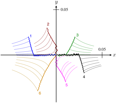
Figure 3: Illustration of different policies learned after starting from six different locations: $\boldsymbol{x}_{1}=[-0.03,0.02]$, $\boldsymbol{x}_{2}=[-0.01,0.03]$, $\boldsymbol{x}_{3}=[0.02,0.02]$, $\boldsymbol{x}_{4}=[0.03,-0.02]$, $\boldsymbol{x}_{5}=[0.01,-0.03]$, $\boldsymbol{x}_{6}=[-0.02,-0.04]$. The learning parameters are $\alpha=\beta=10$, $N=4$, $\gamma=0.95$ and $p=1$. In each case we use as many batches as required to get the final position of the drop below $0.0015$. We plot the resulting policy in thick solid, while the thin lines show what the drop would do in the absence of speed control.

We next illustrate how the algorithm performs from different starting points, as well as how trajectories change depending on the initial position. We again take $\alpha=\beta=10$, $N=4$, $\gamma=0.95$, $p=1$ and choose the same time parameters as before. We consider six different starting points $\boldsymbol{x}_{k}$ located in the four quadrants, specifically $\boldsymbol{x}_{1}=[-0.03,0.02]$, $\boldsymbol{x}_{2}=[-0.01,0.03]$, $\boldsymbol{x}_{3}=[0.02,0.02]$, $\boldsymbol{x}_{4}=[0.03,-0.02]$, $\boldsymbol{x}_{5}=[0.01,-0.03]$, $\boldsymbol{x}_{6}=[-0.02,-0.04]$. The algorithm trains for each point separately, i.e. it computes a different policy for each value of $\boldsymbol{x}_{k}$. For each starting point, we allow the algorithm to practice on as many batches as needed until $\overline{|\boldsymbol{x}_{\text{f}}|}$ drops below $0.0015$. This never took more than $7$ batches, i.e. $700$ episodes.

We show in Fig. 3 the trajectories resulting from the learned policies (to reduce crowding, each trajectory terminates as soon as the distance from the origin at the end of a time step becomes smaller than $0.002$). In each case, the controlled motion of the drop is shown in thick solid, while the thins lines correspond to the paths that the drop would follow if it were not for speed control (these paths coincide with the streamlines in Fig. 1). In all cases, we see that the algorithm succeeds in bringing the drop back to the origin. All trajectories present small diagonal drifts caused by bursts of increased rotation, separated by free motion along the streamlines. Computationally, points further away from the origin required more training; for example, finding the trajectory starting from $\boldsymbol{x}_{3}$ in Fig. 3 only required $200$ training runs, while the one starting from $\boldsymbol{x}_{4}$ took $700$.

We close by emphasising that, in all cases illustrated in Fig. 3, the policy is different for each starting point; in §VII we investigate whether it is possible to find a global policy that is effective for all starting points.

VI Learning process and parameters

The previous section demonstrated the effectiveness of Reinforcement Learning in controlling the motion of the drop. We now investigate how accuracy and learning speed depend on the various parameters used by the algorithm. Then we examine in §VII how the algorithm deals with noise and with finding a global policy. As explained in §IV, learning is assessed by running a fixed number of batches ($n_{\text{batches}}$) of $100$ episodes and plotting the values of the average final distance $\overline{|{\boldsymbol{x}}_{f}|}$ in each batch. Since results are random, we quantify the uncertainty in each learning curve $\overline{|{\boldsymbol{x}}_{f}|}_{i}$ ($1\leq i\leq n_{\text{batches}}$) by generating it twice with the same parameters and returning the average relative error

$$\Delta=\frac{1}{n_{\text{batches}}}\sum_{i=1}^{n_{\text{batches}}}\frac{\left|\overline{|{\boldsymbol{x}}_{f}|}_{i}^{(1)}-\overline{|{\boldsymbol{x}}_{f}|}_{i}^{(2)}\right|}{\overline{|{\boldsymbol{x}}_{f}|}_{i}^{(1)}}.$$ (27)

Since the setup is four-fold symmetric, we restrict our attention to the case where the drop starts out in the second quadrant (denoted by $11$, see Fig. 2).

VI.1 Varying the discount Factor $\gamma$

We start by setting $p=1$, $\alpha=\beta=5$, $N=4$, $t_{\text{max}}=40$ and aim to find the value of the discount factor $\gamma$ which causes $\overline{|\boldsymbol{x}_{\text{f}}|}$ to decrease the fastest. We ignore the values $\gamma=0$ and $\gamma=1$, since $\gamma=0$ would result in a very shallow one-step lookahead, and $\gamma=1$ would not ensure $\gamma^{t_{\text{max}}}\approx 0$, while decay is required in the updates of the Actor-Critic method. In Fig. 4 we plot the average final distance $\overline{|\boldsymbol{x}_{\text{f}}|}$ as a function of the batch number for different values of $\gamma$ in the range $(0,1)$. Clearly performance improves steadily with $\gamma$, showing that we can base our choice of actions on long-term predictions; the larger the value of $\gamma$ the more we penalize bad actions far ahead in the future, since the $k$th reward gets discounted by $\gamma^{k-1}$. The average relative errors are small, indicating that the variance within each learning curve is likely to be small. Since it gave the best performance, we take $\gamma=0.95$ in what follows.

Figure 4: Average final distance of the drop from the stagnation point, $\overline{|\boldsymbol{x}_{\text{f}}|}$, as a function of the batch number for different values of the discount factor, $\gamma$ (see text for the values of the other parameters).

VI.2 Varying the peakedness $p$ of the reward function

Figure 5: Average final distance of the drop from the stagnation point, $\overline{|\boldsymbol{x}_{\text{f}}|}$, as a function of the batch number for different values of peakedness $p$ of the reward function (see text for the values of the other parameters).

To address the impact of the peakedness $p$ of the reward function, in Fig. 5 we plot the learning curves obtained by running the algorithm with the values $\alpha=\beta=5$, $N=4$, $t_{\text{max}}=40$, $\gamma=0.95$ and different values of $p$. Small values of $p$, such as $p=0.01$, do not adequately discriminate between actions, while very large values (e.g. $p=10$) hinder exploration by treating all bad actions as equally undesirable, and also take longer to run. The average relative errors are again very small, which makes us confident that the displayed curves are representative samples. Within a small window from $p=0.5$ to $p=1.5$, the learning speed increases slightly, but since results are all very similar we keep $p=1$ in what follows.

VI.3 Varying the gradient ascent parameters $\alpha$, $\beta$

Even with the previous choices of parameters, it still takes approximately $1000$ episodes to reach a final accuracy of $\overline{|\boldsymbol{x}_{\text{f}}|}=0.005$ ($10$ batches of $100$ episodes, or more). Out of all parameters, we found that the gradient ascent parameters $\alpha$ and $\beta$ have the biggest impact on learning speeds. When chosen correctly, they can reduce the number of training episodes to just a few hundred. To demonstrate this, we take $t_{\text{max}}=40$, $N=4$, $p=1$, $\gamma=0.95$ and monitor the final average distance $\overline{|\boldsymbol{x}_{\text{f}}|}$ for various values of $\alpha=\beta$; the resulting learning curves are shown in Fig. 6. Performance increases steadily with $\alpha=\beta$. The values $\alpha=\beta=10$ lead to a steep learning curve, dropping below $0.01$ after only $3$ iterations. The only real constraint on these parameters is that they cannot be arbitrarily large, because for $\gamma=0.95$ the Actor-Critic algorithm may give very large entries for $\boldsymbol{C}$ and $\boldsymbol{D}$, making it hard to find a suitable $B$ for the rejection sampling part (§III.8). Furthermore, the final gradient ascent update in each episode has size $\mathcal{O}(\gamma^{t_{\text{max}}}\alpha)$. If we want this to be reasonably small for $t_{\text{max}}=40$ and $\gamma=0.95$, e.g. less than $1$, we should take $\alpha\lesssim 8$. As in the previous simulations, the relative errors are seen to be very small. We therefore settle on the values $\alpha=\beta=10$ in what follows.

Figure 6: Average final distance of the drop from the origin, $\overline{|\boldsymbol{x}_{\text{f}}|}$, as a function of the batch number for different values of the gradient ascent parameters $\alpha=\beta$ (see text for the values of the other parameters).

VI.4 Varying the size $N$ of policy and value function arrays

We next examine the impact of the size $N$ of the policy and value function arrays ${\boldsymbol{C}}$ and ${\boldsymbol{D}}$. To see how this parameter affects the final accuracy and the learning speed, we choose $5$ different values of $N$ and run $10$ batches for each value (the other parameters are kept at $t_{\text{max}}=40$, $p=1$ and $\alpha=\beta=10$, $\gamma=0.95$). The learning curves are displayed in Fig. 7. We see that the choice $N=1$ performs poorly since $\hat{\pi}$ becomes a uniform distribution; the remaining values give very similar results, with small relative errors $\Delta$, so we keep $N=4$ in what follows.

Figure 7: Average final distance of the drop from the origin, $\overline{|\boldsymbol{x}_{\text{f}}|}$, as a function of the batch number for different values of the array size $N$ (see text for the values of the other parameters).

VI.5 Varying the step size $dt$ and the length of episodes $t_{\text{max}}$

The accuracy of the algorithm depends strongly on the step size $dt$, with larger values leading to a poorer accuracy. Furthermore, for large values of $dt$, learning may still occur but the learning curve is no longer steadily decreasing with batch number because bad actions can take the drop further away from the target. Through extensive simulations, we found empirically that $dt$ should be chosen so that the particle can never move by a distance larger than the desired final accuracy during a time step. In their original paper, Bentley and Leal state that a dimensionless final distance of $0.0078$ is enough for their experiments  (bentley1986computer, ), and since $\overline{|\boldsymbol{x}_{\text{f}}|}$ was consistently below this threshold in the previous sections, our chosen $dt$ is sufficiently small.

The length of the episodes $t_{\text{max}}$ is also an important parameter. To investigate how it affects performance, we fix the values $N=4$, $\alpha=\beta=10$, $\gamma=0.95$, $p=1$ and monitor how the learning speed depends on $t_{\text{max}}$ when it is equal to $40$, $50$, $80$, $100$. For each value, we run $10$ batches of episodes of $t_{\text{max}}$ steps each, until we reach a total of $40,000$ steps. This way, all batches consist of $4000$ time steps and we can compare learning speed batch by batch. The sizes of our batches are thus, respectively, $100$, $80$, $50$ and $40$. The resulting learning curves are shown in Fig. 8. The learning curve seems to get steeper as $t_{\text{max}}$ increases, signifying that the algorithm takes longer to identify the optimal strategy. A possible explanation for this result is as follows. Since $\gamma$ is very close to $1$, there is very little discounting in the first few time steps. Therefore, if $t_{\text{max}}$ is large, the algorithm can afford to pick sub-optimal actions in the beginning because it has time to recover. Conversely, if $t_{\text{max}}$ is small the algorithm cannot waste time on bad actions and needs to aim for the target from the start. After the initial phase, the algorithm proved more accurate for larger values of $t_{\text{max}}$, likely because the drop is allowed to explore the environment for longer. All learning curves consistently plateau around the $\overline{|\boldsymbol{x}_{\text{f}}|}=0.001$ mark and relative errors are small. For the purpose of the experiments in Ref. (bentley1986computer, ), performance is essentially the same in all four case, so we keep $t_{\text{max}}=40$, which had the smallest $\Delta$.

Figure 8: Average final distance of the drop from the stagnation point, $\overline{|\boldsymbol{x}_{\text{f}}|}$, as a function of the batch number for different values of the length of episodes $t_{\text{max}}$ (see text for the values of the other parameters).

VI.6 Varying the rotation wiggle rooms

As a reminder, the wiggle room $w$ is the half-width of the window of (dimensionless) angular velocity within which the cylinders are allowed to change their speeds. This is another important parameter that affects learning speed. If the initial position $\boldsymbol{x}_{0}$ is far from the origin, large changes in the fluid velocity, and therefore in the torques, may be needed to prevent the drop from wandering out of the state space.

To illustrate this, Fig. 9 shows the learning curves obtained from $\boldsymbol{x}_{0}$ (with $\alpha=\beta=10$, $p=1$, $\gamma=0.95$, $t_{\text{max}}=40$, $N=4$) when the wiggle rooms are $w=0.5$, $0.6$, $0.7$ and $0.8$. We see that errors are almost always negligible and that even a small difference in the the allowed rotations significantly affects the learning speed; small wiggle rooms mean that we need to be more precise with our choice of actions, because we may not be able to recover from a bad one.

Figure 9: Average final distance of the drop from the origin, $\overline{|\boldsymbol{x}_{\text{f}}|}$, as a function of the the batch number for four different rotation wiggle rooms $w$ (see text for the values of the other parameters).

From a practical standpoint, a small wiggle room might be preferable to prevent high torques and accelerations of the cylinders. However, a value that is too small prevents the algorithm from stabilising the drop. In general, points further away from the origin will require bigger leeways, and reducing the wiggle rooms decreases learning performance. We keep our wiggle rooms at $w=0.7$, which gave good performance while in general requiring less torque than $w=0.8$.

VI.7 Variance

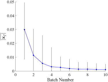
Figure 10: Variance and improvement during learning: Average final distance of the drop from the origin $\overline{|\boldsymbol{x}_{\text{f}}|}$ and range of distances as a function of the the batch number (see text for the values of the learning parameters).

After running a batch, we used the resulting policy to simulate $100$ episodes in order to estimate the average final distance $\overline{|\boldsymbol{x}_{\text{f}}|}$. Let $X_{i}$ be the final distance from the origin in the $i$-th episode. In order for the algorithm to be useful in practice we need consistency, i.e. for $\max(X_{i})$ to be as small as possible. To test this, we run $10$ batches with the parameters $N=4$, $\alpha=\beta=10$, $\gamma=0.95$, $p=1$ and $t_{\text{max}}=40$. For each batch, in Fig. 10 we plot $\overline{|\boldsymbol{x}_{\text{f}}|}$ along with the range of the corresponding $X_{i}$. We can see that the algorithm is initially rather inaccurate, but then slowly improves and becomes more consistent. In batch $10$, all episodes land within $0.0051$ of the origin, which is smaller than the (dimensionless) distance required for the experiments of Ref. (bentley1986computer, ).

In order to better understand the distribution of $X_{i}$, Fig. 11 shows the approximate CDF obtained in the last batch. The distribution is clearly skewed towards $x=0$, with only $3\%$ of the $X_{i}$ lying in $x>0.002$.

VII Robustness of the learned policy and further control

So far we have established the effectiveness of our Reinforcement Learning algorithm in stabilising the drop trajectory when the algorithm is trained against deterministic motion and when the drop always starts at a fixed location in space. In this section we relax these two assumptions. First we establish that the policy learned in the absence of noise continues to work even in the presence of thermal noise (§VII.1). We next study the extent to which the policy learned from a given starting point is effective when the drop starts from another location (§VII.2). Finally, motivated by experiments where the drop is stretched by the flow in a controlled way, we propose a variant of the algorithm designed to control the extension rate of the flow at the location of the flow (§VII.3).

Figure 11: Cumulative distribution function (CDF) of the distance of the drop from the origin after $1,000$ episodes (i.e. in batch 10; see text for the values of the learning parameters).

VII.1 Noise

The dynamics of the drop so far followed Eq. (4) with the model flow from Eq. (1) and it was therefore fully deterministic. Motivated by experimental situations where the drop is small enough to be impacted by thermal noise, we now examine the performance of the deterministic Reinforcement Learning algorithm in a noisy situation.

We incorporate thermal noise using a Langevin approach batchelor1976 . In a dimensional setting, this is classically done by adding a random term $M\boldsymbol{F}$ to Eq. (4) where $M=(6\pi\mu r)^{-1}$ is the mobility of the spherical drop in a fluid of viscosity $\mu$ and $\boldsymbol{F}$ is a random force. We assume that $\boldsymbol{F}$ has zero mean value (i.e. $\langle F_{i}(t)\rangle=0$, where we use $\langle\rangle$ to denote ensemble averaging) and that it satisfies the fluctuation-dissipation theorem

$$\langle F_{i}(t)F_{j}(t^{\prime})\rangle=\frac{2k_{B}T}{M}\delta_{ij}\delta(t-t^{\prime}),$$ (28)

where $k_{B}=1.3806\times 10^{-23}~{}J\text{K}^{-1}$ is Boltzmann’s constant and $T$ is the absolute temperature.

Moving to dimensionless variables, we used the half distance between the cylinders, $L$, as the characteristic length scale and the inverse cylinder rotation speed, $\tau$, as the characteristic time scale (see §IV.2), so Eq. (28) allows to define a typical magnitude for the random force, given by $F_{0}=(k_{B}T/M\tau)^{1/2}$. Non-dimensionalising $F$ by $F_{0}$, the Langevin approach consists then in adding a random term of the form ${\rm Pe}^{-1/2}\tilde{F}$ to the dimensionless version of Eq. (4), where $\tilde{F}$ is a dimensionless random force with $\langle\tilde{F}_{i}\rangle=0$ and $\langle\tilde{F}_{i}(t)\tilde{F}_{j}(t^{\prime})\rangle=2\delta_{ij}\delta(t-t^{\prime})$. Here ${\rm Pe}$ is the dimensionless Péclet number, which compares the relative magnitude of advection by the flow and Brownian diffusion

$${\rm Pe}\equiv\frac{L^{2}}{\tau k_{B}TM}.$$ (29)

We implement the Langevin approach numerically by adding a random term $\left({2\Delta t}/{\text{Pe}}\right)^{1/2}\Gamma_{i}$ at the end of each numerical step, where $\Delta t$ is the step size used in the RK4 scheme and $\Gamma_{i}$ ($i=1,2$) is drawn from a standard normal distribution.

Physically, the Péclet number in Eq. (29) can be recast as a ratio between the radius of the drop $r$ and a thermal length scale $\ell$,

$${\rm Pe}=\frac{r}{\ell}\quad\ell\equiv\frac{\tau k_{B}T}{6\pi\mu L^{2}}.$$ (30)

With the dimensions from §IV.2, we have $L={6.35\times 10^{-2}}$ m, $\tau=8$ s, and assuming the fluid to be water at room temperature ($T=293$ K, viscosity $\mu=10^{-3}$ Pas), we obtain $\ell\approx 4.3\times 10^{-16}$ m. In the original work from Ref. bentley1986experimental , the typical drop has radius $r\approx 0.5$ mm, which leads to ${\rm Pe}\approx{1.2\times 10^{12}}$ in these experiments. This very large number clearly indicates that thermal noise was not important in this original work.

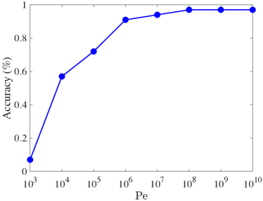
Figure 12: Proportion of episodes landing within a dimensionless distance $0.0078$ of the origin for different values of the Péclet number (${\rm Pe}$) using the algorithm trained in the absence of noise (see text for the values of the learning parameters). The original experiments in Ref. bentley1986experimental had ${\rm Pe}\approx{1.2\times 10^{12}}$.

To test robustness, we applied the policy obtained via the Reinforcement Learning algorithm from the previous sections (i.e. under deterministic drop dynamics) to environments with progressively smaller values of the Péclet number, which corresponds physically to shrinking the scale of the drop so that thermal noise becomes progressively more important. The parameters of the algorithm are once again $\alpha=\beta=10$, $N=4$, $\gamma=0.95$, $p=1$, $dt=0.025$, $t_{\rm lag}=0.0125$, $t_{1}=t_{2}=0.005$ and $t_{\text{max}}=40$; the wiggle rooms are set to $w=0.7$. After $500$ training runs, we let Pe take values $\mathrm{Pe}=10^{k}$, $3\leq k\leq 8$, and simulated $100$ separate episodes in each case. Fig. 12 shows the corresponding proportions of runs landing within a distance $0.0078$ of the origin. As expected, the accuracy decreases when the Pe number becomes smaller, dropping from a largest value of $0.97$ when Pe${\rm Pe}=10^{10}$ to $0.07$ when ${\rm Pe}=10^{3}$. The algorithm was more than $90\%$ accurate for Pe $\geq 10^{6}$, which is six orders of magnitude smaller than in Bentley and Leal’s experiment (and thus would correspond to nanometer-sized drops). It is worth mentioning that, even though we did not do it in this work, noise could be included in the training phase rather than added once the policy has been found.

VII.2 Global Policy

So far the learned policy was always obtained for the same fixed starting point ${\boldsymbol{x}}_{0}$. Can we, on the other hand, obtain a policy that is optimal (or sufficiently close to optimal) for all starting point? Intuitively, points in the state space that are close together should have similar optimal policies, so if the state space itself is sufficiently small such a global policy should exist. Should this not be the case, we would have to split the state space in smaller regions and to determine a globally good policy in each region separately.

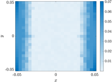
Figure 13: Final distances from the origin for $625$ trajectories starting in the $[-0.05,0.05]\times[-0.05,0.05]$ space using the optimal policy $\pi_{*}$ obtained from the single dimensionless starting position ${\boldsymbol{x}}_{0}=[-0.03,0.02]$. The time and learning parameters $dt=0.025$, $t_{\rm lag}=0.0125$, $t_{1}=t_{2}=0.005$, $\gamma=0.95$, $p=1$, $\alpha=\beta=10$, $N=4$, $t_{\text{max}}=40$.

We investigate the existence of a global policy by estimating the optimal policy $\pi_{*}$ from the dimensionless starting position ${\boldsymbol{x}}_{0}=[-0.03,0.02]$ and then running trajectories from a number of other points in the state space. We use the time and learning parameters $dt=0.025$, $t_{\rm lag}=0.0125$, $t_{1}=t_{2}=0.005$, $\gamma=0.95$, $p=1$, $\alpha=\beta=10$, $N=4$, $t_{\text{max}}=40$. After $500$ training runs in a noiseless environment, we construct a $25\times 25$ rectangular lattice of evenly spaced points in the state space $[-0.05,0.05]\times[-0.05,0.05]$ and run a trajectory from each one of them using the policy obtained for $\boldsymbol{x}_{0}$ (i.e. no further learning occurs during that process). We then use the results to build a colour map of the final distances, i.e. a $25\times 25$ matrix $M$ where $M_{ij}$ is coloured according to the final distance from the origin of a trajectory starting from the corresponding location on the grid. We show the results for all $625$ trajectories in the absence of thermal noise in Fig. 13. We can see that all unsuccessful starting points are clustered around the edge of the state space on the sides where the flow points away from the origin, suggesting that we can indeed find a global policy by making the state space a bit smaller. The algorithm was successful in $61.12\%$ of cases, with an average final distance of $0.0160$ and a standard deviation of $0.0213$. The average final distance is heavily skewed by the edge cases. In the region $[-0.03,0.03]\times[-0.05,0.05]$, corresponding the lighter strip in the middle, the average final distance was $0.0012$ with a standard deviation of $7.7026\times 10^{-4}$ and a success rate of $100\%$. The largest final distance in this region was $0.0075$ and the smallest was $6.1237\times 10^{-5}$. To see how thermal noise affects this result, we carry out the same simulations by incorporating noise as in §VII.1 in the case where ${\rm Pe}=10^{5}$, with results shown in Fig. 14. The algorithm was now successful in $60.96\%$ of cases, with an average final distance of $0.0164$ ad a standard deviation of $0.0209$. Again, if we restrict the set of initial states to those in $[-0.03,0.03]\times[-0.05,0.05]$ these figures improve significantly. Success rate jumps to $97.07\%$ and the average final distance becomes $0.0019$ with a standard deviation of $0.0020$. The largest final distance in this region was $0.0153$ and the smallest was $1.4041\times 10^{-4}$. In summary, the overall performance was quite similar to the noiseless case, except for a small decrease in accuracy and consistency in the central region. This shows that the algorithm is robust to noise even in the case of nanometer-sized drops.

Figure 14: Same as Fig. 13 in the case where thermal noise is added to the drop trajectory with ${\rm Pe}=10^{5}$.

VII.3 Extension Rate Control

Returning to the physical aspects of the experiment, Taylor’s original study addressed how the properties of the flow affected the shape of the drop taylor1934formation . When the drop is fixed at the origin, its rate of deformation is dictated by the eigenvalues of the velocity gradient tensor, $\nabla\boldsymbol{u}(\boldsymbol{0})$. The flows considered in this study are two-dimensional and irrotational so that $\nabla\boldsymbol{u}$ remains symmetric and traceless throughout. The velocity gradient is thus characterised by a pair of eigenvalues $\lambda_{0}>0$ (extension rate) and $-\lambda_{0}<$ (compression). When we alter the speeds of the cylinder with the control algorithm, we inevitably change the eigenvalues of $\nabla\boldsymbol{u}(\boldsymbol{x})$, where $\boldsymbol{x}$ is the position of the drop, leading to a time-dependent eigenvalue $\lambda(t)$. Since this eigenvalue controls the deformation of the drop, we wish to keep its magnitude as close as possible to the extension rate $\lambda_{0}$ which we aim to study while we control the drop position.

Here we examine the case where the starting position is $\boldsymbol{x}_{0}=[-0.03,0.02]$, with the same parameters as above (i.e. $dt=0.025$, $t_{\rm lag}=0.0125$, $dt=t_{1}=t_{2}=0.005$, $\gamma=0.95$, $p=1$, $\alpha=\beta=10$, $N=4$, $t_{\text{max}}=40$). We assume the drop is subject to thermal noise with ${\rm Pe}=10^{5}$. After $500$ training runs, we simulate a $40$-step trajectory (in which no learning occurs) during which we sample the extension rate $20$ times per time step. In Fig. 15A we plot the variation of the scaled extension rate, $\lambda(t)/\lambda_{0}$, with time, where $\lambda_{0}$ is the value at the centre of the uncontrolled apparatus (using the dimensionless parameters in the problem, we have $\lambda_{0}=1.28$). The extension rate is seen to undergo significant variations during the controlled motion of the drop, with jumps that are routinely $\pm 15\%$ about the desired value $\lambda_{0}$. The norm of the final state was $0.0056$.

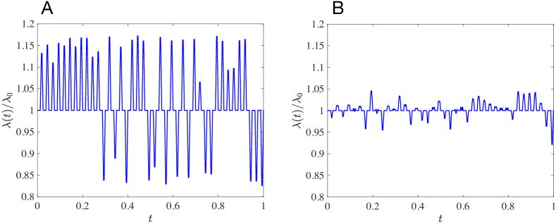
Figure 15: Ratio between the extension rate $\lambda(t)$ and the reference value $\lambda_{0}$ at the centre of the uncontrolled apparatus. A: Without scaling, the extension rate routinely varies by $15\%$ around $\lambda_{0}$. B: Using the piecewise linear scaling from Eq. (31), the fluctuations of the extension rate near the drop are significantly reduced. The time and learning parameters are $dt=0.025$, $t_{\rm lag}=0.0125$, $dt=t_{1}=t_{2}=0.005$, $\gamma=0.95$, $p=1$, $\alpha=\beta=10$, $N=4$, $t_{\text{max}}=40$ while the Péclet number is ${\rm Pe}=10^{5}$.

To lower the variations on $\lambda(t)$ and keep it closer to its target value, we modified the algorithm as follows. The idea is to note that if an angular velocity vector $\boldsymbol{\Omega}$ (i.e. the vector of all four cylinder rotations) induces an extension rate $\lambda$ at $\boldsymbol{x}$, then by linearity the angular velocity vector $k\boldsymbol{\Omega}$ induces an extension rate $k\lambda$ at the same point ($k\in\mathbb{R}$). We may then scale, at each time step, $\boldsymbol{\Omega}$ with a suitable scalar function $s(t)$ so that the angular velocity vector changes as $s(t)\cdot\boldsymbol{\Omega}(t)$, where $\boldsymbol{\Omega}(t)$ corresponds to standard speed modulation. Since the jumps in $\lambda(t)$ are due to the rapid changes in angular velocities, we choose $s(t)$ to minimize the impact of speed modulation. Specifically, at time step $t_{k}$ and state $\boldsymbol{x}_{k}$ we denote $\Lambda=\lambda_{0}/\hat{\lambda}$, where $\hat{\lambda}$ is the extension rate at $\boldsymbol{x}_{k}$ resulting from unscaled speed modulation. Then we take a piece-wise linear scaling

$$s(t)=\begin{cases}1,\,t_{k}\leq t\leq t_{k}+t_{\rm lag},\\ \left|(\Lambda-1)\frac{t-(t_{k}+t_{\rm lag})}{\delta}+1\right|,\,0\leq t-(t_{k}+t_{\rm lag})\leq\delta,\\ \Lambda\ \ \ \text{ if }t_{\rm lag}+\delta\leq t-t_{k}\leq dt-\delta,\\ \left|(1-\Lambda)\frac{t-(t_{k}+dt)+\delta}{\delta}+\Lambda\right|,\,-\delta\leq t-(t_{k}+dt)\leq 0,\end{cases}$$ (31)

and choose $\delta=t_{1}=t_{2}$. To compensate for this scaling, we also make the change $dt\to dt/\Lambda$. In Fig. 15B we show the evolution of the extension rate (scaled by $\lambda_{0}$) in a trajectory with the same parameters as before but with our scaling implemented. A couple of large excursions remain, but performance has noticeably improved relative to the original control algorithm (left). The norm of the final state was $9.4389\times 10^{-4}$, indicating that scaling does not affect accuracy. This proof-of-principle result shows therefore that a scaling in the optimal policy can be used to limit the extension rate in the flow.

VIII Discussion

In this paper we saw how Reinforcement Learning can be applied to solve a classical control problem for fluid dynamics at low Reynolds numbers. Our goal here was to modulate the rotation speeds of a model of Taylor’s four-roll mill in order to stabilize a drop positioned near the stagnation point, which is known to be unstable. We implemented an Actor-Critic method and found a probabilistic policy that worked well for all initial positions.

In our approach, we proceeded by steps. We first derived a basic version of the algorithm, and then added measurement delays, thermal noise and extension rate control. The algorithm was able to manoeuvre the drop effectively in all cases and the accuracy achieved was below that required in the experiments of Bentley and Leal bentley1986experimental , and therefore satisfactory for most experimental implementations. Numerical results shown in §VI also demonstrated that learning is remarkably consistent, with minimal variance within the learning curves in the majority of cases.

The good performance observed was, to a large extent, due to our choice of actions rather than to the quality of the approximation for the policy ($\pi$). Indeed, numerical results in Fig. 7 show that a first order approximation of the form $\pi\approx K\exp(ax+by)$ is sufficient to get accurate results. In practice, the learning process was often slower at the beginning, when the algorithm had not yet gathered enough information to take good actions. Then, once the general shape of the policy had been identified, learning sped up significantly, until it slowly tapered off as we approached the theoretical accuracy.

It is worth mentioning here that we attempted other implementations too, which were not successful . We initially tried to discretize the state space, so that the drop would move in a finite grid as opposed to a continuous environment, but it was difficult to combine this with the Markov property and harder to factor in thermal noise. We also used a truncated Fourier series for the form of the function $f$, but this was computationally expensive and it artificially introduced discontinuities as well as Gibbs’ phenomena.

Finally, we also experimented with the shape of the reward function, seeking to penalise actions requiring very large torques. Unfortunately, our attempted modifications in that regard (such as subtracting some simple increasing function of the torque from $R_{t}$) did not succeed. After extensive simulations, we concluded that torque reduction can be achieved by either shrinking the sate space (so that smaller corrections are needed) or reducing the default angular velocities.

There are many possible extensions to our work. One could try an algorithm with higher sample efficiency (i.e. one which makes better use of past experience), one that better balances exploration and exploitation, or a different learning paradigm altogether (i.e. a neural network). We may also implement different approximations for the value function as well as alternative rewards and sampling methods. It would also be interesting to devise a model where time is continuous.

From a physical standpoint, it might be desirable to include inertia (both of the drop and the fluid) and include a nonzero response time to variations in $\boldsymbol{\Omega}$. We could also allow ourselves to act on more than one cylinder at a time or to undo an action by exploiting the time-reversibility of the viscous flow. Another area for improvement is extension rate control, since some jumps in Fig. 15 still remain. Finally, one could devise a model where one only has incomplete knowledge of the drop’s position.

Supplementary Material

We include in Supplementary Material SM a movie of the trajectory displayed in Fig. 2. In the movie, the histogram on the left shows the current angular velocity of each cylinder, as well as their average value. The diagram on the right shows the motion of the drop inside the state space as well as the rotation of each cylinder (note that the radii of both the drop and the cylinders are not to scale) and the eigenvectors of $\nabla{\bf u}$ at the location of the drop (note that since the flow is irrotational, these are also the eigenvectors of the rate-of-strain tensor). For clarity, the cylinders are displayed on the corners of the state space, rather than in their actual locations.

Matlab code

The code created in this work is freely available as a matlab .m file on GitHub GH . To estimate the optimal policy, the user needs to initialize the parameters, add a section break as indicated and run as many batches (outer "for" loops) as needed. The parameter AverageDistance corresponds to the average final distance for the current batch, and can be used to assess performance. By commenting out lines $76-82$ in the code, the program can be used to simulate trajectories during which no learning occurs.

Appendix A Proof of rejection sampling algorithm

We need to show that the conditional distribution of $X$ is $p$. Let $P$ be the cumulative distribution function of $p$ and $Q$ that of $q$. Then by Bayes theorem

$$\mathbb{P}\left(X\leq x|Y\leq\alpha\right)=\frac{\mathbb{P}\left(Y\leq\alpha|X\leq x\right)Q(x)}{\mathbb{P}(Y\leq\alpha)}$$ (32)

$$\mathbb{P}\left(Y\leq\alpha|X\leq x\right) =\frac{\mathbb{P}\left(Y\leq\alpha,X\leq x\right)}{Q(x)}$$ (33)

$$=\int^{x}\frac{\mathbb{P}(Y\leq\alpha|X=t)}{Q(x)}q(t)\mathrm{d}t$$ (34)

$$=\frac{1}{Q(x)}\int^{x}\frac{A\cdot p(t)}{B\cdot q(t)}q(t)\mathrm{d}t$$ (35)

$$=\frac{A\cdot P(x)}{B\cdot Q(x)}$$ (36)

Also

$$\mathbb{P}(Y\leq\alpha)=\int_{I}\frac{A\cdot p(t)}{B\cdot q(t)}q(t)\mathrm{d}t=\frac{A}{B}$$ (37)

Substituting, we see that $\mathbb{P}\left(X\leq x|Y\leq\alpha\right)=P(x)$, so, conditional on being accepted, $X\sim p$.

References

- [1] G. I. Taylor. The formation of emulsions in definable fields of flow. Proc. Roy. Soc. A, 146:501–523, 1934.
- [2] J. J. L. Higdon. The kinematics of the four-roll mill. Phys. Fluids, 5:274–276, 1993.
- [3] B. J. Bentley and L. G. Leal. An experimental investigation of drop deformation and breakup in steady, two-dimensional linear flows. J. Fluid Mech., 167:241–283, 1986.
- [4] J. Eggers. Nonlinear dynamics and breakup of free-surface flows. Rev. Mod. Phys., 69:865–929, 1997.
- [5] J. M. Rallison. The deformation of small viscous drops and bubbles in shear flows. Annu. Rev. Fluid Mech., 16:45–66, 1984.
- [6] H. A. Stone, A. D. Stroock, and A. Ajdari. Engineering flows in small devices: microfluidics toward a lab-on-a-chip. Annu. Rev. Fluid Mech., 36:381–411, 2004.
- [7] T. M. Squires and S. R. Quake. Microfluidics: Fluid physics at the nanoliter scale. Rev. Mod. Phys., 77:977–1026, 2005.
- [8] S. D. Hudson, F. R. Phelan Jr, M.D. Handler, J. T. Cabral, K. B. Migler, and E. J. Amis. Microfluidic analog of the four-roll mill. Appl. Phys. Lett., 85:335–337, 2004.
- [9] J. S. Lee, R. Dylla-Spears, N. P. Teclemariam, and S. J. Muller. Microfluidic four-roll mill for all flow types. Appl. Phys. Lett., 90:074103, 2007.
- [10] M. Tanyeri, E. M. Johnson-Chavarria, and C. M. Schroeder. Hydrodynamic trap for single particles and cells. Appl. Phys. Lett., 96:224101, 2010.
- [11] M. Tanyeri, M. Ranka, N. Sittipolkul, and C. M. Schroeder. A microfluidic-based hydrodynamic trap: design and implementation. Lab Chip, 11:1786–1794, 2011.
- [12] A. Shenoy, C. V. Rao, and C. M. Schroeder. Stokes trap for multiplexed particle manipulation and assembly using fluidics. Proc. Natl. Acad. Sci. USA, 113:3976–3981, 2016.
- [13] B. J. Bentley and L. G. Leal. A computer-controlled four-roll mill for investigations of particle and drop dynamics in two-dimensional linear shear flows. J. Fluid Mech., 167:219–240, 1986.
- [14] R. S. Sutton and A. G. Barto. Reinforcement learning: An introduction. MIT press, 2018.
- [15] M. P. Brenner, J. D. Eldredge, and J. B. Freund. Perspective on machine learning for advancing fluid mechanics. Phys. Rev. Fluids, 4:100501, 2019.
- [16] S. L. Brunton, B. R. Noack, and P. Koumoutsakos. Machine learning for fluid mechanics. Annu. Rev. Fluid Mech., 52:477–508, 2020.
- [17] F. Guéniat, L. Mathelin, and M. Y. Hussaini. A statistical learning strategy for closed-loop control of fluid flows. Theor. Comp. Fluid Dyn., 30:497–510, 2016.
- [18] J. Rabault, M. Kuchta, A. Jensen, U. Réglade, and N. Cerardi. Artificial neural networks trained through deep reinforcement learning discover control strategies for active flow control. J. Fluid Mech., 865:281–302, 2019.
- [19] Y. Xie and X. Zhao. Sloshing suppression with active controlled baffles through deep reinforcement learning–expert demonstrations–behavior cloning process. Phys. Fluids, 33:017115, 2021.
- [20] V. Belus, J. Rabault, J. Viquerat, Z. Che, E. Hachem, and U. Reglade. Exploiting locality and translational invariance to design effective deep reinforcement learning control of the 1-dimensional unstable falling liquid film. AIP Advances, 9:125014, 2019.
- [21] J. Viquerat, J. Rabault, A. Kuhnle, H. Ghraieb, A. Larcher, and E. Hachem. Direct shape optimization through deep reinforcement learning. J. Comp. Phys., 428:110080, 2021.
- [22] G. Novati, H. L. de Laroussilhe, and P. Koumoutsakos. Automating turbulence modelling by multi-agent reinforcement learning. Nature Mach. Int., 3:87–96, 2021.
- [23] R. Paris, S. Beneddine, and J. Dandois. Robust flow control and optimal sensor placement using deep reinforcement learning. J. Fluid Mech., 913:A25, 2021.
- [24] M. Gazzola, A. A. Tchieu, D. Alexeev, A. de Brauer, and P. Koumoutsakos. Learning to school in the presence of hydrodynamic interactions. J. Fluid Mech., 789:726–749, 2016.
- [25] G. Novati, S. Verma, D. Alexeev, D. Rossinelli, W.M. Van Rees, and P. Koumoutsakos. Synchronisation through learning for two self-propelled swimmers. Bioinsp. Biomim., 12:036001, 2017.
- [26] S. Verma, G. Novati, and P. Koumoutsakos. Efficient collective swimming by harnessing vortices through deep reinforcement learning. Proc. Natl. Acad. Sci. USA, 115:5849–5854, 2018.
- [27] G. Novati, L. Mahadevan, and P. Koumoutsakos. Controlled gliding and perching through deep-reinforcement-learning. Phys. Rev. Fluids, 4:093902, 2019.
- [28] Y. Jiao, F. Ling, S. Heydari, E. Kanso, N. Heess, and J. Merel. Learning to swim in potential flow. Phys. Rev. Fluids, 6:050505, 2021.
- [29] D. Fan, L. Yang, Z. Wang, M. S. Triantafyllou, and G. E. Karniadakis. Reinforcement learning for bluff body active flow control in experiments and simulations. Proc. Natl. Acad. Sci. USA, 117:26091–26098, 2020.
- [30] S. Colabrese, K. Gustavsson, A. Celani, and L. Biferale. Flow navigation by smart microswimmers via reinforcement learning. Phys. Rev. Lett., 118:158004, 2017.
- [31] K. Gustavsson, L. Biferale, A. Celani, and S. Colabrese. Finding efficient swimming strategies in a three-dimensional chaotic flow by reinforcement learning. Eur. Phys. J. E, 40:1–6, 2017.
- [32] S. Colabrese, K. Gustavsson, A. Celani, and L. Biferale. Smart inertial particles. Phys. Rev. Fluids, 3:084301, 2018.
- [33] A. C. H. Tsang, P. W. Tong, S. Nallan, and O. S. Pak. Self-learning how to swim at low Reynolds number. Phys. Rev. Fluids, 5:074101, 2020.
- [34] Y. Liu, Z. Zou, A. C. H. Tsang, O. S. Pak, and Y-N Young. Mechanical rotation at low reynolds number via reinforcement learning. Phys. Fluids, 33:062007, 2021.
- [35] B. Hartl, M. Hübl, G. Kahl, and A. Zöttl. Microswimmers learning chemotaxis with genetic algorithms. Proc. Natl. Acad. Sci. USA, 118:e2019683118, 2021.
- [36] M. Mirzakhanloo, S. Esmaeilzadeh, and M. Alam. Active cloaking in stokes flows via reinforcement learning. J. Fluid Mech., 903:A34, 2020.
- [37] S. Muiños-Landin, A. Fischer, V. Holubec, and F. Cichos. Reinforcement learning with artificial microswimmers. Science Rob., 6:eabd9285, 2021.
- [38] G. K. Batchelor. The stress system in a suspension of force-free particles. J. Fluid Mech., 41:545–570, 1970.
- [39] S. Kim and J. S. Karrila. Microhydrodynamics: Principles and Selected Applications. Butterworth-Heinemann, Boston, MA, 1991.
- [40] R. Bellman. A markovian decision process. J. Math. Mech., 6:679–684, 1957.
- [41] https://github.com/marcovona99/four-roll-mill-rl.
- [42] Supplementary material available online.
- [43] G. K. Batchelor. Developments in microhydrodynamics. In W.T. Koiter, editor, Theoretical and Applied Mechanics, pages 33–55. North-Holland, Amsterdam, 1976.