Complex time method for quantum dynamics when an exceptional point is encircled in the parameter space

Abstract

We revisit the complex time method for the application to quantum dynamics as an exceptional point is encircled in the parameter space of the Hamiltonian. The basic idea of the complex time method is using complex contour integration to perform the first-order adiabatic perturbation integral. In this way, the quantum dynamical problem is transformed to a study of singularities in the complex time plane – transition points – which represent complex degeneracies of the adiabatic Hamiltonian as the time-dependent parameters defining the encircling contour are analytically continued to complex plane. As an underlying illustration of the approach we discuss a switch between Rabi oscillations and rapid adiabatic passage which occurs upon the encircling of an exceptional point in a special time-symmetric case.

1 Introduction

Dynamics of a quantum system near exceptional points (EPs) is of a fundamental importance in many areas of atomic, molecular, and optical physics [1, 2, 3]. EPs are degeneracies that appear under certain conditions at complex-defined potential energy surfaces (PESs) where unstable (non-Hermitian) quantum states are involved. They are found in optical devices [4, 5, 6], laser cavities [7, 8, 9, 10], laser driven atoms or atoms perturbed by fields [11, 12, 13, 14], molecular vibrations [15, 16, 17, 18, 19], etc.. In this paper we focus on the non-adiabatic dynamics which takes place as an EP is dynamically encircled in the parameter space of the PESs.

It has been established so far that EP encircling is manifested via the time-asymmetric mode switching (TAMS) [20, 21, 11, 9, 5, 22, 23, 13, 14, 24, 25]. Mathematically, the TAMS is caused by the presence of imaginary components of the energies of the coupled non-Hermitian states (which are unstable resonances), as they imply exponential suppression or enhancement of the evolution operator.

Another phenomenon is represented by a behavior switch between Rabi oscillations and rapid adiabatic passage (Rabi-to-RAP switch) introduced in Ref. [26]. This phenomenon occurs for time-symmetric EP encircling, in contrast to TAMS. It has been shown that the Rabi-to-RAP switch can be used to directly localize the encircled EP. It has been discussed to this end that under specified conditions, zeros of Rabi oscillations converge to the same point which is also identical with the Rabi-to-RAP change of behavior. This intriguing fact, it has been proposed, could be a basis of a new spectroscopic experiment to localize the Rabi-to-RAP switch, which is hard to find by other means due to low resolution of shallow oscillations near the sought critical point. The weight of theoretical explanation of the Rabi-to-RAP switch in Ref. [26] relies on a complex time method, the mathematical basis of which is provided in the present paper.

This paper represents a detailed introduction to the complex time method as a novel theoretical tool to study different quantum phenomena associated with the dynamical encircling of EP. From the historical point of view, the complex time method has been introduced in the scattering theory by Dykhne, Davis, and Pechukas [27, 28] who studied non-adiabatic jumps in potential curve crossings for a quadratic coupling model. Our current work presents a new generalization of the complex time method to the non-Hermitian (dissipative) cases.

The underlying idea of the complex time method is given by using the complex contour integration to perform the first-order perturbation integral over the adiabatic time (conditions for a convergence of the adiabatic perturbation theory in our case are discussed in the Sections below, see also Ref. [29]). The integrand includes poles in the complex time plane due to the non-adiabatic coupling element. At the same time, however, the poles of the coupling element represent branchpoint singularities of the adiabatic Hamiltonian, which must be taken into account when the complex contour is defined. We note that these singularities are known in the literature as transition points (TPs) [30].

The solution within the complex time plane method relies on the proper choice of the complex integration contour. In particular, the integration contour used by Dykhne, Davis, and Pechukas is suitable only for Hermitian systems which are characterized by a time-symmetric adiabatic Hamiltonian. However, to describe the EP encircling dynamics, a different choice of the complex integration contour is required. The proposal of such a general contour (together with the associated solution which includes contributions of individual singularities to the survival amplitude) represents the main achievement of the present work. The novel integration contour presented here can be used to describe both time-symmetric and time-asymmetric dissipative dynamics (such as the one associated with TAMS).

The presented complex contour method is developed on the background of the problem where bound and resonance states are coupled via a linearly chirped Gaussian laser pulse. Importantly, the dipole coupling element between the states is real valued. This physical problem results in time-symmetric dynamics which is manifested as the behavior switch between Rabi oscillations and rapid adiabatic passage. Therefore, in this paper we also discuss particular aspects of this problem, such as laser-atom interaction, we derive new effective laser parameters for coherent control, and based on the complex contour integration, we provide an analytical fit to the solution for the survival probability.

The present paper is organized as follows: In Section II we introduce the quantum dynamical description of an atom driven by a chirped laser pulse as a physical system for which the theory will be practically demonstrated.

In Section III we introduce the exceptional point, EP, as a branchpoint singularity which arises when bound and resonance states are coupled by a continuous wave laser. We discuss the phenomenon of the time-asymmetric mode switching, TAMS, when the EP is dynamically encircled. Then we go on to prove that the TAMS does not take place upon the specific assumption of the time-symmetry of the adiabatic Hamiltonian.

In Section IV, we derive expressions for the adiabatic amplitudes and survival probability based on the adiabatic perturbation theory, APT.

In Section V, we introduce new effective parameters for Gaussian linearly chirped laser pulses which greatly simplify the calculations making them fully independent on a particular atomic system. The effective parameters include the laser pulse area which has been known in laser physics (see pulse area theorem [31, 32, 33] or laser control [34]).

In Section VI, we introduce transition points, TPs, which pop up if Hamiltonian is analytically continued to the complex time plane (through time-dependent parameters). For the system under the study we discuss possible configurations of paired TPs near the axis origin as well as asymptotic series of TPs which evolve in distant regions of the plane.

In Section VII, we discuss Puiseux series based on the branch points (TPs) on the complex time plane. The knowledge of the Puiseux series, apart from being necessary to perform the complex contour integration, represents a nice tool to derive non-adiabatic coupling or study what happens when two TPs coalesce.

In Section VIII, we study residua at TPs given by the integration over the quasi-energy split (defined for the adiabatic Hamiltonian at a given complex time).

In Section IX we introduce the so called equivalue lines, which are curves starting at the TPs and connecting points with the same imaginary component of the integral over the quasi-energy split. These lines, essential in defining the complex integration contour, have been introduced earlier in the literature on the complex time method [27, 28]. We show explicitly how these lines are associated with the first order local Puiseux expansion coefficient and we discuss their asymptotic behavior, which is specifically different in the Hermitian vs. non-Hermitian cases.

In Section X, we define the new complex contour and compare it with the contour used by Dykhne, Davis, and Pechukas (DDP). It is demonstrated that while solutions based on the so called DDP formula, which has been applied at times also to dissipative dynamics [35, 29, 36], are approximate, the new integration contour represents a correct solution.

In Section XI we present a derivation of analytical formulas for the contributions of the individual TPs to the survival amplitude. Two different types of contributions of each TP exist, namely the residual and the branch cut contributions.

In Section XII, we apply the results of the previous Section XI to the concrete physical problem of Rabi-to-RAP behavior switch to the point of deriving formulas for the complex survival amplitude, whereas in Section XIII, we find analytical expressions for the survival probability. The practical application of the obtained expressions relies on the knowledge of the residua at the TPs. The residua must be obtained using a numerical procedure, however, in order to make the formulas usable straight away, we provide an analytical fit for the residua.

In Section XIV we present our conclusions.

After the Section of conclusions we add a number of Appendixes which include more details on the derivations included in the main body of the paper, and/or numerical illustrations associated with the derivations.

2 Laser driven two-level atom

2.1 Atomic transition

We assume an atom, which is temporarily driven by a chirped linearly polarized electromagnetic pulse which couples two atomic levels. The atom is initially in one of its bound states, $|1\rangle\equiv|E_{1}\rangle$, and the field frequency is approximately tuned near a selected transition to another state, which is a metastable resonance, $|2\rangle\equiv|E_{2}-i\Gamma/2\rangle$. Since the final state is a resonance, the state has a nonzero energy width $\Gamma$, which is reflected in the fact that the Hamiltonian eigenvalue $(E_{2}-i\Gamma/2)$ is complex, where the real part $E_{2}$ indicates the mean energy value and the imaginary part is the half-width of the energy uncertainty, see Ref. [37] for a general discussion of non-Hermitian quantum mechanics.

We are interested in the level occupation of the initial state $|1\rangle$ as the pulse is over (i.e. the survival probability). Such a quantity is relatively feasible in spectroscopic measurements and as such it may be well thought of as an indicator of effects associated with the exceptional point (EP) in different experimental setups.

2.2 Rotating wave approximation

Since the laser pulses considered here include many oscillations of field, it is sensible to give a separate consideration to the fast motion represented by the radiative field oscillations on one hand and slow motion represented by the relatively slow change of the pulse envelope and frequency.

By putting an atom to a laser field with a constant frequency $\omega$ and amplitude $\varepsilon_{0}$, the atomic levels are changed and shifted. This quantum system is referred to as a laser driven atom and its levels as Floquet states, solutions of the Floquet Hamiltonian

$$\hat{H}_{F}=\hat{H}_{0}+\hat{V}_{int-cw}(t^{\prime};\omega,\varepsilon_{0})-i\hbar\frac{\partial}{\partial t^{\prime}},$$ (1)

where $\hat{H}_{0}$ is the Hamiltonian for the field-free atom and $\hat{V}_{int-cw}$ represents the interaction Hamiltonian of the atom and field. The latter operator is sometimes referred to as the “photon operator” as it allows to include general multi-photon interaction in the classical quantum dynamics limit. Note that the time variable ($t^{\prime}$) is here part of the phase space, not a parameter.

We apply the rotating wave approximation (RWA) to the laser driven atom where only two Floquet states are taken into account (Appendix  A). The RWA approximation is accurate if the driving frequency is tuned such that it couples two particular levels of the field-free atom supposed that the field strength is rather low. The corresponding two-level Floquet Hamiltonian is represented as

$$\hat{H}_{F}\approx\hbar\,|{\boldsymbol{\Psi}}\rangle\left[\begin{matrix}0&\frac{1}{2}\Omega\\ \frac{1}{2}\Omega&\Delta\end{matrix}\right]\langle{\boldsymbol{\Psi}}|,$$ (2)

in the matrix form, where the basis set is given by the atomic field-free states with the added phase oscillations

$$|{\boldsymbol{\Psi}}\rangle=\left[\begin{matrix}e^{-iE_{2}t^{\prime}/\hbar+i\omega t^{\prime}}\,|1\rangle,&e^{-iE_{2}t^{\prime}/\hbar}\,|2\rangle\end{matrix}\right].$$ (3)

$\Omega$ represents the Rabi frequency,

$$\Omega=\mu\varepsilon_{0}/\hbar,$$ (4)

where $\mu$ is the transition dipole element between field-free atomic states $|1\rangle$ and $|2\rangle$ (Appendix B). Further,

$$\Delta=\omega-({\cal E}_{2}-{\cal E}_{1})/\hbar$$ (5)

is the frequency detuning, where ${\cal E}_{1}$, ${\cal E}_{2}$ represent the eigen-energies of the field-free atomics states $|1\rangle$, $|2\rangle$, respectively.

In the non-Hermitian case, ${\cal E}_{1}$, ${\cal E}_{2}$ represent the complex eigen-energies of the field-free atomics states in contrast to $E_{1}$, $E_{2}$ which represent only their respective real components. In our case, where the state $|2\rangle$ is a metastable resonance,

$${\cal E}_{1}=E_{1}, {\cal E}_{2}=E_{2}-i\Gamma/2,$$ (6)

the detuning is complex, given by

$$\Delta=\omega-[(E_{2}-i\Gamma/2)-E_{1}]/\hbar=\omega-\omega_{r}+\frac{i\Gamma}{2\hbar},$$ (7)

where we used the resonance frequency $\omega_{r}$ defined as

$$\omega_{r}=\frac{1}{\hbar}(E_{2}-E_{1}).$$ (8)

We note that $bra$ of $\langle 2|$ represents the so called left vector of the excited resonance state which satisfies the special closure defined in the non-Hermitian quantum mechanics [37].

The Floquet states $\Phi_{\pm}$ obtained using the approximate Floquet Hamiltonian Eq. 2,

$$\hat{H}_{F}\Phi_{\pm}({\boldsymbol{r}},t^{\prime};\omega,\varepsilon_{0})=\epsilon_{\pm}\Phi_{\pm}({\boldsymbol{r}},t^{\prime};\omega,\varepsilon_{0}),$$ (9)

are given by,

$$\left[\begin{matrix}|\Phi_{+}\rangle&|\Phi_{-}\rangle\end{matrix}\right]=|{\boldsymbol{\Psi}}\rangle\left[\begin{matrix}\sin\Theta&\cos\Theta\\ -\cos\Theta&\sin\Theta\end{matrix}\right]$$ (10)

where $\Theta$ is defined as

$$\Theta=1/2\arctan{\Omega\over\Delta}$$ (11)

and the associated adiabatic energies $\epsilon_{\pm}$ are given by

$$\epsilon_{\pm}=\frac{\hbar}{2}\left(\Delta\pm\delta\right),$$ (12)

where

$$\delta=\sqrt{\Delta^{2}+\Omega^{2}}.$$ (13)

2.3 Close-coupled equations for laser pulse driven atom

As we mention above, we assume an atom driven by a long laser pulse including many optical cycles. Such a laser pulse is defined by its envelope given by varying amplitude $\varepsilon_{0}(t)$ and varying frequency $\omega(t)$ which defines the frequency chirp. The Floquet wavefunctions defined above represent a reasonable time-dependent adiabatic basis set

$$\psi_{ad,\pm}=e^{-\frac{i}{\hbar}\int\limits_{0}^{t}dt^{\prime}\epsilon_{\pm}(t)}\,\Phi_{\pm}[{\boldsymbol{r}},t;\omega(t),\varepsilon_{0}(t)]$$ (14)

for the actual time-dependent wavefunction. Note that the included exponential factor pops up when the Floquet state is substituted into time-dependent Schödinger equation as shown in Appendix C.

In many cases, a single adiabatic basis function would be sufficient to describe the laser dynamics. However, in our case a strong non-adiabatic coupling between the Floquet states $|\Phi_{\pm}\rangle$ defined by the element

$$N(t)=\left(\psi_{+}^{(l)}|\partial_{t}\psi_{-}\right)$$ (15)

takes place along the adiabatic path, which is defined by $\omega(t)$, $\varepsilon_{0}(t)$. This situation happens due to the fact that two field-free states are strongly mixed by the field. Using the definition of the Floquet states Eq. 10 one can show that the non-adiabatic coupling $N(t)$ is given by

$$N(t)=\frac{d\Theta(t)}{dt}.$$ (16)

The variable $\Theta$ represents a measure of mixing of the field-free states within the Floquet states. As we will show below, the two field free states are switched along the encircling contour, thus $\Theta$ and its time-derivative is not negligible.

The exact time-dependent wavefunction beyond the adiabatic approach is defined in terms of the adiabatic basis set $\psi_{ad,\pm}(t)$ such that

$$\psi({\boldsymbol{r}},t)=e^{-\frac{i}{\hbar}\int\limits_{0}^{t}dt^{\prime}\epsilon_{-}(t^{\prime})}a_{-}(t)\Phi_{-}[{\boldsymbol{r}},t;\omega(t),\varepsilon_{0}(t)]$$ (17)

$$\quad+e^{-\frac{i}{\hbar}\int\limits_{0}^{t}dt^{\prime}\epsilon_{+}(t^{\prime})}a_{+}(t)\Phi_{+}[{\boldsymbol{r}},t;\omega(t),\varepsilon_{0}(t)],$$ (18)

Then we substitute this ansatz into the time-depenedent Schrödinger equation,

$$i\hbar\frac{\partial}{\partial t}\psi({\boldsymbol{r}},t)=\left\{\hat{H}_{0}+\hat{V}_{int-cw}[t;\omega(t),\varepsilon_{0}(t)]\right\}\psi({\boldsymbol{r}},t),$$ (19)

from where we get the close-coupled equations:

$$\dot{a}_{+}(t)=-a_{-}(t)N(t)e^{i\int\limits_{0}^{t}dt^{\prime}\delta(t^{\prime})}$$ (20)

$$\dot{a}_{-}(t)=a_{+}(t)N(t)e^{-i\int\limits_{0}^{t}dt^{\prime}\delta(t^{\prime})}.$$ (21)

where $a_{\pm}$ are non-adiabatic amplitudes of the adiabatic states $\psi_{ad,\pm}$;

3 Contour encircling of exceptional point

3.1 Exceptional point in the frequency-amplitude plane

Let us investigate, how the complex energies $\epsilon_{\pm}$ vary as functions of the continuous wave (CW) laser parameters – frequency $\omega$ and laser strength $\varepsilon_{0}$, see Fig. 1. The complex energy surfaces consist the real parts ${\rm Re}\,\epsilon_{\pm}$, and also the widths $\Gamma_{\pm}=-2\,{\rm Im}\,\epsilon_{\pm}$. The surfaces include an exceptional point – EP, where a complex degeneracy is found,

$$\epsilon_{+}=\epsilon_{-}\quad\Leftrightarrow\quad\delta=\sqrt{\Delta^{2}+\Omega^{2}}=0.$$ (22)

If we substitute for the detuning $\Delta$ and Rabi frequency $\Omega$ (Eqs. 7 and 4), we get the critical laser parameters for the EP,

$$\varepsilon_{0}^{EP}=\frac{\Gamma}{2{\rm Re}\mu},$$ (23)

and

$$\omega^{EP}=\omega_{r}-\frac{\Gamma}{2\hbar}\frac{{\rm Im}\mu}{{\rm Re}\mu},$$ (24)

where $\omega_{r}$ is the resonance frequency between the two field-free states (Eq. 8). Note that in this paper we will address the special case where the transition dipole moment $\mu$ is real defined therefore the frequency position of the EP ($\varepsilon_{0}^{EP}$, $\omega^{EP}$) is given by

$$\varepsilon_{0}^{EP}=\frac{\Gamma}{2\mu}, \omega^{EP}\equiv\omega_{r}.$$ (25)

This assumption will take effect only few paragraphs below when dealing with time-symmetry of quantum dynamics.

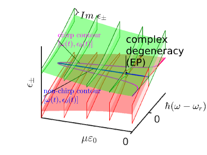
Figure 1: Adiabatic energy surfaces obtained as solutions of a 2x2 Hamiltonian for two coupled states by a CW laser of frequency $\omega$ and laser strength $\varepsilon_{0}$. The energies are complex, since the excited state is a resonance. They consist of the real parts, which are demonstrated by the horizontal surfaces, and the imaginary parts, which are responsible for finite widths $\Gamma_{\pm}=-2{\rm Im}\epsilon_{\pm}$ of the surfaces. The widths are displayed using the vertical “cuts”. We mark a point of complex degeneracy (exceptional point, EP). We also draw possible types of the laser “contours”, which correspond to the definition of the studied Gaussian linearly chirped laser pulses, Eq. 99, 100.

3.2 Quasi-energy split near exceptional point

The quasi-energy split is defined in Eq. 13 which can be also written as,

$$\delta=\Delta\sqrt{1+\lambda^{2}}=\Delta\sqrt{\lambda+i}\cdot\sqrt{\lambda-i},$$ (26)

where

$$\lambda\equiv\frac{\Omega}{\Delta}.$$ (27)

It features two distinct EPs given by

$$\lambda_{EP}=\pm i.$$ (28)

It is known the neigborhood of the EP can be expressed using the Puiseux expansion [37],

$$\delta(\lambda)=\sum\limits_{k=1}^{\infty}a_{k}(\lambda-\lambda_{EP})^{k/2}.$$ (29)

Since we have two EPs, we define two neighborhood expansions such that

$$\delta_{\pm}(\omega,\varepsilon_{0})=\sqrt{\Delta}\,\sqrt{\lambda\pm i}==\sqrt{\omega-\omega_{r}+\frac{i\Gamma}{2\hbar}\pm i\frac{\mu}{\hbar}\varepsilon_{0}},$$ (30)

such that apparently

$$\delta(\omega,\varepsilon_{0})=\delta_{+}\cdot\delta_{-}.$$ (31)

We assume that the quasi-energy split is a product function of the Poiseux series which are associated with $\delta_{+}$ and $\delta_{-}$, respectively, i.e. with the individual EPs.

Persuing this goal we replace $\omega_{r}$ with $\omega_{EP}$ as the reference using Eq. 24,

$$\delta_{\pm}=\sqrt{\omega-\omega_{EP}-\frac{\Gamma}{2\hbar}\frac{{\rm Im}\mu}{{\rm Re}\mu}+\frac{i\Gamma}{2\hbar}\pm i\frac{\mu}{\hbar}\varepsilon_{0}},$$ (32)

and then we combine the terms including $\Gamma$ such that

$$\delta_{\pm}=\sqrt{\omega-\omega_{EP}+i\frac{\Gamma}{2\hbar}\frac{\mu}{{\rm Re}\mu}\pm i\frac{\mu}{\hbar}\varepsilon_{0}}.$$ (33)

Now using the definition of $\varepsilon_{0}^{EP}$ we get (the sign of $\varepsilon_{0}^{EP}$ must correlate with the definition of $\lambda_{EP}$)

$$\delta_{\pm}=\sqrt{(\omega-\omega_{EP})\pm i\frac{\mu}{\hbar}(\varepsilon_{0}-\varepsilon_{0\pm}^{EP})}.$$ (34)

3.3 State exchange along contours encircling EP

It has been shown before that when EP is stroboscopically encircled, the Floquet states are exchanged [37, 16]. Let us show here another short proof to this. We define a general encircling contour such that

$$\omega(\varphi)=\omega_{EP}+\rho(\varphi)\,\cos\left(\varphi\right),$$ (35)

$$\varepsilon_{0}(\varphi)=\varepsilon_{0}^{EP}+\rho(\varphi)\frac{{\rm Re}\mu}{\hbar}\,\sin\left(\varphi\right),$$ (36)

$$\quad 0<\varphi<2\pi,$$ (37)

$$\quad\rho(\varphi)>0,\quad\rho(\varphi)=\rho(\varphi+k\cdot 2\pi).$$ (38)

where $\phi$ represents the angular variable of the encircling. $\rho$ represents the varying distance from the encircled EP, always a positive real defined number. The quasi-energy split along this encircling contour is given by,

$$\delta_{\pm}(\varphi)=\sqrt{\rho(\varphi)}\ \sqrt{\cos(\varphi)\pm i\frac{\mu}{\hbar}\sin(\varphi)}.$$ (39)

We intentionally simplify this expression such that the phase due to the encircling appears before the square root such that

$$\delta_{\pm}(\varphi)=$$ (40)

$$\sqrt{\rho(\varphi)}\ e^{\pm i\varphi/2}\,\sqrt{1\mp\frac{{\rm Im}\mu}{{\rm Re}\mu}\sin(\varphi)e^{\mp i\varphi}}$$ (41)

Assuming $|{\rm Im}\mu|<|{\rm Re}\mu|$, one can use the Taylor expansion for the square root which is periodic in $\phi$ with the period $2\pi$. The exponential prefactor shows that as $\varphi=2\pi$ we get the sign change. The sign change applies for the encircling of one single EP, either $\lambda_{EP}=+i$ or $\lambda_{EP}=-i$. Note that in the physical sense, it is impossible to encircle the EP $\lambda_{EP}=-i$, which corresponds to a negative field amplitude $(-\varepsilon_{0}^{EP})$, encircling of the physical EP therefore is always associated with the sign change of the quasi-energy split.

The sign change of the quasi-energy split $\delta$ upon the encircling implies an exchange between the Floquet states, see the definition of the state energies, Eq. 12. We will assume that the initially occupied state is bound, and it is coupled with a resonance. The quasi-energy split before the interaction is given by the diagonal Floquet Hamiltonian, which is given by Eq. 2 for $\Omega=0$. Using Eqs. 5 and 6 we get,

$$\delta(t_{i})=\left[\omega(t_{i})-\omega_{r}\right]+i\frac{\Gamma}{\hbar}.$$ (43)

For simplicity, let us first assume a contour defined by a the same initial and final frequencies, $\omega(t_{i})=\omega(t_{f})$, and of course it is assumed that the laser amplitude is again zero in the end of such a process. Then in the end of the process, assuming the sign change proved above,

$$\delta(t_{f})=-\left[\omega(t_{f})-\omega_{r}\right]-i\frac{\Gamma}{\hbar}.$$ (44)

Now, in the most simple case, the pulse chirp is linear as we show in Fig. 19, where the final frequency is not the same as the initial one. Yet, even such a process represents an EP encircling where the contour is closed hypothetically through the zero amplitude axis, $\varepsilon_{0}(t>t_{f})\to+0$. Importantly, the Floquet states, being completely decoupled from each other along the gedanken closing contour where $\Omega\to+0$ (Eq. 2), are given by the same field-free solutions from the actual end of the laser interaction up to the end of the hypothetical closing contour. Eq. 44 remains formally the same, but now $\omega(t_{f})\neq\omega(t_{i})$.

In the case of the laser pulse specifically, not only the Floquet states are exchanged, but the field-free states are exchanged as well [16]. This fact is related to the mixing angle $\Theta(t)$ which is defined in Eqs. 10 and 11 and now it depends on the time parameter $t$ through the varying $\varepsilon_{0}(t)$ and $\omega(t)$ in the pulse. $\Omega(t)/\Delta(t)$ has a zero value both on the start and end of the pulse, as the Rabi frequency $\Omega$ is proportional to the field amplitude $\varepsilon_{0}(t)$ (Eq. 4). This implies that $\Theta(t\to\pm\infty)$ is either equal to 0 or $\pi$. $\Theta$ determines the Floquet states as linear combinations of the field free states (the states $|1\rangle$ and $|2\rangle$, optionally including the additional phase factors, Eq. 3). Bearing in mind that the Floquet states are not the same as the EP is stroboscopically encircled ($\varphi=0$ $\to$ $\varphi=2\pi$, Eq. 3), we assess that $\Theta$ is initially given by 0 and finally by $\pi$. The radical change of $\Theta$ is the reason for the necessity of including the non-adiabatic coupling as we discussed in Section 2.3. Combining the asymptotic values of $\Theta$ and the definition of Floquet states in Eq. 10 also represents a proof that the field-free states are always exchanged along the contours defined by finite laser pulses which encircle the EP.

3.4 Dynamical encircling of exceptional point

The state exchange that appears for stroboscopic encircling led to designing and studying realistic systems where the EP was dynamically encircled. The encircling dynamics occurs when the interaction term which takes place in the time-dependent Schrödinger equation Eq. 19 (the interaction term is defined explicitely in Appendix A) is constructed based on the stroboscopic encircling contour $[\omega(t),\varepsilon_{0}(t)]$ defined above. Time-asymmetric state switch represents a characteristic behavior in the systems where EP is dynamically encircled [20, 21, 11, 9, 5, 22, 23, 13, 14, 24, 25]. This phenomenon means that the quantum dynamics is different for the two possible opposite encircling directions, and in particular, the population switch, which we saw for the stroboscopic encircling, is open in one direction but closed in the other.

Let us explain here shortly the reason why this phenomenon takes place (see also Refs. [20, 21, 11]). The quasi-energy split $\delta(t)$ which is in the exponents of the close coupled equations (Eq. 21) includes a non-zero imaginary component due to complex-defined Floquet energies $\epsilon_{\pm}$ (compare Eqs. 9, 12). It is illustrative to split between these components such that,

$$\dot{a}_{\pm}(t)=\mp a_{\mp}(t)\ N_{\mp{\rm Im}\delta}(t)\ e^{\pm\int\limits_{0}^{t}dt^{\prime}{\rm Re}\delta(t^{\prime})},$$ (45)

$$N_{\mp{\rm Im}\delta}(t)=N(t)\ e^{\mp\int\limits_{0}^{t}dt^{\prime}{\rm Im}\delta(t^{\prime})}.$$ (46)

Although it is not usually done this way, we have intentionally assigned the contribution of the imaginary energy components to the non-adiabatic coupling term to show it functioning as a dumping factor that may dump/promote non-adiabatic jumps between the Floquet states, depending on the sign of the exponent. As the sign is opposite for each one of the amplitudes $a_{+}$ and $a_{-}$, respectively, the time-derivative of one of the amplitudes, either $\dot{a}_{+}$ or $\dot{a}_{-}$ on the left hand side of Eq. 46, is always dumped with respect to the other one. Importantly, the effect of damping/promotion is switched with the sign of the propagation time $t$.

3.5 Time-symmetric encircling

The time-asymmetric state switch has been approved in different cases, including an exprimental verification [5], however, the explanation of the time-asymmetry itself [20, 21] suggests that there is a condition which has to be fulfilled should the time-asymmetric switch take place, which is the time-asymmetry of the quasi-energy split $\delta(t)$. Let us suggest the contrary, namely,

$$\delta(-t^{*})=\left[\delta(t)\right]^{*}.$$ (47)

It is the time-integral over quasi-energy split that figures in the exponents in equations, Eqs. 46 or 21. It is suggested that if Eq. 47 is applicable, a time-symmetrical EP encircling dynamics takes place and no time-asymmetric state switch can be observed although EP apparently is encircled.

In order to put our argument on solid grounds, we prove that Eq. 47 implies proper time-symmetry relations for the integral over the quasi-energy split, which is what indeed figures in the exponents of the close-coupled equations Eq. 46. Let us start the derivation by defining the integral over $\delta(t)$ to $(-t^{*})$. As the limit is taken in analogy to the left hand side of Eq. 47, we denote it as $L$,

$$L=\int\limits_{0}^{-t^{*}}dt^{\prime}\,\delta(t^{\prime}).$$ (48)

By substituting $t^{\prime}=-t^{\prime\prime*}$ for the integration variable we get

$$L=-\int\limits_{0}^{t}dt^{\prime\prime*}\,\delta(-t^{\prime\prime*})$$ (49)

and then by using the symmetry of the quasi-energy split defined in Eq. 47 we get

$$L=-\int\limits_{0}^{s}dt^{\prime\prime*}\,\delta^{*}(t^{\prime\prime})$$ (50)

which yields the final time-symmetry relation for the integral over quasi-energy split given by

$$\int\limits_{0}^{-t^{*}}dt^{\prime}\,\delta(t^{\prime})=-\left(\int\limits_{0}^{t}dt^{\prime}\,\delta(t^{\prime})\right)^{*}.$$ (51)

Now as we divide the real and imaginary components of the quasi-energy split assuming integration on the real axis we get

$$\int\limits_{0}^{t}dt^{\prime}\,{\rm Re}\delta(t^{\prime})=-\int\limits_{0}^{-t}dt^{\prime}\,{\rm Re}\delta(t^{\prime}),$$ (52)

$$\int\limits_{0}^{t}dt^{\prime}\,{\rm Im}\delta(t^{\prime})=\int\limits_{0}^{-t}dt^{\prime}\,{\rm Im}\delta(t^{\prime}).$$ (53)

When the second equation is substituted to the close coupled equations Eq. 46, namely to the term defining the non-adiabatic term $N_{\mp{\rm Im}\delta}(t)$, we prove that the obtained exponential damping of the non-adiabatic coupling element is exactly the same upon the exchanged direction of encircling. As the ultimate reason for the time-asymmetric atomic switch is not present, the dynamics follows other rules that are yet to be studied.

To be clear, Eqs. 53 do not prove that the dynamics will be the same when the direction of the encircling is switched because the non-adiabatic coupling element $N(t)$ does not necessarily posses any time-symmetry based on Eq. 47 alone. In some cases, however, it is possible to achieve a fully symmetrical dynamics where the strict condition

$$\Delta(-t^{*})=-[\Delta(t)]^{*},$$ (54)

$$\Omega(-t^{*})=[\Omega(t)]^{*},$$ (55)

is applicable. Eqs. 55 assure the time-symmetry of the non-adiabatic coupling

$$N(-t^{*})=[N(t)]^{*},$$ (56)

as one can show by using Eqs. 16 and 11. The conditions Eqs. 55 imply also the validity of Eq. 47 as one can show by expressing the square of the energy split (Eqs. 13 and 55)

$$\delta^{2}(-t^{*})=\Delta^{2}(-t^{*})+\Omega^{2}(-t^{*})$$ (57)

$$\quad=\Delta^{*2}(t)+\Omega^{*2}(t)=\left[\delta^{2}(t)\right]^{*}.$$ (58)

As the square is a complex conjugated value, the same relation is applicable for the quasi-energy split itself, Eq. 47.

4 Adiabatic perturbation theory

4.1 Boundary conditions for time-dependent wavefunction

Let us consider the initial and final conditions of the time-dependent wavefunction $\psi({\boldsymbol{r}},t)$ defined in Eq. 18. It is assumed that the initial and final wavefunctions, $\psi({\boldsymbol{r}},t\to\pm\infty)$, are associated with the field-free states $|1\rangle$, $|2\rangle$, or more precisely, with the basis set states given in Eq. 3. Namely we set,

$$\Phi_{-}(t\to-\infty)=e^{-\frac{i}{\hbar}E_{2}t+i\omega(t)t}\ |1\rangle,$$ (59)

$$\Phi_{+}(t\to-\infty)=e^{-\frac{i}{\hbar}E_{2}t}\ |2\rangle,$$ (60)

$$\Phi_{-}(t\to\infty)=e^{-\frac{i}{\hbar}E_{2}t}\ |2\rangle,$$ (61)

$$\Phi_{+}(t\to\infty)=e^{-\frac{i}{\hbar}E_{2}t+i\omega(t)t}\ |1\rangle,\$$ (62)

This setting reflects the fact that the adiabatic Floquet states are switched as the EP is encircled. When the definitions of the Floquet states given in Eqs. 62 are substituted to the definition of $\psi({\boldsymbol{r}},t)$ (Eq. 18), for $t\to-\infty$ first, we get,

$$\psi({\boldsymbol{r}},t\to-\infty)=$$ (63)

$$\quad e^{-\frac{i}{\hbar}\int\limits_{0}^{-\infty}dt^{\prime}\epsilon_{-}(t^{\prime})}a_{-}(t\to-\infty)\ e^{-\frac{i}{\hbar}E_{2}t+i\omega(t)t}\ |1\rangle$$ (64)

$$\quad+e^{-\frac{i}{\hbar}\int\limits_{0}^{-\infty}dt^{\prime}\epsilon_{+}(t^{\prime})}a_{+}(t\to-\infty)\ e^{-\frac{i}{\hbar}E_{2}t}\ |2\rangle.$$ (65)

This expression must be compared with the actual initial condition following from the time-evolution of the initial field-free state,

$$\psi({\boldsymbol{r}},t\to-\infty)=e^{-\frac{i}{\hbar}E_{1}t}\ |1\rangle.$$ (67)

This implies the initial values of the non-adiabatic amplitudes

$$a_{-}(t\to-\infty)=e^{\frac{i}{\hbar}\int\limits_{0}^{-\infty}dt^{\prime}\,\epsilon_{-}(t^{\prime})}\ e^{i[\omega_{r}-\omega(t)]t},$$ (68)

$$a_{+}(t\to-\infty)=0.$$ (69)

Note that we used the definition of the resonance frequency $\omega_{r}$ in Eq. 8. The same is done for the final boundary condition where

$$\psi({\boldsymbol{r}},t\to\infty)=$$ (70)

$$\quad e^{-\frac{i}{\hbar}\int\limits_{0}^{\infty}dt^{\prime}\epsilon_{-}(t^{\prime})}a_{-}(t\to\infty)\ e^{-\frac{i}{\hbar}E_{2}t}\ |2\rangle$$ (71)

$$\quad+e^{-\frac{i}{\hbar}\int\limits_{0}^{\infty}dt^{\prime}\epsilon_{+}(t^{\prime})}a_{+}(t\to\infty)\ e^{-\frac{i}{\hbar}E_{2}t+i\omega(t)t}\ |1\rangle$$ (72)

is obtained using Eqs. 18 and 62. The actual wavefunction after the pulse may be written as a linear combination of the two possibly occupied non-interacting field free states such that

$$\psi({\boldsymbol{r}},t\to\infty)=a_{1}\ e^{-\frac{i}{\hbar}E_{1}t}\ |1\rangle+a_{2}\ e^{-\frac{i}{\hbar}{{\cal E}_{2}}t}\ |2\rangle,$$ (74)

where $a_{1,2}$ represent time-independent complex survival and excitation amplitudes, respectively. Note that ${\cal E}_{2}$ is the complex energy of the excited resonance state $|2\rangle$, Eq. 6. From here we get the relation between the non-adiabatic amplitude $a_{-}(t\to\infty)$ to the survival amplitude given by

$$a_{+}(t\to\infty)=a_{1}\ e^{\frac{i}{\hbar}\int\limits_{0}^{\infty}dt^{\prime}\epsilon_{+}(t^{\prime})}e^{i[\omega_{r}-\omega(t)]t}.$$ (75)

4.2 Adiabatic perturbation theory for non-adiabatic amplitudes

By integrating Eq. 21 we obtain the amplitude of the coupled adiabatic state $\Phi_{+}$ , such that

$$a_{+}(t) =a_{+}(t\to-\infty)$$ (76)

$$-\int\limits_{-\infty}^{t}dt^{\prime}\,a_{-}(t^{\prime})N(t)e^{i\int\limits_{0}^{t^{\prime}}dt^{\prime\prime}\delta(t^{\prime\prime})},$$ (77)

which is simplified using the initial conditions Eq. 69 such that

$$a_{+}(t)=-\int\limits_{-\infty}^{t}dt^{\prime}\,a_{-}(t^{\prime})N(t)e^{i\int\limits_{0}^{t^{\prime}}dt^{\prime\prime}\delta(t^{\prime\prime})},$$ (78)

Similarly, $a_{-}(t)$ is given by

$$a_{-}(t) =a_{-}(t\to-\infty)$$ (79)

$$+\int\limits_{-\infty}^{t}dt^{\prime}\,a_{+}(t^{\prime})N(t^{\prime})e^{-i\int\limits_{0}^{t^{\prime}}dt^{\prime\prime}\delta(t^{\prime\prime})}.$$ (80)

By subsequently substituting Eqs. 78 and 80, we obtain the perturbation series,

$$a_{-}(t)=a_{-}(t\to-\infty)\cdot\sum\limits_{j=0,2,...}^{\infty}v^{(j)}(t),$$ (81)

$$a_{+}(t)=a_{-}(t\to-\infty)\cdot\sum\limits_{j=1,3,...}^{\infty}v^{(j)}(t),$$ (82)

where

$$v^{(j+1)}(t)=(-)^{j+1}$$ (83)

$$\times\int_{-\infty}^{t}dt^{\prime}\,v^{(j)}(t^{\prime})\,N(t^{\prime})\,e^{i(-1)^{j}\int_{0}^{t^{\prime}}dt^{\prime\prime}\delta(t^{\prime\prime})}$$ (84)

and

$$v^{(0)}(t)=1.$$ (85)

The prefactor $a_{-}(t\to-\infty)$ has been defined in Eq. 69.

A convergence of the perturbation series is the key assumption here. The adiabatic perturbation series has been proven generally convergent if the less dissipative state is initially occupied, see Refs. [29]. This condition holds in the present case where the initial state is represented by the bound state $|1\rangle$ while the excited state is a resonance, $|2\rangle$. We provide an additional numerical verification of the convergency applicable to the studied case described below based on Gaussian chirped pulses in Appendix D.

4.3 Survival probability

The survival probability $p_{1}$ is defined as the square of the absolute value of the complex survival amplitude $a_{1}$, Eq. 74,

$$p_{1}=|a_{1}|^{2}.$$ (86)

The survival amplitude $a_{1}$ is related to the final non-adiabatic amplitude $a_{+}(t\to\infty)$ through Eq. 75. Using the adiabatic perturbation theory to obtain $a_{+}(t\to\infty)$, Eqs. 82, we get the expression,

$$a_{1} =a_{-}(t\to-\infty)\lim\limits_{t\to-\infty}e^{-i[\omega_{r}-\omega(t)]t}$$ (87)

$$\times e^{-\frac{i}{\hbar}\int\limits_{0}^{\infty}dt^{\prime}\epsilon_{+}(t^{\prime})}\sum\limits_{j=1,3,...}^{\infty}v^{(j)}(t\to\infty).$$ (88)

Using the initial condition Eq. 69 we obtain

$$a_{1} =f\cdot\sum\limits_{j=1,3,...}^{\infty}v^{(j)}(t\to\infty),$$ (89)

where $f$ represents an important normalization and phase factor given by

$$f=\exp\left[-\frac{i}{\hbar}\int\limits_{0}^{\infty}dt^{\prime}\,\epsilon_{+}(t^{\prime})\right]\cdot\exp\left[\frac{i}{\hbar}\int\limits_{0}^{-\infty}dt^{\prime}\,\epsilon_{-}(t^{\prime})\right].$$ (90)

The survival probability within the adiabatic perturbation theory is defined as

$$p_{1}=|f|^{2}\cdot\left|\sum\limits_{j=1,3,...}^{\infty}v^{(j)}(t\to\infty)\right|^{2}.$$ (91)

The normalization and phase factor $f$ can be further simplified for the case of time-symmetric EP encircling defined above in Eq. 55, taking the following steps. First, the exponents of the two terms are merged into one integral such that

$$f=\exp\left[-\frac{i}{\hbar}\int\limits_{0}^{\infty}dt\,\epsilon_{+}(t)+\epsilon_{-}(-t)\right].$$ (92)

Now, we substitute for $\epsilon_{\pm}$ using Eq. 12:

$$f=\exp\left[-\frac{i}{2}\int\limits_{0}^{\infty}dt\,\{\Delta(t)+\Delta(-t)+\delta(t)-\delta(-t)\}\right].$$ (93)

For the time-symmetric EP encircling defined in Eq. 47 we get

$$f=\exp\left[\int\limits_{0}^{\infty}dt\,\{-i\frac{\Delta(t)+\Delta(-t)}{2}+{\rm Im}\delta(t)\}\right].$$ (94)

The dynamical detuning $\Delta(t)$ has the constant imaginary part given by the resonance width $\Gamma$, Eq. 7, thus

$$f=f_{0}\cdot\lim\limits_{T\to\infty}\exp\left[\frac{\Gamma\,T}{2\hbar}+\int\limits_{0}^{T}dt\,{\rm Im}\delta(t)\right],$$ (95)

where $f_{0}$ represents a mere phase factor given by

$$f_{0} =\exp\left[-i\int\limits_{0}^{\infty}dt\,{\rm Re}\left\{\frac{\Delta(t)+\Delta(-t)}{2}\right\}\right]$$ (96)

$$=\exp\left[-i\int\limits_{0}^{\infty}dt\,\left\{\frac{\omega(t)+\omega(-t)}{2}\right\}\right],$$ (97)

with no effect on the calculated survival probability $p_{1}$, Eq. 91. Note that in the case of the fully time-symmetric dynamics which fulfills the more strict conditions Eq. 55,

$$f_{0}=1.$$ (98)

5 Gaussian laser pulse

5.1 Gaussian encircling contour

Let us consider a Gaussian encircling contour defined in the frequency-amplitude plane such that

$$\varepsilon_{0}(t)=\varepsilon_{0}^{max}e^{-t^{2}/2\tau^{2}}$$ (99)

and

$$\omega(t)=\omega_{r}+\alpha t.$$ (100)

This contour leads to the time-symmetric encircling supposed that the transition dipole moment $\mu$ (which codefines the Rabi frequency Eq. 4) is real defined. By substituting definitions Eqs. 99 and 100 to Eqs. 4 and 7 such that we obtain

$$\Omega(t)=\frac{\mu\varepsilon_{0}^{max}}{\hbar}e^{-t^{2}/2\tau^{2}},$$ (101)

$$\Delta(t)=\alpha\,t+\frac{i\Gamma}{2\hbar}.$$ (102)

Using these particular definition and assuming $\mu\in\Re$ we see that the conditions given by Eqs. 55 are satisfied.

5.2 Relative Gaussian pulse parameters

In this Section we derive effective pulse parameters for two-level atoms in linear Gaussian chirps. To this point, the laser pulse is defined via its length $\tau$, chirp $\alpha$, carrier frequency $\omega_{r}$, and maximum peak strength $\varepsilon_{0}^{max}$, as given by Eqs. 99 and 100. These parameters lead to expressions for the quantum dynamics including atomic parameters such as the transition dipole moment $\mu$ and resonance width $\Gamma$.

It is known however that the quantum dynamics can be reduced to a problem which is independent on particular atomic parameters in some cases. Such is the case of non-dissipative two-level atoms in non-chirped pulses where the result of the dynamics is defined by a single effective parameter of a laser pulse, namely the pulse area,

$$\theta=\int\limits_{-\infty}^{\infty}dt\,\Omega(t),$$ (103)

see the pulse area theorem [31, 32, 33] and $\pi$-pulse method in laser control [34].

Let us start our considerations by replacing the physical time $t$ with the effective relative time $s$ such that

$$s=t/\tau,$$ (104)

using the pulse length $\tau$ defined generally as

$$\tau=\frac{\int\limits_{-\infty}^{\infty}dt\,t\,\Omega(t)}{\theta}.$$ (105)

This definition of $\tau$ coincides with the one given in Eq. 99. We redefine the key quantities for the dynamics as functions of $s$. The quasi-energy split and non-adiabatic amplitudes are defined such that

$$\bar{\delta}(s)\equiv\delta(s\tau),$$ (106)

$$\bar{a}_{\pm}(s)\equiv a_{\pm}(s\tau).$$ (107)

The non-adiabatic coupling will be defined as

$$\bar{N}(s)=\tau N(s\tau),$$ (108)

where the prefactor $\tau$ is added due to the derivative (Eq. 459). The non-adiabatic amplitudes satisfy the close-coupled equations obtained from Eqs. 21 which read

$$\dot{\bar{a}}_{\pm}(s)=\mp{\bar{a}}_{\pm}(s)\ \bar{N}(s)\ e^{\pm i\tau\int\limits_{0}^{s}ds^{\prime}\,\bar{\delta}(s^{\prime})}.$$ (109)

Next follows an ad hoc step where we deliberately introduce the pulse area into the evolution equations Eq. 109 as a substitute for $\tau$. We start by rewritting the dynamical Rabi frequency and detuning using the relative time $s$ such that

$$\bar{\Omega}(s)=\frac{\mu\varepsilon_{0}^{max}}{\hbar}\,e^{-s^{2}/2},$$ (110)

$$\bar{\Delta}(s)=\alpha\tau\cdot s+\frac{i\Gamma}{2\hbar}.$$ (111)

As the pulse shape is not changed with the pulse length $\tau$, the dynamical Rabi frequency $\bar{\Omega}(s)$ is now independent on $\tau$. The time-integral in Eq. 103 is redefined using $s$ instead of the physical time such that

$$\theta=\tau\cdot\int\limits_{-\infty}^{\infty}ds\,\bar{\Omega}(s),$$ (112)

showing that $\theta$ is linearly proportional to the pulse length. In particular, it is given by

$$\theta=\frac{\mu\varepsilon_{0}^{max}}{\hbar}\,\tau\,g,\quad g=\int\limits_{-\infty}^{\infty}ds\,e^{-s^{2}/2}=\sqrt{2\pi},$$ (113)

where $g$ is defined by the particular shape of the pulse, here specified by the Gaussian, see Eq. 111.

$$\dot{\bar{a}}_{\pm}(s)=\mp{\bar{a}}_{\pm}(s)\ \bar{N}(s)\ e^{\pm\frac{i\theta}{\sqrt{2\pi}}\int\limits_{0}^{s}ds^{\prime}\,\tilde{\delta}(s^{\prime})},$$ (114)

where $\tilde{\delta}(s)$ is related to $\bar{\delta}(s)$ through the factor,

$$\tilde{\delta}(s)=\frac{\hbar}{\mu\varepsilon_{0}^{max}}\,\bar{\delta}(s).$$ (115)

By assuming that the pulse area $\theta$ is responsible for the exponential factor rather the the pulse length $\tau$, we obtained the factor needed to get the appropriate reduced quasi-energy split $\tilde{\delta}(s)$. From its explicit form given by

$$\tilde{\delta}(s)=\sqrt{e^{-s^{2}}+\left(\frac{\hbar}{\mu\varepsilon_{0}^{max}}\alpha\tau\cdot s+\frac{i\Gamma}{2\mu\varepsilon_{0}^{max}}\right)^{2}}$$ (116)

it is clear that $\tilde{\delta}(s)$ is independent on any atomic parameters in the case of unchirped pulses ($\alpha=0$) and bound-to-bound transitions ($\Gamma=0$). This is in agreement with what is known and has beed stated above that in such a case final populations of the laser driven quantum dynamics only depend on the pulse area. Of course, $\bar{N}(s)$ must prove independent on other laser or atomic parameters as well, which we will show now. $\bar{N}(s)$ is defined by Eq. 108 and also by the definitions of $N(t)$ (Eq. 16) and $\Theta(t)$ (Eq. 11). When we put them together we get

$$\bar{N}(s)=\frac{1}{2}\frac{d\bar{\lambda}(s)}{ds}\frac{1}{1+\bar{\lambda}^{2}(s)},\quad\bar{\lambda}(s)=\frac{\bar{\Delta}(s)}{\bar{\Omega}(s)},$$ (117)

which shows that the non-adiabatic coupling element is a functional of the ratio between the dynamical detuning and Rabi frequency $\bar{\lambda}(s)$. By substituting from Eqs. 111 to the definition of $\bar{\lambda}(s)$ we get

$$\bar{\lambda}(s)=\left(\frac{\hbar}{\mu\varepsilon_{0}^{max}}\alpha\tau\,s+\frac{i\Gamma}{2\mu\varepsilon_{0}^{max}}\right)\,e^{s^{2}/2}.$$ (118)

We can see that $\bar{\lambda}(s)=0$ for the examined case ($\alpha=0$, $\Gamma=0$) which proves the fact $\bar{N}(s)$ is independent of any atomic and laser parameters in that particular case.

Let us define other reduced laser parameters (as if added to a set with the pulse area) for the more general laser-atom two-level dynamics based on the definitions of $\tilde{\delta}(s)$ and $\bar{\lambda}(s)$ which clearly define the system dynamics. We define the relative laser strength $x$ such that

$$x=\frac{2\mu\varepsilon_{0}^{max}}{\Gamma}\equiv\frac{\varepsilon_{0}^{max}}{\varepsilon_{0}^{EP}},$$ (119)

where we used the position of the EP given above in Eq. 25, and the effective chirp $\bar{\alpha}$,

$$\bar{\alpha}=\frac{2\hbar}{\mu}\cdot\frac{\alpha\tau}{\varepsilon_{0}^{max}}.$$ (120)

The definitions of the basic dynamical quantities from Eqs. 114 now read

$$\tilde{\delta}(s)=\sqrt{e^{-s^{2}}+\left(\frac{\bar{\alpha}}{2}\cdot s+\frac{i}{x}\right)^{2}},$$ (121)

$$\bar{\lambda}(s)=e^{s^{2}/2}\cdot\left(\frac{\bar{\alpha}}{2}\,s+\frac{i}{x}\right),$$ (122)

where $\bar{\lambda}(s)$ relates to $\bar{N}(s)$ through Eq. 117.

It is clear that $x$ represents a measure of non-Hermiticity of the quantum dynamics as it reduces the imaginary components in Eqs. 122. This simple analysis alone shows that the general quantum dynamics of the bound-to-resonance transitions coincides with the bound-to-bound systems in the $x\to\infty$ limit. Hermitian regime of the EP encircling can be achieved (for the presently studied fully time-symmetric cases, Eqs. 55), namely by seting large laser intensity $\varepsilon_{0}^{max}\gg\varepsilon_{0}^{EP}$.

6 Singularities in complex time plane

6.1 Effective equations for survival amplitude

The transformation using the effective time $s$ defined in Eq. 104 (above applied only to the evolution equations Eqs. 21 leading to Eqs. 109 and 114) is now applied to the equations for the survival amplitude $a_{1}$ as based on the adiabatic perturbation approach. Eqs. 84 are rewritten as

$$\bar{v}^{(j)}(s)=$$ (123)

$$(-)^{j}\int\limits_{-\infty}^{s}ds^{\prime}e^{-i\tau(-1)^{j}\int\limits_{0}^{s^{\prime}}ds^{\prime\prime}\,\bar{\delta}(s^{\prime\prime})}\,\bar{v}^{(j-1)}(s^{\prime})\bar{N}(s^{\prime})$$ (124)

where $\bar{v}^{(j)}$ correspond with $v^{(j)}$ through

$$\bar{v}^{(j)}(s)=v^{(j)}(s\tau).$$ (126)

and further using the effective quasi-energy split $\tilde{\delta}(s)$ defined above in Eq. 115

$$\bar{v}^{(j)}(s)=$$ (127)

$$(-)^{j}\int\limits_{-\infty}^{s}ds^{\prime}e^{-i\frac{\theta}{\sqrt{2\pi}}\,(-1)^{j}\int\limits_{0}^{s^{\prime}}ds^{\prime\prime}\,\tilde{\delta}(s^{\prime\prime})}\,\bar{v}^{(j-1)}(s^{\prime})\bar{N}(s^{\prime}),$$ (128)

where we have also used Eq. 113 to include the pulse area $\theta$ instead of pulse length $\tau$. Eqs. LABEL:V03 clearly correspond to Eqs. 114.

The survival amplitude $a_{1}$ given in Eq. 89 is rewritten as

$$a_{1}=f\cdot\sum\limits_{j=1,3,\dots}\bar{v}^{(j)}(s\to\infty),$$ (130)

where $f$ has been defined in Eq. 90 and simplified for the time-symmetric case in Eq. 95.

6.2 Quasi-energy split in the real time axis

Let us show how the exponential in Eq. LABEL:V03 behaves for the odd corrections $\bar{v}^{(j)}(s)$ which sum up to the survival amplitude, Eq. 130. The exponent is given by the integral of the quasi-energy split $\tilde{\delta}(s)$ (defined in Eq. 122). The asymptotic behavior of $\tilde{\delta}(s)$ for $s\to\pm\infty$ is given by

$$\tilde{\delta}(s)=sign(s)\cdot\left(\frac{\bar{\alpha}}{2}\cdot s+\frac{i}{x}\right),$$ (131)

which we illustrate in Fig. 2 for two typical values of the parameters $\bar{\alpha}$ and $x$.

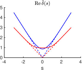
(a) (b)

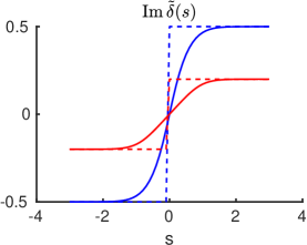
Figure 2: Quasi-energy split for two typical values of the parameters $[x,\bar{\alpha}]$. The red curves correspond to $[5,2]$ (two minima are found on the real part of the split and the limits of the imaginary part are give by $\pm 1/5$)/ The blue curves correspond to $[2,3]$ (single minimum on the real part of the split whereas the imaginary part has the limits given by $\pm 1/3$.

After integrating such a function over the time $s$ we obtain the asymptotic behavior of the real part which is quadratic but it has an inflex point at $s=0$, Fig. 3a, and linear asymptotic behavior of the imaginary part with the minimum at $s=0$, Fig. 3b.

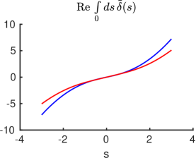
(a) (b)

Figure 3: Integral over quasi-energy split for two typical values of the parameters $[x,\bar{\alpha}]$ corresponding to Fig. 2. Note that the imaginary part has a clear maximum, while the real part has a clear inflexion point.

When we multiply the integral by the imaginary unit to get the exponent, and additionally multiply this by the pulse area $\theta$, see Eq. LABEL:V03, we obtain a bell-type complex function, Fig. 4, where the bell envelope is due to the fact that the imaginary part of the integral goes to infinity in the asymptotic limits where its minimum corresponds to the maximum of the bell function. As $\theta$ is increased, the bell function would become infinitely narrow. This trend is illustrated by increasing $\theta$ from $\theta=4\pi$ to $\theta=50\pi$ when comparing the left and right columns in Fig. 4.

From this point of view, the integrals in Eq. LABEL:V03 for odd corrections $\bar{v}^{(j)}$ seem to reduce to simple integrations over the Dirac $\delta$-function for very large pulse areas $\theta$. However, the complex phase of the exponential function must neither be neglected. The inflexion point shown in Fig. 3a indicates that such a $\delta$-function would occur in the complex plane, $\delta(s-s_{0})$, $s_{0}\in{\cal C}$, where $s_{0}$ would represent a sort of extreme of both the imaginary and real parts of the integral over the quasi-energy split and thus a “zero” of the quasi-energy split.

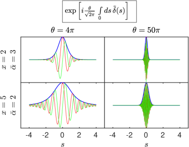
Figure 4: Exponent of the integral Eq. LABEL:V03 for different pulse parameters. This exponent is always a bell-function with maximum at $s=0$. Note that the frequency of oscillations of the complex phase is not constant but it is notably decreased near $s=0$.

6.3 Definition of transition points

Above we suggested that there is likely a “zero” of the quasi-energy split that occurs in the complex time-plane ($s_{0}\in{\cal C}$)

$$\tilde{\delta}(s_{0})=0,$$ (132)

which is reflected as the inflection point and the minimum on the real and imaginary components of the integrated quasi-energy split, respectively (Fig. 3). Such a zero is not a stationary point as one could expect (either a maximum, a minimum, or a saddle point) but rather a branchpoint. While the stationary points are characterized by a finite second derivative of the studied function (i.e. here the first derivative of the quasi-energy split), the first derivative of the quasi-energy split given by

$$\frac{d\tilde{\delta}}{ds}=\left(\frac{\hbar}{\mu\varepsilon_{0}^{max}}\right)^{2}\,\frac{1}{\tilde{\delta}}\,\left(\frac{d\bar{\Delta}}{ds}\bar{\Delta}+\frac{d\bar{\Omega}}{ds}\bar{\Omega}\right)$$ (133)

is rather infinite at the zero of the quasi-energy split $\tilde{\delta}$ which occurs in the denominator.

Importantly, the non-adiabatic element $\bar{N}(s)$ has a pole in the branchpoint $s_{0}$, as follows from Eq. 117 which can be written as

$$\bar{N}(s)=\frac{1}{4i}\frac{d(\bar{\lambda})}{ds}\left(\frac{1}{i+\bar{\lambda}}+\frac{1}{i-\bar{\lambda}}\right),$$ (134)

realizing that

$$\bar{\lambda}(s_{0})=\pm i$$ (135)

at the branchpoints due to the definition

$$\tilde{\delta}(s)=\frac{2\hbar}{x\Gamma}\,\bar{\Delta}(s)\,\sqrt{1+\bar{\lambda}^{2}(s)}.$$ (136)

Namely, the integrand of Eq. LABEL:V03 is singular for $s_{0}$, which makes it impossible to use the previous idea of using Dirac $\delta$-function to simplify the integral over time for large pulse areas $\theta\to\infty$. Rather, a proper application of the residuum theorem represents a possible way to solve this problem, still using the zeros in the complex time plane.

We shall note that the branchpoints in the complex time plane are long known of, being referred to as the transition points (TPs). Although having the same mathematical nature as the exceptional points (EPs), we will distinguish between the EPs as branchpoints defined in the laser parameter plane $[\omega,\varepsilon_{0}]$ , and the TPs in contrast as branchpoints defined in the complex time plane.

6.4 Transition points on the imaginary time axis

Let us search for the TP in the complex time plane in the concrete example given by the linearly chirped Gaussian pulse, where we particularly use Eq. 122 for the quasi-energy split definition. Let us denote the TP by $s_{k}$ as we will soon see that there are more than one TPs in the complex time plane. The TP satisfies the equation,

$$e^{-s_{k}^{2}}+\left(\frac{{\bar{\alpha}}}{2}s_{k}+\frac{i}{x}\right)^{2}=0.$$ (137)

It is reasonable to assume that at least for some parameters $[x,\bar{\alpha}]$ a TP occurs for ${\rm Re}\,s_{k}=0$. Such is the case of $[x=2,\bar{\alpha}=3]$ for which one can see a single minimum on the imaginary part of the quasi-energy split, see the blue curve in Fig. 3b. On the other hand, the second example given by sthe red curve on the same figure indicates two minima, which may possibly correspond to two distinct TPs with different non-zero real parts, ${\rm Re}\,s_{k}\neq 0$.

Let us study for what laser parameters ($x$ and ${\bar{\alpha}}$) Eq. 137 has purely imaginary roots. It is instructive to change the variable $s$ such that

$$s_{k}=i\xi_{k}$$ (138)

and study the real defined roots $\xi_{k}$ instead. Eq. 138 is substituted to Eq. 137:

$$e^{\xi_{k}^{2}}=\left(\frac{{\bar{\alpha}}}{2}\xi_{k}+\frac{1}{x}\right)^{2}.$$ (139)

Apparently, the two sides of Eq. 139 include even, parabolic or parabolic-like ($\exp(z^{2})$), functions, respectively, see Fig. 5. If these parabolas cross each other for real $-is_{0i}\in\Re$, we find the real roots, if they avoid each other, the roots are found in the complex plane.

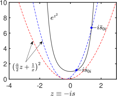
Figure 5: Left and right hand sides of Eq. 139 are compared for the two sets of laser pulse parameters described in Fig. 2. Red color stands for $[x=5,\bar{\alpha}=2]$, while blue color stands for $[x=2,\bar{\alpha}=3]$.

Let us determine the pulse parameters for the situation, where the two parabolas touch each other. At this critical point, the two purely imaginary TPs happen to go to the complex plane. To distinguish the imaginary and complex roots we use different notations for them, $s_{0i}$, $\bar{s}_{0i}$ and $s_{0}$, $\bar{s}_{0}$, respectively. We will obtain the critical laser parameters by requiring that the first derivatives of the left and right hand sides of Eq. 139 are equal:

$$e^{{\left(\xi_{k}^{coal}\right)}^{2}}\xi_{k}=\frac{{\bar{\alpha}}}{2}\left(\frac{{\bar{\alpha}}}{2}\xi_{k}^{coal}+\frac{1}{x}\right).$$ (140)

By combining Eqs. 139 and 140 we obtain

$$\bigg{[}\left(\xi_{k}^{coal}+\frac{2}{{\bar{\alpha}}x}\right)\left(\xi_{k}^{coal}+\frac{1}{{\bar{\alpha}}x}+\sqrt{\frac{1}{({\bar{\alpha}}x)^{2}}+1}\right)$$ (141)

$$\times\quad\left(\xi_{k}^{coal}+\frac{1}{{\bar{\alpha}}x}-\sqrt{\frac{1}{({\bar{\alpha}}x)^{2}}+1}\right)\bigg{]}=0$$ (142)

For ${\bar{\alpha}}>0$, there are two negative and one positive definite roots given by Eq. 142 for any value of $x{\bar{\alpha}}$, while for ${\bar{\alpha}}<0$ it is the other way round. The sign of ${\bar{\alpha}}$ differectiates between clockwise and anti-clockwise encircling of the EP. As the studied dynamics is time-symmetric (see previous Sections), same results must be obtained for the two cases. Therefore we will restrain our study to one case only, in particular assuming ${\bar{\alpha}}>0$.

Let us focus on the positive definite root, $\xi_{k}^{coal}>0$, defined as

$$\xi_{k}^{coal}=\sqrt{\frac{1}{({\bar{\alpha}}x)^{2}}+1}-\frac{1}{{\bar{\alpha}}x},$$ (143)

which occurs when the two TPs $s_{0i}$, $\bar{s}_{0i}$ become a single point, Fig. 5. We will see below that the TPs which are have negative imaginary parts (including the negative roots here) are not relevant to the complex contour integration which will be eventually used to solve the dynamical equations Eq. LABEL:V03, more precisely the first-order perturbation integral.

6.5 Separator in laser parameter plane

By substituting Eq. 143 into Eq. 139, we obtain a separator in the laser parameter space $[{\bar{\alpha}},x]$, which divides between the laser parameters associated with imaginary/complex TPs. The limits on this curve can be calculated analytically; First, if ${\bar{\alpha}}x=0$ then $z=0$ according to Eq. 143, while Eq. 139 specifies that $x=1$ and ${\bar{\alpha}}=0$. Second, if ${\bar{\alpha}}x\to\infty$ then $z=1$ according to Eq. 143, while Eq. 139 specifies that ${\bar{\alpha}}=2\sqrt{e}$ at $x\to\infty$. This is illustrated in Fig. 6.

Figure 6: The laser parameters $[{\bar{\alpha}},x]$ for which the pair of TPs in the complex time plane coalesce on the imaginary axis are represented by the red curve in the main panel. The points $[2,3]$ and $[5,2]$ represent examples of laser parameters, where the TPs lie/lie not on the imaginary axis, respectively. In the limit $x\to\infty$, which is the limit of the rapid adiabatic passage (RAP), the two TPs coalesce for $s_{k}=i$ ($\xi_{k}^{coal}=1$). By substituting this to Eq. 139 and applying again the limit $x\to\infty$ we obtain the asymptotic value of ${\bar{\alpha}}=2e^{1/2}$. This implies a phenomenologically based relation for the occurence of a stable RAP for bound-to-bound transitions (obtained using Eqs. 120 and 113): $\alpha\tau^{2}/\theta>\sqrt{e/2\pi}$. The other limit is represented by ${\bar{\alpha}}=0$, where Eq. 143 implies that the coalescence of TPs occurs on the real axis for $s_{k}=0$ ($\xi_{k}^{coal}=0$). The corresponding laser parameters $[1,0]$ follow from substituting this value to Eq. 139. The three lower panels (a-c) display TPs on the complex time plane for the laser parameters corresponding to the particular points indicated in the main panel. It is demonstrated how the central pair of TPs lay either apart (a) or on (b,c) the imaginary axis; the TPs coalesce in the case (b). Apart from the cental pair of TPs, we also notice the asymptotic series of TPs which seemingly lay on nearly straigh lines.

Let us add here a comment on the physical meaning of the two possible configurations of the TPs that we have just shown taking place in our physical problem. First of all, the two configurations of the TPs reflect what we saw already on the real axis, Fig. 2, where we observed either a single minimum (blue curve) or a double minimum (red curve) on the quasi-energy split. Which one of the situations takes place depends on the laser parameters. The minima of the quasi-energy split indicate nothing else then avoided crossings associated with the increased probability of a non-adiabatic jump.

The problems of non-adiabatic jumps in avoided crossings have been widely studied. The single avoided crossing implies that Landau-Zener formula is applicable in the semiclassical limit [38, 39, 40], while the two subsequent avoided crossings implicate the so called Stückelberg oscillations [41, 42, 43, 30, 44].

Dykhne, Davis, and Pechukas studied a quadratic coupling model for the avoided crossings [27, 28]. They found two different possible configurations of the TPs, which closely corresponds to our findings above. Upon developping the complex plane method, they associated the two different configurations of the TPs with the Landau-Zener and Stückelberg type of non-adiabatic jumps, respectively. In our physical problem, the Landau-Zener regime is manifested as the rapid adiabatic passage (RAP) [45, 46, 47], while the Stückelberg regime corresponds with the regime of Rabi oscillations. This fact will become clearly apparent in the final results of our analysis.

6.6 Asymptotic series of transition points

Let us suppose that the term $i/x$ in Eq. 137 is negligibly small. This case occurs if the process is Hermitian or the contour is far from the EP, i.e. $x\to\infty$, or just if $|s_{k}|$ is large ($|s_{k}|\to\infty$) supposed that ${\bar{\alpha}}$ is non-zero. Then Eq. 137 is approximated by

$$e^{-s_{k}^{2}}=-\left(\frac{{\bar{\alpha}}}{2}\right)^{2}s_{k}^{2},$$ (144)

using

$$\frac{{\bar{\alpha}}}{2}\,|s_{k}|\gg\frac{1}{|x|}.$$ (145)

The left hand side of Eq. 144 is periodic in the complex time plane due to the exponential of imaginary components of $s^{2}$, thus there is a series of TPs $s_{k}$, where the difference between subsequent TPs, $s_{k+1}^{2}$ and $s_{k}^{2}$, is approximately given by $2i\pi$. In a more precise approximation (derived in Appendix E),

$$s_{k}^{2}=k\cdot 2i\pi+i\pi/2-\ln(2k\pi)-2\ln\left(\frac{{\bar{\alpha}}}{2}\right),$$ (146)

$$\quad k\to\infty.$$ (147)

as one can verify by substituting this to Eq. 144. From here we get,

$$s_{k}=\sqrt{k\cdot 2i\pi}\left[1+\frac{i}{4k\pi}\ln\left(\frac{{\bar{\alpha}}^{2}}{2}\,k\pi\right)+\frac{1}{8k}\right],$$ (148)

$$\quad k\to\infty.$$ (149)

The time-symmetry of the problem defined in Eq. 47 implies that the TPs appear in pairs (let us denote them $s_{k}$ and $\bar{s}_{k}$) that are mutually related as

$$\bar{s}_{k}=-s_{k}^{*}, {\rm Re}\,s_{k}>0,\quad{\rm Re}\,\bar{s}_{k}<0.$$ (150)

(The only situation where there is not a pair of TPs occurs for the cases where the TPs lie on the imaginary axis.) The adjoint series to Eqs. 147 and 149 are given by,

$$\bar{s}_{k}^{2}=-k\cdot 2i\pi-i\pi/2-\ln(2k\pi)-2\ln\left(\frac{{\bar{\alpha}}}{2}\right),$$ (151)

$$k\to\infty.$$ (152)

and

$$\bar{s}_{k}=\sqrt{k\cdot 2i\pi}\left[-i+\frac{1}{4k\pi}\ln\left(\frac{{\bar{\alpha}}^{2}}{2}\,k\pi\right)-\frac{i}{8k}\right],$$ (153)

$$\quad k\to\infty.$$ (154)

Although the results given in Eqs. 147–154 have been derived for EPs in the asymptotic limit $k\to\infty$, in practise they represent a good approximation starting from $k=2$ as we demonstrate in Fig. 7.

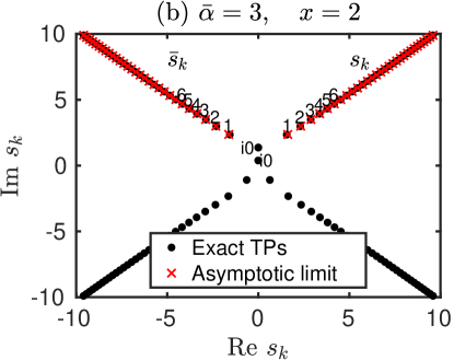
Figure 7: Exceptional points $s_{k}$ and $\bar{s}_{k}$ in the complex plane of dimension-less adiabatic time $s$ are compared with their approximate positions obtained for the asymptotic limit $|s_{k}|\to\infty$ (Eqs. 149 and 154). This approximation is valid for $k>0$, where the symmetrical rule given in Eq. 150 yields the two sets of points, $s_{k}$ and $\bar{s}_{k}$. In contrast, the points $s_{0}$ and $\bar{s}_{0}$ are related by Eq. 150 only for the case of even layout (a), as discussed in Section 6.4, and the asymptotic approximation given Eqs. 149 and 154 is not well defined for $k=0$.

7 Puiseux expansion on the complex time-plane

7.1 Product expansion of the quasi-energy split

We have just proved that there are zeros in the complex time-plane where each one represents a distinct branchpoint. As we have discussed already for the EPs, the potential energy split near any branchpoints is given by the Poiseux expansion. We assume that the quasi-energy split as a function of time, $\tilde{\delta}(s)$, can be also expressed using this expansion such that

$$\tilde{\delta}(s)=\prod\limits_{k}\alpha_{k}(s-s_{k})^{1/2},$$ (155)

where all TPs are included, namely both $s_{k}$ and $\bar{s}_{k}$ as well as the TPs in the lower imaginary half-plain.

7.2 Association of TPs to the EPs for positive and negative laser amplitude

Despite of the fact that the encircling contour in the frequency and laser amplitude plane is directly associated with one of the EPs, namely the one with positive laser amplitude (we refer here to the discussion in Sections 3.1 and 3.2), it is an intriguing mathematical fact that the TPs that occur in the complex time-plane are associated with both of these EPs.

Let us start by assuming that the quasi-energy split $\tilde{\delta}(s)$ includes two different kinds of zeros of either $\tilde{\delta}_{+}(s)$ or $\tilde{\delta}_{-}(s)$, respectively, where the functions $\tilde{\delta}_{\pm}(s)$ are time-dependent equivalents of $\delta_{\pm}(\omega,\varepsilon_{0})$ (Eq. 34, see also Eq. 115 for the relation between $\tilde{\delta}$ and $\bar{\delta}$). Namely, $\tilde{\delta}_{\pm}(s)$ are given by,

$$\tilde{\delta}^{2}_{\pm}(s) =\frac{\mu\varepsilon_{0}^{max}}{\hbar}\left[\bar{\Omega}(s)\pm i\bar{\Delta}(s)\right],$$ (156)

which in the particular studied case reads,

$$\tilde{\delta}^{2}_{\pm}(s)=e^{-s^{2}/2}\pm i\left(\frac{\bar{\alpha}}{2}s+\frac{i}{x}\right).$$ (157)

For the TPs in the positive imaginary half-plane, the even indices of $s_{k}$ and $\bar{s}_{k}$, $k\in\{0,2,\cdots\}$, represent the zeros of $\tilde{\delta}_{+}$, while the odd ones, $k\in\{1,3,\cdots\}$, are associated with $\tilde{\delta}_{-}$. Let us prove this statement for the central TPs, $k=0$, first. Based on the substitution used already above in Eq. 138 we obtain,

$$\tilde{\delta}^{2}_{\pm}(\xi_{k})=e^{\xi_{k}^{2}/2}\mp\left(\frac{\bar{\alpha}}{2}\xi_{k}+\frac{1}{x}\right).$$ (158)

Clearly, the exponential and the term in the bracket are both positive defined, assuming that the central TPs lie on the imaginary axis. The only way how they can add to zero is by substraction, which occurs for $\tilde{\delta}_{+}$. Also in the coalescence, $\tilde{\delta}_{+}=0$ while $\tilde{\delta}_{-}\neq 0$, from which we deduce that even when the central TPs are not purely imaginary, they are still associated with the zeros of $\tilde{\delta}_{+}$, not $\tilde{\delta}_{-}$.

Now, we will explore the higher zeros, $k>0$. According to our previous discussion in Section 6.6, we can neglect the contribution $1/x$. An equivalent of Eq. 144 based on $\tilde{\delta}_{\pm}$ rather then $\tilde{\delta}$ reads,

$$\tilde{\delta}^{2}_{\pm}(s_{k})=e^{-s_{k}^{2}/2}\pm i\frac{\bar{\alpha}}{2}s_{k}.$$ (159)

Now, we substitute for $s_{k}$ using Eqs. 147 and 149 which apply for the limit $k\to\infty$. By using $s_{k}^{2}=2ik\pi+i\pi/2$ in the exponential we see immediately that the exponential is given by $\pm e^{-i\pi/4}$ for even/odd values of $k$. As this is compared with the linear term, one can see that the even values of $k$ are associated with the zeros of $\tilde{\delta}_{+}$, while the odd values of $k$ with $\tilde{\delta}_{-}$. The same could be shown for $\bar{s}_{k}$.

In the negative halfplane, ${\rm Im}\,s_{k}<0$, we could show that odd/even $k$-s (defined in analogy to the positive halfplane) correspond to $\tilde{\delta}_{+}$, $\tilde{\delta}_{-}$, respectively. We will use the knowledge discussed in this Section below when defining non-adiabatic coupling.

7.3 Non-adiabatic coupling as a sum of complex poles

As we have discussed in Section 6, the non-adiabatic coupling element $\bar{N}(s)$ includes poles at the TPs. The Puiseux expansion of the quasi-energy split on the complex time-plane defined in Eq. 155 allows us to relate the non-adiabatic coupling $\bar{N}(s)$ (Eq. 117) to the complex poles more explicitely, namely by rewriting the non-adiabatic coupling as a sum over the poles.

The non-adiabatic coupling element can be written using $\tilde{\delta}^{2}_{\pm}(s)$ such that

$$\bar{N}(s)=\frac{1}{4i}\left(\frac{d\ln\tilde{\delta}^{2}_{+}}{ds}-\frac{d\ln\tilde{\delta}^{2}_{-}}{ds}\right),$$ (160)

which one can prove by substitution from Eq. 156 and then comparing with Eq. 117:

$$\frac{\frac{d\tilde{\delta}^{2}_{+}}{ds}}{\tilde{\delta}^{2}_{+}}-\frac{\frac{d\tilde{\delta}^{2}_{-}}{ds}}{\tilde{\delta}^{2}_{-}}=\frac{\frac{d\bar{\Omega}}{ds}+i\frac{d\bar{\Delta}}{ds}}{\bar{\Omega}+i\bar{\Delta}}-\frac{\frac{d\bar{\Omega}}{ds}-i\frac{d\bar{\Delta}}{ds}}{\bar{\Omega}-i\bar{\Delta}}=$$ (161)

$$\quad 2i\frac{\frac{d\bar{\Delta}}{ds}\bar{\Omega}-\frac{d\bar{\Omega}}{ds}\bar{\Delta}}{\bar{\Omega}^{2}+\bar{\Delta}^{2}}=2i\frac{d\frac{\bar{\Delta}}{\bar{\Omega}}}{ds}\frac{\bar{\Omega}^{2}}{\bar{\Omega}^{2}+\bar{\Delta}^{2}}=$$ (162)

$$\quad 2i\,\frac{d\frac{\bar{\Delta}}{\bar{\Omega}}}{ds}\frac{1}{1+\frac{\bar{\Delta}^{2}}{\bar{\Omega}^{2}}}.$$ (163)

The Puiseux expansions for $\tilde{\delta}_{\pm}(s)$ functions derive from Eq. 155, but now only the TPs with positive/negative imaginary parts are used in the individual expansions,

$$\tilde{\delta}_{\pm}^{2}(s)=\prod\limits_{k}\alpha^{2}_{k\pm}\,(s-s_{k\pm}).$$ (164)

When these expressions for $\tilde{\delta}_{\pm}(s)$ are substituted to the definition of the non-adiabatic coupling in Eq. 160, we obtain the equation

$$\bar{N}(s)=\frac{1}{4i}\sum\limits_{k}\frac{z_{k}}{s-s_{k}},$$ (165)

$$z_{k}=e^{i\,k\pi}\cdot{\rm sign}({\rm Im}\,s_{k}).$$ (166)

Note that this expression is general for two-by-two Hamiltonians and it is not limited to the particular case studied here. The general expression Eq. 166 clearly demonstrates the behavior of $\bar{N}(s)$ near the poles $s_{k}$, which can be derived also using the particular present Hamiltonian as we do in Appendix F.2. It is also obvious that the sum over the first order poles Eq. 166 implies a decaying asymptotic behavior of $\bar{N}(s)$, though it may be hard to prove it analytically (perhaps using the expressions for $s_{k}$ such as Eqs. 149 and 154) that the asymptotics for the present case is actually given by the second order exponential, compare Appendix F.3. We illustrate the function $\bar{N}(s)$ for the present case evaluated numerically in Fig. 8.

Figure 8: These logarithmic plots obtained by numerical evaluation (Appendix F.1, Eq. 459) illustrate non-adiabatic coupling $\bar{N}(s)$ in the complex time-plane. $\bar{N}(s)$, has poles at the TPs which is a general behavior for two-by-two Hamiltonians, Eq. 166. This figure also illustrates that $\bar{N}(s)$ decays in all asymptotes of the complex plane $|s|\to\infty$, compare Appendix F.3. The three different choices of laser parameters ($x$ and ${\bar{\alpha}}$ defined in text) correspond with different layouts of TPs.

7.4 Local Poiseux expansion coefficients

The Poiseux expansion which includes all TPs can be rewritten to describe the close neighborhoods of separate TPs. Such expansions are defined as

$$\tilde{\delta}(s)\bigg{|}_{s\approx s_{k}}=\beta_{k}^{(1)}(s-s_{k})^{1/2}+\beta_{k}^{(2)}(s-s_{k})+\cdots,$$ (167)

First we prove that for most TPs, the even coefficients $\beta_{k}^{(2)}$ have zero values. For this sake we rewrite the above general expansion as,

$$\tilde{\delta}(s)=f_{1}(s)\cdot(s-s_{k})^{1/2}+f_{2}(s).$$ (168)

where $f_{1}(s)$ and $f_{2}(s)$ are polynomial expansions which include either the odd or even expansion coefficients, respectively, being defined by the expressions,

$$f_{1}(s)=\sum\limits_{n=0}^{\infty}\beta_{k}^{(2n+1)}(s-s_{k})^{n},$$ (169)

$$f_{2}(s)=\sum\limits_{n=1}^{\infty}\beta_{k}^{(2n)}(s-s_{k})^{n}.$$ (170)

The square of the quasi-energy split, $\tilde{\delta}^{2}(s)$, using this definition is given by

$$\tilde{\delta}^{2}(s)= f_{1}^{2}(s)\cdot(s-s_{k})$$ (171)

$$+2f_{1}(s)\,f_{2}(s)\cdot(s-s_{k})^{1/2}+f_{2}^{2}(s).$$ (172)

As this is compared to Eq. 155, it is clear that the second term in the equation above must be zero. This may happen for either $f_{1}(s)$ of $f_{2}(s)$ being zero. As long as we assume as first order TP with non-zero first-order expansion coefficient $\beta_{k}^{(1)}$, Eq. 167, $f_{1}(s)$ is non-zero, i.e. $f_{2}(s)=0$. This can be true only if all even expansion coefficient are zero,

$$\beta_{k}^{(2n)}=0.$$ (173)

An exception to this rule occurs when two TPs coalesc; this intriguing special situation will be discussed below.

The coefficients $\beta_{k}^{(2n+1)}$ are related to $\alpha_{k}$ such that

$$\tilde{\delta}^{2}(s) =\alpha_{k}^{2}(s-s_{k})\prod\limits_{l\neq k}\alpha_{l}^{2}(s-s_{l})$$ (174)

$$=(s-s_{k})\cdot\left(\sum\limits_{n=0}\beta_{k}^{(2n+1)}(s-s_{k})^{n}\right)^{2}$$ (175)

$$\frac{d\tilde{\delta}^{2}}{ds} =\alpha_{k}^{2}\prod\limits_{l\neq k}\alpha_{l}^{2}(s-s_{l})$$ (176)

$$+\alpha_{k}^{2}(s-s_{k})\left(\sum\limits_{l\neq k}\frac{1}{s-s_{l}}\right)\prod\limits_{l\neq k}\alpha_{l}^{2}(s-s_{l})$$ (177)

$$\frac{d\tilde{\delta}^{2}}{ds} =\left(\sum\limits_{n=0}\beta_{k}^{(2n+1)}(s-s_{k})^{n}\right)^{2}$$ (179)

$$+2\,(s-s_{k})\cdot\left(\sum\limits_{n=0}\beta_{k}^{(2n+1)}(s-s_{k})^{n}\right)$$ (180)

$$\cdot\left(\sum\limits_{n=0}\beta_{k}^{(2n+3)}(n+1)(s-s_{k})^{n}\right)$$ (181)

Now as we set $s=s_{k}$ we get for the derivative of the square:

$$\frac{d\tilde{\delta}^{2}}{ds}\bigg{|}_{s=s_{k}}=\alpha_{k}^{2}\prod\limits_{l\neq k}\alpha_{l}^{2}(s_{k}-s_{l})=\left(\beta_{k}^{(1)}\right)^{2}$$ (182)

Let us continue in this direction and explore the second derivatives of $\tilde{\delta}^{2}$ at the point $s=s_{k}$.

$$\frac{d^{2}\tilde{\delta}^{2}}{ds^{2}}\bigg{|}_{s=s_{k}} =\alpha_{k}^{2}\left(\sum\limits_{l\neq k}\frac{1}{s-s_{l}}\right)\prod\limits_{l\neq k}\alpha_{l}^{2}(s-s_{l})$$ (183)

$$=4\,\beta_{k}^{(1)}\,\beta_{k}^{(3)}.$$ (184)

And we could continue further to obtain definitions all local Poiseux coefficients $\beta_{k}^{(n)}$ using the positions of TPs $s_{k}$ and their Poiseux coefficients $\alpha_{k}$. Here we obtained the expressions,

$$\beta_{k}^{(1)}=\alpha_{k}\prod\limits_{l\neq k}\alpha_{l}(s_{k}-s_{l})^{1/2},$$ (185)

$$\beta_{k}^{(3)}=\frac{\beta_{k}^{(1)}}{4}\,\sum\limits_{l\neq k}\frac{1}{s_{k}-s_{l}}.$$ (186)

The local expansions effectively describe the quasi-energy split in the vicinity of the particular TP $s_{k}$, but in principle they apply for the whole complex time-plane.

The coefficients for the local expansion, however, become singular when two TPs become very near, see Eq. 186 for $\beta_{k}^{(3)}$, when $s_{l}\to s_{k}$, while the first coefficient $\beta_{k}^{(1)}$ goes to zero. Note that we have shown above that for some specific pulse parameters $\bar{\alpha}$ and $x$, two purely imaginary roots of $\tilde{\delta}(s)$ acquire the same value $s_{0i}=\bar{s}_{0i}=s_{0i}^{coal}$, the TPs actually coalesc. We can assess that near the coalescence of TPs, the local Puiseux expansion is slow converging and possibly efficient and applicable only at infinitesimal distances from the nearly coalescing TPs.

7.5 Coalescence of transition points

Let us discuss the Poiseux expansions at the situation when two TPs, namely $s_{0i}$ and $\bar{s}_{0i}$, actually coalesc. This brings about a change in the order of the Poiseux expansion of $\tilde{\delta}(s)$, Eq. 155 which takes the new form

$$\tilde{\delta}(s)_{coal}=\alpha_{0i}^{(2)}(s-s_{0i}^{coal})\cdot\prod\limits_{k\neq{0}}\alpha_{k}(s-s_{k})^{1/2},$$ (187)

where $\alpha_{0i}^{(2)}$ is the higher-order Puiseux expansion coefficient, while apart from the coalescence the same expansion takes the form,

$$\tilde{\delta}(s)=\alpha_{0}(s-s_{0})^{1/2}\bar{\alpha}_{0}(s-\bar{s}_{0})^{1/2}\cdot\prod\limits_{k\neq{0}}\alpha_{k}(s-s_{k})^{1/2},$$ (188)

where the subscript $(k=0)$ stands also for $(k=0i)$, where the difference of the two cases has been defined above.

In local Puiseux expansion, Eq. 167, the first expansion coefficient $\beta_{0}^{(1)}$ is equal to zero while the second-order coefficient $\beta_{0}^{(2)}$ in non-zero. Using the same argument as for the ususal TPs based on the compact version of the Puiseux expansion where the odd and even coefficients participate in two distinct polynomials $f_{1}(s)$ and $f_{2}(s)$, respectively, see Eqs. 168-170, we assess that $f_{1}(s)=0$, implying that at the coalescence, all odd coefficients in the local Puiseux expansion are equal to zero,

$$\beta_{0}^{(2n+1)}=0.$$ (189)

Again, by comparing the derivatives of $\tilde{\delta}^{2}(s)_{coal}$ based on the product and local Puiseux expansions, we obtain the relation between the higher-order expansion coefficients $\beta_{k}^{(2n)}$ and the TPs positions $s_{k}$ and the coefficients $\alpha_{k}$. The first derivative of $\tilde{\delta}^{2}(s)_{coal}$ with respect to $s$ is equal to zero for $s=s_{0i}^{coal}$, Eq. 187, which is in harmony with our previous findings concerning the TPs on the imaginary time axis (Section 6.4). The second derivative is given by,

$$\frac{d^{2}\tilde{\delta}^{2}(s)_{coal}}{ds^{2}}\bigg{|}_{s=s_{0i}^{coal}}=2\alpha_{0}^{(2)}\left[\prod\limits_{k\neq 0}\alpha_{k}^{2}(s_{0i}^{coal}-s_{k})\right]$$ (190)

$$=2\left(\beta_{0}^{(2)}\right)^{2}$$ (191)

And the third derivative by

$$\frac{d^{3}\tilde{\delta}^{2}(s)_{coal}}{ds^{3}}\bigg{|}_{s=s_{0i}^{coal}}$$ (192)

$$=6\alpha_{0}^{(2)}\left(\sum\limits_{k\neq 0}\frac{1}{s_{0i}^{coal}-s_{k}}\right)\left[\prod\limits_{k\neq 0}\alpha_{k}^{2}(s_{0i}^{coal}-s_{k})\right]$$ (193)

$$=12\,\beta_{0}^{(2)}\,\beta_{k}^{(4)}.$$ (194)

From here we obtain the relations for the expansion coefficients given by

$$\beta_{0}^{(2)}=\sqrt{\alpha_{0}^{(2)}}\,\prod\limits_{k\neq 0}\alpha_{k}(s_{0i}^{coal}-s_{k})^{1/2},$$ (195)

$$\beta_{0}^{(4)}=\frac{\beta_{k}^{(2)}}{2}\,\sum\limits_{k\neq 0}\frac{1}{s_{0i}^{coal}-s_{k}}.$$ (196)

7.6 Time-symmetry relations for local Puiseux expansion coefficients

In the case of time-symmetric systems defined above by Eq. 47 we can define a relation between the Poiseux expansion coefficients corresponding to the symmetrical pairs of TPs, $s_{k}$ and $\bar{s}_{k}$, Eq. 150.

Let us start with the relation between the first order expansion coefficients $\beta_{k}^{(1)}$ vs. $\bar{\beta}_{k}^{(1)}$. Any point $s$ near $s_{k}$ can be symmetrically projected to a point $\bar{s}$ near $\bar{s}_{k}$ as we show in Fig. 9. The value of the quasienergy split at the point $s$ is given by

$$\tilde{\delta}(s)=\beta_{k}^{(1)}(s-s_{k})^{1/2}+\beta_{k}^{(3)}(s-s_{k})^{3/2}+\cdots,$$ (197)

whereas the value at the point $\bar{s}$ is given by

$$\tilde{\delta}(\bar{s})=\bar{\beta}_{k}^{(1)}(\bar{s}-\bar{s}_{k})^{1/2}+\bar{\beta}_{k}^{(3)}(\bar{s}-\bar{s}_{k})^{3/2}+\cdots.$$ (198)

Based on Eq. 47 we can substitute in the second equation such that

$$[\tilde{\delta}(s)]^{*}=\bar{\beta}_{k}^{(1)}(\bar{s}-\bar{s}_{k})^{1/2}+\bar{\beta}_{k}^{(3)}(\bar{s}-\bar{s}_{k})^{3/2}+\cdots,$$ (199)

which can be rewriten such that

$$\tilde{\delta}(s)=\bar{\beta}_{k}^{(1)*}(-)^{1/2}(s-s_{k})^{1/2}$$ (200)

$$\quad+\bar{\beta}_{k}^{(3)*}(-)^{3/2}(s-s_{k})^{3/2}+\cdots.$$ (201)

By merely comparing this with Eq. 197 we get

$$\beta_{k}^{(1)}=\bar{\beta}_{k}^{(1)*}(-)^{1/2},$$ (202)

$$\beta_{k}^{(3)}=\bar{\beta}_{k}^{(3)*}(-)^{3/2},\cdots,$$ (203)

where the square root $(-)^{1/2}$ has an unknown sign, corresponding both to $\pm i$. Based on the fact that the complex number $(s-s_{k})^{1/2}$ corresponds to $i(\bar{s}-\bar{s}_{k})^{1/2}$, and not $-i(\bar{s}-\bar{s}_{k})^{1/2}$, see Fig. 9, it is defined that the sign of the imaginary unit must be positive, should the square root $(s-s_{k})^{1/2}$ be defined as shown in Fig. 9. So that the final time-symmetric relation for the Puiseux expansion is given by

$$\bar{\beta}_{k}^{(2n+1)}=-i\,\beta_{k}^{(2n+1)*}(-)^{n}.$$ (204)

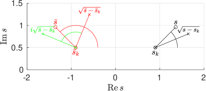
Figure 9: We define the sign of the square root $\sqrt{s-s_{k}}$ using the half of the argument of the complex vector $s-s_{k}$. Importantly, the symmetric counterparts $\bar{s}$ and $\bar{s}_{k}$ are also shown. We demonstrate that the argument $\arg(\bar{s}-\bar{s}_{k})$ is represented by $\arg(s-s_{k})$ substracted from $\pi$. The complex number defined as the square root $\sqrt{\bar{s}-\bar{s}_{k}}$ is shown as a vector originating at $\bar{s}_{k}$ to demonstrate that it actually does not point to any location symmetrically related to the original vector $\sqrt{s-s_{k}}$ started at $s_{k}$. However, when $\sqrt{\bar{s}-\bar{s}_{k}}$ is multiplied by the imaginary unit $(+i)$, then it does represent the symmetric counterpart related to $\sqrt{s-s_{k}}$.

7.7 Complex phase of local Puiseux coefficients

We have proved that the quasi-energy split can be expressed using Puiseux series defined locally based on a single chosen reference TP. The practical way to obtain the local expansion coefficients $\beta_{k}^{(n)}$ is using the analytical expression of the quasi-energy split $\tilde{\delta(s)}$ such as the one given in Eq. 122. By differentiating this definition with respect to $s$ and using Eqs. 182 and 191 we obtain the main coefficients for the first and second order TPs:

$$\beta_{k}^{(1)}=\sqrt{{\bar{\alpha}}\left(\frac{{\bar{\alpha}}}{2}s_{k}+\frac{i}{x}\right)-2s_{k}\,e^{-s_{k}^{2}}},$$ (205)

$$\beta_{0}^{(2)}=\frac{1}{2}\sqrt{{\bar{\alpha}}^{2}-4e^{-(s_{0i}^{coal})^{2}}[1-2(s_{0i}^{coal})^{2}]}.$$ (206)

In the course of further derivations, we will especially need to know what is the complex phase of the first order coefficient, $\beta_{k}^{(1)}$. Such an analysis, which we show in the Appendix G, requires determining the sign of the root in Eq. 206. This sign depends on how we define the roots $(s-s_{k})^{1/2}$, see Fig. 9, and also on the sign of the quasi-energy split on the real time axis.

The complex phases of the local Puiseux coefficients obtained via Eq. 206 and using the sign determined in the Appendix G in some particular limiting cases, are illustrated in Fig. 10. Let us summarize here the limiting cases explicitely:

$$\arg\beta_{0i,low}^{(1)}=-\frac{3\pi}{4}, \arg\beta_{0i,upp}^{(1)}=-\frac{\pi}{4},$$ (207)

$$\arg\beta_{0,coal}^{(1)}=-\frac{\pi}{2}, \arg\bar{\beta}_{0,coal}^{(1)}=0,$$ (208)

$$\arg\beta_{k\to\infty}^{(1)}=-\frac{5\pi}{8}, \arg\bar{\beta}_{k\to\infty}^{(1)}=\frac{\pi}{8}.$$ (209)

The index $(0,coal)$ refers to the central TPs $s_{0}$, $\bar{s}_{0}$ when they are infinitesimally close to the point of their coalescence. Fig. 10a shows how the complex phase is modified for different TPs all the way from this very point ($k=0$) to the limit $k\to\infty$. Fig. 10b illustrates the complex phase of the local Puiseux coefficients where the central TPs reside on the imaginary time axis. Comparing the complex phases of $\beta_{0i,low}^{(1)}$ and $\beta_{0i,upp}^{(1)}$ with the phases of $\beta_{0,coal}^{(1)}$ and $\bar{\beta}_{0,coal}^{(1)}$ shows a sudden change of the complex phases (by $-\pi/4$) of the local Puiseux coefficients upon the coalescence.

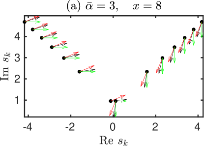
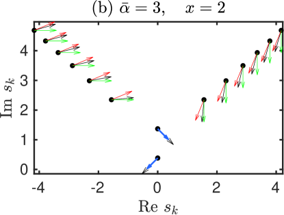
Figure 10: Complex phases of the local Puiseux coefficients $\beta_{k}^{(1)}$ for two different cases of laser pulse parameters ${\bar{\alpha}}$ and $x$ are shown by the black arrows near the corresponding TPs $s_{k}$ and $\bar{s}_{k}$, respectively. The red arrows show the analytical values for the asymptotic limit, $k\to\infty$. The green arrows show the analytical values for the limit where $s_{0}$ and $\bar{s}_{0}$ approach the coalescence. The blue arrows show the analytical values for the case where the TPs lie on the imaginary axis.

8 Residua

In this Section we calculate the residua at the central TPs numerically, while giving an analytical estimate for the residua at the distant TPs. Before doing so we will define a few auxiliary quantities which are useful in such a study and which will be also used throughout the rest of this paper. Namely, we will separate the real and imaginary components of the quasi-energy split, into effective functions $P(s)$ and $Q(s)$, respectively,

$$P(s)=\frac{2\hbar}{\Gamma}{\rm Re}\,\bar{\delta}(s)\equiv x\,{\rm Re}\tilde{\delta}(s),$$ (211)

$$Q(s)=\frac{2\hbar}{\Gamma}{\rm Im}\,\bar{\delta}(s)\equiv x\,{\rm Im}\tilde{\delta}(s).$$ (212)

where we used both definitions of the quasi-energy split in Eq. 107 and of the reduced quasi-energy split in Eqs. 115 and 122. Based on the state exchange in the stroboscopic encircling (see Section 3.3, Eqs. 43 and 44), we get the boundary conditions for $Q(s)$ in the simple form

$$Q(s\to\mp\infty)=\pm 1.$$ (213)

We also define the integral over the quasi-energy split such that

$$\phi(s)=\frac{2\hbar}{\Gamma}{\rm Re}\left[\int\limits_{0}^{s}ds^{\prime}\,\bar{\delta}(s^{\prime})\right]\equiv x\,{\rm Re}\left[\int\limits_{0}^{s}ds^{\prime}\,\tilde{\delta}(s^{\prime})\right],$$ (214)

$$\gamma(s)=\frac{2\hbar}{\Gamma}{\rm Im}\left[\int\limits_{0}^{s}ds^{\prime}\,\bar{\delta}(s^{\prime})\right]\equiv x\,{\rm Im}\left[\int\limits_{0}^{s}ds^{\prime}\,\tilde{\delta}(s^{\prime})\right],$$ (215)

The time-symmetry relation Eq. 53 is rewritten using the functions $\gamma(s)$ and $\phi(s)$ such that

$$\gamma(s)=\gamma(-s^{*}), \phi(s)=-\phi(-s^{*}).$$ (216)

8.1 Residua of the central transition points

Position of central transition points. We solve Eq. 139 for given parameters $[{\bar{\alpha}},x]$ numerically. First, we calculate an initial guess for $\xi_{0}$ (where we note that $s_{0}=i\xi_{0}$, Eq. 138) using the equation

$$\xi_{0}\approx\pm\frac{1}{2}\left({\bar{\alpha}}\pm\sqrt{{\bar{\alpha}}^{2}+8\left(\frac{1}{x}-1\right)}\right),$$ (217)

which is a solution to

$$x\left(1+\frac{\xi_{0}^{2}}{2}\right)\approx\pm\left(\frac{{\bar{\alpha}}x}{2}\xi_{0}+1\right),$$ (218)

which has been obtained from Eq. 139 by applying the square root on both sides of the equation and then approximating the exponential as a parabole. This approximation is correct given the fact that $\xi_{0}^{2}/2$ is rather small, see Figs. 11 (note that $\xi_{0}\equiv-{\rm Im}s_{0}$). This guess is substituted to a standard minimization procedure to solve Eq. 139 numerically exactly. Yet, in some cases it is better to use a starting guess using some known point for similar laser parameters rather then using this quadratic approximation. Numerically calculated positions of the central TPs are displayed in Fig. 11.

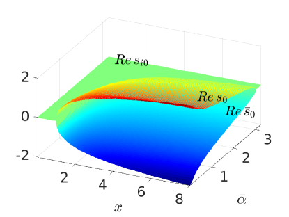
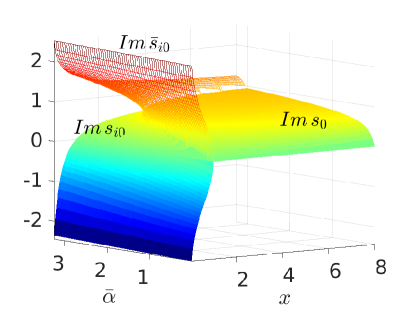
Figure 11: Positions of the central exception points $s_{0}$, $\bar{s}_{0}$ or $s_{i0}$, $\bar{s}_{i0}$ for different laser parameters $x$ and ${\bar{\alpha}}$.

Residua of central transition points. The functions $\gamma(s_{0})$ and $\phi(s_{0})$ for the central TPs $s_{0}$, $\bar{s}_{0}$ or $s_{i0}$, $\bar{s}_{i0}$ are calculated using a numerical integration using the numerically obtained values $s_{0}$, $\bar{s}_{0}$ or $s_{i0}$, $\bar{s}_{i0}$. Fig. 12 confirms numerically the symmetry relations Eqs. 216 for the case of $s_{0}$ and $\bar{s}_{0}$ In the case of $s_{i0}$ and $\bar{s}_{i0}$ these relations are not applicable because the two TPs do not satisfy Eq. 150. However, the numerical calculation indicates that

$$\gamma(s_{i0})=\gamma(\bar{s}_{i0})$$ (219)

holds. This relation will be explained below where we define the equivalue lines as the lines which include points in the complex plane with the same value of $\gamma(s)$. Namely, it will be shown that the TPs $s_{i0}$ and $\bar{s}_{i0}$ are connected by such a line.

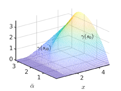
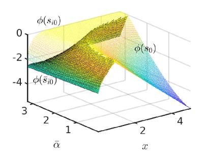
Figure 12: Functions $\gamma(s_{0})$ and $\phi(s_{0})$ at the central exception points $s_{0}$, $\bar{s}_{0}$ or $s_{i0}$, $\bar{s}_{i0}$ for different laser parameters $x$ and ${\bar{\alpha}}$.

8.2 Residua of distant transition points ($k\to\infty$)

In the case of other then the central TPs, $s_{k}$ ($\bar{s}_{k}$) lie far from the center whereas we can assume

$$|s_{k}|\gg 0,\quad\arg s_{k}\approx\frac{\pi}{4}.$$ (220)

Note that the asymptotic value of the argument given in Eq. 220 can be derived immediately using Eq. 147.

We will calculate the residual components $\gamma(s_{k})$ and $\phi(s_{k})$ using the general equations,

$$\gamma(s_{k})=\int\limits_{0}^{s_{k}}\left[({\rm Im}ds)P(s)+({\rm Re}ds)Q(s)\right],$$ (221)

$$\phi(s_{k})=\int\limits_{0}^{s_{k}}\left[({\rm Re}ds)P(s)-({\rm Im}ds)Q(s)\right],$$ (222)

assuming that the complex integration contour avoids any non-analytical point and it does not cross any branchcut. This condition is applicable for the contour which consists of two straight lines – the first part along the real axis, $0\leq s\leq{\rm Re}s_{k}$, and then the second part along the imaginary axis, ${\rm Re}s_{k}\leq s\leq s_{k}$:

$$\gamma(s_{k})=\int\limits_{0}^{{\rm Re}s_{k}}dsQ(s)+\int\limits_{{\rm Re}s_{k}}^{s_{k}}({\rm Im}ds)P(s),$$ (223)

$$\phi(s_{k})=\int\limits_{0}^{{\rm Re}s_{k}}dsP(s)-\int\limits_{{\rm Re}s_{k}}^{s_{k}}({\rm Im}ds)Q(s).$$ (224)

$Q(s)$ and $P(s)$ are generally nontrivial functions which we would get by substituting from Eq. 122 to Eqs. 212. However, we may define the asymptotic forms $Q_{\infty}(s)$ and $P_{\infty}(s)$ which are applicable far from the center of axis along our present integration contour, namely for $s\gg 0$ and $\arg s\leq\frac{\pi}{4}$ (see Eq. 220). The asymptotic forms are given by,

$$P_{\infty}(s)=\frac{{\bar{\alpha}}x}{2}\cdot|{\rm Re}s|, Q_{\infty}(s)=\frac{{\bar{\alpha}}x}{2}\cdot{\rm Im}s\cdot\frac{{\rm Re}s}{|{\rm Re}s|}.$$ (225)

Let us partition Eq. 224 using the asymptotic forms such that

$$\gamma(s_{k})=\int\limits_{0}^{{\rm Re}s_{k}}ds[Q(s)-Q_{\infty}(s)]$$ (226)

$$+\int\limits_{{\rm Re}s_{k}}^{s_{k}}({\rm Im}ds)[P(s)-P_{\infty}(s)]$$ (227)

$$+\int\limits_{0}^{{\rm Re}s_{k}}dsQ_{\infty}(s)+\int\limits_{{\rm Re}s_{k}}^{s_{k}}({\rm Im}ds)P_{\infty}(s),$$ (228)

and

$$\phi(s_{k})=\int\limits_{0}^{{\rm Re}s_{k}}ds[P(s)-P_{\infty}(s)]$$ (229)

$$-\int\limits_{{\rm Re}s_{k}}^{s_{k}}({\rm Im}ds)[Q(s)-Q_{\infty}(s)]$$ (230)

$$+\int\limits_{0}^{{\rm Re}s_{k}}dsP_{\infty}(s)-\int\limits_{{\rm Re}s_{k}}^{s_{k}}({\rm Im}ds)Q_{\infty}(s).$$ (231)

After evaluation of the contribution of the asymptotic behavior we obtain,

$$\gamma(s_{k})=\frac{{\bar{\alpha}}x}{4}\cdot\frac{|{\rm Re}s_{k}|}{{\rm Re}s_{k}}\cdot{\rm Im}(s_{k})^{2}$$ (232)

$$+\int\limits_{0}^{{\rm Re}s_{k}}ds[Q(s)-Q_{\infty}(s)]$$ (233)

$$+\int\limits_{{\rm Re}s_{k}}^{s_{k}}({\rm Im}ds)[P(s)-P_{\infty}(s)],$$ (234)

and

$$\phi(s_{k})=\frac{{\bar{\alpha}}x}{4}\cdot\frac{|{\rm Re}s_{k}|}{{\rm Re}s_{k}}\cdot{\rm Re}(s_{k})^{2}$$ (235)

$$+\int\limits_{0}^{{\rm Re}s_{k}}ds[P(s)-P_{\infty}(s)]$$ (236)

$$-\int\limits_{{\rm Re}s_{k}}^{s_{k}}({\rm Im}ds)[Q(s)-Q_{\infty}(s)].$$ (237)

Let us discuss the nontrivial part of the integration including $Q(s)-Q_{\infty}(s)$ and $P(s)-P_{\infty}(s)$ as the integrands. As for the integration along the real axis of $s$ we refer the reader to Fig. 2, noting that the functions $Q(s)$ and $P(s)$ are related to real and imaginary components of $\tilde{\delta}(s)$ via Eqs. 212. By substracting the asymptotic forms, $Q(s)-Q_{\infty}(s)$ and $P(s)-P_{\infty}(s)$, we have constructed integrands which are zeros in the asymptotes ${\rm Re}s\to\pm\infty$. Assuming that the upper bound ${\rm Re}s_{k}$ represents the asymptotic limit, ${\rm Re}s_{k}\to\infty$, these integrals can be approximated by the assymptotic expressions which we define as,

$$\gamma_{\infty}(x,{\bar{\alpha}})=\int\limits_{0}^{\infty}ds[Q(s;x,{\bar{\alpha}})-Q_{\infty}(s)],$$ (238)

$$\phi_{\infty}(x,{\bar{\alpha}})=\int\limits_{0}^{\infty}ds[P(s;x,{\bar{\alpha}})-P_{\infty}(s)],$$ (239)

and which are independent on the position of the transition point $s_{k}$. The integrals $\gamma_{\infty}(x,{\bar{\alpha}})$ and $\phi_{\infty}(x,{\bar{\alpha}})$ only depend on the pulse parameters $x$ and ${\bar{\alpha}}$ through the dependence of $Q(s)$ and $P(s)$ on these parameters.

Now we shall explore the integrals in the imaginary axis which ends up at the TP $s_{k}$. Due to the fact that the complex argument of $s$ is limited along the integration contour such that

$$0\leq\arg s<\frac{\pi}{4},$$ (240)

compare Eq. 220, the absolute value of the exponential term which is included in the defintion of $\tilde{\delta}(s)$ (Eq. 122) is always smaller or equal to one. Therefore $\tilde{\delta}(s)$ can be approximated using the first order of the Taylor expansion in the asymptotic limit (Eqs. 220) such that

$$\tilde{\delta}(s)\approx\left(z\frac{{\bar{\alpha}}}{2}\cdot s+\frac{i}{x}\right)+\frac{e^{-s^{2}}}{2}\left(z\frac{{\bar{\alpha}}}{2}\cdot s+\frac{i}{x}\right)^{-1},$$ (241)

where

$$z=\frac{{\rm Re}s}{|{\rm Re}s|}.$$ (242)

The exponential term can be written as

$$e^{-s^{2}}=e^{-|s|^{2}\ \cos(2\arg s)}\ e^{-i|s|^{2}\ \sin(2\arg s)},$$ (243)

which shows clearly that the absolute value of the exponential is negligible as $|s|\to\infty$. Therefore the integrals along the imaginary axis in Eqs. 234 and 237 can be omitted. Finally, we obtain,

$$\gamma(s_{k})=\frac{{\bar{\alpha}}x}{4}\cdot\frac{|{\rm Re}s_{k}|}{{\rm Re}s_{k}}\cdot{\rm Im}(s_{k})^{2}+\gamma_{\infty}(x,{\bar{\alpha}}),$$ (244)

and

$$\phi(s_{k})=\frac{{\bar{\alpha}}x}{4}\cdot\frac{|{\rm Re}s_{k}|}{{\rm Re}s_{k}}\cdot{\rm Re}(s_{k})^{2}+\phi_{\infty}(x,{\bar{\alpha}}).$$ (245)

Now it is possible to substitute to Eqs. 244 and 245 using the result in Eq. 147 such that

$$\gamma(s_{k})=\frac{{\bar{\alpha}}x}{4}\pi\left(2k+\frac{1}{2}\right)+\gamma_{\infty}(x,{\bar{\alpha}}),$$ (246)

$$\phi(s_{k})=-\frac{{\bar{\alpha}}x}{4}\ln\left(k\pi\frac{{\bar{\alpha}}^{2}}{2}\right)+\phi_{\infty}(x,{\bar{\alpha}}),$$ (247)

$$\quad\quad k\to\infty.$$ (248)

using the fact that ${\rm Re}s_{k}>0$.

The TPs in the negative real half-axis are denoted as $\bar{s}_{k}$ as defined in Eq. 150; an asymptotic approximation $k\to\infty$ for the points $\bar{s}_{k}^{2}$ is given in Eq. 152. By substituting from this equation to Eqs. 244 and 245 and using ${\rm Re}\bar{s}_{k}<0$, we obtain

$$\gamma(\bar{s}_{k})=\frac{{\bar{\alpha}}x}{4}\pi\left(2k+\frac{1}{2}\right)+\gamma_{\infty}(x,{\bar{\alpha}}),$$ (249)

$$\phi(\bar{s}_{k})=\frac{{\bar{\alpha}}x}{4}\ln\left(k\pi\frac{{\bar{\alpha}}^{2}}{2}\right)-\phi_{\infty}(x,{\bar{\alpha}}),$$ (250)

$$\quad\quad k\to\infty.$$ (251)

Note that the results satisfy the symmetry relations

$$\gamma(s_{k})=\gamma(\bar{s}_{k}),$$ (252)

$$\phi(s_{k})=-\phi(\bar{s}_{k}), k\to\infty,$$ (253)

which is in harmony with Eq. 216.

9 Equivalue lines of the residua

9.1 Residuum theorem in the presence of branch cuts

The calculation of the integral Eq. 283 using residuum theorem assumes integrating along a complex contour which avoids the poles, namely the TPs. However, as the TPs represent not only the poles, but also the branchpoints of the quasi-energy split, the infinitesimal circles

$$s_{k}+r\cdot e^{i\varphi},\quad r\to 0,\ 0\leq\varphi<2\pi,$$ (254)

drawn by such an integration contour near each one of the TPs, suffer from the discontinuity,

$$\tilde{\delta}(s_{k}+r\cdot e^{i\varphi})\neq\tilde{\delta}(s_{k}+r\cdot e^{i\varphi+2\pi}),$$ (255)

which follows from the Puiseux expansion (Eq. 167). Note that this point has been discussed in the context of encircling contour in Section 3.3 whereas a similar argument applies here for the integration contour.

The dicontinuity of $\tilde{\delta}(s)$ is reflected in the discontinuity of $\gamma(s)$ and $\phi(s)$ (Eq. 215) which appear in the exponent of the integrand (Eq. 283). This problem can be solved by defining the complex contour which includes also integration along the branchcuts, represented by curves starting at each TP. Such an integration contour will be discussed in more detail below, see Fig. 16 for the typical integration contours.

The introduction of the branchcuts into the integration contour implies that the complex plane is cut by a line which starts at the TP and proceeds all the way to an asymptote. We have demonstrated, see Eq. 225, that $Q(s)$ and $P(s)$ functions are linearly dependent on $s$, which may easily lead to a divergent behavior when integrated up to infinity ($|s|\to\infty$). This could lead to a rather clumsy if not impossible application of the suggested complex contour integration.

It is possible, however, to define curves, associated with a particular TP ($s=s_{k}$), with the specific behavior that $\gamma(s)$ is constant along such curves, while all the change of the integrated function $\tilde{\delta}(s)$ is reflected into the variations of $\phi(s)$. Because $\phi(s)$ is responsible only for the phase of the integrated function (Eq. 283), the complex contour integration along such curves avoids the problem of divergency. Such curves are therefore most suitable to define the intended integration path.

These curves have been proposed before for integration including branchpoints and are refered to either as the equivalue lines or the Stoke’s lines, Refs. [27, 28]. In this Section we explore the asymptotic analytical behavior of the equivalue lines for the particular studied case of the symmetric EP encircling based on the Gaussian contour.

9.2 Definition of equivalue lines

The so called equivalue lines are defined as the curves which

(i) start at the positions of TPs in the complex plane of, $s=s_{k}$, and

(ii) satisfy the condition

$$\gamma(s)-\gamma(s_{k})=0$$ (256)

at any point $s$ on the curve. This means that the exponential term of the integrand (Eq. 283) given by

$$\exp{\left[-\frac{\tau\Gamma}{2\hbar}\left[\gamma(s)-i\phi(s_{k})\right]\right]}.$$

has a constant absolute value along the equivalue lines, which is defined by

$$\exp{\left[-\frac{\tau\Gamma}{2\hbar}\gamma(s_{k})\right]}.$$ (257)

The equivalue lines are defined by the condition:

$${\rm Im}\oint\limits_{s_{k}}^{s}ds^{\prime}\tilde{\delta}(s^{\prime})=0.$$ (258)

9.3 Equivalue lines behavior near the TPs

The condition given by Eq. 258 may be satisfied by different curves emanating from the given TP ($s_{k}$) in the complex time plane depending on the Puiseux order of the TP. Dykhne, Davis, and Pechukas show three different equivalue lines launching from the TPs in their studies [27, 28].

Let us define an infinitesimal contour closely encircling the TP and find for how many points on this circle Eq. 258 is satisfied. We substitute for $\tilde{\delta}(s)$ in Eq. 258 by using the first term in the Puiseux series, Eqs. 167:

$${\rm Im}\oint\limits_{s_{k}}^{s}ds^{\prime}\beta_{k}^{(m)}(s-s_{k})^{\frac{m}{2}}=0,$$ (259)

where $m=2$ for the case of coalescent TP and $m=1$ otherwise. We solve this integral and get

$${\rm Im}\left[\frac{2\beta_{k}^{(m)}}{m+2}(s-s_{k})^{\frac{m}{2}+1}\right]=0.$$ (260)

The imaginary component is equal to zero if the argument of the expression satisfies:

$$\arg{\left(\frac{2\beta_{k}^{(m)}}{m+2}\right)}+\left(\frac{m}{2}+1\right)\arg{(s-s_{k})}=n\pi,$$ (261)

$$\quad n\in Z.$$ (262)

$\arg(s-s_{k})$ represents an angle which defines the slope of the equivalue line as it emanates from the TP. The angle is actually defined by the point which lies on the infinitesimal circular contour and satisfies the condition given by Eq. 258. Using the above equation we obtain the analytical expression for this angle, namely

$$\arg{(s-s_{k})}=2\pi\,\frac{n}{m+2}-\frac{2}{m+2}\,\arg{\left(\frac{2\beta_{k}^{(m)}}{m+2}\right)},$$ (263)

$$\quad 1\leq n\leq(m+2).$$ (264)

Obviously, there are $(m+2)$ possible equivalue lines for every TP. Namely, there are three equivalue lines of non-coalescent TPs ($m=1$), and four equivalue lines for the special case of the coalescent TP ($m=2$).

Let us denote the angles of the emanating equivalue lines defined in Eq. 264 as $\varphi_{kn}$,

$$\varphi_{kn}\equiv\arg(s-s_{k}),$$ (265)

where the integer number $n$ represents a unique identification for each equivalue line. The angles $\varphi_{kn}$ of the most common first Puiseux order TPs are defined as

$$\varphi_{kn}=\frac{2\pi}{3}n-\frac{2}{3}\arg\beta_{k}^{(1)}\ ,$$ (266)

where $n=\{0,1,2\}$. Clearly, the angles are equally distributed along the circle divided by $2\pi/3$, while the first angle associated with $n=0$ is simply given by $-2\arg\beta_{k}^{(1)}/3$.

The complex phases of the first order local Puiseux coefficients have been discussed and calculated in Section 7.7, see particularly Fig. 10 and Eq. LABEL:EQargbeta. Using the numerical results given in Fig. 10 and Eq. 266 we calculate the angles $\varphi_{kn}$ as shown in Fig. 13. Note that the number cycle given by $n\in\{0,1,2\}$ fails to reflect the symmetry of the problem. Namely, if we assume the pairs of $s_{k}$ and $\bar{s}_{k}$, the equivalue lines numbered by the same values of $n$ do not correspond to the pairs of angles $\varphi_{kn}$ and $\pi-\varphi_{kn}$, as one would expect based on Fig. 9. Yet the number cycle proves correct – let us define

$$\bar{\varphi}_{kn}=\arg(s-\bar{s}_{k})=\pi-\varphi_{kn}.$$ (267)

Using the new definition of $\varphi_{kn}$ in Eq. 266 we get

$$\bar{\varphi}_{kn}=\pi-\frac{2\pi}{3}n+\frac{2}{3}\arg\beta_{k}^{(1)}.$$ (268)

Let us use the argument of the local Puiseux coefficient associated with $\bar{s}_{k}$ rather then $s_{k}$, Eq. 204; we obtain,

$$\bar{\varphi}_{kn}=\pi-\frac{2\pi}{3}n-\frac{\pi}{3}-\frac{2}{3}\arg\bar{\beta}_{k}^{(1)}.$$ (269)

From here we see that the symmetric equivalue lines must be started at different parts of the cycle. Supposed that we define the beginning of the cycle for the symmetric counterpart using the symbol $\bar{n}$ such that

$$\bar{\varphi}_{kn}=\frac{2\pi}{3}\bar{n}-\frac{2}{3}\arg\bar{\beta}_{k}^{(1)}.$$ (270)

we get

$$\bar{n}=1-n,$$ (271)

which is in agreement with the asymmetry of numbering apparent from Fig. 13.

The equivalue lines far from the TPs, which are also shown in Fig. 13, represent curves satisfying Eq. 258. They are calculated numerically as the initial value problem using a propagation scheme. We define a real propagation parameter $\lambda$, where the points on the equivalue line $s_{BC}$ satisfy:

$$\frac{d\,s_{BC}(\lambda)}{d\lambda}=\pm\exp\left(-i\arg\tilde{\delta}[s_{BC}(\lambda)]\right),$$ (272)

where $d\lambda=|ds_{BC}|$. The initial point $s_{BC}(d\lambda)$ is obtained using Eq. 264:

$$s_{BC}(d\lambda)=s_{k}+$$ (273)

$$\quad d\lambda\cdot\exp\left[i\left(2\pi\,\frac{n}{m+2}-\frac{2}{m+2}\,\arg{\left(\frac{2\beta_{k}^{(m)}}{m+2}\right)}\right)\right].$$ (274)

(a)
(b)

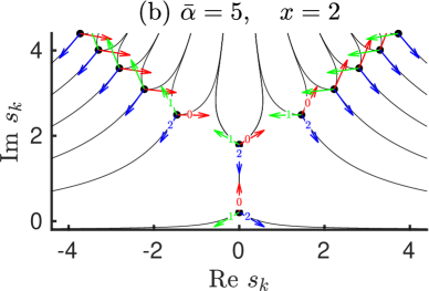
Figure 13: Equivalue lines (black curves) represent lines where the integral over quasienergy split has the same imaginary value as in the corresponding TP. (Such lines will be very important below for the definition of integration contours in the complex time plane as the integrand is non-divergent along these particular lines.) The number of equivalue lines associated with a given TP is defined by the TP Puiseux order. Mostly encountered first order TPs are associated with three equivalue lines. The three equivalue lines are uniquely identified by the index $n$, which is associated with the complex phase of the local Puiseux coefficient and the angle of the emanating equivalue line (denoted by the colored arrows). The values of $n$ are denoted by different colors ($n=0$ – red, $n=1$ – green, $n=2$ – blue).

9.4 Asymptotic behavior of the equivalues lines

As one can see from the numerical calculation shown in Fig. 13, the equivalue lines approach the real axis of $s$ (in the case of the “green” set) or the imaginary axis of $s$ (in the case of the “red” and “blue” sets) in the asymptotes. Below we show the exact analytical asymptotic relations.

Let us start with the equivalue lines approaching the imaginary time axis. In this limit, ${\rm Im}\,s\to\infty$, $\tilde{\delta}(s)$ is approximated by the exponential term,

$$\tilde{\delta}(s)\approx\pm e^{-s^{2}/2},$$ (276)

as follows from Eq. 122. The asymptotic form of $\tilde{\delta}(s)$ enters the definition of the equivalue line on the right hand side of Eq. 272 through its complex phase. By performing appropriate analytical steps which are given in Appendix H.1, we get the asymptotic expression

$${\rm Re}s_{BC}=\frac{(n\pm 1/2)\pi}{{\rm Im}s_{BC}}.$$ (277)

The asymptotic expression given by Eq. 277 is illustrated in Fig. 14.

Now, a very similar procedure is used for the equivalue lines which are parallel to the real axis. Here we use the assumption ${\rm Re}\,s\to\infty$ and $\tilde{\delta}(s)$ is approximated by,

$$\tilde{\delta}(s)\approx\pm\left(\frac{{\bar{\alpha}}}{2}\cdot s+\frac{i}{x}\right).$$ (278)

based on its definition Eq. 122. By doing the appropriate analytical derivation as described in Appendix H.2, we obtain the asymptotic relation given by,

$${{\rm Im}s}=\frac{c_{k}}{{\rm Re}s}-\frac{2}{{\bar{\alpha}}x},\quad{\rm Re}s>0,$$ (279)

where the constant $c_{k}$ remains undetermined. Eq. 279 shows that the equivalue lines approach asymptotically to the line parallel to the real time axis lying at ${\rm Im}\,s=-2/({\bar{\alpha}}x)$ which is in accord with the numerical result (Fig. 13).

The unknown constants $c_{k}$ would determine the points $s_{k0}$ where the equivalue lines cross with the real axis such that

$$s_{0k}=(\pm)\frac{{\bar{\alpha}}\,x\,c_{k}}{2}.$$ (280)

The constants $c_{k}$ can be determined for large indices $k$, where one can assume that the asymptotic form of equivalue lines Eq. 279 is valid including the TP $s_{k}$ itself. Using the knowledge of the positions of $s_{k}$ for the asymptotic regime $k\gg 1$ as given in Eq. 149, we get an analytical relation for the constants $c_{k}$ given by

$$c_{k}\approx(k\pi+\frac{\pi}{4})+(k\pi+\frac{\pi}{4})^{1/2}\left(1-\frac{\ln(k{\bar{\alpha}}\pi)}{4\pi k}\right).$$ (281)

The details of the derivation are given in Appendix H.3. The qualitative and even quantitative precision of such an approximation is illustrated in Fig. 14.

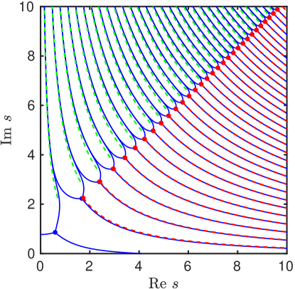
Figure 14: Asymptotic approximations to the equivalue lines given by Eqs. 277 (the minus sign before $1/2$ is used, $n=0,1,...$) and 279 together with Eq. 281 ($k=1,2,...$).

We point out that the crossing points of the equivalue lines with the real axis $s_{0k}$ depend linearly on $k$ in the asymptote, while their distance is determined by the increment ${\bar{\alpha}}\,x/2$, which gets infinite in the Hermitian case where the limit $x\to\infty$ is applicable. Additionally, the equivalue lines asymptotically approach to the real time axis in the Hermitian limit as follows from Eq. 279 as long as $-2/({\bar{\alpha}}\,x)\to 0$.

10 New integration contours for non-Hermitian problem

10.1 Integration contours in Hermitian vs. non-Hermitian cases

This is the key Section of the present paper. We derive here the complex time method for dissipative systems, which include all cases where the EP (which lies in the frequency–field-amplitude plane at the non-zero field-amplitude) is dynamically encircled.

Our present approach is based on the first-order perturbation approximation of the perturbation series discussed above. In this approximation, the sum in Eq. 89 is replaced only by the first term such that

$$v\equiv\sum\limits_{j=1,3,\cdots}\ v^{(j)}(t\to\infty)\approx v^{(1)}(t\to\infty).$$ (282)

To simplify the notation, we denote this expression using the symbol $v$. Thus, the following parts of this study will be based on an analysis of the one-dimensional integral given by

$$v=-\int\limits_{-\infty}^{\infty}dse^{-\frac{\tau\Gamma}{2\hbar}[\gamma(s)-i\phi(s)]}\bar{N}(s).$$ (283)

It has been shown by Davis and Pechukas that the first order approximation leads to an error given by a factor of $3/\pi$, where this result applies in the semiclassical limit, here defined by the large pulse area limit, $\theta\to\infty$ [28]. Their derivation, highly non-trivial as it is, is applicable only for the simpliest case including a single TP. Yet, more then one TP contributions will be included in the analysis of the non-Hermitian case below. Based on these facts, here we limit ourselves to using an ad hoc approach, assuming the first-order approximation having the approximate error of the same factor, which is in agreement with our numerical verifications (Appendix D).

Davis and Pechukas defined a complex contour for Hermitian systems which takes into account only contributions of the TPs that are the closest to the real axis. Such complex contour has been advocated for use also in dissipative systems in Refs. [35, 29, 36]. The discussed complex contours are depicted in Figs. 15) for the odd and even layouts of the TPs. The contours lead along the equivalue lines that start at the central TPs and end asymptotically at ${\rm Re}\,t\to\pm\infty$. In this asymptotic limit, the imaginary part is given by ${\rm Im}\,t\to-2/\bar{\alpha}x$, Eq. 279, which is non-zero for dissipative systems therefore the contour ends up below the real axis. In order to make this contour useful, the interval on the real axis must shrinked to a smaller interval designated by the points of intersections with the equivalue lines defined by $s_{00}$, see Fig. 15. Only supposed that contribution of $|s|>s_{00}$ is negligible, this type of complex contour integration may be justified as an approximation for dissipative systems.

Here we present a different approach to this problem. We define new complex contours based on brachcuts that are placed along other equivalue lines, namely those that end up in the asymptotic limit ${\rm Im}t\to\infty$ as shown in Figs. 16. This leads to a different perception of the quantum dynamics, from a two or single TP-controlled one to the one controlled by the whole complex time plane, because now $all$ TPs contribute to the non-adiabatic amplitudes.

This brings about two implications. First, Hermitian problems represent a special case where the contributions of the TPs inside of the complex plane are mutually canceled due to a destructive interference. Second, only when the pulse area is asymptotically large, the contributions of the two central TPs prevail, and for this matter the use of the Dykhne, Davis, and Pechukas solution is justified in dissipative cases in this limit.

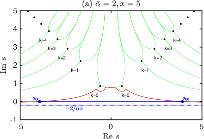
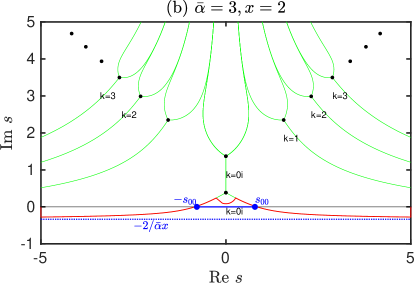
Figure 15: Complex contours originally proposed by Davis and Pechukas as they are applied for the non-Hermitian case. It is shown that only the TP(s) that are nearest to the real axis are touched by the contour, therefore other TPs that lie further from the real axis are irrelevant to the result obtained using this integration. Further it is shown that the complex contour crosses the real axis at the points $s=\pm s_{00}$ as, in the asymptotic limits $s\to\pm\infty$, this contour clings to the line defined by $s=-2/\bar{\alpha}x$ which is colinear with the real axis. This implies that the integration along this contour is not equal to the integral along the real axis. Yet, this integration may represent a good approximation if the integration along the real axis can be reduced to the finite interval designated by $-s_{00}\leq s\leq s_{00}$.

10.2 New integration contours for the two basic layouts of TPs

In Fig. 16 we show a complex contour proposition for two possible different layouts of the central two TPs discussed in Section 6.4. To make a distinction between the two possible layouts we will refer to them as the even layout – where the central TPs $s_{k}$ and $\bar{s}_{k}$ lie apart from the imaginary axis (Fig. 16a), and the odd layout – where the central TPs $s_{0i,low}$ and $s_{0i,upp}$ lie on the imaginary axis (Fig. 16b). Two different integration contours are defined for these layouts.

The proposed contours involve many TPs. The last included TPs $\bar{s}_{k}$ and $s_{k}$, $k\to\infty$, are represented by $k=4$ in Figs. 16 to give a simple illustration. The integrals along such contours consists of the following different types of contributions:

1. integration along circles fully encircling the TPs $s_{k}$ (contributions of residua). These involve all TPs except the last included ones ($k=4$) in the case the even layout, Fig. 16a. In the case of the odd layout, another exception is represented by the TP $s_{0i,upp}$, Fig. 16b. Partial residual contributions are calculated for these exceptions.

2. integration along the two sides of the same branchcuts (branchcut contributions). The branchcut contributions involve both incomming and outgoing integration contours. Such contributions are relevant for all TPs except for the last included TPs ($k=4$). The branchcuts are defined by particular equivalue lines which are identified by both the $k$ index of the TP and the $n$ index of the equivalue line, see Fig. 13. Typically, $n=0$ for the branchcuts in the positive real half-plane and $n=3$ in the negative real half-plane, compare Figs. 15 and 13. In the case of the odd layout, the branchcut for the TPs lying on the imaginary time axis, $s_{0i,low}$ and $s_{0i,upp}$, is defined as the equivalue line connecting between them. This line is characterized by $n=0$ for the lower TP, while $n=2$ for the upper TP.

3. integration along the closing contours connecting the real and imaginary axes. Evaluation of these contributions is very similar to the two sided branchcut integration. The main difference is represented by the different value of $n$ of the lines connecting to the real axis which is given by $n=2$.

4. integration along the equivalue lines $n=1$ and $n=0$ emanating from $s_{0i,upp}$ which are not branchcuts (in the case of the odd layout). Again, the integration is performed in a very similar way to the integration along the two-sided branchcuts.

5. integration along a connecting contour between two branchcuts in the asymptote ${\rm Im}s\to\infty$. Note that the branchcuts end up asymptotically in the imaginary axis, $s\to i\infty$, as we show in Section 9.4, therefore the complex integration contour avoiding these branchcuts passes through the asymptote, see Fig. 16.

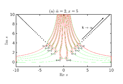
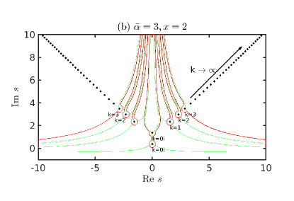
Figure 16: New proposed complex integration contour for dissipative systems for (a) even layout, (b) odd layout. The contours start on the real axis at $-s_{k0}$ and end at $+s_{k0}$, where $k=4$. These contours encompass a finite integration interval on the real axis $-s_{k0}\leq s\leq s_{k0}$, where this interval can be increased by taking the last contributing $k$ to infinity, $k\to\infty$. The region encompassed by the contour excludes all discontinuities on the integrated function, which are represented by the TPs (black circles) and the branchcuts which are intentionally chosen along the equivalue lines (green color).

The contributions of the connecting contours in the asymptotic limit (${\rm Im}s\to\infty$) is new with the new type of integration contours. We prove that the corresponding contributions to the integral is zero in the Appendix I.

11 Analytical expressions for branchcut and residual contributions

11.1 Branchcut contributions

The BC contributions $b_{k}$ are associated with integrals over the lines, which emanate from the TPs:

$$b_{k}^{(j)}=\int\limits_{s_{k}}^{{\rm along\ path}\ k(j)}e^{-\frac{\tau\Gamma}{2\hbar}[\gamma(s)-i\phi(s)]}\,\bar{N}(s)\,ds.$$ (284)

Analytical expressions for these contributions can be obtained for the large pulse area limit.

11.1.1 Large pulse area limit

Let us express the integrated function near the TP ($s=s_{k}$) using the first order expansions for the quasi-energy split $\tilde{\delta}(s)$ as given in Eq. 167 where $\beta_{k}^{(1)}$ is given by Eq. 206; $\bar{N}(s)$ is defined in Eq. 166. In accord with this short range limit, we define a straight line emanating from the TP as

$$s=s_{k}+r\cdot e^{i\varphi_{kn}},$$ (285)

where $\varphi_{kn}$ represents the angle of the integration contour defined by one of the three equivalue lines as given by Eq. 266

$$\varphi_{kn}=\frac{2\pi n}{3}-\frac{2}{3}\arg\beta_{k}^{(1)},$$ (266 revisited)

where $n\in\{0,1,2\}$ determines particularly which one of the three equivalue lines is used.

Let us express the integrated function in the short-range limit using the contour parameter $r$. The non-adiabatic coupling element near the pole is given by Eq. 166. By substituting from Eq. 285 we get,

$$\bar{N}(s)=\frac{z_{k}\,e^{-i\varphi_{kn}}}{4ir}.$$ (286)

The exponent is given by (see definition of $\gamma(s)$ and $\phi(s)$ in Eq. 215)

$$\gamma(s)-i\phi(s)=\gamma(s_{k})-i\phi(s_{k})-ix\int\limits_{s_{k}}^{s}\tilde{\delta}(s)\,ds.$$ (287)

The energy split near the pole is given by the Puiseux series, Eq. 167,

$$\tilde{\delta}(s)=\beta_{k}^{(1)}\cdot(s-s_{k})^{1/2}\,.$$ (167 revisited)

By a substitution from Eq. 285 we get,

$$\tilde{\delta}(s)=\beta_{k}^{(1)}\cdot r^{1/2}e^{i\varphi_{kn}/2},$$ (288)

where $\beta_{k}^{(1)}$ is defined in Eq. 206 From here

$$\gamma(s)-i\phi(s)=$$ (289)

$$\gamma(s_{k})-i\phi(s_{k})-ix\beta_{k}^{(1)}\cdot e^{3i\varphi_{kn}/2}\int\limits_{0}^{r}(r^{\prime})^{1/2}\,dr^{\prime}=$$ (290)

$$\gamma(s_{k})-i\phi(s_{k})-\frac{2ix}{3}\beta_{k}^{(1)}\cdot e^{3i\varphi_{kn}/2}r^{3/2}.$$ (291)

Now if we substitute for $\varphi_{kn}$ from Eq. 266 we get

$$\gamma(s)-i\phi(s)=\gamma(s_{k})-i\phi(s_{k})-e^{in\pi}\frac{2ix}{3}|\beta_{k}^{(1)}|r^{3/2},$$ (292)

which can be further simplified such that

$$\gamma(s)-i\phi(s)=\gamma(s_{k})-i\phi(s_{k})-(-)^{n}\frac{2ix}{3}|\beta_{k}^{(1)}|r^{3/2}.$$ (293)

Note that according to our Eq. 293, where we explored the short range limit, the function $\gamma(s)$ which is defined by the real part of the right hand side, remains constant along the integration contour, $\gamma(s)=\gamma(s_{k})$. This obtained result is correct as it is in accord with the definition of the equivalue lines.

Let us evaluate integral Eq. 284 along the straight line, which is correct very near the TP: First we define

$$b_{k}^{(n)}(s^{\prime})=\int\limits_{s_{k}}^{s^{\prime}({\rm in\ direction\ }\varphi_{kn})}e^{-\frac{\tau\Gamma}{2\hbar}[\gamma(s)-i\phi(s)]}\,\bar{N}(s)\,ds,$$ (294)

and then

$$\lim\limits_{s^{\prime}\to s_{k}}b_{k}^{(n)}(s^{\prime})=$$ (295)

$$\frac{z_{k}}{4i}\,e^{-\frac{\tau\Gamma}{2\hbar}[\gamma(s_{k})-i\phi(s_{k})]}\int\limits_{0}^{|s^{\prime}|}\frac{e^{(-)^{n}\frac{i|\beta_{k}^{(1)}|x\tau\Gamma}{3\hbar}r^{3/2}}}{r}dr,$$ (296)

note that the phase $\exp(-i\varphi_{kn})$ in the definition of $\bar{N}(s)$ (Eq. 286) is canceled due to the change of integration variables ($ds=dr\cdot\exp(i\varphi_{kn})$). This integral is simplified by using the substitution $\rho=r^{3/2}$, which leads to

$$\lim\limits_{s^{\prime}\to s_{k}}b_{k}^{(n)}(s^{\prime})=$$ (298)

$$\frac{z_{k}}{6i}e^{-\frac{\tau\Gamma}{2\hbar}[\gamma(s_{k})-i\phi(s_{k})]}\int\limits_{0}^{|s^{\prime}|^{3/2}}\frac{e^{(-)^{n}\frac{i|\beta_{k}^{(1)}|x\tau\Gamma}{3\hbar}\rho}}{\rho}d\rho.$$ (299)

This is simplified as

$$\lim\limits_{s^{\prime}\to s_{k}}b_{k}^{(n)}(s^{\prime})=\frac{z_{k}}{6i}e^{-\frac{\tau\Gamma}{2\hbar}[\gamma(s_{k})-i\phi(s_{k})]}$$ (300)

$$\times\int\limits_{0}^{|s^{\prime}|^{3/2}}\frac{\cos{\left(\frac{|\beta_{k}^{(1)}|x\tau\Gamma}{3\hbar}\rho\right)}+(-)^{n}\,i\sin{\left(\frac{|\beta_{k}^{(1)}|x\tau\Gamma}{3\hbar}\rho\right)}}{\rho}d\rho$$ (301)

$$=\frac{z_{k}}{6}e^{-\frac{\tau\Gamma}{2\hbar}[\gamma(s_{k})-i\phi(s_{k})]}\bigg{[}-i\,\int\limits_{0}^{|s^{\prime}|^{3/2}}\frac{\cos{\left(\frac{|\beta_{k}^{(1)}|x\tau\Gamma}{3\hbar}\rho\right)}}{\rho}\,d\rho$$ (302)

$$+(-)^{n}\,{\rm Si}{\left(\frac{|\beta_{k}^{(1)}|x\tau\Gamma}{3\hbar}\,|s^{\prime}|^{3/2}\right)}\bigg{]}.$$ (303)

Even though Eq. 303 represents merely a short range integration, it gives us a sufficient information assuming that the factor,

$$\frac{|\beta_{k}^{(1)}|x\tau\Gamma}{3\hbar}\to\infty,$$ (304)

is very large. In such a case, the sine integral function aquires its limiting values at $+\infty$ for $s^{\prime}$ still very close to the TP $s^{\prime}\to s_{k}$. At the same time, the integration over the cosine function is diverging. Eq. 304 which can be also written as

$$\theta\sqrt{\frac{2}{\pi}}\,\frac{|\beta_{k}^{(1)}|}{3}\to\infty,$$ (305)

defines the large pulse area limit, see Appendix J for some concrete equations which apply for the system under the present study.

11.1.2 Integration along two sides of the same branchcut

The branchcut contribution associated with the TP is defined by the incomming and outgoing contours, which happen to be on the different sides of the branchcut. Eq. 303 defines the contribution of the path out of the TP. Then the contribution of the path towards the TP has the opposite sign and also $n$ must be taken as $n\to n+3$, which changes the sign second time but now only for the contribution of the sine function in Eq. 303, while the diverging contributions cancel out. The contribution from the two sides of the branchcut is thus given by

$$b_{kn}=b_{k}^{(n)}-b_{k}^{(n-3)}=$$ (306)

$$\frac{z_{k}\,(-)^{n}}{3}e^{-\frac{\tau\Gamma}{2\hbar}[\gamma(s_{k})-i\phi(s_{k})]}\,{\rm Si}{\left(\frac{|\beta_{k}^{(1)}|x\tau\Gamma}{3\hbar}\,|s^{\prime}|^{3/2}\right)}.$$ (307)

Now, as the divergent part has been taken out, the large pulse area limit defined by Eq. 304 or equivalently Eq. 305 can be readily applied by substituting for the sine integral its limiting value given by $\pi/2$ such that

$$b_{kn}=\frac{z_{k}\,(-)^{n}\,\pi}{6}\,e^{-\frac{\tau\Gamma}{2\hbar}[\gamma(s_{k})-i\phi(s_{k})]}\ .$$ (309)

Eq. 309 represents the branchcut contribution assuming that the branchcut is defined by one of the three equivalue lines. Eq. 309 shows that the branchcut contribution is proportional to the residuum. The sign given by $n$ is altered based on the angle of the equivalue line associated with the branchcut, see Eq. 266.

11.1.3 Closing contours connection the complex contour to the real axis

The complex contour includes equivalue lines starting at each side of the real axis, passing around the last included TP, and continuing along the inner side of the branchcut to a proximity of imaginary axis of time. The contribution of this part of the contour, excluding the semi-circular part near the TP, will be evaluated now.

The contribution of the integration path out of the end TP is given by $b_{k}^{(n)}$, while the integration path to the TP is given by the same equation with the opposite sign. Unlike in the other TPs, now the path winds around the TP not by a full circle but only by $2/3$ of the circle, namely $n\to n-2$, such that the sum of the in and out contributions is defined as

$$b_{k-end}=b_{k}^{(n)}-b_{k}^{(n-2)}.$$ (310)

Using the definition Eq. 303 we find out that the two contributions cancel out, therefore the integration paths associated with the end TPs do not contribute,

$$b_{k-end}=0.$$ (311)

Again, by using Eq. 303 we effectively assumed only the close neighborhood of the TP, which is correct in the large pulse area limit.

11.2 Contributions of residua

A contribution associated with encircling a pole is given by

$$r_{k}=-\oint\limits_{\varphi_{kn}\to\varphi_{kn^{\prime}}}e^{-\frac{\tau\Gamma}{2\hbar}[\gamma(s)-i\phi(s)]}\bar{N}(s)\,ds,$$ (312)

where $n$ and $n^{\prime}$ determine the starting and final integration points, as defined by the equivalue lines. The $(-)$ sign is included as it is assumed that the path of $s$ has the clockwise direction, whereas the true integration path has the anti-clockwise direction. The angles $\varphi_{kn}$ are given by Eq. 266. To evaluate this integral, one can use all equations applying for the short-range limit as introduced in Section 11.1.1.

11.2.1 Integrand along closely encircling contour

Following the logic of Section 11.1, we define a position $s$ near the pole such that,

$$s=s_{k}+r\cdot e^{i(\varphi_{kn}+\varphi)},\quad\quad r>0,$$ (313)

where ${\bar{\alpha}}_{1k}$ is given in Eq. 206. We assume that the partial integration contour in Eq. 312 encircles the pole at the distance of $r=R$, where $R\to 0$. The non-adiabatic coupling element is given by Eq. 286 such that

$$\bar{N}(s)=\frac{z_{k}e^{-i(\varphi_{kn}+\varphi)}}{4iR},$$ (314)

and the exponent in Eq. 312 is given by

$$\gamma(s)-i\phi(s)=\gamma(s_{k})-i\phi(s_{k})$$ (315)

$$-ix\int\limits_{s_{k}}^{s_{k}+R\cdot e^{i\varphi_{kn}}}\bar{\delta}(s)\,ds$$ (316)

$$-ix\oint\limits_{s_{k}+R\cdot e^{i\varphi_{kn}}}^{s_{k}+R\cdot e^{i(\varphi_{kn}+\varphi)}}\bar{\delta}(s)\,ds.$$ (317)

The energy split near the pole is given by the Puiseux series (Eq. 167), where we substituted from Eq. 313 using the distance from the pole $r=R$,

$$\tilde{\delta}(s)=\beta_{k}^{(1)}\,R^{1/2}\,e^{i\varphi_{kn}/2}\,e^{i\varphi/2},$$ (318)

which is substituted to Eq. 317. The first integral is evaluated following the derivation in Eqs. 291-293:

$$\gamma(s)-i\phi(s)=\gamma(s_{k})-i\phi(s_{k})-e^{in\pi}\frac{2ix}{3}|\beta_{k}^{(1)}|\,R^{3/2}$$ (319)

$$\quad-ix\oint\limits_{s_{k}+R\cdot e^{i\varphi_{kn}}}^{s_{k}+R\cdot e^{i(\varphi_{kn}+\varphi)}}\tilde{\delta}(s)\,ds.$$ (320)

The second integral is simplified such that

$$\gamma(s)-i\phi(s)=\gamma(s_{k})-i\phi(s_{k})-e^{in\pi}\frac{2ix}{3}|\beta_{k}^{(1)}|\,R^{3/2}$$ (321)

$$-ix\,R^{1/2}\beta_{k}^{(1)}\int\limits_{0}^{\varphi}e^{i(\varphi^{\prime}+\varphi_{kn})/2}\,d\varphi^{\prime}\,(iR\cdot e^{i(\varphi^{\prime}+\varphi_{kn})}),$$ (322)

where the expression after $d\varphi^{\prime}$ represents the volume element. This simplifies to

$$\gamma(s)-i\phi(s)=\gamma(s_{k})-i\phi(s_{k})-e^{in\pi}\frac{2ix}{3}|\beta_{k}^{(1)}|\,R^{3/2}$$ (323)

$$\quad-i^{2}xR^{3/2}e^{3i\varphi_{kn}/2}\beta_{k}^{(1)}\int\limits_{0}^{\varphi}e^{3i\varphi^{\prime}/2}\,d\varphi^{\prime}.$$ (324)

By using Eq. 266 one gets

$$\gamma(s)-i\phi(s)=\gamma(s_{k})-i\phi(s_{k})-e^{in\pi}\frac{2ix}{3}|\beta_{k}^{(1)}|\,R^{3/2}$$ (325)

$$\quad-e^{in\pi}i^{2}x|\beta_{k}^{(1)}|\,R^{3/2}\int\limits_{0}^{\varphi}e^{3i\varphi^{\prime}/2}\,d\varphi^{\prime}.$$ (326)

By solving the integral one gets,

$$\gamma(s)-i\phi(s)=\gamma(s_{k})-i\phi(s_{k})-e^{in\pi}\frac{2ix}{3}|\beta_{k}^{(1)}|\,R^{3/2}$$ (327)

$$\quad-e^{in\pi}\frac{2ix}{3}|\beta_{k}^{(1)}|\,R^{3/2}(e^{3i\varphi/2}-1),$$ (328)

which simplifies by term cancellation to:

$$\gamma(s)-i\phi(s)=\gamma(s_{k})-i\phi(s_{k})$$ (329)

$$\quad-e^{in\pi}\frac{2ix}{3}|\beta_{k}^{(1)}|\,R^{3/2}e^{3i\varphi/2}.$$ (330)

11.2.2 Integration

Integral Eq. 312 is simplified in the limit $R\to 0$ using Eqs. 314 and 330 such that

$$r_{k}=-\frac{z_{k}}{4iR}e^{-\frac{\tau\Gamma}{2\hbar}[\gamma(s_{k})-i\phi(s_{k})]}\ (iR\cdot e^{i(\varphi+\varphi_{kn})})$$ (331)

$$\times\int\limits_{\varphi_{kn}}^{\varphi_{kn^{\prime}}}e^{e^{in\pi}\frac{ix\tau\Gamma}{3\hbar}|\beta_{k}^{(1)}|R^{3/2}e^{3i\varphi/2}}e^{-i(\varphi+\varphi_{kn})}\,d\varphi\,,$$ (332)

where the expression after $d\varphi$ is the volume element. The first exponential in the integral goes to one as $R\to 0$, therefore it can be removed. By simplifying we get

$$r_{k}=-\frac{z_{k}}{4}e^{-\frac{\tau\Gamma}{2\hbar}[\gamma(s_{k})-i\phi(s_{k})]}\int\limits_{\varphi_{kn}}^{\varphi_{kn^{\prime}}}d\varphi.$$ (333)

If we substitute for the limits using Eq. 266 we get

$$r_{k}=-z_{k}\,\frac{\pi(n^{\prime}-n)}{6}e^{-\frac{\tau\Gamma}{2\hbar}[\gamma(s_{k})-i\phi(s_{k})]}.$$ (334)

The expression is proportional to the integer difference $(n^{\prime}-n)$, which determines how many thirds $\Delta_{n}$ of a circle are used by the complex contour, such that $\Delta_{n}=n^{\prime}-n$ and clearly, $\Delta_{n}\in\{1,2,3\}$.

$$r_{k}=-z_{k}\,\frac{\pi\Delta_{n}}{6}e^{-\frac{\tau\Gamma}{2\hbar}[\gamma(s_{k})-i\phi(s_{k})]}.$$ (335)

12 Overall contributions of the central vs. asymptotic transition points

12.1 Contributions of time-symmetric pairs of TPs

As we solve here the time-symmetric problem, also the complex integration contour is time symmetric with respect to the sign change of the real part of time $s$. The contributions of both residua and branchcuts may be collected according to the pairs of the time-symmetric TPs.

Let us examine the symmetric relation between the branchcut contributions given by $b_{k}^{(n)}$ associated with $s_{k}$

$$b_{kn}=\frac{z_{k}\,(-)^{n}\,\pi}{6}\,e^{-\frac{\tau\Gamma}{2\hbar}[\gamma(s_{k})-i\phi(s_{k})]}\ ,$$ (309 revisited)

and $\bar{b}_{kn}$ associated with $\bar{s}_{k}$, where $\bar{s}_{k}$ has been defined in Eq. 150. $\bar{b}_{kn}$ is obtained by the substitution $s_{k}\to\bar{s}_{k}$ into Eq. 309:

$$\bar{b}_{kn}=\frac{\bar{z}_{k}(-)^{\bar{n}}\pi}{6}e^{-\frac{\tau\Gamma}{2\hbar}[\gamma(\bar{s}_{k})-i\phi(\bar{s}_{k})]}\ .$$ (336)

$\gamma(\bar{s}_{k})$ and $\phi(\bar{s}_{k})$ are directly related to $\gamma(s_{k})$ and $\phi(s_{k})$ based on the symmetric relations given in Eq. 216 such that

$$\gamma(s_{k})=\gamma(\bar{s}_{k}), \phi(s_{k})=-\phi(\bar{s}_{k}).$$ (337)

The sign $\bar{z}_{k}$ is defined in Eq. 166, show that it is same for the two symmetric TPs. This is also confirmed by substituting $\bar{s}_{k}$ into Eq. 464 defining $z_{k}$ in the Appendix F,

$$\bar{z}_{k}=\left(-\frac{1}{x}+\frac{{\bar{\alpha}}}{2}\,i\bar{s}_{k}\right)\,e^{\bar{s}_{k}^{2}/2}=z_{k}^{*}=z_{k}.$$ (338)

As for $n$ and $\bar{n}$, which define the branchcut equivalue lines, they have been defined above (Eq. 271) such that

$$n=0, \bar{n}=1,$$ (339)

however it is also permitted that either $n$ or $\bar{n}$ is augmented by adding one full cycle such that $n\to n+3$ or $\bar{n}\to\bar{n}+3$, which of course would change the sign of one or both contributions $b_{kn}$ and $\bar{b}_{kn}$, respectively. Due to symmetry reasons we assume that $n=0$ for ${\rm Re}\,s_{k}>0$, whereas

$$\bar{n}=1+3=4.$$ (340)

By putting this together we get,

$$b_{kn}=\bar{b}_{kn}^{*}=\frac{z_{k}\,\pi}{6}\,e^{-\frac{\tau\Gamma}{2\hbar}[\gamma(s_{k})-i\phi(s_{k})]}\ ,$$ (341)

$${\rm for}\ {\rm Re}s_{k}>0.$$ (342)

The two contributions sum up to:

$$b_{kn}^{pair}=b_{kn}+\bar{b}_{kn},$$ (343)

such that

$$b_{kn}^{pair}=\frac{z_{k}\,\pi}{3}\,e^{-\frac{\tau\Gamma}{2\hbar}\,\gamma(s_{k})}\,\cos{\left[\frac{\tau\Gamma}{2\hbar}\,\phi(s_{k})\right]}\ ,$$ (344)

$${\rm for}\ {\rm Re}s_{k}>0.$$ (345)

Let us define the symmetrized residual contributions from the pair of poles at $s_{k}$ and $\bar{s}_{k}$ (Eq. 150) such that

$$r_{k}^{pair}=r_{k}+\bar{r}_{k},$$ (346)

where $\bar{r}_{k}$ corresponds to the pole at $\bar{s}_{k}$ and is formally defined as $r_{k}$ (see Eq. 335):

$$\bar{r}_{k}=-\bar{z}_{k}\,\frac{\pi\bar{\Delta}_{n}}{6}e^{-\frac{\tau\Gamma}{2\hbar}[\gamma(\bar{s}_{k})-i\phi(\bar{s}_{k})]}.$$ (347)

Clearly, $\bar{\Delta}_{n}$ is equal to $\Delta_{n}$ due to the symmetry. In the examined pairs the full circle is encompased by the integration contour such that,

$$\Delta_{n}=\bar{\Delta}_{n}=3.$$ (348)

The other relations for the symmetric counterparts such as $\gamma(\bar{s}_{k})$, $\phi(\bar{s}_{k})$, and $\bar{z}_{k}$, are given in Eqs. 337 and 338. By sustitution from these equations we get

$$\bar{r}_{k}=r_{k}^{*}$$ (349)

From here we get:

$$r_{k}^{pair}=2\,{\rm Re}r_{k}.$$ (350)

Using Eq. 335 which represents the formula for the residual contributions $r_{k}$ we obtain the contribution of the symmetric pair of resisua such that

$$r_{k}^{pair}=-z_{k}\,\pi\,e^{-\frac{\tau\Gamma}{2\hbar}\,\gamma(s_{k})}\ \cos\left[\frac{\tau\Gamma}{2\hbar}\,\phi(s_{k})\right].$$ (351)

We may now evaluate the sum of the residual and branchcut contributions for each symmetric pair. Clearly, the presence of the branchcut reduces the residuum contribution by $1/3$. Let us denote the overall contributions of the symmetric pairs of the TPs as $v_{k}^{pair}$. It is defined as

$$v_{k}^{pair}=-\frac{z_{k}\,2\pi}{3}\,e^{-\frac{\tau\Gamma}{2\hbar}\,\gamma(s_{k})}\,\cos{\left[\frac{\tau\Gamma}{2\hbar}\,\phi(s_{k})\right]}\ ,$$ (352)

$${\rm for}\ {\rm Re}s_{k}>0.$$ (353)

12.2 Contributions of the TPs on the imaginary time axis

While for the even layout, the integration includes predominantly the symmetric pair contributions, in the case of the odd layout, the contributions of the TPs on the imaginary time axis are the most important ones. Note that the magnitude of the TPs contributions will be discussed in detail below.

Let us start with the lower TP, $s_{0i,low}$. The branchcut is given by the equivalue line in the upward direction which is characterized by $n=0$, see Fig. 13b. This value of $n$ is substituted into the definition of the branchcut contribution, Eq. 309. Likewise, we may substitute for the known value of $\phi(s_{0i,low})$, which is equal to zero, see Fig. 12b. Finally we substitute for the sign $z_{0i,low}$, which is positive according to Eq. 166. By doing this we obtain the definition of the branchcut contribution of the lower imaginary TP given by,

$$b_{0i,low}=\frac{\pi}{6}\,e^{-\frac{\tau\Gamma}{2\hbar}\,\gamma(s_{0i,low})}\ .$$ (354)

The residual contribution of the lower TP, $s_{0i,low}$, is given by the full circle, therefore $\Delta_{n}$ in the definition Eq. 335 is given by $\Delta_{n}=3$. By doing the same substitutions used above we obtain

$$r_{0i,low}=-\frac{\pi}{2}e^{-\frac{\tau\Gamma}{2\hbar}\,\gamma(s_{0i,low})}.$$ (355)

The overall TP contribution of $s_{0i,low}$ given by the sum of the residuum and branchcut contribution is defined as

$$v_{0i,low}=-\frac{\pi}{3}e^{-\frac{\tau\Gamma}{2\hbar}\,\gamma(s_{0i,low})}.$$ (356)

Now, we will evaluate the contribution of the upper TP $s_{0i,upp}$ to the integration. The branchcut for $s_{0i,upp}$ is given by the equivalue line in the downward direction ($n=2$ according to Fig. 13). Because of how this branchcut is placed, the value of $\phi(s_{0i,upp})$ is not uniquely defined, but it differs for the two sides of the branchcut: Let us denote these values as $\phi(s_{0i,upp-})$ and $\phi(s_{0i,upp+})$ according to the respective real-time half plane. For this reason we also cannot use Eq. 309 to evaluate the two side branchcut contribution unlike in the other cases. Instead, we will evaluate the sum of the contributions of the equvalue lines pertaining to each of the half-planes separately.

Let us start with the left real half plane (${\rm Re}s<0$). First we calculate the sum of the contributions of the equivalue lines defined by $n=1$ (for the incomming contour) and $n=2$ (for the outgoing contour). The outgoing contribution is defined directly by Eq. 303, while the incomming contour contributes with the opposite sign, therefore the sum is given by

$$b_{0i,upp-}=b_{0i,upp-}^{(2)}-b_{0i,upp-}^{(1)}\,.$$ (357)

This result corresponds with Eq. LABEL:EQBC0, which after a simplification (including the application of the large pulse area limit) yields a contribution equivalent to the two side branchcut integral, Eq. 309. Here $z_{0i,upp}=1$ and $n=2$ such that

$$b_{0i,upp-}=\frac{\pi}{6}\,e^{-\frac{\tau\Gamma}{2\hbar}[\gamma(s_{k})-i\phi_{0i,upp-}(s_{k})]}\ .$$ (358)

The upper TP is partially encircled by the integration contour in the left half plane of time, where $\Delta_{n}=1$ in the definition of the partial residual contribution in Eq. 335. The partial residual contribution of the upper pole in the left half plane of time is given by

$$r_{0i,upp-}=-\frac{\pi}{6}\,e^{-\frac{\tau\Gamma}{2\hbar}[\gamma(s_{0i,upp})-i\phi(s_{0i,upp-})]}\ .$$ (359)

By putting together the branchcut contribution, the partial residuum, and the contribution of the incomming contour following the equivalue line $n=1$, we find out that the overall contribution of the upper TP in the left half plane of time is zero,

$$v_{0i,upp-}=0.$$ (360)

The same is applied for the right half plane of time, where the incomming contour is associated with $n=2$ (the right side of the branchcut), while the outgoing contour is associated with $n=0$, Fig. 13. Note that there is no branchcut crossing when the TP is semiencircled between the two equivalue lines. It is thus correct to use $n=3$ instead of $n=0$ for the contribution of the outgoing contour. The sum of the contributions of the incomming and outgoing contours is given by

$$b_{0i,upp+}=b_{0i,upp+}^{(3)}-b_{0i,upp+}^{(2)}\,,$$ (361)

which is simplified to

$$b_{0i,upp+}=\frac{\pi}{6}\,e^{-\frac{\tau\Gamma}{2\hbar}[\gamma(s_{k})-i\phi_{0i,upp+}(s_{k})]}\ .$$ (362)

The residuum contributes partially as

$$r_{0i,upp+}=-\frac{\pi}{6}\,e^{-\frac{\tau\Gamma}{2\hbar}[\gamma(s_{0i,upp})-i\phi(s_{0i,upp+})]}\ .$$ (363)

Again by summing up all contribution to the integration in the right half plane of time we obtain that the upper TP does not contribute to the overall integral,

$$v_{0i,upp+}=0.$$ (364)

12.3 Contribution of the TPs in the asymptotic limit

Let us consider the contribution of the pair of TPs $s_{k}$, $\bar{s}_{k}$ where $k>0$. To some degree of approximation we may consider those TPs as part of the asymptotic limit, where the values for the integrals $\phi(s_{k})$ and $\gamma(s_{k})$ are given in Eqs. 248. The pair contribution $v_{k}^{pair}$ defined in Eq. 353 is evaluated based on the asymptotic limit such that

$$v_{k}^{pair}\approx-\frac{(-)^{k}\,2\pi}{3}\,e^{-\frac{\tau\Gamma\gamma_{\infty}}{2\hbar}}e^{-\frac{\tau\Gamma}{2\hbar}\,\frac{{\bar{\alpha}}x}{2}\pi\left(k+\frac{1}{4}\right)}\,$$ (365)

$$\times\cos{\left\{\frac{\tau\Gamma}{2\hbar}\,\left[\frac{{\bar{\alpha}}x}{4}\ln\left(k\pi\frac{{\bar{\alpha}}^{2}}{2}\right)-\phi_{\infty}\right]\right\}}\ ,$$ (366)

$$\quad\quad k>0,$$ (367)

where we substituted $z_{k}=(-)^{k}$ using the definition in Eq. 166. The overall contribution of the asymptotic TPs is given by the sum

$$v_{\infty}=\sum\limits_{k=1}^{\infty}v_{k}^{pair}\ ,$$ (368)

In the Hermitian limit, where $x\to\infty$, the contributions of the asymptotic TPs are given by zero, which implies that the dynamics is given only by the positions of the central TPs. This is in agreement with the theory of Dykhne, Davis, and Pechukas, who used an integration contour including only cotributions of the central TPs in the Hermitian case, see Fig. 15.

However, as the system is non-Hermitian, the contribution of the asymptotic TPs is non-zero as we can see. Eq. 367 even suggests that the contribution of the asymptotic TPs is related to the value $2/{\bar{\alpha}}x$, which corresponds to the asymptotic behavior of the equivalue lines, see Fig. 16. Eq. 367 suggests that the role of non-Hermitian contributions thought the asymptotic TPs may be dominant for small chirps and small values of $\tau\Gamma$,

$$\tau\Gamma{\bar{\alpha}}x\to 0.$$ (369)

We leave this suggestion an open question.

12.4 Summary of the complex contour integration

The complex amplitude $v$ defined within the first-order perturbation approach in Eq. 283 has been resolved as a sum of contributions of the individual TPs. We have divided the final sum into separate contributions of the central pair of TPs (either $s_{0}$, $\bar{s}_{0}$ or $s_{0i,low}$, $s_{0i,upp}$, depending on the layout) on one side, and the asymptotic TP pairs ($s_{k}$, $\bar{s}_{k}$, $k>0$) on the other side.

The contribution of the central TPs is defined by Eq. 353 (taking $k=0$ where $z_{k}=1$) and Eq. 356 for the two different layouts. The result can be summarized as,

$$v_{0}=-\frac{2\pi}{3}\,e^{-\frac{\tau\Gamma}{2\hbar}\,\gamma(s_{0})}\times\Phi_{0}(s_{0})\,$$ (370)

where $\Phi_{0}(s_{0})$ represents an interference term, which is active in the case of even layout, where it depends on $\phi(s_{0})$ such that

$$\Phi_{0,even}(s_{0})=\cos{\left[\frac{\tau\Gamma}{2\hbar}\,\phi(s_{0})\right]}\ .$$ (371)

Note that $\phi(s_{0})$ is indirectly but clearly related to the distance of the two TPs $s_{0}$ and $\bar{s}_{0}$. The interference is not present in the case of the odd layout, where the interference term is simply given by

$$\Phi_{0,odd}(s_{0i,low})=\frac{1}{2}\ .$$ (372)

In the case of the odd layout, $s_{0}$ is formally replaced by $s_{0i,low}$ in Eq. 370. It has been proven that the upper central TP $s_{0i,upp}$ does not contribute to the integral therefore takes no part in the expressions for the amplitude $v$ of the physical process. This is in harmony with avoiding this TP when using the integration contour proposed by Dykhne, Davis, and Davis in the Hermitian limit.

We have shown that the contribution of the asymptotic TPs is non-zero in the non-Hermitian case, therefore the integration contour by Dykhne, Davis, and Davis is not exact, see Eq. 367. Yet the contributions of the asymptotic TPs may be considered negligible in the large pulse area limit if the product of the chirp and effective intensity ${\bar{\alpha}}x$ is nonzero.

13 Survival amplitude

13.1 Analytical formulas for survival probability

The survival probility $p_{1}$ has been defined in Section 4.3. It is obtained from the complex amplitude $v$ using Eq. 91 which includes a normalization factor $f$ defined in Eq. 95 and in the text below. By using the expression for the pulse area in the case of Gaussian pulses (Eq. 113) and the definition of $\gamma(s)$ (Eq. 215), we obtain a compact expression for $f$ given by,

$$f=\lim\limits_{s\to\infty}\exp\left[\frac{\theta\left[s+\gamma(s)\right]}{x}\frac{1}{\sqrt{2\pi}\hbar}\right].$$ (373)

As we have stated in the beginning of Section 10.1, we approximate $v$ within the first order of the adiabatic perturbation expansion, $v$ is thus defined in Eq. 283.

Additionally, we will assume that (i) the pulse area is large (Eq. 305), and (ii) the non-Hermitian system is mostly controlled by the central pair of the TPs, i.e. Eq. 369 is not true. This allows us to approximate $v$ as $v_{0}$ given by Eqs. 370-372.

13.1.1 Even layout

The survival probability for the even layout is obtained when $v_{0}$ is defined by Eqs. 371 such that

$$p_{1,even}=f^{2}|v_{0,even}|^{2}$$ (374)

$$=\frac{4\pi^{2}}{9}f^{2}\,e^{-\frac{\tau\Gamma}{\hbar}\gamma(s_{0})}\,\cos^{2}\left[\frac{\tau\Gamma}{2\hbar}\phi(s_{0})\right].$$ (375)

Using the definition of the pulse area Eq. 305 allows us to remove the system dependent parameter $\Gamma$:

$$p_{1,even}=\frac{4\pi^{2}}{9}f^{2}\,\exp{\left[-\frac{2}{\hbar\sqrt{2\pi}}\frac{\theta\,\gamma(s_{0})}{x}\right]}$$ (376)

$$\times\quad\cos^{2}\left[\frac{1}{\hbar\sqrt{2\pi}}\frac{\theta\,\phi(s_{0})}{x}\right].$$ (377)

Eq. 377 shows that the behavior of $p_{1}$ is oscillatory due to the cosine term. The important conclusion following from here is that the even layout of TPs in the complex plane of adiabatic time defines an oscillatory subspace in the plane of the reduced laser parameters $x,{\bar{\alpha}}$.

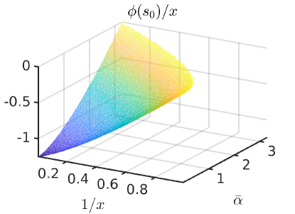
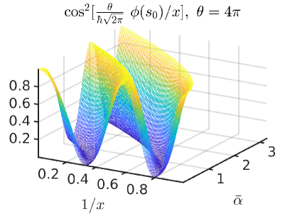
Figure 17: This figure illustrates oscillations of the survival probability, Eq. 377. The argument of the oscillatory function is represented by $\phi(s_{0})/x$. It is found numerically that this function is nearly linear in the plane of $1/x,{\bar{\alpha}}$. The pulse area $\theta=4\pi$.

The exponential modulation of the survival probability $p_{1}$ is given by the values of the exponent in Eq. 377, and additionally, we have to normalize the survival probability by the term $f$, Eq. 373. The overall exponential modulation including both factors is given by

$$\bar{f}=\lim\limits_{s\to\infty}\exp\left[\frac{1}{\hbar\sqrt{2\pi}}\frac{\theta\left[s+\gamma(s)-\gamma(s_{0})\right]}{x}\right].$$ (378)

Based on this we define the integral function $\bar{\gamma}(s_{0})$ such that

$$\bar{\gamma}(s_{0})=\lim\limits_{s\to\infty}[s+\gamma(s)-\gamma(s_{0})],$$ (379)

which controls the exponential decay of the survival probability in the oscillatory regime. Such a function is displayed in Fig. 18.

The final expression for the survival probability in the case of even layout is given by

$$p_{1,even}=\frac{4\pi^{2}}{9}\,\exp{\left[-\frac{2}{\hbar\sqrt{2\pi}}\frac{\theta\,\bar{\gamma}(s_{0})}{x}\right]}$$ (380)

$$\times\ \cos^{2}\left[\frac{1}{\hbar\sqrt{2\pi}}\frac{\theta\,\phi(s_{0})}{x}\right].$$ (381)

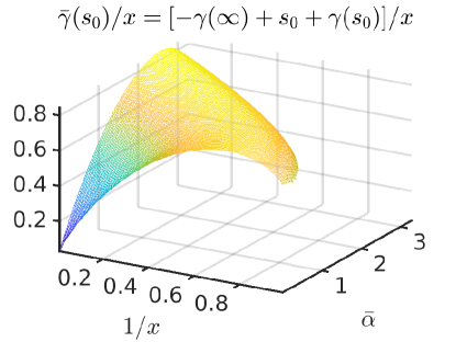
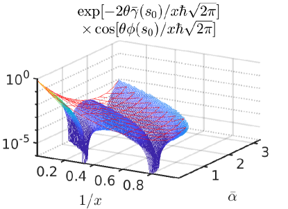
Figure 18: This figure shows exponential modulation of the survival probability, which is defined by an imaginary part of integrals over the energy split in complex plane, $\bar{\gamma}(s_{0})$, see text for details. The first panel shows the exponent, while the second panel shows the exponential modulation of the basic oscillatory term, which is associated with residua contributions, see Fig. 17. The pulse area $\theta=4\pi$.

13.1.2 Odd layout

The survival probability $p_{1}$ for the odd layout is obtained by analogy by using $v_{0}$ defined in Eqs. 370 and 372 such that

$$p_{1,odd}=f^{2}|v_{0,odd}|^{2}=f^{2}\frac{\pi^{2}}{9}e^{-\frac{\tau\Gamma}{\hbar}\left[\gamma(s_{0i})\right]}.$$ (382)

Using the definition of the pulse area in Eq. 305 and using the same definition for the normalization factor $f$ as in the previous case, we get

$$p_{1,odd}=\frac{\pi^{2}}{9}\exp\left[-\frac{2\,\theta}{\hbar\sqrt{2\pi}}\frac{\bar{\gamma}(s_{0i})}{x}\right].$$ (383)

We can see that in the case of odd layout, the oscillatory behavior is not present. The exponential decay is controlled by the effective integral $\bar{\gamma}(s_{0i})$ which is formally defined by the same equation as before, Eq. 379. The important conclusion following from here is that the odd layout of TPs in the complex plane of adiabatic time defines a monotonic subspace in the plane of the reduced laser parameters $x,{\bar{\alpha}}$.

13.1.3 Comparison with a numerical calculation

We demonstrate results obtained using the analytical formulas Eqs. 381 and 383 in comparison with a numerically implemented first order perturbation method based on the integration along the real time axis as given in Eq. 283. The comparison is presented in Fig. 19. The agreement is remarkable even for the relatively small pulse areas $\theta\in\{4\pi,6\pi\}$, showing some improvement as the pulse area gets larger. This favorable result shows that the complex time plane method can be recomended as an analytical tool for different problems concerning the EP encircling dynamics.

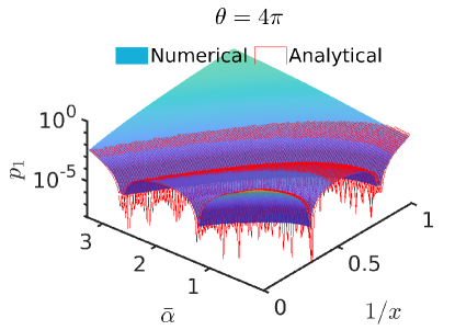
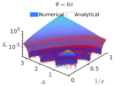
Figure 19: The results on these figures showing the survival probability have been obtained using the analytical formula Eq. 377, which is applicable for the oscillatory subspace of the laser parameters $[x,{\bar{\alpha}}]$, and the numerical first order perturbation method, Eq. 283. The analytical formula derived for the limiting pulse length area $\theta\to\infty$ is tested for two finite values of $\theta\in\{4\pi,6\pi\}$.

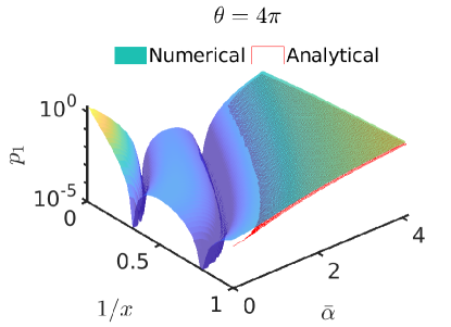
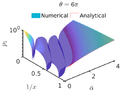
Figure 20: The results on these figures showing the survival probability have been obtained using the analytical formula Eq. 383, which is applicable for the non-oscillatory subspace of the laser parameters $[x,{\bar{\alpha}}]$, and the numerical first order perturbation method, Eq. 283. The analytical formula derived for the limiting pulse length area $\theta\to\infty$ is tested for two finite values of $\theta\in\{4\pi,6\pi\}$.

13.1.4 Survival probability at the separator crossing

Let us add a very short comment on the crossing over the separator. Eqs. 381 and 383 show a discontinuity that should appear on the survival probability. To study this, we performed a comparison of the analytical results with the numerical solution of first-order adiabatic perturbation theory which are summarized in Appendix K. The abrupt change of the prefactor seems to be a specific property of the large pulse area limit. More importantly, the amplitude of the survival probability decays exponentially at the crossing of the separator, which overloads the changes of the prefactor at least in the overall picture.

13.2 Analytical fit for the functions defining the survival probability

The functions $\bar{\gamma}[s_{0}(\varepsilon_{0},{\bar{\alpha}})]/x$ and $\phi[s_{0}(\varepsilon_{0},{\bar{\alpha}})]/x$ (displayed in Figs. 17 and 18) control the very behavior of the survival probability. These functions must be obtained numerically through evaluation of the residua at the cental TPs, which is not very convenient. It is therefore beneficial, in the view of possible future applications, to have analytical expressions for the functions $\bar{\gamma}[s_{0}(\varepsilon_{0},{\bar{\alpha}})]/x$ and $\phi[s_{0}(\varepsilon_{0},{\bar{\alpha}})]/x$ which would be based on a suitable fit to the numerically obtained values.

13.2.1 Natural coordinates on the laser pulse parameter plane

For the sake of convenience we define the plane displayed in Figs. 17 and 18 using new defined coordinates $X$ and $Y$ such that

$$X=\frac{1}{\bar{\varepsilon}_{0}}, Y=\frac{{\bar{\alpha}}}{2\sqrt{e}}.$$ (384)

Note that the oscillations associated with the even layout of the TPs take place within the interval

$$0\leq X\leq 1, 0\leq Y\leq 1.$$ (385)

As a matter of fact, the functions $\bar{\gamma}(1/\varepsilon_{0},{\bar{\alpha}}/2\sqrt{e})/x$ and $\phi(1/\varepsilon_{0},{\bar{\alpha}}/2\sqrt{e})/x$ are almost radial, namely we can hardly see any angular dependence in Figs. 17 or 18. We define $\varphi$ as the angle of the plane and $\eta$ as a decreasing function with $\varphi$:

$$\varphi=\arctan\frac{X}{Y}\ ,$$ (386)

$$\eta=\frac{1}{2\sqrt{e}}\left(\sqrt{\left(\frac{X}{Y}\right)^{2}+4e\,}\,-\,\frac{X}{Y}\right)\,,$$ (387)

and a convenient “radius” $R$ such that

$$R=e^{-\eta^{2}/2}\cdot\left(Y\,\sqrt{e}\ \eta+X\right)\,.$$ (388)

This choice of $R$ is in fact based on the definition of the separator $s$ displayed in Fig. 5, which is the solution of Eq. 139 when using Eq. 143. Namely, we get the separator of the plane for $R=1$; for $R<1$ we get the oscillatory regime (even layout of TPs), for $R>1$ we get the monotonic regime (odd layout of TPs).

13.2.2 Fit of $\phi/x$ defining Rabi oscillations

The behavior of $\phi/x$ is roughly linear in $R$ and independent of $\varphi$,

$$\frac{\phi}{x}\approx-\sqrt{\frac{\pi}{2}}(1-R).$$ (389)

To provide a precision fit, we use a quartic polynomial for the $R$ dependence, adding a mild angular dependence $f(\varphi,R)$, such that

$$\frac{\phi}{x}=\left(-\sqrt{\frac{\pi}{2}}+\sum\limits_{k=1}^{4}a_{k}R^{k}\right)+f(\varphi,R),$$ (390)

where

$$a_{1}=0.6428,\quad a_{2}=1.5637,$$ (391)

$$a_{3}=-1.4929,\quad a_{4}=0.5398.$$ (392)

Note that the sum over the polynomial coefficients is equal zero,

$$\sum\limits_{k=1}^{4}a_{k}=0.$$ (393)

The mild angular dependence $f$ is fitted to the analytical expression

$$f=g(\varphi)\cdot\sin\left[\pi(R+\delta_{R})\right],$$ (394)

$$g=b_{0}\ \left[\left(1-\frac{2\varphi}{\pi}\right)^{3}+\left(\frac{b_{1}}{b_{0}}\right)^{3}\right]^{1/3},$$ (395)

$$\delta_{R}=8c_{0}\,\frac{\varphi}{\pi}\ R\,(R-1),$$ (396)

where

$$b_{0}=0.1093,\quad b_{1}=0.03569,$$ (397)

$$c_{0}=0.0912.$$ (398)

Note that

$$f(\varphi,R=0)=f(\varphi,R=1)=0.$$ (399)

The maximum error of this fit is given by $10^{-4}$.

13.2.3 Fit of $\bar{\gamma}/x$ defining exponential damping of the survival probability

Also the character of $\bar{\gamma}/x$ is determined by the $R$-dependence, whereas the angular dependence is minor, see Fig. 18.

Via a numerical inspection of the dependence of $\bar{\gamma}/x$ on $R$ we discovered a very specific analytical behavior at the criticality, $R=1$. The found analytical form of $\bar{\gamma}/x$ is given by,

$$\frac{\bar{\gamma}}{x}\ =\ a_{0}\ +$$ (400)

$$\quad f_{\pm}\cdot\ln|R-1|\cdot\tan[2\arctan(R-1)],$$ (401)

where $f_{+}$ and $f_{-}$ represent two different functions. $f_{+}$ is applicable in the interval $1<R<2$ and is approximately linear. $f_{-}$ is applicable for $0<R<1$ and is approximately parabolic.

To achieve a satisfactory precision, however, $f_{-}$ is fitted to a fifth order polynomial in $(R-1)$ and second order polynomial is used to define the angular dependence of the polynomial coefficients:

$$f_{-}(R,\varphi)=\sum\limits_{k=0}^{5}\sum\limits_{l=0}^{2}c^{-}_{k,l}\ \varphi^{l}\cdot(R-1)^{k}.$$ (403)

The coefficients $c^{-}_{k,l}$ are listed in Table 1. $f_{+}$ is fitted to a second order polynomial to get the radial dependence, and a third order polynomial to get the angular dependence:

$$f_{+}(R,\varphi)=\sum\limits_{k=0}^{2}\sum\limits_{l=0}^{3}c^{+}_{k,l}\ \varphi^{l}\cdot(R-1)^{k}.$$ (404)

The coefficients $c^{+}_{k,l}$ are listed in Table 2. $a_{0}$ is fitted to a second order polynomial to get its angular dependence:

$$a_{0}=0.0207\ \varphi^{2}-0.0585\ \varphi+0.685.$$ (405)

Finally, the asymptotic behavior of $\bar{\gamma}/x$ for $R>2$ does not fit well to the form of Eq. LABEL:EQFitC. Instead, we use the racional form,

$$\frac{\bar{\gamma}}{x}\ =\frac{1}{\sum\limits_{k=0}^{2}\sum\limits_{l=0}^{2}c^{\infty}_{k,l}\ \varphi^{l}\cdot(R-1)^{k}},$$ (406)

where the coefficients $c^{\infty}_{k,l}$ are listed in Table 3.

The maximum error of this analytical fit for $\bar{\gamma}/x$ on the covered interval ($R<5$) is given by $0.0035$ (near $R=0$), whereas the standard deviation calculated for the errors is given by $0.0007$.

$c^{-}_{k,l}$	$l=2$	$l=1$	$l=0$
$k=5$	-0.399	0.996	0.315
$k=4$	-0.893	2.14	0.476
$k=3$	-0.779	1.79	0.358
$k=2$	-0.343	0.763	-0.641
$k=1$	-0.0306	0.0341	0.133
$k=0$	0.00384	-0.0171	0.288

Table 1: Expansion coefficients for $f_{-}$, which codefines the analytical fit for $\bar{\gamma}/x$ near the critical behavior, $0<R<1$, see Eq. 406 and equations below.

$c^{+}_{k,l}$	$l=3$	$l=2$	$l=1$	$l=0$
$k=2$	0.02704	-0.05689	0.02424	-0.007911
$k=1$	-0.03046	0.06553	-0.0293	0.1553
$k=0$	0.004964	-0.0007442	-0.0229	0.2883

Table 2: Expansion coefficients for $f_{+}$, which codefines the analytical fit for $\bar{\gamma}/x$ near the critical behavior, $1<R<2$, see Eq. LABEL:EQFitC and equations below.

$c^{\infty}_{k,l}$	$l=2$	$l=1$	$l=0$
$k=2$	-0.495	0.382	-0.0106
$k=1$	0.559	0.107	2.16
$k=0$	-0.319	0.137	1.82

Table 3: Expansion coefficients for the analytical fit for $\bar{\gamma}/x$ at the asymptotic distances $R>2$, see Eq. LABEL:EQFitC and equations below.

14 Conclusions

We have adjusted the complex time plane method (discovered originally by Dykhne, David, and Pechukas) to study non-Hermitian quantum dynamics where an exceptional point is encircled. To do this we proposed a new integration contour for non-Hermitian problems.

The key idea of the complex time plane method is based on the fact that the quasi-energy split as a function of adiabatic time can be decomposed as a product first-order Puiseux expansion which is based on branchpoints in the complex time plane. These branchpoints have the same properties as exceptional points up to the fact that they occur in the complex time plane rather then a plane defined by physical parameters. (The term TPs goes back to the research of non-adiabatic jumps at avoided crossings of potential curves in the scattering theory.)

The complex amplitude of the quantum states in the end of the encircling loop is expressed via a sum of contributions associated with all individual TPs. We derived analytical expressions for these contributions which are valid in the semiclassical limit here characterized by the large pulse area. Each TP contribution consists of two different additive terms given by Eqs. 335 and 309, which reflect separate residual and branchcut contributions of such singularities, respectively.

The currect study is limited to solution within the first order perturbation theory and to the problem of the survival amplitude if only one state is initially populated under the additional condition that this state is the less dissipative one. An improvement and generalization of the complex time method beyond this approximation and to other cases remains an open problem at this point.

We illustrate the application of the complex time method in its present form for the special case where the encircling dynamics is time symmetric, namely the time-asymmetric mode switching does not take place. This case is new and therefore carefully introduced. The time-symmetric EP encircling is associated with a new phenomenon which is represented by a behavior switch between Rabi oscillations and rapid adiabatic passage. We discuss that this phenomenon is associated with a coalescence of two TPs of the first Puiseux order upon a formation of one TP of the second Puiseux order.

Appendix A Derivation of rotating wave approximation (RWA)

A.1 Classical dipole approximation

We start from the classical dipole approximation. The Hamiltonian for the driven atom is given by,

$$\hat{H}(t)=\hat{H}_{0}+\hat{V}_{int}(t),$$ (407)

where $\hat{H}_{0}$ is the Hamiltonian for the field free atom and $\hat{V}_{int}(t)$ is the interaction term. We use the length gauge where

$$\hat{V}_{int}(t)=\left(\sum\limits_{k=1}^{N_{el}}\hat{x}_{k}\right)\varepsilon_{0}(t)\,\cos\left[\omega(t)t\right].$$ (408)

A.2 Floquet Hamiltonian as a foundation for an adiabatic ansatz

Given the fact that the pulse hosts many optical cycles,

$$\tau\gg\frac{2\pi}{\omega_{r}},$$ (409)

it is possible to separate the fast and slow time coordinates in the field interaction term $V_{int}(t)$, Eq. 99 and 100, where the fast variation is represented by the field oscillations given by the cosine term, while the slow variation is represented by the change of the pulse strength $\varepsilon_{0}(t)$ and frequency $\omega(t)$. Based on this reasoning we define the instantaneous states $\Phi[{\boldsymbol{r}},t^{\prime};\omega(t),\varepsilon_{0}(t)]$ of the driven atom in the continuous wave (CW) field corresponding to the given instantaneous frequency and strength, $[\omega(t),\varepsilon_{0}(t)]$, where $t^{\prime}$ is here the fast coordinate, while $t$ is here assumed only as a parameter of the slow coordinate. Such states are defined as the solutions of the Floquet Hamiltonian,

$$\left\{\hat{H}_{0}+\hat{V}_{int-cw}[t^{\prime};\omega(t),\varepsilon_{0}(t)]-i\hbar\frac{\partial}{\partial t^{\prime}}\right\}$$ (410)

$$\times\quad\Phi[{\boldsymbol{r}},t^{\prime};\omega(t),\varepsilon_{0}(t)]$$ (411)

$$\quad=\epsilon_{k}[\omega(t),\varepsilon_{0}(t)]\Phi[{\boldsymbol{r}},t^{\prime};\omega(t),\varepsilon_{0}(t)],$$ (412)

where $\epsilon_{k}$ are the Floquet energies (quasienergies), which depend on the instantaneous parameters $[\omega(t),\varepsilon_{0}(t)]$. The interaction term in the length gauge is given correspondingly to Eq. 408 as

$$\hat{V}_{int-cw}[t^{\prime};\omega(t),\varepsilon_{0}(t)]=\left(\sum\limits_{k=1}^{N_{el}}\hat{x}_{k}\right)\varepsilon_{0}(t)\,\cos\left[\omega(t)t^{\prime}\right].$$ (413)

The Floquet Hamiltonian is expanded in the basis set of the field free atomic states $\psi_{k}$,

$$\hat{H}_{0}\psi_{k}={\cal E}_{k}\psi_{k},$$ (414)

and Fourier components $\exp(in\omega t^{\prime})$:

$$\left[\begin{matrix}&&&\dots&&&\\ &{\boldsymbol{{\cal E}}}-2\hbar\omega&\frac{\varepsilon_{0}}{2}{\boldsymbol{\mu}}&{\boldsymbol{0}}&{\boldsymbol{0}}&{\boldsymbol{0}}&\\ &\frac{\varepsilon_{0}}{2}{\boldsymbol{\mu}}&{\boldsymbol{{\cal E}}}-\hbar\omega&\frac{\varepsilon_{0}}{2}{\boldsymbol{\mu}}&{\boldsymbol{0}}&{\boldsymbol{0}}&\\ \dots&{\boldsymbol{0}}&\frac{\varepsilon_{0}}{2}{\boldsymbol{\mu}}&{\boldsymbol{E}}&\frac{\varepsilon_{0}}{2}{\boldsymbol{\mu}}&{\boldsymbol{0}}&\dots\\ &{\boldsymbol{0}}&{\boldsymbol{0}}&\frac{\varepsilon_{0}}{2}{\boldsymbol{\mu}}&{\boldsymbol{{\cal E}}}+\hbar\omega&\frac{\varepsilon_{0}}{2}{\boldsymbol{\mu}}&\\ &{\boldsymbol{0}}&{\boldsymbol{0}}&{\boldsymbol{0}}&\frac{\varepsilon_{0}}{2}{\boldsymbol{\mu}}&{\boldsymbol{{\cal E}}}+2\hbar\omega&\\ &&&\dots&&&\\ \end{matrix}\right],$$ (415)

where ${\boldsymbol{{\cal E}}}$ is the diagonal matrix of the field free atomic energies,

$${\boldsymbol{{\cal E}}}=\left[\begin{matrix}{\cal E}_{1}&0&\\ 0&{\cal E}_{2}&\\ &&\dots\\ \end{matrix}\right],$$ (416)

and ${\boldsymbol{\mu}}$ is the corresponding matrix of the transition dipole operator in the basis set of the field free atomic states,

$$\{{\boldsymbol{\mu}}\}_{i,j}=(\psi_{i}^{(l)}|\sum\limits_{k=1}^{N_{el}}\hat{x}_{k}\left|\psi_{j}\right),$$ (417)

where $\psi_{i}^{(l)}$ represents the left vector as solution of the transposed Hamiltonian operator, $\hat{H}_{0}^{t}$.

A.3 Rotating wave approximation

The rotating wave approximation (RWA) represents an approximation to the pair of Floquet states, which correspond to two atomic states coupled by a foton tuned near their resonance frequency. It is valid when the coupling elements $\varepsilon_{0}{\boldsymbol{\mu}}/2$ are relatively small, therefore the coupling to other atomic states and higher Fourier components (multifoton processes) is negligible. The Floquet operator for these two strongly coupled Floquet vectors simplifies as,

$$\left[\begin{matrix}{\cal E}_{2}&\frac{\varepsilon_{0}}{2}\mu_{2,1}\\ \frac{\varepsilon_{0}}{2}\mu_{1,2}&{\cal E}_{1}+\hbar\omega\end{matrix}\right]+n\hbar\omega\left[\begin{matrix}1&0\\ 0&1\end{matrix}\right],$$ (418)

where $n$ represents the shift of the Brillouine zone. The Floquet vectors in different Brillouine zones are equivalent up to the phase shift $e^{in\omega t^{\prime}}$, therefore only one pair of the Floquet vectors needs to be calculated. In this vector pair we may also exclude the phase factor $e^{-iE_{2}t^{\prime}/\hbar}$, which leads to the usual form of the RWA Hamiltonian given by,

$$\hbar\left[\begin{matrix}0&\frac{1}{2}\Omega\\ \frac{1}{2}\Omega&\Delta\end{matrix}\right],$$ (419)

where

$$\Delta=\omega-({\cal E}_{2}-{\cal E}_{1})/\hbar$$ (420)

is the frequency detuning, which may be generally complex if ${\cal E}_{1}$ or ${\cal E}_{2}$ are complex, and

$$\Omega=\mu_{1,2}\varepsilon_{0}/\hbar$$ (421)

is the Rabi frequency, where $\mu_{1,2}$ is the transition dipole element between states $|1\rangle$ and $|2\rangle$. Note that this form of Hamiltonian is widely used in quantum optics. This Floquet Hamiltonian can be precisely written as

$$\hat{H}_{F}=\hat{H}_{0}+\hat{V}_{int-cw}[t^{\prime};\omega(t),\varepsilon_{0}(t)]-i\hbar\frac{\partial}{\partial t^{\prime}}$$ (422)

$$\approx|e^{i\omega t^{\prime}}e^{iE_{2}t^{\prime}/\hbar}\psi_{1})(e^{-i\omega t^{\prime}}e^{-iE_{2}t^{\prime}/\hbar}\psi_{1}^{(l)}|\hbar\Delta(t)+$$ (423)

$$\quad+\frac{\hbar\Omega(t)}{2}\bigg{[}|e^{i\omega t^{\prime}}e^{iE_{2}t^{\prime}/\hbar}\psi_{1})(e^{-iE_{2}t^{\prime}/\hbar}\psi_{2}^{(l)}|+$$ (424)

$$\quad|\psi_{2}e^{iE_{2}t^{\prime}/\hbar})(e^{i\omega t^{\prime}}e^{-iE_{2}t^{\prime}/\hbar}\psi_{1}^{(l)}|\bigg{]}+\cdots,$$ (425)

where the dots represent the other Brillouine zones and the dressed atomic states, which nearly do not interact with each other nor the coupled pair of states.

Let us apply the RWA to our problem. The detuning can be rewritten using the definition of energies of the relevant field free states $|1\rangle$ and $|2\rangle$ defined in Section 2.1

$${\cal E}_{1}=E_{1}, {\cal E}_{2}=E_{2}-i\Gamma/2,$$ (426)

such that

$$\Delta=\omega-[(E_{2}-i\Gamma/2)-E_{1}]/\hbar=\omega-\omega_{r}+\frac{i\Gamma}{2\hbar},$$ (427)

where we used the resonance frequency $\omega_{r}$ defined in Eq. 8. We will also simplify the notation of the transition dipole element between the two field-free states – Appendix B – such that

$$\mu=\mu_{1,2}=\mu_{2,1}.$$ (428)

By using this notation we rewrite the definition of the Rabi frequency such that

$$\Omega=\mu\,\varepsilon_{0}/\hbar.$$ (429)

Appendix B Transition dipole element

The transition dipole moment $\mu_{1,2}$ is directly related to the oscillator strength $f_{1\to 2}$ of the transition $|1\rangle\to|2\rangle$ through the relation

$$|\mu_{1,2}|^{2}=f_{1\to 2}\cdot\frac{3\hbar d}{2m_{e}\omega_{r}},$$ (430)

where $d$ represents a factor taking care for the rotational degeneracies of the atomic levels, $d=\max(L_{1},L_{2})/(2L_{2}+1)$, where $L_{1},L_{2}$ are the main rotational numbers of the initial and excited states, respectively.

The transition dipole moment which couples non-Hermitian resonance states to bound states may acquire complex values in general. However, here we restrict ourselves to transitions which are characterized by approximately real defined transition dipole elements:

$$\mu_{1,2}\in\Re\ .$$ (431)

Note that a relation between the complex phase of the transition dipole element and asymmetric absorption lines exists as discussed in Ref. [48].

Appendix C Instantaneous adiabatic states

The instantaneous adiabatic states are defined based on the solution of the time-dependent Schrödinger equation,

$$i\hbar\frac{\partial}{\partial t^{\prime}}\psi[{\boldsymbol{r}},t^{\prime};\omega(t),\varepsilon_{0}(t)]=$$ (432)

$$\quad\left\{\hat{H}_{0}+\hat{V}_{int-cw}[t^{\prime};\omega(t),\varepsilon_{0}(t)]\right\}$$ (433)

$$\times\quad\psi[{\boldsymbol{r}},t^{\prime};\omega(t),\varepsilon_{0}(t)],$$ (434)

where the time evolution is performed considering only the fast field oscillations as a part of the interaction Hamiltonian (the fast time is denoted as $t^{\prime}$), while the slowly varying instantaneous frequency $\omega(t)$ and laser strength $\varepsilon_{0}(t)$ are considered as constant parameters. It is required that each of the solutions corresponds to only one Floquet state, such that

$$\psi_{\pm}[{\boldsymbol{r}},t^{\prime};\omega(t),\varepsilon_{0}(t)]=e^{-\frac{i}{\hbar}\epsilon_{\pm}(t)t^{\prime}}\ \Phi_{\pm}[{\boldsymbol{r}},t^{\prime};\omega(t),\varepsilon_{0}(t)].$$ (435)

The instantaneous adiabatic states $\psi_{ad,\pm}$ are defined as an approximation to the solutions of the time-dependent Schrödinger equation, where the two time-scales are not divided,

$$i\hbar\frac{\partial}{\partial t}\psi_{ad}({\boldsymbol{r}},t)\approx$$ (436)

$$\left\{\hat{H}_{0}+\hat{V}_{int-cw}[t;\omega(t),\varepsilon_{0}(t)]\right\}\psi_{ad}({\boldsymbol{r}},t),$$ (437)

using the solutions including only the fast time coordinate $\psi_{\pm}$, and assuming that the slow time coordinate does not cause any mixing of the Floquet states such that,

$$\psi_{ad,\pm}({\boldsymbol{r}},t)=e^{-\frac{i}{\hbar}\int\limits_{0}^{t}dt^{\prime}\,\epsilon_{\pm}(t^{\prime})}\ \Phi_{\pm}[{\boldsymbol{r}},t;\omega(t),\varepsilon_{0}(t)].$$ (438)

Appendix D Numerical verification of the convergence of adiabatic perturbation theory in the case of Gaussian chirped pulses

In this Section, we demonstrate the convergence of the perturbation series for the amplitude $a_{+}$ given in Eqs. 82 and 84 numerically. We evaluated the perturbation series for the case of a linearly chirped Gaussian pulse using the analytical definitions for quasienergy split (Eq. 122, see also Section 6.2 concerning the sign of the quasienergy split) and non-adiabatic coupling (see Appendix F.1, Eq. 459). The values of the perturbation corrections after the pulse is over (at $s\to\infty$) are denoted as

$$v_{j}\equiv\bar{v}^{(j)}(s\to\infty).$$ (439)

The quantities $v_{j}$ are dependent on the laser parameters $x$ (corresponding with the peak pulse strength, Eq. 119), ${\bar{\alpha}}$ (the effective pulse chirp, Eq. 120), and $\theta$ (the pulse area, Eq. 113);

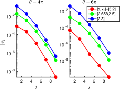
Figure 21: Convergence of the perturbation series in the whole range of studied laser parameters is demonstrated. The amplitude $a_{+}$ of the field-free bound state after the pulse is over is calculated using an infinite perturbation series, Eq. 82 where $s\to\infty$. Contributions of $|v_{j}|$, where $j$ is the perturbation order, have been obtained by a numerical evaluation of Eq. 84 for different pulse parameters here defined by $x$, ${\bar{\alpha}}$, and $\theta$ (see text).

We performed numerical calculations for three different sets of pulse parameters ($x$, ${\bar{\alpha}}$, $\tau$), which are relevant to the studied phenomenon, where the choice of the concrete values of $x$ and ${\bar{\alpha}}$ taken in the calculations has been $[x,{\bar{\alpha}}]=\{[5,2],\ [2.658,2.5],\ [2,3]$. The convergence is logarithmic with the perturbation order, see Fig. 21, which provides an evidence that the perturbation series is convergent. The speed of convergence (the ratio between the subsequent orders) is raughly independent of the pulse area $\theta$ in the regime where the studied phenomenon appears, i.e. $\theta$ is sufficently large ($\theta>4$).

Appendix E Derivation of asymptotic series of transition points

We start our derivation from the approximate Eq. 144. For the subsequent TP $s_{k+1}$ we can write the same equation

$$e^{-s_{k+1}^{2}}=-\left(\frac{{\bar{\alpha}}}{2}\right)^{2}s_{k+1}^{2}.$$ (440)

Now we define the difference

$$\xi=s_{k+1}^{2}-s_{k}^{2}$$ (441)

and substitute to Eq. 440 such that

$$e^{-s_{k}^{2}}e^{-\xi}=-\left(\frac{{\bar{\alpha}}}{2}\right)^{2}(s_{k}^{2}+\xi).$$ (442)

If we make the assumption that $\xi$ is a finite number in the asymptotic limit $|s_{k}|\to\infty$, then $\xi$ can be neglected on the right hand side of Eq. 442:

$$e^{-s_{k}^{2}}e^{-\xi}=-\left(\frac{{\bar{\alpha}}}{2}\right)^{2}s_{k}^{2}.$$ (443)

By substituting from Eq. 144 we get

$$e^{-\xi}=1$$ (444)

and from here

$$\xi=\pm 2i\pi.$$ (445)

Because $\xi$ does not depend on index $k$ for the asymptotic limit $|s_{k}|\to\infty$, we see that $s_{k}^{2}$ take the form of the linear series in this limit such that,

$$s_{k}^{2}=k\cdot 2i\pi+c,$$ (446)

where $c$ is an unknown complex constant. Let us take a logarithm from Eq. 144:

$$s_{k}^{2}=-\ln(-)-2\ln\frac{{\bar{\alpha}}}{2}-\ln s_{k}^{2}+k^{\prime}\cdot 2i\pi,$$ (447)

where we add an arbitrary multiplier of $k^{\prime}\cdot 2i\pi$. Now we substitute for the asymptotic series from Eq. 446:

$$c=(k^{\prime}-k)\cdot 2i\pi-\ln(-)-2\ln\frac{{\bar{\alpha}}}{2}-\ln(k\cdot 2i\pi+c)$$ (448)

and we take the limit $k\to\infty$:

$$c=(k^{\prime}-k)\cdot 2i\pi-i\pi-2\ln\frac{{\bar{\alpha}}}{2}-\ln(k\cdot 2i\pi)$$ (449)

and separate the logarithm of imaginary unit:

$$c=(k^{\prime}-k)\cdot 2i\pi-i\pi-2\ln\frac{{\bar{\alpha}}}{2}-\ln(2k\pi)-\ln i$$ (450)

$$\quad\quad=(k^{\prime}-k)\cdot 2i\pi-3i\pi/2-2\ln\frac{{\bar{\alpha}}}{2}-\ln(2k\pi).$$ (451)

Because the choice of $k^{\prime}$ is arbitrary one may write

$$c=i\pi/2-\ln(2k\pi)-2\ln\left(\frac{{\bar{\alpha}}}{2}\right).$$ (452)

From here we get

$$s_{k}^{2}=k\cdot 2i\pi+i\pi/2-\ln(2k\pi)-2\ln\left(\frac{{\bar{\alpha}}}{2}\right),$$ (453)

$$\quad k\to\infty.$$ (454)

Appendix F Various expressions for non-adiabatic coupling term

F.1 Non-adiabatic coupling element for linear Gaussian chirp

The non-adiabatic coupling element $\bar{N}(s)$ is defined in Eq. 117, which can be also written as

$$\bar{N}(s)=\frac{1}{2}\frac{d\bar{\lambda}(s)}{ds}\left(\frac{1}{1+i\bar{\lambda}(s)}+\frac{1}{1-i\bar{\lambda}(s)}\right).$$ (455)

Using the definition of $\bar{\lambda}(s)$ within Eqs. 122,

$$\bar{\lambda}(s)=e^{s^{2}/2}\cdot\left(\frac{\bar{\alpha}}{2}\,s+\frac{i}{x}\right),$$ (122 revisited)

we get

$$\frac{d\bar{\lambda}}{ds}=\left[\frac{{\bar{\alpha}}}{2}(s^{2}+1)+\frac{i}{x}s\right]e^{s^{2}/2}.$$ (456)

Using the definition of $\bar{\lambda}$ in Eq. 122 we get also

$$\frac{1}{i\pm\frac{\Delta}{\Omega}}=\frac{1}{i\pm\left(\frac{{\bar{\alpha}}}{2}s+\frac{i}{x}\right)e^{s^{2}/2}}.$$ (457)

From here,

$$\bar{N}(s)=\frac{(s^{2}+1)+i\frac{2}{{\bar{\alpha}}x}s}{4}$$ (458)

$$\times\quad\sum\limits_{z=\{+/-\}}\frac{z}{\left(is-\frac{2}{{\bar{\alpha}}x}\right)-z\frac{2}{{\bar{\alpha}}}e^{-s^{2}/2}}.$$ (459)

F.2 First-order expansion of the non-adiabatic coupling term near the poles

We will start from the definition of the non-adiabatic coupling element for the linearly chirped Gaussian pulse given in Eq. 459. Let us denote $\xi=s-s_{k}$ a small distance from the EP $s_{k}$ in the complex plane of $s$ and substitute to the above equation:

$$\bar{N}(s)=\frac{s_{k}^{2}+2\xi\left(s_{k}+\frac{i}{{\bar{\alpha}}x}\right)+\left(1+\frac{2is_{k}}{{\bar{\alpha}}x}\right)}{4}$$ (460)

$$\times\sum\limits_{z=\{+/-\}}\frac{z}{i(s_{k}+\xi)-\frac{2}{{\bar{\alpha}}x}-z\frac{2}{{\bar{\alpha}}}e^{-s_{k}^{2}/2}e^{-s_{k}\xi}},$$ (461)

where we neglected the second-order terms $\xi^{2}$ in the exponential, as it is assumed $\xi\to 0$. Additionally, we may neglect the term in the sum, which is not the pole. We may write,

$$\bar{N}(s)=\frac{s_{k}^{2}+2\xi\left(s_{k}+\frac{i}{{\bar{\alpha}}x}\right)+\left(1+\frac{2is_{k}}{{\bar{\alpha}}x}\right)}{4}$$ (462)

$$\times\frac{z_{k}}{i(s_{k}+\xi)-\frac{2}{{\bar{\alpha}}x}-z_{k}\frac{2}{{\bar{\alpha}}}e^{-s_{k}^{2}/2}e^{-s_{k}\xi}},$$ (463)

where $z_{k}$ is given by the condition,

$$is_{k}-z_{k}\frac{2}{{\bar{\alpha}}}e^{-s_{k}^{2}/2}-\frac{2}{{\bar{\alpha}}x}=0.$$ (464)

By substituting Eq. 464 to Eq. 463 we get

$$\bar{N}(s)=\frac{s_{k}^{2}+2\xi\left(s_{k}+\frac{i}{{\bar{\alpha}}x}\right)+\left(1+\frac{2is_{k}}{{\bar{\alpha}}x}\right)}{4}$$ (465)

$$\times\frac{z_{k}}{i(s_{k}+\xi)-\frac{2}{{\bar{\alpha}}x}+e^{-s_{k}\xi}\left(\frac{2}{{\bar{\alpha}}x}-is_{k}\right)},$$ (466)

Now we simplify the denominator by taking the limit $\xi\to 0$ for the exponential ($e^{-s_{k}\xi}\approx 1-s_{k}\xi$):

$$\bar{N}(s)=\frac{s_{k}^{2}+2\xi\left(s_{k}+\frac{i}{{\bar{\alpha}}x}\right)+\left(1+\frac{2is_{k}}{{\bar{\alpha}}x}\right)}{4}$$ (467)

$$\times\quad\frac{z_{k}}{i\xi\left(1+\frac{2is_{k}}{{\bar{\alpha}}x}+s_{k}^{2}\right)}.$$ (468)

Taking the limit $\xi\to 0$ also in the nominator allows us to simplify the expression for $\bar{N}(s)$ down to

$$\lim\limits_{s\to s_{k}}\bar{N}(s)=\frac{z_{k}}{4i\xi}=\frac{z_{k}}{4i(s-s_{k})}.$$ (469)

F.3 Asymptotic behavior of the non-adiabatic element

We start from the definition of the non-adiabatic coupling element given by Eq. 459. The asymptotic behavior for $|s|\to\infty$ is obtained if adding up the two terms in the sum such that

$$\bar{N}(s)=\frac{1}{{\bar{\alpha}}}\frac{(s^{2}+1)+i\frac{2}{{\bar{\alpha}}x}s}{\left(is-\frac{2}{{\bar{\alpha}}x}\right)^{2}\,e^{s^{2}/2}-\left(\frac{2}{{\bar{\alpha}}}\right)^{2}\,e^{-s^{2}/2}}.$$ (470)

If the real component of $s$ is larger then the imaginary component then the first term in the denominator prevails which yields,

$$|\arg s|<\pi/4\ or\ |\arg(-s)|<\pi/4:$$ (471)

$$\bar{N}(|s|\to\infty)=-\frac{1}{{\bar{\alpha}}}\,e^{-s^{2}/2},$$ (472)

while in the opposite case the second term in the denominator prevails which yields,

$$|\arg s|>\pi/4\ and\ |\arg(-s)|>\pi/4:$$ (473)

$$\bar{N}(|s|\to\infty)=-\frac{{\bar{\alpha}}}{4}\,s^{2}\,e^{s^{2}/2}.$$ (474)

In either case the non-adiabatic coupling exponentially quadratically decays to zero in all asymptotes. This behavior of the non-adiabatic coupling elements in the complex plane of time is demonstrated using a numerical evaluation in Fig. 8.

Appendix G Complex phase of local Puiseux coefficients for TPs based on linearly chirped Gaussian pulses

Let us analyze the complex phase for the local Puiseux coefficient $\beta_{k}^{(1)}$,

$$\beta_{k}^{(1)}=\sqrt{{\bar{\alpha}}\left(\frac{{\bar{\alpha}}}{2}s_{k}+\frac{i}{x}\right)-2s_{k}\,e^{-s_{k}^{2}}}$$ (206 revisited)

associated with the TP $s_{k}$ defined by

$$e^{-s_{k}^{2}}+\left(\frac{{\bar{\alpha}}}{2}s_{k}+\frac{i}{x}\right)^{2}=0.$$ (137 revisited)

G.1 TPs on the imaginary time axis

We will start for the case where the central TPs lie on the imaginary axis and we will use Eq. 137 to remove the exponential from the definition of $\beta_{k}^{(1)}$ such that

$$\beta_{k}^{(1)}=\sqrt{\left(\frac{{\bar{\alpha}}}{2}s_{k}+\frac{i}{x}\right)\,a},$$ (475)

$$a={\bar{\alpha}}+2s_{k}\left(\frac{{\bar{\alpha}}}{2}s_{k}+\frac{i}{x}\right).$$ (476)

$a$ is always real defined, having positive value for the lower TP and negative for the upper TP on the imaginary axis. Based on this fact the complex phases of the corresponding coefficients are given by,

$$\arg\beta_{0i,low}^{(1)}=\frac{3\pi}{4}\pm\frac{\pi}{2},$$ (477)

$$\arg\beta_{0i,upp}^{(1)}=\frac{\pi}{4}\pm\frac{\pi}{2}.$$ (478)

There are two possible values of the sign following from the square root. We know, however, that the sign has to fit with the definition of $(s-s_{k})^{1/2}$ in Fig. 9 and with the sign of $\tilde{\delta}(s)$ on the real time axis, $s\in\Re$. The lower TP $s_{0i,low}$ is very often very close to the real time axis, so that we may use this point to determine the correct sign. We assume that that the quasienergy split on the real time axis near the center, namely at the point $s=0$, can be written to a good approximation using the first order Puiseux expansion such that

$$\tilde{\delta}(s)\approx\beta_{0i,low}^{(1)}(s-s_{k})^{1/2}.$$ (479)

The phase of the square root is determined based on the rules explained in Fig. 9 such that

$$\arg(s-s_{k})\bigg{|}_{s=0}=\frac{3\pi}{2}$$ (480)

$$\rightarrow \arg(s-s_{k})^{1/2}\bigg{|}_{s=0}=\frac{3\pi}{4}.$$ (481)

The value of $\tilde{\delta}(s=0)$ is always purely real and positive, from where we know that its phase is given by zero, $\arg\tilde{\delta}(0)=0$. Using Eqs. 479 and 481 we determine the phase of the coefficient $\beta_{0i,low}^{(1)}$ such that

$$\arg\beta_{0i,low}^{(1)}=-\frac{3\pi}{4},$$ (482)

which is in accord with the upper definition given in Eqs. 478 derived independently for the general location of $s_{0i,low}$, not just near the real axis. Now, the sign uniquely derived as being $(+)$ for the specific case, can be generalized to any $s_{0i,low}$.

Now we aim to determine the unique sign of $\beta_{0i,upp}^{(1)}$ so far undetermined in the lower definition in Eq. 478. In order to do this we will study the case where the TPs $s_{0i,low}$ and $s_{0i,upp}$ are not far from their coalescence, see Section 6.4,

$$s_{0i,low}\approx s_{0i,upp}.$$ (483)

Based on Eq. 186, we can write the two corresponding local Puiseux expansion coefficients such that

$$\beta_{0i,low}^{(1)}=\alpha_{0i,low}\alpha_{0i,upp}(s_{0i,low}-s_{0i,upp})^{1/2}$$ (484)

$$\times\quad\prod\limits_{l\neq(0i)}\alpha_{l}(s_{0i,low}-s_{l})^{1/2}\quad,$$ (485)

$$\beta_{0i,upp}^{(1)}=\alpha_{0i,low}\alpha_{0i,upp}(s_{0i,upp}-s_{0i,low})^{1/2}$$ (486)

$$\times\quad\prod\limits_{l\neq(0i)}\alpha_{l}(s_{0i,upp}-s_{l})^{1/2}.$$ (487)

Not far from from coalescence, Eq. 483, the products concerning distant TPs can be considered equal,

$$f_{0}=\prod\limits_{l\neq(0i)}\alpha_{l}(s_{0i,low}-s_{l})^{1/2}$$ (488)

$$\quad\approx\prod\limits_{l\neq(0i)}\alpha_{l}(s_{0i,upp}-s_{l})^{1/2},$$ (489)

and

$$\beta_{0i,low}^{(1)}=\alpha_{0i,low}\alpha_{0i,upp}(s_{0i,low}-s_{0i,upp})^{1/2}\ f_{0},$$ (490)

$$\beta_{0i,upp}^{(1)}=\alpha_{0i,low}\alpha_{0i,upp}(s_{0i,upp}-s_{0i,low})^{1/2}\ f_{0}.$$ (491)

From here it follows that $\beta_{0i,low}^{(1)}$ and $\beta_{0i,upp}^{(1)}$ differ only in their phases near the coalescence. Now we need to determine the phase of the square roots including the complex vectors $(s_{0i,low}-s_{0i,upp})$ and $(s_{0i,upp}-s_{0i,low})$, respectively. It is possible to define the unique signs of the square roots based on Fig. 9, which is justified by the fact that the local Puiseux coefficients are defined based on Eq. 155 where $s$ has been replaced by the positions of the other TPs. By applying the rules given in Fig. 9 to the square roots in Eq. 491 we obtain

$$\arg(s_{0i,low}-s_{0i,upp})=-\frac{\pi}{2}$$ (492)

$$\quad\to\arg(s_{0i,low}-s_{0i,upp})^{1/2}=\frac{3\pi}{4},$$ (493)

$$\arg(s_{0i,upp}-s_{0i,low})=\frac{\pi}{2}$$ (494)

$$\quad\to\arg(s_{0i,up}-s_{0i,low})^{1/2}=\frac{\pi}{4},$$ (495)

from where we get

$$\beta_{0i,upp}^{(1)}=-i\ \beta_{0i,low}^{(1)},$$ (496)

which applies near the coalescence. The actual argument of $\beta_{0i,upp}^{(1)}$ near the coalescence is obtained using Eq. 482 derived above,

$$\arg\beta_{0i,upp}^{(1)}=-\frac{\pi}{4}.$$ (497)

This equation applies not only for the case when the TPs are near the coalescence, for which it has been derived. This special case helps us to determine the sign for the general definition of the phase in the second line of Eqs. 478, which implies that the phase Eq. 497 applies for the upper TP in general.

G.2 TPs near the coalescence

As the TPs lie on the imaginary time axis, the complex phases of their corresponding first order local Puiseux coefficients are defined by Eqs. 482 and 497. In the coalescence, the auxiliary variable $a$ defined in Eq. 476 is zero and very near to the coalescence, $a$ is infinitesimally small.

Let us define the TPs near the coalescence as

$$s_{k}=s_{coal}+\delta_{s}\ ,$$ (498)

where $s_{k}$ may stand for any TP near the coalescence,

$$s_{k}\in\{s_{0i,low},s_{0i,upp},s_{0},\bar{s}_{0}\}\ .$$ (499)

The auxiliary variable $a$ defined in Eq. 476 which measures how near is the coalescence of the TPs is expressed using $\delta_{s}$ such that

$$a=\ 2\,\delta_{s}\ \left(\bar{\alpha}s_{coal}+\frac{i}{x}\right)+\bar{\alpha}\,\delta_{s}^{2}\ .$$ (500)

We know that the coalescence always occurs on the positive imaginary time axis so that we can rewrite the above equation such that

$$a=\ 2i\,\delta_{s}\ \left(\bar{\alpha}|s_{coal}|+\frac{1}{x}\right)+\bar{\alpha}\,\delta_{s}^{2}\ .$$ (501)

As long as the TPs occur on the imaginary time axis, $\delta_{s}$ is an imaginary number and thus $a$ is real defined. On the other side of the coalescence, $\delta_{s}$ is a real defined small number. This implies that $a$ is an imaginary small number very near the coalescence,

$$\arg a(s_{0})=\frac{\pi}{2}, \arg a(\bar{s}_{0})=-\frac{\pi}{2},$$ (502)

$$s_{0}\approx\bar{s}_{0}\approx s_{coal}.$$ (503)

where the sign is defined by the sign of the variation $\delta_{s}$. The complex phase of the bracket below the square root in Eq. 476 is approximately given by $\pi/2$ as $\delta_{s}$ approximates to zero. Putting this together with the complex phase of $a$ we obtain the complex phases of $\beta_{0}^{(1)}$ and $\bar{\beta}_{0}^{(1)}$,

$$\arg\beta_{0}^{(1)}=\pm\frac{\pi}{2}, \arg\bar{\beta}_{0}^{(1)}=\frac{\pi}{2}\pm\frac{\pi}{2}.$$ (504)

The sign is determined using the fact that the quasienergy split is real and positive defined at the point $s=0$ on the real time axis. By studying the continuity of the quasienergy split on the imaginary time axis, using Eq. 138 and Fig. 5, we find out that the quasienergy split is also a positive define real defined number in the point of coalescence, $s=s_{coal}$, assuming that the coalescence occurs, and this would remain true also where the two TPs are near the coalescence, which is the case studied here. We express the quasienergy split at the point $s_{coal}$ using the general Puiseux expansion, Eq. 155, which includes the explicit contributions of the two near TPs $s_{0}$ and $\bar{s}_{0}$:

$$\tilde{\delta}(s_{coal})=\alpha_{0}{\bar{\alpha}}_{0}\sqrt{(s_{coal}-s_{0})(s_{coal}-\bar{s}_{0})}$$ (505)

$$\quad\times\quad\prod\limits_{k\neq 0}\alpha_{k}(s_{coal}-s_{k})^{1/2}.$$ (506)

Now we substitute the known the complex phases, where the phases of the square roots $(s_{coal}-s_{0})^{1/2}$ and $(s_{coal}-\bar{s}_{0})^{1/2}$ are determined based on the rules given in Fig. 9 assuming that the two complex vectors are perpendicular to the imaginary axis prior to the application of the square roots. We obtain,

$$\arg\tilde{\delta}(s_{coal}) =\arg\left(\alpha_{0}{\bar{\alpha}}_{0}\prod\limits_{k\neq 0}\alpha_{k}(s_{coal}-s_{k})^{1/2}\right)+\frac{\pi}{2}$$ (507)

$$=0.$$ (508)

Now we apply the definition of $\beta_{k}^{(1)}$ in Eqs. 186 to our case:

$$\beta_{0}^{(1)}=\alpha_{0}\bar{\alpha}_{0}(s_{0}-\bar{s}_{0})^{1/2}\prod\limits_{k\neq 0}\alpha_{k}(s_{0}-s_{k})^{1/2},$$ (509)

$$\bar{\beta}_{0}^{(1)}=\bar{\alpha}_{0}\alpha_{0}(\bar{s}_{0}-s_{0})^{1/2}\prod\limits_{k\neq 0}\alpha_{k}(\bar{s}_{0}-s_{k})^{1/2}.$$ (510)

The products over the higher TPs in the above equations can be simply approximated by using $s_{0}\approx\bar{s}_{0}\approx s_{coal}$ such that

$$\beta_{0}^{(1)}=f_{0}\,(s_{0}-\bar{s}_{0})^{1/2},$$ (511)

$$\bar{\beta}_{0}^{(1)}=f_{0}\,(\bar{s}_{0}-s_{0})^{1/2},$$ (512)

$$f_{0}=\alpha_{0}\bar{\alpha}_{0}\,\prod\limits_{k\neq 0}\alpha_{k}(s_{coal}-s_{k})^{1/2}\ .$$ (513)

In Eq. 508 we determined the complex phase of $f_{0}$ as $\arg f_{0}=-\pi/2$. The complex arguments of $(s_{0}-\bar{s}_{0})$ and $(\bar{s}_{0}-s_{0})$ are 0 and $\pi$, respectively, to which the square roots are applied based on Fig. 9. From here we get

$$\arg\beta_{0}^{(1)}=-\frac{\pi}{2}, \arg\bar{\beta}_{0}^{(1)}=0,$$ (514)

which is in accord with Eqs. 504.

G.3 Distant TPs

Let us analyze $\beta_{k}^{(1)}$ for the distant TPs. By applying the asymptotic limit for the TPs, see Section 6.6 and Eq. 144, we get the approximate value for $\beta_{k}^{(1)}$ given by,

$$\beta_{k\to\infty}^{(1)}=\pm\sqrt{\frac{{\bar{\alpha}}}{2}}\ s_{k}^{3/2}.$$ (515)

Let us determine the argument of this quantity. By taking the uppermost limit of $k\to\infty$ for $s_{k}$ using Eq. 149 we get

$$s_{k}\approx\sqrt{2i\pi k}=|\sqrt{2\pi k}|\cdot e^{i\pi/4}\,,$$ (516)

where we assume only the phase $\pi/4$ and not $-3\pi/4$ based on the fact that $s_{k}$ occurs in the upper imaginary half plane. Similarly we determine the limit of $\bar{s}_{k}$ as

$$\bar{s}_{k}\approx|\sqrt{2\pi k}|\cdot e^{3i\pi/4}\,.$$ (517)

The argument of $\beta_{k}^{(1)}$ based on Eqs. 515 and 516 is given by

$$\arg\beta_{k\to\infty}^{(1)}=\frac{3\pi}{8}-n\pi,\quad n\in\{0\cdots 1\},$$ (518)

and similarly the argument of $\bar{\beta}_{k}^{(1)}$ based on Eqs. 515 and 517 is given by

$$\arg\beta_{k\to\infty}^{(1)}=\frac{\pi}{8}-n\pi,\quad n\in\{0\cdots 1\}.$$ (519)

(a)
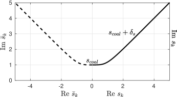
(b)
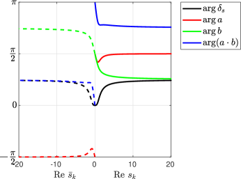
(c)

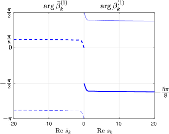
Figure 22: This figure shows how one can determine uniquely the complex phase of the local Puiseux coefficients $\beta_{k}^{(1)}$ and $\bar{\beta}_{k}^{(1)}$ for $k\to\infty$. (a) $s_{k}$ and $\bar{s}_{k}$ represent a specific pair of TPs, which we pursue as they move in the complex time-plane upon a continuous change of the laser parameters, starting at their coalescence ($k=0$) up to their joining the asymptotic limit ($k\to\infty$). (b) shows the complex phases of the variables $\delta_{s}$, $a$, and $b$, which are related to the positions of $s_{k}$ and $\bar{s}_{k}$, respectively. (c) shows the complex phases of the local Puiseux coefficients $\beta_{k}^{(1)}$ and $\bar{\beta}_{k}^{(1)}$ as related to the positions of the TPs $s_{k}$ and $\bar{s}_{k}$. As the Puiseux coefficients are related by the square root to the product $(a\cdot b)$, their correct signs (denoted by the thick lines) are determined based on the known values of the complex phases of $\beta_{0}^{(1)}$ and $\bar{\beta}_{0}^{(1)}$ near the coalescence of the TPs (which occurs for ${\rm Re}\,s_{0}=0$ and ${\rm Re}\,\bar{s}_{0}=0$, respectively).

We will solve the uncertainty of the sign due to the square root based on a heuristic reasoning using the continuity as the TPs $s_{0}$ and $\bar{s}_{0}$ defined near the coalescence, Eq. 498, move into the complex plane. We assume that the positions of $s_{0}$ and $\bar{s}_{0}$ are continually changed in the complex plane upon the variation of the laser parameters ${\bar{\alpha}}$ and $x$, such that they depart from $s_{coal}$ and penetrate deep to the complex plane. As this is happening, $\delta_{s}$ is increased, Eq. 498, first acquiring real values. Later, as the laser parameters are varied continually, $s_{0}$ and $\bar{s}_{0}$ penetrate yet deeper to the complex plane, while another pair of the TPs appears near the central part of the complex time plane. When this happens, the $k$ index of the monitored TPs is upgraded to $1$, such that $s_{0}\to s_{1}$, $\bar{s}_{0}\to\bar{s}_{1}$. $\delta_{s}$ is also no more a real number, as $s_{k}$ approaches the asymptotic limit $k\to\infty$ defined above. This process is shown in Fig. 22a.

The point of doing this reasoning is that we know the complex phase of $\beta_{0}^{(1)}$ and $\bar{\beta}_{0}^{(1)}$ near the coalescence (Eq. 514). The idea of continuity will navigate us to the right sign as $k$ is changed for a concrete pair of the TPs from $k=0$ to $k\to\infty$.

Let us now determine the phase of $a$ defined in Eq. 476 and $b$ which we define for the present purpose as

$$b=\frac{{\bar{\alpha}}}{2}s_{k}+\frac{i}{x},$$ (520)

where clearly

$$\beta_{k}^{(1)}=\sqrt{b\cdot a}.$$ (521)

Now, using the definition of $\delta_{s}$ in Eq. 498 and using 501

$$a=2i\delta_{s}\cdot A+{\bar{\alpha}}\delta_{s}^{2},$$ (522)

$$b=iB+\frac{{\bar{\alpha}}}{2}\delta_{s},$$ (523)

where $A$ and $B$ are real positive defined numbers. The evolution of the complex phase of $\delta_{s}$ corresponds with the trajectory of $s_{k}$, see Fig. 9a and  9b. The evolution of the complex phases of $a$ and $b$ can be raughly guessed if we substitute positive real numbers for $A$, $B$, and ${\bar{\alpha}}$, as shown in Fig. 9b. The complex phase of $\beta_{k}^{(1)}$ defined by the square root allows for the different sign, which we show in Fig. 9c and which is in agreement with our previous considerations, see Eqs. 518 and 519. Now, using the idea of continutity, the correct signs of $\beta_{k}^{(1)}$ and $\bar{\beta}_{k}^{(1)}$ may be determined from the known values for $\beta_{0}^{(1)}$ and $\bar{\beta}_{0}^{(1)}$, i.e. for ${\rm Re}s_{k}=0$, which are given in Eq. 514. As implied by Fig. 9c, the arguments of $\beta_{k}^{(1)}$ and $\bar{\beta}_{k}^{(1)}$ in the asymptotic limit are given by

$$\arg\beta_{k\to\infty}^{(1)}=-\frac{5\pi}{8}, \arg\bar{\beta}_{k\to\infty}^{(1)}=\frac{\pi}{8}.$$ (524)

Note that Eqs. 524 satisfy the symmetry relation given in Eq. 204.

Appendix H Analytical derivation of asymptotic expressions for the equivalue lines

H.1 Equivalue lines approaching the imaginary axis in the asymptotic limit

In the limit ${\rm Im}\,s\to\infty$, $\tilde{\delta}(s)$ is given by the exponential term:

$$\tilde{\delta}(s)\approx\pm e^{-s^{2}/2},$$ (276 revisited)

as follows from Eq. 122. The asymptotic form of $\tilde{\delta}(s)$ enters the definition of the equivalue line (Eq. 272) through its complex phase given by

$$\arg\tilde{\delta}(s_{BC})=-({\rm Re}s_{BC})({\rm Im}s_{BC})+(\mp 1+1)\frac{\pi}{2}.$$ (525)

The left hand side of Eq. 272 is defined as $ds_{BC}/|ds_{BC}|$, where we have set

$$\lambda=|ds_{BC}|$$ (526)

(just as in the numerical calculation in Section 9.3). Now we use the fact that for the studied asymptote, the equivalue line is almost parallel with the imaginary time axis. This fact is implemented by the following mathematical assumption:

$$\xi=\frac{d{\rm Re}s_{BC}}{d{\rm Im}s_{BC}}, \xi\to 0.$$ (527)

Using this assumption, we simplify the increment $|ds_{BC}|$ such that

$$|ds_{BC}|=|d{\rm Re}s_{BC}+i\,d{\rm Im}s_{BC}|$$ (528)

$$\quad\approx d{\rm Im}s_{BC}\cdot(1+\frac{1}{2}\xi^{2}).$$ (529)

$\xi$ is also used to express $ds_{BC}$ simply as,

$$ds_{BC}=d{\rm Re}s_{BC}+i\,d{\rm Im}s_{BC}=d{\rm Im}s_{BC}\cdot(i+\xi).$$ (530)

Both expressions for $|ds_{BC}|$ and $ds_{BC}$ are used to simplify the ratio $ds_{BC}/|ds_{BC}|$ on the left hand side of Eq. 272 (with $\lambda=|ds_{BC}|$).

$$\frac{ds_{BC}}{|ds_{BC}|}\approx i+\xi-\frac{1}{2}i\xi^{2}\approx\exp{\left(-i\xi+\frac{i\pi}{2}\right)}.$$ (531)

Now we substitute Eq. 531 for the left hand side and Eq. 525 for the right hand side of Eq. 272, respectively. By applying the logarithm on the both sides we get,

$$\xi=({\rm Re}s_{BC})({\rm Im}s_{BC})\mp\pi/2-n\pi.$$ (532)

The additive phase is not given by $2n\pi$ but $n\pi$, respecting the fact that the r.h.s. in Eq. 272 includes both possible signs. By substituting $\xi\to 0$ in the above equation one gets:

$${\rm Re}s_{BC}=\frac{(n\pm 1/2)\pi}{{\rm Im}s_{BC}}.$$ (277 revisited)

H.2 Equivalue lines parallel to the real axis in the asymptotic limit

Let us investigate the asymptotic analytical behavior of the “green” equivalue lines in Fig. 13, where $|{\rm Re}s|\gg|{\rm Im}s|$. The energy split defined in Eq. 122 can be simplified such that

$$\tilde{\delta}(s)\approx\pm\left(\frac{{\bar{\alpha}}}{2}\cdot s+\frac{i}{x}\right).$$ (278 revisited)

The asymptotic parts of these equivalue lines are nearly parallel to the real axis, which fact can be expressed mathematically by defining $\xi$ as the ratio

$$\xi=\frac{d{\rm Im}s_{BC}}{d{\rm Re}s_{BC}}, \xi\to 0$$ (533)

representing an infinitesimally small number.

First, we will use $\xi$ to evaluate the left hand side of Eq. 272 (using the definition of $\lambda=|ds_{BC}|$ in Eq. 526). We proceed by finding the expressions for $|ds_{BC}|$,

$$|ds_{BC}|=|d{\rm Re}s_{BC}+id{\rm Im}s_{BC}|$$ (534)

$$\quad\approx d{\rm Re}s_{BC}\cdot(1+\frac{1}{2}\xi^{2}),$$ (535)

and $ds_{BC}$,

$$ds_{BC}=d{\rm Re}s_{BC}\cdot(1+i\xi),$$ (536)

from where we get the sought for asymptotic expression for the left hand side of Eq. 272,

$$\frac{ds_{BC}}{|ds_{BC}|}\approx 1+i\xi-\frac{1}{2}\xi^{2}\approx\exp{\left(i\xi\right)}.$$ (537)

Now we need to evaluate also the asymptotic form on the right hand side of Eq. 272, namely for the argument of $\tilde{\delta}(s)$, which is defined by the asymptotic form Eq. 278. Using the fact that $|s|$ is very large, $|s|\to\infty$, we can use the first order Taylor expansion such that

$$\arg\tilde{\delta}(s)=\arg\left(1+\frac{2i}{{\bar{\alpha}}xs}\right)+n\pi+\arg s,$$ (538)

where $n$ maybe odd or even, according to the sign of $\tilde{\delta}(s)$. Additionally, we may use the fact that the expression in the bracket is approximately given by an exponential in the limit $|1/s|\to 0$:

$$\arg\tilde{\delta}(s)=\arg\exp{\left(\frac{2i}{{\bar{\alpha}}xs}\right)}+n\pi+\arg s.$$ (539)

By using $|{\rm Re}s|\ll|{\rm Im}s|$ we obtain,

$$\arg\bar{\delta}(s)=\frac{2}{{\bar{\alpha}}x{\rm Re}s}+n\pi+\frac{{\rm Im}s}{{\rm Re}s}.$$ (540)

Based on Eq. 272, we compare the phases of its l.h.s. (defined by $\xi$, see Eq. 537) and r.h.s. defined just above:

$$\xi=-\frac{2}{{\bar{\alpha}}x{\rm Re}s}-n\pi-\frac{{\rm Im}s}{{\rm Re}s}.$$ (541)

Now we substitute for $\xi$ from Eq. 537:

$$\frac{d{\rm Im}s}{d{\rm Re}s}=-\frac{2}{{\bar{\alpha}}x{\rm Re}s}-\frac{{\rm Im}s}{{\rm Re}s}.$$ (542)

From here we get the relation

$$\frac{d{\rm Im}s}{\frac{2}{{\bar{\alpha}}x}+{\rm Im}s}=-\frac{d{\rm Re}s}{{\rm Re}s},$$ (543)

which can be rewritten as

$$d\ln\left({\frac{2}{{\bar{\alpha}}x}+{\rm Im}s}\right)=-d\ln{({\rm Re}s)}=d\ln\frac{1}{{\rm Re}s}.$$ (544)

By performing the integration we obtain the final relation

$${\frac{2}{{\bar{\alpha}}x}+{\rm Im}s}=\frac{c}{{\rm Re}s},\quad{\rm Re}s>0,$$ (545)

or equivalently so

$${{\rm Im}s}=\frac{c}{{\rm Re}s}-\frac{2}{{\bar{\alpha}}x},\quad{\rm Re}s>0,$$ (279 revisited)

where $c$ is an unknown constant.

H.3 Crossing of the equivalue lines and the real time axis

Eq. 279 shows that the equivalue lines approach the line which lies parallel below the real axis at ${\rm Im}s=-2/({\bar{\alpha}}x)$. The equivalue lines associated with different TPs $s_{k}$ cross the real time axis at different points $s_{0k}$, Fig. 15. The crossing points are related to the unknown constant $c$ in Eq. 279 which will be denoted as $c_{k}$ to demonstrate its association with the concrete TP. The relation of the crossing points $s_{0k}$ and the constants $c_{k}$ is defined as

$$s_{0k}=(\pm)\frac{{\bar{\alpha}}\,x\,c_{k}}{2}.$$ (280 revisited)

The constants $c_{k}$ can be determined from the asymptotic expressions for exceptional points, Eqs. 147 and 149 for the equivalue lines, where the corresponding TP $s_{k}$ is located well in the asymptotic limit, $|s_{k}|\gg 0$. Eq. 279 for the equivalue line is rewritten such that

$$c_{k}=\frac{1}{2}{{\rm Im}s^{2}}+\frac{2}{{\bar{\alpha}}x}{\rm Re}s.$$ (546)

Now by substituting $s=s_{k}$ and using Eqs. 147 and 149 to define $s_{k}$ we get,

$$c_{k}=(k\pi+\frac{\pi}{4})+\left[(k\pi+\frac{\pi}{4})^{2}+\frac{\ln^{2}(k{\bar{\alpha}}\pi)}{4}\right]^{\frac{1}{4}}$$ (547)

$$\times\quad(\cos\phi_{k}-\sin\phi_{k}),$$ (548)

$$\phi_{k}=\arg\left[1+\frac{1}{8k}+i\frac{\ln(k{\bar{\alpha}}\pi)}{4\pi k}\right].$$ (549)

By taking the asymptotic limit $k\to\infty$ from this expression we get

$$c_{k}\approx(k\pi+\frac{\pi}{4})+(k\pi+\frac{\pi}{4})^{1/2}\left[1+\frac{\ln^{2}(k{\bar{\alpha}}\pi)}{(2k\pi)^{2}}\right]^{\frac{1}{4}}$$ (550)

$$\times\quad(\cos\phi_{k}-\sin\phi_{k}),$$ (551)

$$\quad\quad\approx(k\pi+\frac{\pi}{4})+(k\pi+\frac{\pi}{4})^{1/2}\left[1+\left(\frac{\ln(k{\bar{\alpha}}\pi)}{4k\pi}\right)^{2}\right]$$ (552)

$$\times\quad(\cos\phi_{k}-\sin\phi_{k}).$$ (553)

Further we approximate

$$\phi_{k}\approx\frac{\ln(k{\bar{\alpha}}\pi)}{4\pi k},$$ (554)

$$\cos\phi_{k}\approx 1-\frac{1}{2}\left(\frac{\ln(k{\bar{\alpha}}\pi)}{4\pi k}\right)^{2},$$ (555)

$$\sin\phi_{k}\approx\phi_{k}\approx\frac{\ln(k{\bar{\alpha}}\pi)}{4\pi k},$$ (556)

such that

$$c_{k}\approx(k\pi+\frac{\pi}{4})+(k\pi+\frac{\pi}{4})^{1/2}\left[1+\left(\frac{\ln(k{\bar{\alpha}}\pi)}{4k\pi}\right)^{2}\right]$$ (557)

$$\times\quad\left(1-\frac{\ln(k{\bar{\alpha}}\pi)}{4\pi k}-\frac{1}{2}\left(\frac{\ln(k{\bar{\alpha}}\pi)}{4\pi k}\right)^{2}\right).$$ (558)

By keeping only the leading order terms we get,

$$c_{k}\approx(k\pi+\frac{\pi}{4})+(k\pi+\frac{\pi}{4})^{1/2}\left(1-\frac{\ln(k{\bar{\alpha}}\pi)}{4\pi k}\right).$$ (281 revisited)

The assymptotic expression for the equivalue lines approaching the real axis in the asymptotic limit given by Eqs. 279 and 281 are illustrated in Fig. 14.

Appendix I Connecting contour between two branchcuts in the asymptotic limit

This Appendix Section concerns asymptotic parts of the new contour integration defined in this Paper. It is shown that the asymptotic area has a zero contribution to the obtained integral.

I.1 Linear connector between two neighbouring branchcuts in the asymptotic limit ${\rm Im}s\to\infty$

The contours connecting between two branchcuts in the asymptote ${\rm Im}\,s\to\infty$ are illustrated by the short abscissas in Fig. 16 on the upper boarder of the graph (${\rm Im}\,s=10$). These abscissas connect between the branchcuts, say of the TPs $s_{k}$ and $s_{k+1}$. Let us define the connecting line as

$${\rm Im}s=const\to\infty,\quad{\rm Re}s=\frac{(\xi+1/2)\pi}{{\rm Im}s},$$ (559)

$$\quad\xi\in\Re,\ \xi\in(k,k+1),\ k\geq 0,$$ (560)

where the definition of ${\rm Re}s$ is based on the asymptotic behavior of the equivalue lines (which also represent the branchcuts), Eq. 277.

I.2 Non-analytical behavior along the connecting contour

Now, we want to draw the attention of the reader to the fact that the two points connected by the abscissa are parts of two equivalue lines which both correspond to the same TP, $s_{k+1}$. This is because the branchcut of the TP $s_{k}$, which is also the equivalue line from the TP $s_{k}$, is merged with another equivalue line, which comes from TP $s_{k+1}$ (and is not a branchcut), as ${\rm Im}\,s\to\infty$. This is clearly seen in Fig. 16.

Let us focus on the calculation of $\gamma(s)$ along the asymptotic connecting contour. One may calculate $\gamma(s)$ along the connecting contour such that

$$\gamma(s)=\gamma(s_{k})+\int\limits_{{\rm Re}s_{BC,k}}^{{\rm Re}s_{EL,k+1}}Q(s^{\prime})\,d{\rm Re}s^{\prime}$$ (561)

$$\quad+\int\limits_{{\rm Re}s_{EL,k+1}}^{{\rm Re}s}Q(s^{\prime})\,d{\rm Re}s^{\prime}$$ (562)

$$\quad{\rm Re}\,s_{BC,k}<{\rm Re}\,s<{\rm Re}\,s_{BC,k+1},$$ (563)

$$\quad{\rm Im}s={\rm Im}\,s_{BC,k}={\rm Im}\,s_{BC,k+1}\to\infty,$$ (564)

where ${\rm Re}\,s_{BC,k}$ defines the initial value, which starts at the branchcut corresponding to the TP $s_{k}$. ${\rm Re}\,s_{EL,k+1}$ is a point that is only infinitesimally shifted from the branchcut,

$${\rm Re}\,s_{EL,k+1}={\rm Re}\,s_{BC,k}+\delta,\quad\delta\to 0.$$ (565)

${\rm Re}\,s_{EL,k+1}$ is a part of the equivalue line, which is associated with the neighbouring TP $s_{k+1}$, where the asymptotic behaviors of this equivalue line and the branchut are the same. Clearly, the value of $\gamma(s)$ jumps from $\gamma(s_{k})$ to $\gamma(s_{k+1})$ on this infinitesimally small distance therefore we may simply rewrite Eq. 564 such that

$$\gamma(s)=\gamma(s_{k+1})+\int\limits_{{\rm Re}\,s_{EL,k+1}}^{{\rm Re}\,s}Q(s^{\prime})\,d{\rm Re}\,s^{\prime}$$ (566)

$$\quad=\gamma(s_{k+1})+\int\limits_{{\rm Re}\,s_{BC,k}}^{{\rm Re}\,s}Q(s^{\prime})\,d{\rm Re}\,s^{\prime},$$ (567)

where the point on the equivalue line (${\rm Re}\,s_{EL,k+1}$) has been replaced by the point on the branchcut (${\rm Re}\,s_{BC,k}$).

I.3 Penetration of equivalue lines from the lower complex half plane of time

As a matter of fact, when the laser strength parameter $x$ reaches a certain lower bound for a given chirp ${\bar{\alpha}}$, then some equivalue lines that start at the TPs on the lower half-plane end up in the asymptotic limit ${\rm Im}\,s\to\infty$. This phenomenon is illustrated in Fig. 23. This fact alters the previous conclusions only in the fact that the value of $\gamma(s_{k})$ jumps several times at the asymptotic point $s_{BC,k}$ until it reaches the final value of $\gamma(s_{k+1})$, however, the result given by Eq. 567 is not altered.

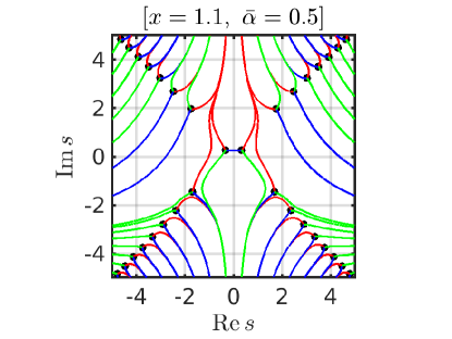
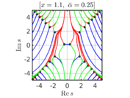
Figure 23: When the laser strength parameter $x$ reaches a certain lower bound for a given chirp ${\bar{\alpha}}$, then some equivalue lines that start at EPs from the lower half of the complex plane end up in the asymptotic limit ${\rm Im}\,s\to\infty$, i.e. in the integration half-plane.

I.4 Exponent in the asymptotic limit

Based on Eq. 560, the point $s_{BC,k}$ corresponds to $\xi=k$,

$${\rm Re}\,s_{BC,k}=\frac{(k+1/2)\pi}{{\rm Im}s}.$$ (568)

$Q(s)$ is defined in Eq. 212 as a reduced imaginary part of the quasienergy split. Note that the energy split $\tilde{\delta}(s)$, which is defined in Eq. 122, reads as

$$\tilde{\delta}(s)^{2}=e^{-[({\rm Re}s)^{2}-({\rm Im}s)^{2}]}e^{-2i{\rm Im}s{\rm Re}s}$$ (569)

$$\quad+\left(\frac{{\bar{\alpha}}}{2}({\rm Re}s+i{\rm Im}s)+\frac{i}{x}\right)^{2}$$ (570)

if the real and imaginary parts of $s$ are separated. Now, Eq. 570 is simplified for the case of the asymptotic limit, which is characterized by ${\rm Re}\,s\ll{\rm Im}\,s$ and ${\rm Im}\,s\gg 1$, from where

$$\tilde{\delta}(s)^{2}=$$ (571)

$$\quad e^{({\rm Im}s)^{2}}e^{-2i{\rm Im}s{\rm Re}s}-\left(\frac{{\bar{\alpha}}}{2}\right)^{2}({\rm Im}s)^{2}$$ (572)

$$\quad\approx e^{({\rm Im}s)^{2}}e^{-2i{\rm Im}s{\rm Re}s},$$ (573)

from where

$$\tilde{\delta}(s)\approx ze^{({\rm Im}s)^{2}/2}e^{-i{\rm Im}s{\rm Re}s}\ ,$$ (574)

where $z$ is an unknown sign. At this point it is useful to substitute for ${\rm Re}\,s$ using the contour parameter $\xi$ as defined in Eq. 560:

$$\tilde{\delta}(\xi)\approx-i\,ze^{({\rm Im}s)^{2}/2}e^{-i\pi\xi}\,.$$ (575)

$Q(s)$ defined by Eq. 212 is derived from Eq. 575 such that

$$Q(s)\approx-z\,x\,e^{({\rm Im}s)^{2}/2}\,\cos(\pi\xi)\,.$$ (576)

Now, we will substitute $Q(s)$ to Eq. 567, where we change the integration variable ${\rm Re}\,s^{\prime}$ for $\xi$ as defined in Eq. 560,

$$\gamma(s)=\gamma(s_{k+1})+\frac{\pi}{{\rm Im}s}\int\limits_{k}^{\xi}Q(\xi)\,d\xi,$$ (577)

such that

$$\gamma(s)=\gamma(s_{k+1})-z\cdot\frac{\pi\,xe^{({\rm Im}s)^{2}/2}}{{\rm Im}s}\sin(\pi\xi),$$ (578)

$$\quad k=floor(\xi),$$ (579)

where $\xi$ is defined in Eq. 560. Clearly, as $\xi$ acquires the limiting values on the integration contour, i.e. $k$ or $k+1$, then $\gamma(s)$ is finite given by $\gamma(s_{k+1})$. However, in between these two points, the absolute value of $\gamma(s)$ is infinite as ${\rm Im}\,s\to\infty$. If additionally the sign of $\gamma(s)$ is positive for $s_{k}<s<s_{k+1}$ then the integrand in Eq. 283 is infinitesimally small along the connecting contour in the asymptote, by which the use of the proposed integration contour would be justified. In the opposite case, the integrand would be infinite and the integration contour could not be used.

I.5 Sign alteration in the energy split when switching between equivalue lines

We can rewrite Eq. 579 such that

$$\gamma(s)=\gamma(s_{k+1})+[z\cdot(-)^{k+1}]\,\frac{\pi\,xe^{({\rm Im}s)^{2}/2}}{{\rm Im}s}|\sin(\pi\xi)|,$$ (580)

$$\quad k=floor(\xi).$$ (581)

Clearly, $\gamma(s)$ would be positive defined if

$$z=(-)^{k+1}.$$ (582)

As long as $z$ represents the sign of the energy split $\tilde{\delta}(s)$ in the asymptotic limit, see Eqs. 570–574, this indicates that the sign of the energy split would be changed when passing from one connecting line to another. This requirement makes sense if one recalls the fact that the sign is changed across the branchcuts.

Yet, only the sign alteration is not sufficient to assure that $z=(-)^{k+1}$, and not $z=(-)^{k}$, which would lead to a negative defined $\gamma(s)$. Namely, for $k=0$, $z<0$ for ${\rm Re}\,s>{\rm Re}s_{BC,0}$, and $z>0$ for ${\rm Re}s_{BC,0}>s>0$, while ${\rm Im}\,s\to\infty$. It follows from Eq. 574 that if this is satisfied then also ${\rm Im}\,\tilde{\delta}(s)<0$ (or equivalently $Q(s)<0$) as ${\rm Re}s\to+0$, while ${\rm Im}\,s\to\infty$. This happens if the same condition is satisfied also on the real axis:

$$Q(s)<0,\quad{\rm Re}\,s\to+0,\quad{\rm Im}\,s=0.$$ (583)

This condition is satisfied for bound to resonance transitions as follows from the definition in Eqs. 213. By this we proved that the contribution of the connecting lines between the branchcuts in the asymptotic limit $s\to i\infty$ is given by zero.

Appendix J Large pulse area limit for the branchcut contributions

Let us specify the laser parameters for which the limit defined by Eq. 304 is relevant by substituting for $\beta_{k}^{(1)}$ from Eq. 206:

$$\frac{x\Gamma\tau}{3\hbar}\left|{\bar{\alpha}}\left(\frac{{\bar{\alpha}}}{2}s_{k}+\frac{i}{x}\right)-2s_{k}\,e^{-s_{k}^{2}}\right|^{1/2}\to\infty,$$ (584)

which can be rewritten using the definition of the pulse area $\theta$ (Eq. 305) such that

$$\frac{\theta}{3\hbar}\cdot\sqrt{\frac{2}{\pi}}\cdot\left|{\bar{\alpha}}\left(\frac{{\bar{\alpha}}}{2}s_{k}+\frac{i}{x}\right)-2s_{k}\,e^{-s_{k}^{2}}\right|^{1/2}\to\infty.$$ (585)

The limit is exact for the very large pulse are $\theta\to\infty$, while it is at least approximately correct whenever the left hand side exceeds $\pi/2$, i.e. $\theta$ satisfies the condition

$$\theta>\frac{3\hbar\pi}{2}\sqrt{\frac{\pi}{2}}\cdot\left|{\bar{\alpha}}\left(\frac{{\bar{\alpha}}}{2}s_{k}+\frac{i}{x}\right)-2s_{k}\,e^{-s_{k}^{2}}\right|^{-1/2}.$$ (586)

Appendix K Continuity upon crossing the separatrix of odd and even layouts

We derived two different formulas for the survival probability applicable when encircling EP in the frequency–laser strength plane. The applicability of one or the other formula depends on the layout of the central pair of TPs in the complex adiabatic-time plane, which can be either “odd” or “even”. There is a division (separatrix) in the laser parameter plane, which designates the areas of the odd and even layouts, respectively, see Fig. 6. The separatrix is defined by the coalescence of the two TPs in the complex adiabatic-time plane. As the two TPs coalesce, a special second order TP arises for which the first order term in the Puiseux series is equal to zero.

The crossing of the separatrix is accompanied by the change of the formulas, which apply for the survival probability (of the initial bound state) $p_{1}$ such that

$$p_{1,odd}=\frac{\pi^{2}}{9}\exp\left[-\frac{2\,\theta}{\hbar\sqrt{2\pi}}\frac{\bar{\gamma}(s_{0i})}{x}\right],$$ (383 revisited)

$$p_{1,even}=$$

$$\frac{4\pi^{2}}{9}\exp\left[-\frac{2\,\theta}{\hbar\sqrt{2\pi}}\frac{\bar{\gamma}(s_{0i})}{x}\right]\cos^{2}\left[\frac{\theta}{\hbar\sqrt{2\pi}}\frac{\phi(s_{0})}{x}\right]\,.$$

Above we focused on the fact that these formulas predict the switch of the monotonic and oscillatory behavior and we showed physically achievable examples where this switch could be observable. Now we shall discuss a change of the survival probability $p_{1}$ upon crossing the separatrix, i.e. in the infinitesimal neighborhood of the crossing.

The function $\phi(s_{0})=0$ at the coalescence, which is shown in Fig. 17a. (This fact can be proved starting from the definition Eq. 215: At the coalescence, $s_{0}$ is purely imaginary, therefore the integration path is along the imaginary axis. At the same time, $\tilde{\delta}(s)$ is real-defined, which follows from the symmetric relation Eq. 47 and the fact that $\tilde{\delta}(s)$ is continuous in the infinitesimal neighborhood of the integration path. From here, the integral over $\tilde{\delta}(s)$ along this path is purely imaginary, thus $\phi(s_{0})=0$.) By substitution of $\phi(s_{0})$ we write the survival probability at the separatrix:

$$p_{1,odd}^{separatrix}=\frac{\pi^{2}}{9}\exp\left[-\frac{2\,\theta}{\hbar\sqrt{2\pi}}\frac{\bar{\gamma}(s_{0i})}{x}\right]\neq$$ (587)

$$\quad p_{1,even}^{separatrix}=\frac{4\pi^{2}}{9}\exp\left[-\frac{2\,\theta}{\hbar\sqrt{2\pi}}\frac{\bar{\gamma}(s_{0i})}{x}\right].$$ (588)

The left and right hand sides of the equation are different due to the different prefactor, as the rest of the functions is continuous at the crossing of the separatrix. Namely, the first-order perturbation theory predicts a topological phenomenon at the crossing of the separatrix in the laser pulse parameter plane for the asymptotic limit $\theta\to\infty$.

Keeping in mind that the formulas Eqs. 383 and 381 have been derived for the asymptotic limit $\theta\to\infty$, the convergence to this limit near the separatrix should be investigated. Let us use the asymptotic formulas Eqs. 383 and 381 as a basis for a parameter fitting for finite pulse area $\theta<\infty$. However for simplicity, instead of fitting the probability, we will fit the amplitude $v_{1}$

$$v_{1}^{odd}=a(\theta)\exp\left[-\frac{\theta}{\hbar\sqrt{2\pi}}\frac{\gamma(\theta)}{x}\right],$$ (589)

$$v_{1}^{even}=a(\theta)\exp\left[-\frac{\theta}{\hbar\sqrt{2\pi}}\frac{\gamma(\theta)}{x}\right]\cos\left[\frac{\theta}{\hbar\sqrt{2\pi}}\frac{\phi(\theta)}{x}\right]\,.$$ (590)

We will use the different fitting formulas on the different sides of the separatrix. It is expected that the fitted parameters $a(\theta)$, $\gamma(\theta)$, and $\phi(\theta)$ converge to the asymptotic limits as $\theta\to\infty$,

$$a^{odd}(\theta\to\infty)=\frac{\pi}{3}, a^{even}(\theta\to\infty)=\frac{2\pi}{3},$$ (592)

$$\gamma^{odd}(\theta\to\infty)=\gamma(s_{0i}), \gamma^{even}(\theta\to\infty)=\gamma(s_{0}),$$ (593)

$$\phi^{even}(\theta\to\infty)=\phi(s_{0}).$$ (594)

We use a numerical integration along the real axis to obtain $v_{1}$. As a matter of fact, numerical fitting procedures are not stable if the exponential parameter brings the value of $|v_{1}|$ below the computational precision. For these reasons we investigate a separatrix crossing which occurs not too far from $x=1$, where $\gamma(s_{0})$ and $\gamma(s_{0i})$ are almost zero, in particular, the separatrix crossing at ${\bar{\alpha}}=0.5$ and $x=1.0305$. We show the results of the fitting in Fig. 24.

Fig. 24a shows that the prefactor converges to different values for large pulse areas $\theta$ at the two opposite sides of the separatrix, which approves our previous conclusions based on analytical calculations. However, the convergence is slowed down in a close neigborhood of the separatrix. If we look at the exponent (Fig. 24b), we conclude that a change of the amplitude due to the exponent change when crossing the separatrix, compensates the jump in the prefactor several times at so large values of $\theta$. This explains the fact that the abrupt change of the prefactor is not demonstrated as an abrupt change of the survival probability $p_{1}$ when crossing the separatrix.

(a) (b)

Figure 24: Results of numerical fitting of the amplitude $v_{1}$ calculated using first order perturbation theory to the asymptotic formulas given by Eqs. LABEL:EQ15d2: (a) prefactor; (b) exponent. The laser parameter $x$ is changed from 1.0001 to 1.5, which ${\bar{\alpha}}=0.5$ for all calculations. The separatrix would be crossed at $x=1.0305$.

References

- [1] I. Rotter, A Non-Hermitian Hamilton Operator and the Physics of Open Quantum Systems, J. Phys. A-Math. Theor. 42 (2009) 153001. doi:{10.1088/1751-8113/42/15/153001}.
- [2] W. D. Heiss, The Physics of Exceptional Points, J. Phys. A-Math. Theor. 45 (2012) 444016. doi:{10.1088/1751-8113/45/44/444016}.
- [3] I. Rotter, J. P. Bird, A Review of Progress in the Physics of Open Quantum Systems: Theory and Experiment, Rep. Prog. Phys. 78 (2015) 114001. doi:{10.1088/0034-4885/78/11/114001}.
- [4] S. Klaiman, U. Guenther, N. Moiseyev, Visualization of Branch Points in PT-Symmetric Waveguides, Phys. Rev. Lett. 101 (2008) 080402. doi:{10.1103/PhysRevLett.101.080402}.
- [5] J. Doppler, A. A. Mailybaev, J. Bohm, U. Kuhl, A. Girschik, F. Libisch, T. J. Milburn, P. Rabl, N. Moiseyev, S. Rotter, Dynamically Encircling an Exceptional Point for Asymmetric Mode Switching, Nature. 537 (2016) 76. doi:{10.1038/nature18605}.
- [6] M.-A. Miri, A. Alu, Exceptional Points in Optics and Photonics, Science. 363 (2019) 7709.
- [7] M. Liertzer, L. Ge, A. D. Stone, H. E. Tuereci, S. Rotter, Pump-Induced Exceptional Points in Lasers, Phys. Rev. Lett. 108 (2012) 173901.
- [8] B. Peng, S. K. Ozdemir, S. Rotter, H. Yilmax, M. Liertzer, F. Monifi, C. M. Bender, F. Nori, L. Yang, Loss-Induced Suppression and Revival of Lasing, Science. 346 (2014) 328.
- [9] L. Feng, Z. J. Wong, R. M. Ma, Y. Wang, X. Zhang, Single-Mode Laser by Parity-Time Symmetry Breaking, Science. 346 (2014) 972. doi:{10.1126/science.1258479}.
- [10] S. K. Ozdemir, S. Rotter, F. Nori, L. Yang, Parity-Time Symmetry and Exceptional Points in Photonics, Nature. Mater. 18 (2019) 783.
- [11] P. R. Kapralova-Zdanska, N. Moiseyev, Helium in Chirped Laser Fields as a Time-Asymmetric Atomic Switch, J. Chem. Phys. 141 (2014) 014307. doi:{10.1063/1.4885136}.
- [12] B. Peng, W. Cao, C. Qu, J. Wen, L. Jiang, Y. Xiao, Anti-parity-time symmetry with flying atoms, Nat. Phys. 12 (2016) 1139.
- [13] L. Oberreiter, J. Burkhardt, J. Main, G. Wunner, Population transfer at exceptional points in the spectra of the hydrogen atom in parallel electric and magnetic fields, Phys. Rev. A 98 (2018) 013417.
- [14] J. Li, A. K. Harter, J. Liu, L. de Melo, Y. N. Joglekar, L. Luo, Observation of Parity-Time Symmetry Breaking Transitions in a Dissipative Floquet System of Ultracold Atoms, Nat. Commun. 10 (2019) 855.
- [15] H. Estrada, L. S. Cederbaum, W. Domcke, Vibronic Coupling of Short-lived Electronic States, J. Chem. Phys. 84 (1986) 152. doi:{10.1063/1.450165}.
- [16] R. Lefebvre, O. Atabek, M. Sindelka, N. Moiseyev, Resonance Coalescence in Molecular Photodissociation, Phys. Rev. Lett. 103 (2009) 123003. doi:{10.1103/PhysRevLett.103.123003}.
- [17] L. S. Cederbaum, Y.-C. Chiang, P. V. Demekhin, N. Moiseyev, Resonant Auger Decay of Molecules in Intense X-ray Laser Fields: Light-Induced Strong Nonadiabatic Effects, Phys. Rev. Lett. 106 (2011) 123001.
- [18] A. Leclerc, D. Viennot, G. Jolicard, R. Lefebvre, O. Atabek, Exotic States in the Strong-Field Control of H Dissociation Dynamics: From Exceptional Points to Zero-Width Resonances, J. Phys. B-At. Mol. Opt. Phys. 50 (2017) 234002.
- [19] Z. Benda, T.-C. Jagau, Locating Exceptional Points on Multidimensional Complex-Valued Potential Energy Surfaces, J. Phys. Chem. Lett. 9 (2018) 6978.
- [20] R. Uzdin, A. Mailybaev, N. Moiseyev, On the Observability and Asymmetry of Adiabatic State Flips Generated by Exceptional Points, J. Phys. A-Math. Theor. 44 (43) (2011) 435302. doi:{10.1088/1751-8113/44/43/435302}.
- [21] I. Gilary, A. A. Mailybaev, N. Moiseyev, Time-Asymmetric Quantum-State-Exchange Mechanism, Phys. Rev. A 88 (2013) 010102. doi:{10.1103/PhysRevA.88.010102}.
- [22] H. Xu, D. Mason, L. Y. Jiang, J. G. E. Harris, Topological Energy Transfer in an Optomechanical System with Exceptional Points, Nature. 537 (2016) 80. doi:{10.1038/nature18604}.
- [23] Q. Zhong, M. Khajavikhan, D. N. Christodoulides, R. El-Ganainy, Winding around non-Hermitian singularities, Nat. Commun. 9 (2018) 4808.
- [24] L. J. Fernandez-Alcazar, H. Li, F. Ellis, A. Alu, T. Kottos, Robust Scattered Fields from Adiabatically Driven Targets around Exceptional Points, Phys. Rev. Lett. 124 (2020) 133905.
- [25] J. Feilhauer, A. Schumer, J. Doppler, A. A. Mailybaev, J. Bohm, U. Kuhl, N. Moiseyev, S. Rotter, Encircling exceptional points as a non-Hermitian extension of rapid adiabatic passage, Phys. Rev. 102 (2020) 040201.
- [26] P. R. Kapralova, M. Sindelka, N. Moiseyev, Coalescence of Two Branch Points in Complex Time Marks the End of Rapid Adiabatic Passage and the Start of Rabi Oscillations, J. Phys. A-Math. Theor. (Submitted to the special issue on Claritons and the Asymptotics of Ideas: the Physics of Michael Berry.).
- [27] A. M. Dykhne, Adiabatic Perturbation of Discrete Spectrum States, Soviet Physics JETP 14 (1962) 941.
- [28] J. P. Davis, P. Pechukas, Nonadiabatic Transitions Induced by a Time-Dependent Hamiltonian in the Semiclassical/Adiabatic Limit: The Two-State Case, J. Chem. Phys. 64 (1976) 3129.
- [29] G. Dridi, S. Guerin, H. R. Jauslin, D. Viennot, G. Jolicard, Adiabatic Approximation for Quantum Dissipative Systems: Formulation, Topology, and Superadiabatic Tracking, Phys. Rev. A 82 (2010) 022109.
- [30] M. S. Child, Semiclassical Effects in Heavy-Particle Theory, Adv. in At. Mol. Phys. 14 (1979) 225.
- [31] S. L. McCall, E. L. Hahn, Self-induced transparency by pulsed coherent light, Phys. Rev. Lett. 18 (1967) 908.
- [32] S. L. McCall, E. L. Hahn, Self-induced transparency, Phys. Rev. 183 (1969) 183.
- [33] L. Allen, J. H. Eberly, Optical Resonance and Two-Level Atoms, Dover publications, inc., New York, 1987.
- [34] N. V. Vitanov, T. Halfmann, B. W. Shore, K. Bergmann, Laser-Induced Population Transfer by Adiabatic Passage Techniques, Annu. Rev. Phys. Chem. 52 (2001) 763. doi:{10.1146/annurev.physchem.52.1.763}.
- [35] R. Schilling, M. Vogelsberger, D. A. Garanin, Non-adiabatic Transitions for a Decaying Two-level System: Geometrical and Dynamical Contributions, J. Phys. A-Math. Gen. 39 (2006) 13727.
- [36] G. Dridi, S. Guerin, Adiabatic Passage for a Lossy Two-level Quantum System by a Complex Time Method, J. Phys. A-Math. Gen. 45 (2012) 185303.
- [37] N. Moiseyev, Non-hermitian quantum mechanics, Cambridge University Press, New York, 2011.
- [38] C. Zener, Non-adiabatic Crossing of Energy Levels, Proceedings. Of. The. Royal. Society. Of. London. Series. A-Mathematical. And. Physical. Sciences. 137 (1932) 696.
- [39] C. Wittig, The Landau-Zener Formula, J. Phys. Chem. B 109 (2005) 8428.
- [40] A. C. Vutha, A simple approach to the Landau-Zener formula, Eur. J. Phys. 31 (2010) 389. doi:{10.1088/0143-0807/31/2/016}.
- [41] S. N. Shevchenko, S. Ashhab, S. Nori, Landau-Zener-Stückelberg interferometry, Phys. Rep. 492 (2010) 1.
- [42] W. R. Thorson, J. B. Delos, S. A. Boorstein, Studies of the potential-curve crossing problem. I. Analysis of Stueckelberg’s method, Phys. Rev. A 4 (1971) 1052.
- [43] J. B. Delos, W. R. Thorson, Studies of the potential-curve crossing problem. II. General theory and a model for close crossings, Phys. Rev. A 6 (1972) 728.
- [44] T. Ota, K. Hitachi, K. Muraki, Landau-Zener-Stueckelberg interference in coherent charge oscillations of a one-electron double quantum dot, Sci. Rep. 8 (2018) 5491.
- [45] D. J. Tannor, Introduction to quantum mechanics – a time-dependent perspective, University Science Books, 2007.
- [46] N. V. Vitanov, K.-A. Suominen, Nonlinear Level-Crossing Models, Phys. Rev. A 59 (1999) 4580.
- [47] Y. Yan, B. Wu, Integral definition of transition time in the Landau-Zener model, Phys. Rev. A 81 (2010) 022126. doi:{10.1103/PhysRevA.81.022126}.
- [48] A. Pick, P. R. Kapralova-Zdanska, N. Moiseyev, Ab-initio Theory of Photoionization via Resonances, J. Chem. Phys. 150 (2019) 204111.