Tail contributions to gravitational conservative dynamics

Abstract

We compute tail contributions to the conservative dynamics of a generic self-gravitating system, for every multipole order, of either electric and magnetic parity. Such contributions arise when gravitational radiation is backscattered by the static curvature generated by the source itself and reabsorbed. Tail processes are relevant for the study of compact binary dynamics starting from the fourth post-Newtonian order. Within this context, we resolve a discrepancy recently arised at fifth post-Newtonian order between effective field theory and self-force results.

I Introduction

The recent detections of gravitational waves from coalescing binaries Abbott et al. (2019); Abbott et al. (2021a, b) by the large interferometers LIGO Aasi et al. (2015) and Virgo Acernese et al. (2015) have not only opened a new field in astronomy, but also revived theoretical studies of the general relativistic two-body problem.

Starting from the multipole expansion of a generic source, the focus of the present work is the contribution to the conservative dynamics of certain types of nonlinear effects, called tails, which are quadratic in Newton constant $G_{N}$ and arise when radiation is emitted, scattered onto the static potential generated by the same source, and finally absorbed. Tail effects have been first identified in emission processes, i.e., in the scattering of radiation off the source background curvature Blanchet and Damour (1988), and the leading contribution to the conservative dynamics of compact binaries has been first quantified in Foffa and Sturani (2013); see also Galley et al. (2016).

A common framework for dealing with two-body dynamics is the post-Newtonian (PN) approximation to General Relativity (GR) (see Blanchet (2014) for a review) that treats perturbatively the two-body problem and whose parameter of expansion is the binary relative velocity $v$, where the third Kepler’s law ensures $v^{2}\sim G_{N}M/r$, where $M$ is the binary system total mass and $r$ is the binary constituents’ distance. The PN approximation scheme is almost as old as GR itself; however, remarkably, it has been recast in recent times by Goldberger and Rothstein (2006) in a purely effective field theory (EFT) framework, dubbed nonrelativistic GR (NRGR) as it borrowed ideas from nonrelativistic QCD.

A technical detail of the NRGR framework, which is a common tool in field theory computations, is the distinction of the momenta of modes exchanged between sources, i.e., gravitational modes in NRGR, according to the region they belong to: hard or soft.

Potential modes sourced by conserved charges are of the former type, which are characterized by 4-momenta $k\sim(k_{0},{\bf k})$ with $|{\bf k}|\sim 1/r\gg k_{0}\sim v/r$, while radiative modes sourced by radiative multipoles have $|{\bf k}|\sim k_{0}$ and belong to the soft region. This separation is related to the distinction in a near and a far zone, commonly adopted in the traditional PN approach, where in the former binary constituents are resolved as individual objects and in the latter the binary system is described as a composite source endowed with multipoles. The complete dynamics is given by the sum of near and far zone processes Foffa and Sturani (2021), as it is well known from the particle physics application of the method of regions Manohar and Stewart (2007); Jantzen (2011).

The tail contributions presented in this work are linear in $M$ and quadratic in the nonconserved multipoles. The tail process involving electric quadrupole moments concur to determine the 4PN conservative dynamics of two-body system, which has now been obtained with three different methods independently by several groups Bini and Damour (2013); Damour et al. (2014); Bernard et al. (2016); Marchand et al. (2018); Foffa and Sturani (2019); Foffa et al. (2019); Blümlein et al. (2020) with mutually agreeing results.

Note that for obtaining the correct two-body dynamics, it is not enough to compute the tail effects in terms of multipoles, but also to derive the appropriate expression of the multipoles in terms of individual constituents, in a procedure that in the EFT language is called matching.

Since tail processes involve regularization of divergences, which we treated in dimensional regularization, to obtain the correct result it is crucial to have a multipole expression which is correct in generic $d$ dimensions. While this is straightforward for electric multipoles Blanchet et al. (2005), it involves some subtleties for magnetic ones, which are often expressed in terms of the Levi-Civita antisymmetric tensor $\epsilon_{ijk}$, which is not straightforwardly generalizable to $d\neq 3$. Besides computing in the present work for the first time tail terms for all multipoles, we solve the puzzle arised by the apparent discrepancy between the conservative dynamics NRGR result at 5PN, obtained in Foffa and Sturani (2020) for the far zone and in Blümlein et al. (2021a) for the potential modes, and the derivation of the two-body scattering angle from the “Tutti Frutti” approach Bini et al. (2019, 2020), as presented in Bini et al. (2021), at next-to-leading order in symmetric mass ratio $\nu=m_{1}m_{2}/M^{2}$, having denoted by $m_{1,2}$ the masses of the binary constituents. We show here that agreement is indeed found between the two approaches when magnetic multipoles are properly defined in generic $d$ dimensions, as in Henry et al. (2021).

The outline of the paper is as follows: in Sec. II we perform the computation of the tail process for generic multipoles, completing it in Sec. III with the necessary matching procedure, which enables one to write the multipoles in terms of the binary constituents’ variables. In Sec. IV we explain the origin of the discrepancy found in Blümlein et al. (2021a); Bini et al. (2021) and show its solution, and Sec. V contains the conclusions that can be drawn from our results.

II Far zone calculations

We adopt the following parametrization for the multipolar expansion of the gravitational coupling of a composite system:

$${\cal S}_{\text{mult}} =\int{\rm d}t\left[\frac{1}{2}Eh_{00}-\frac{1}{2}J^{b|a}h_{0b,a}-\sum_{r\geq 0}\left(c^{(I)}_{r}I^{ijR}\partial_{R}R_{0i0j}+\frac{c^{(J)}_{r}}{2}J^{b|iRa}\partial_{R}R_{0iab}\right)\right]\,,$$ (1)

with Thorne (1980); Ross (2012)

$$c_{r}^{(I)}=\displaystyle\frac{1}{\left(r+2\right)!}\,,\quad c_{r}^{(J)}=\displaystyle\frac{2\left(r+2\right)}{\left(r+3\right)!}\,,$$ (2)

where $E$ denotes the energy of the system and $h_{\mu\nu}$ indicates the metric deviation from Minkowski, i.e., $g_{\mu\nu}=\eta_{\mu\nu}+h_{\mu\nu}$. We denote the generic electric traceless multipoles by $I^{ijR}\equiv I^{iji_{1}\dots i_{r}}$, using the collective index $R$, and the magnetic traceless multipoles by $J^{b|iRa}\equiv J^{b|ii_{1}\dots i_{r}a}$ (antisymmetric under $a\leftrightarrow b$), using the $d$-dimensional generalization of the magnetic moments recently proposed in Henry et al. (2021), which are described in Appendix B. The tail process we are interested in is described by the diagram in Fig. 1. It represents the leading far zone contribution to the conservative dynamics, i.e., the leading contribution from diagrams involving radiative gravitational fields.

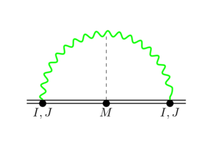
Figure 1: Self-energy diagram for a generic radiative multipole source of electric and magnetic type. The green wavy (dashed straight) line represents the radiative (potential) gravitational field, while the black double line stands for the composite source described by the multipolar action in Eq. (1).

The solid double line represents the nonpropagating source of Eq. (1), characterized by conserved energy and angular momentum, and time-dependent electric and magnetic multipoles; wavy lines represent radiative mode Green’s function and the dashed line stands for the potential mode Green’s function, meeting at the triple bulk vertex where the scattering of radiation off the potential happens. Using standard Feynman rules for the worldline and bulk vertices involved (see, e.g., Foffa and Sturani (2020)) and adopting the notation $p_{R}\equiv p_{i_{1}\dots i_{r}}$ and $\int_{{\bf p}\,{\bf q}}\equiv\int\frac{{\rm d}^{d}p}{(2\pi)^{d}}\frac{{\rm d}^{d}q}{(2\pi)^{d}}$, one has

$$\displaystyle{\cal S}^{(e,r)}_{tail} = \displaystyle-\frac{[c_{r}^{(I)}]^{2}E}{4\Lambda^{4}}\int\frac{{\rm d}p_{0}}{2\pi}\int_{{\bf p},{\bf q}}\frac{p_{R}q_{R^{\prime}}I^{ijR}(p_{0})I^{klR^{\prime}}(-p_{0})}{\left({\bf p}^{2}-p_{0}^{2}\right)\left({\bf q}^{2}-p_{0}^{2}\right)\left({\bf q}-{\bf p}\right)^{2}}$$ (3)

$$\times \left\{-\frac{1}{4}p_{0}^{6}\delta_{ik}\delta_{jl}-p_{0}^{4}\delta_{ik}p_{j}\left(q-p\right)_{l}-\frac{p_{0}^{2}}{c_{d}}p_{i}p_{j}\left[\left(q-p\right)_{k}\left(q-p\right)_{l}+\frac{1}{2}q_{k}q_{l}\right]\right.$$

$$\quad\left.+\frac{p_{0}^{2}}{2}p_{i}q_{k}\left[{\bf p}\cdot{\bf q}\delta_{jl}+p_{j}q_{l}-p_{l}q_{j}\right]\right\}$$

$$= -\frac{E}{(32\pi\Lambda^{2})^{2}}\frac{(d-2)\Gamma\left(d-3\right)\Gamma\left(2-\frac{d}{2}\right)\Gamma\left(-\frac{d}{2}-1-r\right)}{2^{r}(4\pi)^{d-2}(d-1)(r+1)^{2}(r+2)^{2}\Gamma\left(d+r\right)}\zeta^{(e)}_{d,r}$$

$$\displaystyle\quad\times\int\frac{{\rm d}p_{0}}{2\pi}(-p_{0}^{2})^{d+r}I^{ijR}(p_{0})I^{ijR}(-p_{0})$$

with

$$\zeta^{(e)}_{d,r} \equiv d^{4}+2(r-2)d^{3}+\left(3r^{3}-3r+5\right)d^{2}+\left(r-2\right)\left(2r^{2}+r+1\right)d+\left(r+1\right)^{2}\left(r^{2}+2r+12\right)$$ (4)

$$= (r+1)(r+2)(r+3)(r+4)+(r+4)(2r^{2}+7r+7)\varepsilon+{\cal O}\left(\varepsilon^{2}\right)\,,\quad\varepsilon\equiv d-3\,,$$

which can be obtained using the master integral reported in Appendix A; see also Almeida et al. (2021). It has been necessary to introduce a $d$-dimensional Newton constant in the form $G_{d}=\mu^{d-3}\left(32\pi\Lambda^{2}\right)^{-1}$, with $\Lambda\equiv(32\pi G_{N})^{-1/2}$, where $\mu$ is an arbitrary, inverse length scale needed to adjust dimensions.

Expansion around $d\sim 3$ gives

$$\displaystyle{\cal S}^{(e,r)}_{tail} \simeq -G_{N}^{2}E\frac{2^{r+2}(r+3)(r+4)}{(r+1)(r+2)(2r+5)!}\int\frac{{\rm d}p_{0}}{2\pi}(p_{0}^{2})^{r+3}I^{ijR}(p_{0})I^{ijR}(-p_{0})\left[\frac{1}{\tilde{\varepsilon}}-\gamma^{(e)}_{r}\right]$$ (5)

with

$$\frac{1}{\tilde{\varepsilon}}\equiv\frac{1}{\varepsilon}-{\tt i}\pi+\log\left(\frac{p_{0}^{2}{\rm e}^{\gamma}}{\pi\mu^{2}}\right)$$ (6)

and

$$\begin{array}[]{rcl}\displaystyle\gamma^{(e)}_{r}&\equiv&\displaystyle\frac{1}{2}\left(H_{r+\frac{5}{2}}-H_{\frac{1}{2}}+2H_{r}+1\right)+\frac{2}{(r+2)(r+3)}\\ &=&\displaystyle\left\{\frac{41}{30},\frac{82}{35},\frac{1819}{630},\frac{11359}{3465},\frac{646141}{180180},\dots\right\}\,,\end{array}$$ (9)

where $H_{r}$ is the $r$th harmonic number defined by $H_{r}\equiv\sum_{i=0}^{r}1/i$. The structure contained in Eq. (6), whose precoefficient in the tail action is the opposite of the one multiplying the multipole contribution to the flux Thorne (1980) (see below), is universal for all multipoles and has been analyzed in Foffa and Sturani (2020). It has been obtained using Feyman Green’s functions, which give for the real part the same result as it would be obtained by adopting causal boundary conditions, that is, an UV pole, to be matched by an IR pole coming from the near zone, and the nonlocal (in time) contribution discovered in Blanchet and Damour (1988). The imaginary part, which is of no interest for the present work, is related via the optical theorem to the energy flux in tail process; see Foffa and Sturani (2021) for a thorough discussion on the appropriate choice of the boundary conditions.

Coming to the first new result of this work, that is, the $\gamma^{(e)}_{r}$ term displayed Eq. (9), we notice that it is rational because the irrational terms contained in $H_{r+\frac{5}{2}}$ and $H_{\frac{1}{2}}$ cancel in the difference $\displaystyle H_{r+\frac{5}{2}}-H_{\frac{1}{2}}=2\sum_{i=1}^{r+2}\frac{1}{2i+1}$. The first two values $\gamma^{(e)}_{0}$ and $\gamma^{(e)}_{1}$ correspond to the electric quadrupole and octupole finite and local-in-time contributions computed, respectively, in Foffa and Sturani (2013) and Foffa and Sturani (2020).

An analogous computation for the magnetic moments gives

$$\displaystyle{\cal S}^{(m,r)}_{\textrm{tail}} = \displaystyle\frac{[c_{r}^{(J)}]^{2}E}{32\Lambda^{4}}\int\frac{{\rm d}p_{0}}{2\pi}J_{l|jRk}(p_{0})J_{n|aR^{\prime}m}(-p_{0})\int_{{\bf p},{\bf q}}\frac{p_{R}q_{R^{\prime}}}{\left({\bf p}^{2}-p_{0}^{2}\right)\left({\bf q}^{2}-p_{0}^{2}\right)\left({\bf q}-{\bf p}\right)^{2}}$$

$$\times\displaystyle\bigg{\{}p_{0}^{4}p_{l}q_{n}\left(\delta_{ja}\delta_{km}+\delta_{jm}\delta_{ka}\right)+2p_{0}^{2}p_{l}q_{m}p_{j}\left[\delta_{ka}p_{n}+\delta_{kn}(p-q)_{a}\right]$$

$$\displaystyle\quad-q_{a}q_{m}p_{j}p_{k}\left({\bf p}\cdot{\bf q}\delta_{ln}-q_{l}p_{n}\right)\bigg{\}}$$

$$= -\frac{E}{(32\pi\Lambda^{2})^{2}}\frac{\Gamma\left(d-3\right)\Gamma\left(2-\frac{d}{2}\right)\Gamma\left(-\frac{d}{2}-1-r\right)}{2^{r-1}(4\pi)^{d-2}(r+1)(r+3)^{2}\Gamma\left(d+r+1\right)}\left[d^{2}+d(r-2)+r^{2}+2r+3\right]$$

$$\quad\times\left(d+r+1\right)\int\frac{{\rm d}p_{0}}{2\pi}(-p_{0}^{2})^{d+r}J_{l|jRk}(p_{0})J_{n|aRk}(-p_{0})\left[\delta_{ja}\delta_{ln}+(r+1)\delta_{jn}\delta_{la}\right]\,.$$

Expansion around $d\sim 3$ gives

$$\begin{array}[]{rcl}\displaystyle{\cal S}^{(m,r)}_{tail}&\simeq&\displaystyle-G_{N}^{2}E\frac{2^{r+4}(r+2)(r+4)}{(r+1)(r+3)^{2}(2r+5)!}\\ &&\displaystyle\quad\times\int\frac{{\rm d}p_{0}}{2\pi}(p_{0}^{2})^{r+3}J_{l|jRk}(p_{0})J_{n|aRk}(-p_{0})\left[\delta_{ja}\delta_{ln}+(r+1)\delta_{jn}\delta_{la}\right]\left[\frac{1}{\tilde{\varepsilon}}-\gamma^{(m)}_{r}\right]\end{array}$$ (13)

with

$$\begin{array}[]{rcl}\displaystyle\gamma^{(m)}_{r}&\equiv&\displaystyle\frac{1}{2}\left(H_{r+\frac{5}{2}}-H_{\frac{1}{2}}+2H_{r+3}+2\right)-\frac{2r^{2}+13r+22}{(r+2)(r+3)(r+4)}\\ &=&\displaystyle\left\{\frac{49}{20},\frac{22}{7},\frac{4541}{1260},\frac{1565}{396},\frac{1525229}{360360}\dots\right\}\,.\end{array}$$ (16)

Also in the magnetic case, the numerical coefficient in front of the $\varepsilon$ pole reproduces, for $d=3$, the magnetic emission coefficients which, however, in the commonly used formula for the energy flux $F$ appears as (see Appendix A)

$$F=G_{N}\sum_{r\geq 0}\bigg{[}f_{I}(r)\Big{\langle}\left(\frac{{\rm d}^{r+3}}{{\rm d}t^{r+3}}I_{ijR}\right)^{2}\Big{\rangle}+f_{J}(r)\Big{\langle}\left(\frac{{\rm d}^{r+3}}{{\rm d}t^{r+3}}J_{ijR}\right)^{2}\Big{\rangle}\bigg{]}\,,$$ (17)

i.e., they multiply the square of the magnetic multipole $J_{ijR}$, which is dual to the $J_{l|jRk}$ used above Henry et al. (2021):

$$J_{l|jRk}\stackrel{{\scriptstyle d=3}}{{=}}\epsilon^{ilk}J_{ijR}\,.$$ (18)

When substituting in the result of Eq. (13) the relation (18) one finds $J_{l|jRk}J_{n|aRk}\left[\delta_{ja}\delta_{ln}+(r+1)\delta_{jn}\delta_{la}\right]\stackrel{{\scriptstyle d=3}}{{=}}(r+3)J_{ijR}^{2}$ which reproduces the magnetic emission coefficients first derived by Thorne (1980). As for the finite part proportional to $\gamma^{(m)}_{r}$ in Eq. (13), care is needed to match to the binary constituents’ variables, which will be done in Sec. III, and to extract the correct $d\to 3$ limit, which will be done in Sec. IV.

III Matching

Following standard GR textbook derivation (see Appendix B for details) the linear gravitational coupling of an extended source can be written in terms of the nonconserved source multipoles. Working in the transverse-traceless (TT) gauge for simplicity, and focusing for the moment on the electric multipoles, one can write

$${\cal S}_{mult-e}=\frac{1}{2}\int{\rm d}t\left(\frac{1}{2}\ddot{I}_{ij}h_{ij}+\frac{1}{6}\ddot{I}^{ijk}h_{ij,k}+\ldots\right)\,,$$ (19)

where at lowest order

$$I^{ij}=\int_{V}T^{00}x^{i}x^{j}\,,$$ (20)

$$I^{ijk}=\int_{V}T^{00}x^{i}x^{j}x^{k}\,,$$ (21)

where $T^{\mu\nu}$ is the energy-momentum tensor of a generic source and we adopted the notation $\int_{V}\equiv\int{\rm d}^{d}x$. For the magnetic ones, one needs some extra care, in view of the $d$-dimensional generalization which is needed for Eq. (13). Taylor expanding the standard, generic gravitational coupling $\frac{1}{2}T^{\mu\nu}h_{\mu\nu}$ at next-to-leading order for the spatial components $T^{ij}$, one obtains (see Appendix B for details)

$$\begin{array}[]{rcl}\displaystyle\frac{1}{2}\int_{V}T^{ij}x^{k}&=&\displaystyle\frac{1}{6}\int_{V}\left(T^{ij}x^{k}+T^{ki}x^{j}+T^{jk}x^{i}\right)+\frac{1}{6}\int_{V}\left(2T^{ij}x^{k}-T^{ik}x^{j}-T^{jk}x^{i}\right)\,,\\ &=&\displaystyle\frac{1}{12}\frac{{\rm d}^{2}}{{\rm d}t^{2}}\left(\int_{V}T^{00}x^{i}x^{j}x^{k}\right)+\frac{1}{6}\frac{\rm d}{{\rm d}t}\left[\int_{V}\left(T^{0i}x^{k}x^{j}+T^{0j}x^{k}x^{i}-2T^{0k}x^{i}x^{j}\right)\right]\,.\end{array}$$ (24)

The first term in the second line of Eq. (24) is the electric octupole contribution, whereas the second term is the magnetic quadrupole one, which is often written in terms of

$$J^{ij} \stackrel{{\scriptstyle d=3}}{{\equiv}} \displaystyle\frac{1}{2}\int_{V}x^{m}T^{0n}\left(x^{i}\epsilon^{jmn}+x^{j}\epsilon^{imn}\right)\,,$$ (25)

which is symmetric in $i,j$ and traceless. Using the identity

$$\begin{array}[]{l}\displaystyle\left(T^{0i}x^{k}-T^{0k}x^{i}\right)x^{j}h_{ij,k}=T^{0m}x^{n}x^{j}\left(\delta^{l}_{m}\delta^{k}_{n}-\delta^{k}_{m}\delta^{l}_{n}\right)h_{lj,k}\\ \displaystyle\stackrel{{\scriptstyle d=3}}{{=}}-\epsilon_{imn}x^{m}T^{0n}x^{j}\epsilon^{ilk}\times\frac{1}{2}\left(h_{lj,k}-h_{kj,l}\right)\,,\end{array}$$

and the definition of the magnetic part of the Riemann tensor ${\cal B}_{ij}\stackrel{{\scriptstyle d=3}}{{\equiv}}\frac{1}{2}\epsilon_{imn}R_{0jmn}$, one finds the magnetic quadrupole multipole term

$${\cal S}_{mult-m}\stackrel{{\scriptstyle d=3}}{{=}}\frac{2}{3}\int dt\left(J^{ij}{\cal B}_{ij}+\ldots\right)\,.$$ (26)

To avoid the use of the Levi-Civita tensor $\epsilon_{ijk}$ which may not be straightforwardly generalizable to $d\neq 3$, it is useful to write the magnetic quadrupole term coupled to gravity as

$$\begin{array}[]{l}\displaystyle\left.\frac{1}{2}\left(\int_{V}T^{ij}x^{k}\right)h_{ij,k}\right|_{magnetic}=-\frac{1}{3}\left[\int_{V}x^{j}\left(T^{0i}x^{k}-T^{0k}x^{i}\right)\right]\dot{h}_{ij,k}\\ \displaystyle=\frac{1}{3}\left[\int_{V}x^{j}\left(T^{0i}x^{k}-T^{0k}x^{i}\right)\right]\times\frac{1}{2}\left(\dot{h}_{kj,i}-\dot{h}_{ij,k}\right)=-\frac{1}{3}J^{k|ji}R_{0jik}\,,\end{array}$$ (29)

where an integration by parts has been used and in the last passage the linearized expression for the Riemann in the TT gauge, $R_{0ijk}\sim\frac{1}{2}\left(\dot{h}_{ij,k}-\dot{h}_{ik,j}\right)$, has been inserted. Note that since $R_{0ijk}$ has vanishing traces for pure radiation, one is led to define the magnetic quadrupole as

$$J^{i|jk}\equiv\int_{V}x^{j}\left(T^{0k}x^{i}-T^{0i}x^{k}\right)-\frac{\delta^{kj}}{d-1}\left(x_{m}T^{0m}x^{i}-{\bf x}^{2}T^{0i}\right)+\frac{\delta^{ij}}{d-1}\left(x_{m}T^{0m}x^{k}-{\bf x}^{2}T^{0k}\right)\,,$$ (30)

which is antisymmetric in the index pair $i,k$, traceless, and, in $d=3$, it is the dual of $J^{ij}$ in (25), as per Eq. (18) with no “$R$” indices.

At the leading order in source internal velocity and self-gravity, it is actually trivial to match the multipoles to binary constituents’ parameters, to obtain

$$\begin{array}[]{rcl}\displaystyle I^{ij}&=&\displaystyle\left(\sum_{a}m_{a}x_{a}^{i}x_{a}^{j}\right)_{TF}\,,\\ \displaystyle I^{ijk}&=&\displaystyle\left(\sum_{a}m_{a}x_{a}^{i}x_{a}^{j}x_{a}^{k}\right)_{TF}\,,\\ \displaystyle J^{i|jk}&=&\displaystyle\left(\sum_{a}m_{a}(x_{a}^{i}v_{a}^{k}-v_{a}^{i}x_{a}^{k})x_{a}^{j}\right)_{TF}\,,\end{array}$$ (31)

where “$TF$” stands for trace-free. Evaluating them in the center of mass frame, one obtains

$${\cal S}_{\textrm{mult}}\supset-\int{\rm d}t\left[\frac{1}{2}I^{ij}R_{0i0j}+\frac{1}{6}I^{ijk}R_{0i0j,k}+\frac{1}{3}J^{b|ia}R_{0iab}\right]\,,$$ (32)

where in the TT gauge $R_{0i0j}\simeq-\frac{1}{2}\ddot{h}_{ij}$ and, at leading order,

$$\begin{array}[]{rcl}I^{ij}&=&\displaystyle\nu M\left(x^{i}x^{j}\right)_{TF}\,,\\ I^{ijk}&=&\displaystyle\nu\Delta m\left(x^{i}x^{j}x^{k}\right)_{TF}\,,\\ J^{b|ia}&=&\displaystyle\nu\Delta m\left[x^{i}x^{b}v^{a}-\frac{{\bf x}^{2}}{d-1}\delta^{ib}v^{a}-\frac{{\bf x}\cdot{\bf v}}{d-1}\delta^{ia}x^{b}-\left(a\leftrightarrow b\right)\right]\,,\end{array}$$ (36)

where $\Delta m\equiv M\sqrt{1-4\nu}$ and $\nu\equiv m_{1}m_{2}/M^{2}$ is the symmetric mass ratio. This expression for the magnetic quadrupole is valid for any $d$; hence, its expression can be safely plugged into Eq. (13) to obtain the correct conservative action.

IV Explicit form of 5PN tail terms and comparison with previous results

We can now plug Eq. (36) into the expressions for ${\cal S}^{(e,1)}_{tail}$ and ${\cal S}^{(m,0)}_{tail}$ reported in Sec. II and obtain the tail terms as functions of the binary variables. We focus on these two contributions as they are the ones whose lowest order contribution is at 5PN, which is where Blümlein et al. (2021a); Bini et al. (2021) have shown disagreement with the extreme-mass ratio result. After reducing higher order derivatives by means of the Newtonian equations of motion, and neglecting logarithms and the imaginary part, which are anyways completely determined by the dimensional pole, the result takes the following form:

$$\displaystyle{\cal S}^{(e,1)}_{tail} \simeq \displaystyle-\frac{G_{N}^{4}M^{3}}{189}\nu^{2}\Delta m^{2}\int\frac{{\rm d}t}{r^{4}}\bigg{\{}\frac{1}{\varepsilon}\left[\frac{6042}{5}v^{4}-2364v^{2}v_{r}^{2}+1170v_{r}^{4}\right.$$

$$\displaystyle\qquad\left.+\frac{G_{N}M}{r}\left(\frac{1872}{5}v^{2}-432v_{r}^{2}\right)+\frac{288}{5}\frac{G_{N}^{2}M^{2}}{r^{2}}\right]+\frac{157887}{175}v^{4}-\frac{68442}{35}v^{2}v_{r}^{2}$$

$$\displaystyle\qquad+\frac{7167}{7}v_{r}^{4}+\frac{G_{N}M}{r}\left(\frac{124452}{175}v^{2}-\frac{26316}{35}v_{r}^{2}\right)+\frac{34848}{175}\frac{G_{N}^{2}M^{2}}{r^{2}}\bigg{\}}\,,$$

$$\displaystyle{\cal S}^{(m,0)}_{tail} \simeq \displaystyle-\frac{16G_{N}^{4}M^{3}}{45}\nu^{2}\Delta m^{2}\int\frac{{\rm d}t}{r^{4}}\left\{\frac{1}{\varepsilon}\left[\frac{1}{2}v^{4}+v^{2}v_{r}^{2}-\frac{3}{2}v_{r}^{4}\right]+\frac{21}{40}v^{4}+\frac{61}{20}v^{2}v_{r}^{2}-\frac{143}{40}v_{r}^{4}\right\}\,,$$ (38)

with $v_{r}\equiv\frac{{\bf r}\cdot{\bf v}}{r}$. Both results are in agreement with the self-force determination of the scattering angle, as it has been checked in Blümlein et al. (2021a) and then confirmed in Bini et al. (2021). However, the magnetic quadrupole result in Eq. (38) is different from what would be obtained by substituting Eq. (25) into the analog result for Eq. (13) obtained in Foffa and Sturani (2020), which is expressed in terms of the three-dimensional form of the magnetic quadrupole $J^{ij}$, instead of its dual $J^{k|ji}$, whose introduction is subsequent to Foffa and Sturani (2020).

To understand the origin of the discrepancy, let us replace $J^{a|jb}$ with its dual expression (18) inside Eq. (13) for $r=0$, to obtain its dual version

$${\cal S}^{(m,0)}_{tail-dual} \equiv \int{\rm d}t\left(\dddot{J_{ij}}\right)\epsilon_{ilk}T^{jkbc}\delta^{ld}\epsilon_{adc}\left(\dddot{J_{ab}}\right)\,,$$ (39)

where

$$T^{jkbc}\simeq-\frac{16G_{N}^{2}E}{135}\left(\delta^{jb}\delta^{kc}+\delta^{jc}\delta^{kb}\right)\times\left(\frac{1}{\tilde{\varepsilon}}-\frac{49}{20}\right)$$

which is the result reported in Bini et al. (2021), and which, after using the three-dimensional relation $\epsilon_{ilk}\epsilon_{adc}\delta^{ld}=\delta_{ia}\delta_{kc}-\delta_{ic}\delta_{ka}$, gives

$${\cal S}^{(m,0)}_{tail-dual} = \displaystyle-\frac{16G_{N}^{2}E}{135}\int{\rm d}t\left(\dddot{J_{ij}}\right)\left(d\delta_{ai}\delta_{bj}-\delta_{ab}\delta_{ij}\right)\left(\dddot{J_{ab}}\right)\times\left(\frac{1}{\tilde{\varepsilon}}-\frac{49}{20}\right)$$ (40)

$$\simeq -\frac{16G_{N}^{2}E}{45}\int{\rm d}t\left(\frac{1}{\tilde{\varepsilon}}-\frac{127}{60}\right)\left(\dddot{J_{ij}}\right)^{2}\,,$$

which is the result computed in Foffa and Sturani (2020).

We note, however, that the identification (18) is valid only for $d=3$; hence, one is allowed to use it only as long as the final result is finite. The conservative Lagrangian is indeed finite, but the two separate contributions coming from the far and the near zone, computed, respectively, in Foffa and Sturani (2020) and in Blümlein et al. (2021a), have $\varepsilon$ poles in dimensional regularization. In principle, it is possible to use the far zone expression in terms of the $J_{ij}$ variables if a similar manipulation is also performed in the near zone diagrams corresponding to the magnetic quadrupole tail, along the lines discussed in Appendix B of Foffa et al. (2019), which treats in detail the 4PN case. This is, however, a cumbersome procedure and a much simpler alternative, as done in the present work, is to completely avoid the use of $J_{ij}$, and stick to the $d$-dimensional form for the magnetic multipoles in the far zone which leads to Eq. (13), and not use the result in Eq. (40).

This explains the discrepancy observed in Blümlein et al. (2021a), where it is observed that Eq. (40) is incompatible with the result obtained via scattering angle/extreme mass ratio limit computation Bini et al. (2019, 2020), unless the coefficient $-127/60$ is offset by $-1/6$. In Bini et al. (2021), building on Tutti Frutti approach results Bini et al. (2019, 2020), a different offset is invoked because a different expression for $J_{ij}$ with respect to Blümlein et al. (2021a) [namely, the inverse of Eq. (18), instead of Eq. (25)] is assumed. However, this is just a formal difference, and both Blümlein et al. (2021a) and Bini et al. (2021) agree on the only expression compatible with the scattering angle/extreme mass ratio determination is the one reported in Eq. (38) in the Lagrangian formalism.

V Conclusion

We have formally computed all the tail contributions to the conservative dynamics of a generic binary system. Such computation makes use of the recently introduced $d$-dimensional generalization of the magnetic gravitational multipoles and, when applied to the specific case of compact binaries, allowed us to reconcile the effective field theory result with the scattering angle one at next-to-leading order in the symmetric mass ratio $\nu$ at 5PN order. Note that finite size effects for spinless black holes vanish in the static limit Binnington and Poisson (2009); Damour and Nagar (2009); Kol and Smolkin (2012); hence, they affect the dynamics at higher than 5PN order, which is the lowest order admissible by the effacement principle Damour (1982). The expression of the scattering angle is still incomplete at next-to-next-to-leading order in $\nu$, but even the present partial knowledge is enough to show Bini et al. (2021) that such a sector is incompatible with the effective field theory near+far zone result obtained so far, which involves, among other terms on the far zone side, the nonlinear memory process due to emission, scattering, and absorption of radiation Blanchet and Damour (1992). We leave the investigation of this remaining mismatch to future work.

Appendix A Useful formulas

To perform the computations in Sec. II one needs the master integral

$$\int_{{\bf p}{\bf q}}\frac{1}{{\cal D}_{a}} = \left(-p_{0}^{2}\right)^{d-2-a}I_{a}\,,$$ (41)

where we adopted the notation ${\cal D}_{a}\equiv\left({\bf p}^{2}-p_{0}^{2}\right)\left({\bf q}^{2}-p_{0}^{2}\right)\left({\bf q}^{2}-{\bf p}^{2}\right)^{a}$, and

$$I_{a}\equiv\frac{1}{\left(4\pi\right)^{d}}\frac{\Gamma\left(a+2-d\right)\Gamma\left(a+1-d/2\right)^{2}\Gamma\left(d/2-a\right)}{\Gamma\left(2a+2-d\right)\Gamma\left(d/2\right)}\,.$$ (42)

Note that we have been cavalier about the Green’s function boundary conditions, i.e., about the displacement off the real axis of the Green’s functions poles. We are allowed to do so because, as derived in Foffa and Sturani (2021), casual or time symmetric boundary conditions give the same result for the real part of diagrams with up to two Green’s functions for radiative modes, and the imaginary part of the diagrams do not contribute to the conservative dynamics we are computing here.

In addition one needs the tensor integral

$$\begin{array}[]{l}\displaystyle\int_{\bf q}\frac{q_{i_{1}}\dots q_{i_{n}}}{\left[\left({\bf k}-{\bf q}\right)^{2}\right]^{a}\left[{\bf q}^{2}-(\omega+i\tt{a})^{2}\right]^{b}}=\sum_{m=0}^{[n/2]}S_{a,b}[n,m]\{[\delta]^{m}[k]^{n-2m}\}_{i_{1}\cdots i_{n}}\,,\\ \displaystyle S_{a,b}[n,m]\equiv\frac{\left[-\left(\omega+i\tt{a}\right)^{2}\right]^{d/2-a-b+m}}{2^{m}\left(4\pi\right)^{d/2}}\frac{\Gamma(a+b-d/2-m)\Gamma(a+n-2m)\Gamma(d+2m-2a-b)}{\Gamma(a)\Gamma(b)\Gamma(d+n-a-b)}\,.\end{array}$$ (45)

The explicit expression of the Thorne coefficients appearing in Eq. (17) is

$$\begin{array}[]{rcl}\displaystyle f_{I}(r)&=&\displaystyle\frac{(r+3)(r+4)}{(r+1)(r+2)(r+2)!(2r+5)!!}\,,\\ \displaystyle f_{J}(r)&=&\displaystyle\frac{4(r+2)(r+4)}{(r+1)(r+3)!(2r+5)!!}\,.\end{array}$$ (48)

Appendix B Detailed matching procedure for the magnetic moments

We give here an alternative, detailed procedure for the matching of the magnetic moments for the specific case of a binary system, whose coupling to radiation is described by the diagrams in Fig. 2.

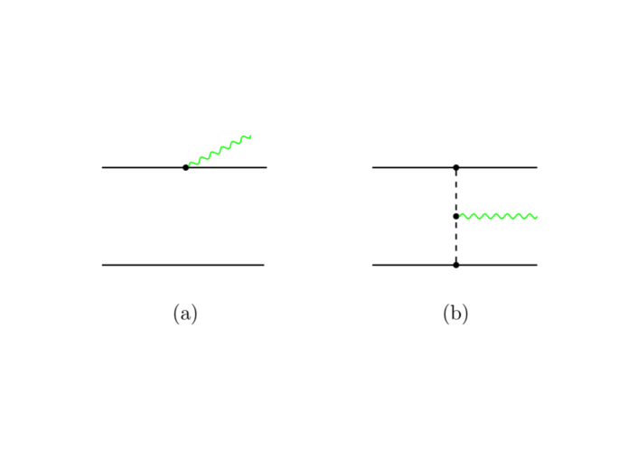
Figure 2: Diagrams representing the leading order coupling of a binary system to radiative gravitational modes. While diagram (a) yields the first term in Eq. (B1), diagram (b) accounts for the rest of the expression.

We are particularly interested in the coupling of gravitational radiation with the first moment of $T^{ij}$, which gives rise to the mass octupole and to the current quadrupole couplings as per Eq. (24). By expanding up to the first order in the external gravitational mode momentum ${\bf q}$, and working in the TT gauge, the sum of the two diagrams gives $1/2T^{ij}h_{ij}$, with $T^{ij}$ given by

$$T^{ij}(t,{\bf q})|_{Fig.\leavevmode\nobreak\ \ref{fig:match}}=\sum_{a}m_{a}v_{a}^{i}v_{a}^{j}e^{-{\tt i}{\bf q}\cdot{\bf x}_{a}}-\frac{(d-2)}{4c_{d}\Lambda^{2}}\sum_{a\neq b}\frac{m_{a}m_{b}}{r^{d}}\Theta\left(1+\frac{\tt i}{2}{\bf q}\cdot{\bf r}_{ab}\right)r^{i}r^{j}e^{-{\tt i}{\bf q}\cdot{\bf x}_{a}}\,,$$ (49)

with $\displaystyle\Theta\equiv\frac{\Gamma(d/2-1)}{(4\pi)^{d/2}}2^{d-2}$, and consequently to

$$\left(\int{\rm d}^{d}x\,T^{ij}x^{k}\right)h_{ij,k}=\left(\sum_{a}m_{a}v_{a}^{i}v_{a}^{j}x_{a}^{k}-\frac{(d-2)}{8c_{d}\Lambda^{2}}\sum_{a\neq b}\frac{m_{a}m_{b}}{r^{d}}\Theta(r_{a}^{k}+r_{b}^{k})r^{i}r^{j}\right)h_{ij,k}\,.$$ (50)

Use of the equations of motion

$$m_{a}\ddot{x}_{a}^{i}=(-1)^{a+1}(2-d)\frac{m_{1}m_{2}}{2c_{d}\Lambda^{2}}\Theta\frac{r^{i}}{r^{d}}\,,$$ (51)

and some derivation by parts lead finally to the explicit couplings

$${\cal S}_{\textrm{mult}}\supset\int{\rm d}t\left\{\frac{1}{4}\left[\sum_{a}m_{a}x_{a}^{i}x_{a}^{j}x_{a}^{k}\right]\ddot{h}_{ij,k}-\frac{1}{3}\left[\sum_{a}m_{a}(x_{a}^{i}v_{a}^{k}-v_{a}^{i}x_{a}^{k})x_{a}^{j}\right]\dot{h}_{jk,i}\right\}\,.$$ (52)

This procedure is fully equivalent for the case of binary systems to the general textbook approach to the derivation of the multipolar coupling, which has been sketched in Sec. III and which we integrate here with some further details.

The linear coupling of matter $\frac{1}{2}T^{\mu\nu}h_{\mu\nu}$ to gravity can be written as

$$\begin{array}[]{rcl}\displaystyle{\cal S}_{mult}&=&\displaystyle\frac{1}{2}\int{\rm d}t\int d^{3}xT^{\mu\nu}(t,{\bf x})h_{\mu\nu}(t,{\bf x})\simeq\\ &&\displaystyle\frac{1}{2}\int{\rm d}t\left\{\left(\int_{V}T^{00}\right)h_{00}+\left[2\left(\int_{V}T^{0i}\right)h_{0i}+\left(\int_{V}T^{00}x^{i}\right)h_{00,i}\right]+\right.\\ &&\displaystyle\left[\left(\int_{V}T^{ij}\right)h_{ij}+\left(\int_{V}T^{0i}x^{j}\right)\left(h_{0i,j}+h_{0j,i}\right)+\frac{1}{2}\left(\int_{V}T^{00}x^{i}x^{j}\right)h_{00,ij}\right]\\ &&\left.\displaystyle+\left(\int_{V}T^{0i}x^{j}\right)\left(h_{0i,j}-h_{0j,i}\right)+\left(\int_{V}T^{ij}x^{k}\right)h_{ij,k}+\dots\right\}\,,\end{array}$$ (57)

where all gravitational fields $h$ and their derivatives are understood to be evaluated at ${\bf x}=0$. Working in the center-of-mass frame, the surviving nonradiative couplings are

$${\cal S}_{mult-nr}=\frac{1}{2}\int dt\left(Eh_{00}-J^{i|j}h_{0i,j}\right)\,,$$ (58)

where we have defined the angular momentum antisymmetric tensor as

$$J^{i|j}\equiv\int_{V}\left(x^{i}T^{0j}-x^{j}T^{0i}\right)\,.$$ (59)

We now turn our attention to nonconstant multipoles, and we work for simplicity in the TT gauge. By the standard trick of repeated use of the energy-momentum conservation in the form $\dot{T}^{\mu 0}=-T^{\mu i}_{\ \ ,i}$, it is straightforward to derive

$$\begin{array}[]{rcl}\displaystyle\int_{V}T^{ij}&=&\displaystyle\frac{1}{2}\frac{{\rm d}^{2}}{{\rm d}t^{2}}\left(\int_{V}T^{00}x^{i}x^{j}\right)\equiv\frac{1}{2}\ddot{I}^{ij}\,,\\ \displaystyle\int_{V}T^{0i}&=&\displaystyle-\frac{\rm d}{{\rm d}t}\left(\int_{V}T^{00}x^{i}\right)\,.\end{array}$$ (62)

The coupling $\frac{1}{2}T^{ij}h_{ij}$, hence, gives rise to the electric quadrupole coupling $-\frac{1}{2}I^{ij}R_{0i0j}$ term and the next-to-leading-order coupling $\frac{1}{2}T^{ij}x^{k}h_{ij,k}$ gives rise to the electric octupole and magnetic quadrupole couplings as explained in Sec. III.

References

• Abbott et al. (2019) B. P. Abbott et al. (LIGO Scientific, Virgo), Phys. Rev. X 9, 031040 (2019), eprint 1811.12907.
• Abbott et al. (2021a) R. Abbott et al. (LIGO Scientific, Virgo), Phys. Rev. X 11, 021053 (2021a), eprint 2010.14527.
• Abbott et al. (2021b) R. Abbott et al. (LIGO Scientific, KAGRA, VIRGO), Astrophys. J. Lett. 915, L5 (2021b), eprint 2106.15163.
• Aasi et al. (2015) J. Aasi et al. (LIGO Scientific), Class. Quant. Grav. 32, 074001 (2015), eprint 1411.4547.
• Acernese et al. (2015) F. Acernese et al. (VIRGO), Class. Quant. Grav. 32, 024001 (2015), eprint 1408.3978.
• Blanchet and Damour (1988) L. Blanchet and T. Damour, Phys. Rev. D 37, 1410 (1988).
• Foffa and Sturani (2013) S. Foffa and R. Sturani, Phys. Rev. D 87, 044056 (2013), eprint 1111.5488.
• Galley et al. (2016) C. R. Galley, A. K. Leibovich, R. A. Porto, and A. Ross, Phys. Rev. D 93, 124010 (2016), eprint 1511.07379.
• Blanchet (2014) L. Blanchet, Living Rev. Rel. 17, 2 (2014), eprint 1310.1528.
• Goldberger and Rothstein (2006) W. D. Goldberger and I. Z. Rothstein, Phys. Rev. D73, 104029 (2006), eprint hep-th/0409156.
• Foffa and Sturani (2021) S. Foffa and R. Sturani, Phys. Rev. D 104, 024069 (2021), eprint 2103.03190.
• Manohar and Stewart (2007) A. V. Manohar and I. W. Stewart, Phys. Rev. D 76, 074002 (2007), eprint hep-ph/0605001.
• Jantzen (2011) B. Jantzen, JHEP 12, 076 (2011), eprint 1111.2589.
• Bini and Damour (2013) D. Bini and T. Damour, Phys. Rev. D 87, 121501 (2013), eprint 1305.4884.
• Damour et al. (2014) T. Damour, P. Jaranowski, and G. Schäfer, Phys. Rev. D 89, 064058 (2014), eprint 1401.4548.
• Bernard et al. (2016) L. Bernard, L. Blanchet, A. Bohé, G. Faye, and S. Marsat, Phys. Rev. D 93, 084037 (2016), eprint 1512.02876.
• Marchand et al. (2018) T. Marchand, L. Bernard, L. Blanchet, and G. Faye, Phys. Rev. D 97, 044023 (2018), eprint 1707.09289.
• Foffa and Sturani (2019) S. Foffa and R. Sturani, Phys. Rev. D 100, 024047 (2019), eprint 1903.05113.
• Foffa et al. (2019) S. Foffa, R. A. Porto, I. Rothstein, and R. Sturani, Phys. Rev. D 100, 024048 (2019), eprint 1903.05118.
• Blümlein et al. (2020) J. Blümlein, A. Maier, P. Marquard, and G. Schäfer, Nucl. Phys. B 955, 115041 (2020), eprint 2003.01692.
• Blanchet et al. (2005) L. Blanchet, T. Damour, G. Esposito-Farese, and B. R. Iyer, Phys. Rev. D 71, 124004 (2005), eprint gr-qc/0503044.
• Foffa and Sturani (2020) S. Foffa and R. Sturani, Phys. Rev. D 101, 064033 (2020), [Erratum: Phys.Rev.D 103, 089901 (2021)], eprint 1907.02869.
• Blümlein et al. (2021a) J. Blümlein, A. Maier, P. Marquard, and G. Schäfer, Nucl. Phys. B 965, 115352 (2021a), eprint 2010.13672.
• Bini et al. (2019) D. Bini, T. Damour, and A. Geralico, Phys. Rev. Lett. 123, 231104 (2019), eprint 1909.02375.
• Bini et al. (2020) D. Bini, T. Damour, and A. Geralico, Phys. Rev. D 102, 084047 (2020), eprint 2007.11239.
• Bini et al. (2021) D. Bini, T. Damour, and A. Geralico, Phys. Rev. D 104, 084031 (2021), eprint 2107.08896.
• Henry et al. (2021) Q. Henry, G. Faye, and L. Blanchet, Class. Quant. Grav. 38, 185004 (2021), eprint 2105.10876.
• Thorne (1980) K. S. Thorne, Rev. Mod. Phys. 52, 299 (1980).
• Ross (2012) A. Ross, Phys. Rev. D 85, 125033 (2012), eprint 1202.4750.
• Almeida et al. (2021) G. L. Almeida, S. Foffa, and R. Sturani, Phys. Rev. D 104, 084095 (2021), eprint 2107.02634.
• Binnington and Poisson (2009) T. Binnington and E. Poisson, Phys. Rev. D80, 084018 (2009), eprint 0906.1366.
• Damour and Nagar (2009) T. Damour and A. Nagar, Phys. Rev. D 80, 084035 (2009), eprint 0906.0096.
• Kol and Smolkin (2012) B. Kol and M. Smolkin, JHEP 02, 010 (2012), eprint 1110.3764.
• Damour (1982) T. Damour, in Les Houches Summer School on Gravitational Radiation Les Houches, France, June 2-21, 1982 (1983).
• Blanchet and Damour (1992) L. Blanchet and T. Damour, Phys. Rev. D 46, 4304 (1992).
• Blümlein et al. (2021b) J. Blümlein, A. Maier, P. Marquard, and G. Schäfer (2021b), eprint 2110.13822.