Global sensitivity analysis of rare event probabilities

Abstract

By their very nature, rare event probabilities are expensive to compute; they are also delicate to estimate as their value strongly depends on distributional assumptions on the model parameters. Hence, understanding the sensitivity of the computed rare event probabilities to the hyper-parameters that define the distribution law of the model parameters is crucial. We show that by (i) accelerating the calculation of rare event probabilities through subset simulation and (ii) approximating the resulting probabilities through a polynomial chaos expansion, the global sensitivity of such problems can be analyzed through a double-loop sampling approach. The resulting method is conceptually simple and computationally efficient; its performance is illustrated on a subsurface flow application and on an analytical example.

Keywords: Global sensitivity analysis, Rare event simulation, Polynomial chaos, High-dimensional methods

1 Introduction

Quantifying rare event probabilities is often needed when modeling under uncertainty [28, 27, 5, 21]. Rare events are commonly associated with system failures or anomalies which pose a risk; it is thus imperative that rare event probabilities be computed reliably. For the sake of concreteness, we consider $q$ to be a scalar-valued quantity of interest (QoI) whose inputs are drawn from the sample space $\Theta\subseteq\mathbb{R}^{d}$ with associated sigma algebra $\mathcal{F}$ and probability measure $\mathbb{P}$. For a given threshold $\bar{\tau}$, the corresponding rare event probability is defined as

$$P_{\bar{\tau}}=\mathbb{P}(q(\boldsymbol{\theta})>\bar{\tau}),$$ (1)

where $\boldsymbol{\theta}\in\Theta$ is a random vector whose entries represent uncertain model parameters. Rare event probabilities are notoriously challenging to compute; indeed, basic Monte-Carlo simulations of (1) are inefficient in this context for the simple reason that few samples actually hit the rare event domain. Several methods have been proposed to compute $P_{\bar{\tau}}$ more efficiently, ranging from importance sampling and Taylor series approximations to subset simulation, the latter of which we use in this article, see for instance [5] and Section 3.

The evaluation of the rare event probability (1) requires the distribution law governing the model parameters $\boldsymbol{\theta}$. In practice, such a law is typically assumed. Clearly, $P_{\bar{\tau}}$ depends on these assumptions; should they be misguided, the resulting rare event probability is likely be misleading. We let $\boldsymbol{\xi}$ denote a set of hyper-parameters charecterizing the distribution law of $\boldsymbol{\theta}$. It is crucial to understand the sensitivity of $P_{\bar{\tau}}$ to $\boldsymbol{\xi}$. In this article, we develop an efficient method to quantify, through global sensitivity analysis (GSA), the robustness of $P_{\bar{\tau}}$ to the choice of hyper-parameters characterizing the distribution law of the model parameters.

To account for the uncertainty in $\boldsymbol{\xi}$, we model the corresponding hyper-parameters as random variables. The rare event probability takes the form

$$P_{\bar{\tau}}(\boldsymbol{\xi})=\mathbb{P}(\{q(\boldsymbol{\theta})>\bar{\tau}\}\mid\boldsymbol{\xi}).$$ (2)

A number of recent studies have considered how to assess the sensitivity of rare event estimation procedures to uncertain inputs and/or to the distributions of these inputs. There is a general consensus that the naive double-loop approach — whereby for each realization of $\boldsymbol{\xi}$ multiple samples of $\boldsymbol{\theta}$ are used to estimate $P_{\bar{\tau}}$ — is infeasible but for the simplest of problems. An early work [21] combines rare event estimation techniques with the traditional Monte Carlo approach for GSA of the hyper-parameters. Several studies introduce new sensitivity measures [9, 17, 12, 13] which are tailored to make the rare event SA process more tractable. Others perform sensitivity analysis in the joint space of both input parameters and hyper-parameters [9, 13, 31, 30]. These methods increase computational efficiency through use of local SA methods [9], surrogate models [13], kernel density estimates [31], and Kriging [30]. A thorough overview of current methods at the intersection of SA and rare event simulation can be found in [8] .

Our main contribution is to show that a double-loop approach can in fact be not only feasible but computationally expedient in order to perform GSA of $P_{\bar{\tau}}(\boldsymbol{\xi})$ with respect to $\boldsymbol{\xi}$. This may seem counterintuitive since, while informative, this type of second level sensitivity analysis is expensive. Our approach is however structurally simpler than most of the previously cited work and achieves computational efficiency through a combination of fast methods for rare event simulations together with the use of surrogate models. Specifically, we rely on subset simulation [5] to estimate rare event probabilities and approximate $P_{\bar{\tau}}(\boldsymbol{\xi})$ using a polynomial chaos expansion (PCE), see respectively in Section 3 and Section 4. GSA is performed through a variance-based approach: crucially, the Sobol’ indices for appropriate approximations to $P_{\bar{\tau}}(\boldsymbol{\xi})$ can then be obtained “for free” through analytical formulæ. To demonstrate the efficiency gains of the proposed method, we present an illustrative example in Section 2 and deploy our approach on it in Section 5.1. In Section 5.2, we apply the method to a Darcy flow problem requiring multiple estimates of the rare event probability to show feasibility in a more computationally demanding framework. We discuss additional challenges, perspectives and future work in Section 6.

2 A motivating example

We consider the following illustrative example [26, 5, 22] throughout the article

$$q(\boldsymbol{\theta})=-\frac{1}{\sqrt{d}}\sum_{i=1}^{d}\theta_{i},$$ (3)

where $q$ is the QoI in (1) and $\boldsymbol{\theta}=\begin{bmatrix}\theta_{1}\,\cdots\,\theta_{d}\end{bmatrix}^{\top}$ with independent normally distributed entries $\theta_{i}\sim\mathcal{N}(\mu_{i},\sigma_{i}^{2})$, $i=1,\ldots,d$. It is elementary to check that, for any values of the hyper-parameters $\boldsymbol{\xi}=\begin{bmatrix}\mu_{1}&\dots&\mu_{d}&\sigma_{1}^{2}&\dots&\sigma_{d}^{2}\end{bmatrix}^{\top}$

$$q\sim\mathcal{N}(\bar{\mu},\bar{\sigma}^{2})\quad\mbox{ with }\left\{\begin{array}[]{l}\bar{\mu}=-\frac{1}{\sqrt{d}}\sum_{i=1}^{d}\mu_{i}\\ \bar{\sigma}^{2}=\frac{1}{d}\sum_{i=1}^{d}\sigma_{i}^{2}.\end{array}\right.$$ (6)

For a given $\boldsymbol{\xi}$, the rare event probability is simply

$$P_{\bar{\tau}}(\boldsymbol{\xi})=\frac{1}{2}-\frac{1}{2}\operatorname{erf}\left(\frac{\bar{\tau}-\bar{\mu}}{\sqrt{2}\bar{\sigma}}\right).$$ (7)

Figure 1: Left: Probability Distribution Function (PDF) of $q$ from (3) with the rare event threshold $\bar{\tau}=3$ indicated by a vertical line; middle: PDF of $P_{3}(\boldsymbol{\xi})$, note that from (7), $P_{3}(\boldsymbol{\xi}_{nom})\approx 3.69\times 10^{-5}$; right: coefficient of variation of $P_{\bar{\tau}}(\boldsymbol{\xi})$ (ratio of standard deviation to mean) as $\bar{\tau}$ varies.

We model the uncertainty in the hyper-parameters by considering them as independent uniformly distributed random variables with a 10 percent perturbation around their respective nominal values. Figure 1 illustrates the case $d=5$ with $\boldsymbol{\xi}_{nom}=\begin{bmatrix}1&2&3&4&5&10&8&6&4&2\end{bmatrix}^{\top}$ as the nominal value for $\boldsymbol{\xi}$. In particular, Figure 1, right, shows how the uncertainty in $P_{\bar{\tau}}$ changes as $\bar{\tau}$ varies. As $\bar{\tau}$ increases, i.e., as the event becomes rarer, the uncertainty in $P_{\bar{\tau}}$ — measured through its coefficient of variation — increases. We contend that this latter behavior is generic for rare event simulations, establishing the need for methods allowing the quantification of the effects of hyper-parameter choices on the uncertainty in $P_{\bar{\tau}}$.

To provide qualitative insight, we present a rough estimate for the decrease in the coefficient of variation of $P_{\bar{\tau}}$, as the event becomes less rare. We consider a generic $P_{\bar{\tau}}(\boldsymbol{\xi})$ as defined in (2) and assume $P_{\bar{\tau}}$ is a random variable (i.e., a measurable function of $\boldsymbol{\xi}$). Let $\mu=\mathbb{E}(P_{\bar{\tau}})$ and $\sigma^{2}=\mathbb{V}(P_{\bar{\tau}})$ be the mean and variance of $P_{\bar{\tau}}$. Recall that the coefficient of variation of $P_{\bar{\tau}}$ is given by $\delta(P_{\bar{\tau}})=\sigma/\mu$. Note that for every $\boldsymbol{\xi}$, we have $0\leq P_{\bar{\tau}}(\boldsymbol{\xi})\leq 1$; thus, $P_{\bar{\tau}}(\boldsymbol{\xi})\geq P_{\bar{\tau}}(\boldsymbol{\xi})^{2}$ and

$$\sigma^{2}=\mathbb{E}(P_{\bar{\tau}}^{2})-\mu^{2}\leq\mu-\mu^{2}=\mu(1-\mu).$$ (8)

Therefore, $\delta^{2}(P_{\bar{\tau}})=\sigma^{2}/\mu^{2}\leq\mu(1-\mu)/\mu^{2}=(1-\mu)/\mu$. Note that as the event becomes less rare, $\mu$ will grow resulting in the diminishing of the bound on the coefficient of variation. We point out that the inequality (8) can be obtained directly from the more general Bhatia–Davis inequality [6].

3 Rare event simulation

Monte Carlo simulation is a standard way of approximating the rare event probability $P_{\bar{\tau}}$ defined in (1). Observe that

$$P_{\bar{\tau}}=\mathbb{E}[{\mathchoice{\raisebox{0.0pt}{$\displaystyle\chi$}}{\raisebox{0.0pt}{$\textstyle\chi$}}{\raisebox{0.0pt}{$\scriptstyle\chi$}}{\raisebox{0.0pt}{$\scriptscriptstyle\chi$}}}_{\bar{\tau}}]=\int_{\Theta}{\mathchoice{\raisebox{0.0pt}{$\displaystyle\chi$}}{\raisebox{0.0pt}{$\textstyle\chi$}}{\raisebox{0.0pt}{$\scriptstyle\chi$}}{\raisebox{0.0pt}{$\scriptscriptstyle\chi$}}}_{\bar{\tau}}(\boldsymbol{\theta})\pi(\boldsymbol{\theta})~{}d\boldsymbol{\theta},$$ (9)

where ${\mathchoice{\raisebox{0.0pt}{$\displaystyle\chi$}}{\raisebox{0.0pt}{$\textstyle\chi$}}{\raisebox{0.0pt}{$\scriptstyle\chi$}}{\raisebox{0.0pt}{$\scriptscriptstyle\chi$}}}_{\bar{\tau}}$ denotes the indicator function of the set $\{\boldsymbol{\theta}\in\Theta:q(\boldsymbol{\theta})>\bar{\tau}\}$ and $\pi(\boldsymbol{\theta})$ is the PDF of $\boldsymbol{\theta}$. This leads to the following Monte Carlo (MC) estimator

$$\hat{P}_{\bar{\tau}}^{MC}=\frac{1}{N}\sum_{i=1}^{N}{\mathchoice{\raisebox{0.0pt}{$\displaystyle\chi$}}{\raisebox{0.0pt}{$\textstyle\chi$}}{\raisebox{0.0pt}{$\scriptstyle\chi$}}{\raisebox{0.0pt}{$\scriptscriptstyle\chi$}}}_{\bar{\tau}}(\boldsymbol{\theta}^{(i)}),$$ (10)

where $\boldsymbol{\theta}^{(i)}$, $i=1,\dots,N$, are (independent) realizations of $\boldsymbol{\theta}$.

In the case of rare events, i.e., of small probabilities $P_{\bar{\tau}}$, the basic MC estimator (10) becomes computationally inefficient. Indeed, consider the coefficient of variation $\delta(\hat{P}_{\bar{\tau}}^{MC})$ of the above estimator and observe

$$\delta^{2}\left(\hat{P}_{\bar{\tau}}^{MC}\right)=\frac{\mathbb{V}\left(\hat{P}_{\bar{\tau}}^{MC}\right)}{\mathbb{E}\left[\hat{P}_{\bar{\tau}}^{MC}\right]^{2}}=\frac{1-P_{\bar{\tau}}}{NP_{\bar{\tau}}}\approx\frac{1}{NP_{\bar{\tau}}}\quad\mbox{if $0<P_{\bar{\tau}}\ll 1$}.$$ (11)

In other words, ensuring a given accuracy requires $N\approx\frac{1}{P_{\bar{\tau}}\delta^{2}}$. For increasingly rare events, i.e. small $P_{\bar{\tau}}$, the error in (10) will increase accordingly. Standard MC methods are thus poor candidates for rare event estimation.

The subset simulation method

We rely on the subset simulation (SS) method [4, 25] to accelerate rare event computation. This approach decomposes the rare event estimation problem into a series of “frequent event” estimation problems that are more tractable; it has been observed that this may reduce the coefficient of variation by more than an order of magnitude over standard MC [4, 5, 25]. This corresponds to a substantially lower computational burden for estimating rare event probabilities.

Consider the rare event domain $F=\{\boldsymbol{\theta}\in\Theta~{}|~{}q(\boldsymbol{\theta})>\bar{\tau}\}$ and a sequence of nested subsets of $F$

$$F=F_{L}\subset\dots\subset F_{2}\subset F_{1},$$

where $F_{i}=\{\boldsymbol{\theta}\in\Theta~{}|~{}q(\boldsymbol{\theta})>\tau_{i}\}$, $i=1,\ldots,L$ with $\tau_{1}<\tau_{2}<\dots<\tau_{L}=\bar{\tau}$. The rare event probability $P_{\bar{\tau}}$ can thus be decomposed into a product of conditional probabilities

$$P_{\bar{\tau}}=\mathbb{P}(F)=\mathbb{P}\left(\bigcap_{i=1}^{L}F_{i}\right)=\prod_{i=1}^{L}\mathbb{P}(F_{i}~{}|~{}F_{i-1}),$$ (12)

with, by convention, $F_{0}=\Theta$. Computing $P_{\bar{\tau}}$ according to (12) requires an efficient and accurate method for estimating the $L$ conditional probabilities. We use a modification of the Metropolis-Hastings algorithm to accomplish this [4]. This modified Metropolis algorithm (MMA), which belongs to the family of Markov Chain Monte Carlo (MCMC) methods, draws samples from a conditional distribution and either accepts or rejects the samples based on a chosen acceptance parameter. One uses samples that belong to $F_{i-1}$ as seeds for estimating the conditional probability $\mathbb{P}(F_{i}|F_{i-1})$. We refer the interested reader to [5], which provides a high level discussion of MMA as well as other variants of SS; a more thorough analysis of MMA and MCMC algorithms can be found in [22].

Choosing a proper sequence of thresholds $\{\tau_{i}\}_{i=1}^{L}$ is a major challenge of the SS method. Since one has little prior knowledge of the PDF of $q(\boldsymbol{\theta})$, it is often not feasible to prescribe the sequence of thresholds a priori. Instead, one may require that $\mathbb{P}(F_{i}~{}|~{}F_{i-1})=p_{0}$, $i=1,\dots,L-1$, for some chosen quantile probability $p_{0}$ [4]. We can then iteratively estimate the proper threshold at each “level” of the algorithm; the SS estimator of (12) takes the form

$$P_{\bar{\tau}}\approx\hat{P}_{\bar{\tau}}^{SS}=p_{0}^{L-1}~{}\mathbb{P}(F_{L}~{}|~{}F_{L-1}),$$ (13)

where the final conditional probability $\mathbb{P}(F_{L}~{}|~{}F_{L-1})$ is estimated via the MMA procedure mentioned earlier. Although $p_{0}=0.1$ is a standard choice in engineering applications, there has been significant work done to determine optimal values for $p_{0}$; this, in general, depends on the QoI under consideration. It has been shown that, for practical purposes, the optimal $p_{0}$ lies in the interval $[0.1,0.3]$ and that, within this interval, the efficiency of SS is insensitive to the particular choice of $p_{0}$ [32]. With the approach for computing the sequence of thresholds in (12), each $\tau_{i}$ is a random variable, estimated via a finite number of conditional samples. Consequently the number of levels or iterations necessary to terminate SS is also random. For a sufficiently large number of samples, the number of levels is given in [26] as

$$L-1=\left\lfloor\frac{\log{P_{\bar{\tau}}}}{\log{p_{0}}}\right\rfloor.$$ (14)

Implementation of subset simulation

For completeness, we provide an algorithm outline for the SS method in Algorithm 1. We assume Gaussian inputs in the examples considered in this article; the SS method can however be applied to non-Gaussian input distributions, see Appendix B of [20] for details. Additional information on the implementation of the SS algorithm, including the MMA implementation, is for instance available in [4, 26, 28]. As this MCMC implementation reuses the input parameters from each previous level to estimate the threshold for the next level, this method does not require any burn-in samples to draw from the conditional distribution; it begins by sampling from the previous rare event domain. On the theoretical side, the SS algorithm is asymptotically unbiased and $\hat{P}_{\bar{\tau}}^{SS}$ converges almost surely to the true rare event probability, $P_{\bar{\tau}}$. For a detailed convergence analysis of SS and derivation of its statistical properties, see [4].

Algorithm 1 Subset Simulation

0:  Rare event threshold, $\bar{\tau}$, samples per level, $N_{SS}$, quantile probability, $p_{0}$, routine that evaluates QoI, $q(\boldsymbol{\theta})$

0:  Estimate of rare event probability: $\hat{P}_{\bar{\tau}}^{SS}$

1:  Draw $N_{SS}$ samples of $\boldsymbol{\theta}$ from appropriate distribution

2:  Compute $N_{SS}$ samples of the QoI, compute $\tau_{1}$ as the $p_{0}$ quantile

3:  Save the $\lfloor N_{SS}\cdot p_{0}\rfloor$ inputs such that $q(\boldsymbol{\theta})>\tau_{1}$ as seeds for the next level

4:  $i\leftarrow 1$ {$i$ indicates the current level}

5:  while $\tau_{i}<\bar{\tau}$ do

6:     $i\leftarrow i+1$

7:     Sample $\boldsymbol{\theta}$ by creating $\lfloor N_{SS}\cdot p_{0}\rfloor$ Markov Chains, each with length $\lfloor p_{0}^{-1}\rfloor$ {For details, [4]}

8:     Using MCMC seeds, evaluate the QoI and compute $\tau_{i}$ as the $p_{0}$ quantile

9:     Save the $\lfloor N_{SS}\cdot p_{0}\rfloor$ inputs such that $q(\boldsymbol{\theta})>\tau_{i}$ as seeds for the next level

10:  end while

11:  Using seeds from $F_{L-1}$, sample the QoI and estimate $\mathbb{P}(F_{L}~{}|~{}F_{L-1})$ using MC

12:  Evaluate $\hat{P}_{\bar{\tau}}^{SS}=p_{0}^{i}~{}\mathbb{P}(F_{L}~{}|~{}F_{L-1})$

Computational cost

We turn now to the computational cost of estimating $P_{\bar{\tau}}$ using SS. The computational cost is measured in terms of the number of function evaluations required to run the algorithm. As the number of levels $L$ is random, so is the computational cost associated with SS. For simplicity, we assume for our cost analysis that a sufficient number of samples has been used so that $L$ does not vary. The total number of QoI evaluations required by SS is $L\cdot N_{SS}$, where $N_{SS}$ is a user-defined parameter that determines the number of samples per intermediate level of the iteration. Say, for example, the true rare event probability is $10^{-6}$ and we wish to estimate $P_{\bar{\tau}}$ with a coefficient of variation within $\delta=0.1$. For standard MC sampling, we would need $N\geq 1/(\delta^{2}\cdot P_{\bar{\tau}})=10^{8}$ samples of the QoI. Take the SS method with a quantile probability of $p_{0}=0.1$. Then, according to (14), we would have $L=7$, corresponding to 7 levels of conditional probabilities. The coefficient of variation for each of the conditional probabilities is more difficult to quantify, however, as in the case of the standard MC estimator, they are proportional to $1/p_{0}$; see [4]. In this case, one would expect to see a significant reduction in the cost of estimating $P_{\bar{\tau}}$ with SS.

We lastly emphasize the power of SS for estimating rare event probabilities in the context of QoIs with high-dimensional inputs. Not only does SS improve upon the slow convergence rates of standard MC by a wide margin, it also inherits the property of having a convergence rate independent of input dimension.

4 Surrogates for GSA of rare event probabilities

We seek to apply variance-based GSA to $P_{\bar{\tau}}(\boldsymbol{\xi})$, defined in (2), with respect to components of $\boldsymbol{\xi}$. To mitigate the computational expense of performing such analysis, we combine the SS algorithm and surrogate models, in the form of polynomial chaos expansions (PCEs). We assume $\boldsymbol{\xi}$ to be an $M$-dimensional vector with independent entries. The procedure, which amounts to double-loop sampling, is outlined below:

• Generate hyper-parameter samples $\{\boldsymbol{\xi}^{(j)}\}_{j=1}^{\mathrm{N}_{\textsc{samp}}}$

• For each $j\in\{1,\ldots,\mathrm{N}_{\textsc{samp}}\}$, estimate $P_{\bar{\tau}}(\boldsymbol{\xi}^{(j)})$ using SS; denote these estimates by $P_{\bar{\tau}}^{(j)}=\SS(P_{\bar{\tau}}(\boldsymbol{\xi}^{(j)}))$

• Use the (noisy) function evaluations $\{P_{\bar{\tau}}^{(j)}\}_{j=1}^{\mathrm{N}_{\textsc{samp}}}$ to compute a surrogate model $\tilde{P}_{\bar{\tau}}(\boldsymbol{\xi})\approx P_{\bar{\tau}}(\boldsymbol{\xi})$

• Compute the Sobol’ indices of $\tilde{P}_{\bar{\tau}}(\boldsymbol{\xi})$.

Instead of using SS for computing $P_{\bar{\tau}}(\boldsymbol{\xi}^{(j)})$, one may be tempted to apply a surrogate further “upstream” by computing a surrogate model $\tilde{q}_{\boldsymbol{\xi}^{(j)}}(\boldsymbol{\theta})$ for $q(\boldsymbol{\theta})$ from samples $\{q(\boldsymbol{\theta}^{(k)})\}_{k=1}^{n}$ drawn from law of $\boldsymbol{\theta}$ as determined by $\boldsymbol{\xi}^{(j)}$. This surrogate model of $q$ can then be used for fast approximation of the rare event probability $P_{\bar{\tau}}(\xi^{(j)})$. This procedure, however, has two major pitfalls: (i) an expensive surrogate modeling procedure must be carried out for each $j\in\{1,\ldots,\mathrm{N}_{\textsc{samp}}\}$ and, more importantly, (ii) surrogate models are typically poorly suited to the task of rare event estimation. Indeed, surrogates typically fail to capture the tail behavior of the distribution of the QoI $q$, making them unsuitable for rare event simulations. This shortcoming is well-documented in the uncertainty quantification literature  [23, 18] although efforts are being made to tailor the surrogate model construction process for the efficient estimation of rare event probabilities [19, 18].

PCE surrogate for rare event probability

Our approach leverages the properties of PCE surrogates for fast estimation of Sobol’ indices [16, 11]; it also takes advantage of the regularity of the mapping $\boldsymbol{\xi}\mapsto P_{\bar{\tau}}(\boldsymbol{\xi})$. Specifically, assuming the PDF of $\boldsymbol{\xi}$ satisfies certain (mild) differentiability and integrability conditions, one can show that $P_{\bar{\tau}}(\boldsymbol{\xi})$ is a differentiable function of $\boldsymbol{\xi}$; see [3, Proposition 3.5].

The PCE of $P_{\bar{\tau}}(\boldsymbol{\xi})$ is defined as

$$\tilde{P}_{\bar{\tau}}(\boldsymbol{\xi})=\sum_{k=0}^{\mathrm{N}_{\textsc{PC}}}\beta_{k}\Psi_{k}(\boldsymbol{\xi}),$$ (15)

where $\Psi_{0},\cdots,\Psi_{\mathrm{N}_{\textsc{PC}}}$ belong to a family of orthogonal polynomials and $\beta_{0},\cdots,\beta_{\mathrm{N}_{\textsc{PC}}}$ are the (scalar) PCE coefficients. The specific family of polynomials is chosen to guarantee orthogonality with respect to the PDF of $\boldsymbol{\xi}$; see, e.g., [16]. We use a total order truncation scheme for the PCE: the multivariate polynomial basis contains all possible polynomial basis elements up to a total polynomial order $r$. In this case, $\mathrm{N}_{\textsc{PC}}$ in (15) satisfies

$$\mathrm{N}_{\textsc{PC}}+1=\frac{(M+r)!}{M!r!}.$$

The coefficients $\beta_{0},\dots,\beta_{\mathrm{N}_{\textsc{PC}}}$ can be computed in a number of ways, including non-intrusive spectral projection or regression [16, 7, 11]. A regression based approach is preferred here because the evaluations of $P_{\bar{\tau}}$ are noisy due to sampling errors incurred in the SS procedure. We estimate the vector $\boldsymbol{\beta}=[\begin{matrix}\beta_{0},\,\beta_{1},\,\cdots,\beta_{\mathrm{N}_{\textsc{PC}}}\end{matrix}]$ from function evaluations $P_{\bar{\tau}}^{(j)}=\SS(P_{\bar{\tau}}(\boldsymbol{\xi}^{(j)}))$, $j=1,\ldots,\mathrm{N}_{\textsc{samp}}$, by solving the penalized least squares problem

$$\min_{\boldsymbol{\beta}}\sum_{j=1}^{\mathrm{N}_{\textsc{samp}}}\big{[}P_{\bar{\tau}}^{(j)}-\sum_{k=0}^{\mathrm{N}_{\textsc{PC}}}\beta_{k}\Psi_{k}(\boldsymbol{\xi}^{(j)})\big{]}^{2}\quad\mathrm{s.t.}\quad||\boldsymbol{\beta}||_{1}\leq\lambda.$$ (16)

In (16), the penalty parameter $\lambda$ acts as a sparsity control on the recovered PCE coefficients. We generate the realizations $\{\boldsymbol{\xi}^{(j)}\}_{j=1}^{\mathrm{N}_{\textsc{samp}}}$ of the hyper-parameter vector through Latin hypercube sampling; for further details on the implementation of sparse regression for PCE, see [14, 15]. The numerical results in Section 5 are obtained using the SPGL1 solver [29].

GSA of $P_{\bar{\tau}}$ using the PCE surrogate

As is well-known, the Sobol’ indices of a PCE surrogate can be computed analytically. For example, the first order Sobol’ indices, $S_{i}(P_{\bar{\tau}})$, $i=1,\ldots,M$, of $P_{\bar{\tau}}$ can be approximated as follows:

$$S_{i}(P_{\bar{\tau}})\approx S_{i}(\tilde{P}_{\bar{\tau}})=\frac{\sum_{k\in K_{i}}\beta_{k}^{2}~{}\mathbb{E}[\Psi_{k}^{2}]}{\sum_{k=1}^{\mathrm{N}_{\textsc{PC}}}\beta_{k}^{2}~{}\mathbb{E}[\Psi_{k}^{2}]},$$ (17)

where $K_{i}$ denotes the set of all PCE terms that depend only on $\xi_{i}$. Sobol’ indices for arbitrary subsets of variables, as well as total indices, can be computed in an analogous manner [16, 2]. In practice, PCE surrogates with modest accuracy are often sufficient to obtain reliable estimates of Sobol’ indices.

While the above approach for GSA of $P_{\bar{\tau}}$ does require repeated simulations of the QoI $q$ during the calls to the SS algorithm, it still provides orders of magnitude speedup over the standard “pick and freeze” MC methods, also known as Saltelli sampling, for computing the Sobol’ indices of $P_{\bar{\tau}}$ [24]. Indeed, a fixed sample $\{\boldsymbol{\xi}^{(j)}\}_{j=1}^{\mathrm{N}_{\textsc{samp}}}$ with modest $\mathrm{N}_{\textsc{samp}}$ is sufficient to compute the PCE surrogate from which the Sobol’ indices can be computed at a negligible computational cost. Moreover, the sparse regression approach for estimating PCE coefficients is forgiving of noisy function evaluations. Therefore, large sample sizes are not needed in the calls to the SS algorithm. We demonstrate the merits of the proposed approach in our computational results presented in Section 5.

5 Numerical results

We summarize, in Section 5.1, the computational results for the motivating example from Section 2; a more challenging model problem involving flow through porous media is considered in Section 5.2.

5.1 Results for the analytic test problem

We consider the example from Section 5.1 and study $P_{\bar{\tau}}$ with $\bar{\tau}=3$. To establish a baseline for the values of the Sobol’ indices of $P_{\bar{\tau}}(\boldsymbol{\xi})$, we compute the total order Sobol’ indices directly from (7) using Saltelli sampling. The reference Sobol’ indices are computed with $10^{6}$ samples for each of the conditional terms; convergence was numerically verified. We plot the reference total indices in Figure 2 for comparison. We now compare the reference indices with those obtained through the PCE surrogate when $P_{\bar{\tau}}(\boldsymbol{\xi})$ is computed analytically using Equation (7). We allocate $10^{3}$ samples of $P_{\bar{\tau}}(\boldsymbol{\xi})$ each for the Saltelli sampling method and sparse regression PCE method. The Saltelli method requires $N(d+1)$ samples [24] and so we divide the budget of $10^{3}$ samples equally among each conditional term. Each PCE coefficient can be estimated using the full set of $10^{3}$ samples. For a fair comparison, we use Latin hypercube sampling for both the PCE and Saltelli method. We also use a total PCE order of 3 and the penalty parameter $\lambda=5\times 10^{-2}$. Given that the set of total indices is computed, in each method, using a finite number of samples, each index is a random variable with an associated distribution. We compare the standard deviation of each total index for the two GSA methods. In each case, we compute $10^{3}$ realizations of the full set of total indices and compare their respective standard deviations in Figure 2.

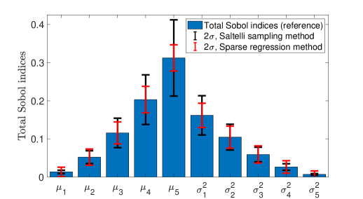
Figure 2: Total Sobol’ indices of $P_{\bar{\tau}}$, with $\bar{\tau}=3$, from (7); the error bars illustrate the variability of the two sampling methods (Saltelli sampling and sparse regression PCE) around the reference values.

Figure 2 illustrates the higher accuracy, or lower variance, of PCE with sparse regression over Saltelli sampling: the standard deviation of the largest Sobol’ index is roughly 3 times smaller with sparse regression than it is with Saltelli sampling. This gap in accuracy appears to diminish for smaller indices, although the methods do not show comparable accuracy until the indices are below 0.1. As $P_{\bar{\tau}}$ can be expressed analytically, there may be additional benefits of the sparse regression method to be seen when one considers performing GSA on a rare event probability with noise due to sampling. We note that the total order of the PCE basis and the penalty parameter $\lambda$, which are user-defined parameters, can be changed without the need for additional runs of SS. These parameters can be cross validated in a post-processing step after the rare event simulation step, providing flexibility in this approach without adding any significant computational burden.

When combining PCE-based GSA with SS for estimating $P_{\bar{\tau}}(\boldsymbol{\xi})$, there is a tradeoff between the inner loop cost of estimating $P_{\bar{\tau}}$ via SS and the outer loop of aggregating $P_{\bar{\tau}}$ samples to build the PCE. In Figure 3, we separately vary $N_{\mathrm{SS}}$ and $N_{\mathrm{SAMP}}$ and examine the resulting distribution of the total Sobol’ indices, computed via sparse regression PCE. For a fixed $N_{\mathrm{SAMP}}$, we compute multiple realizations of the total indices for several values of $N_{\mathrm{SS}}$.

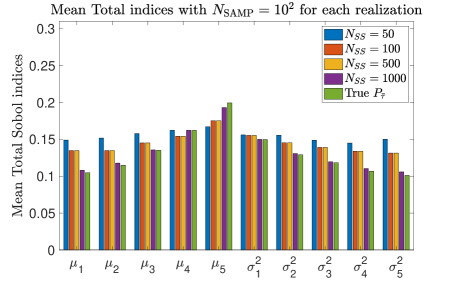
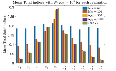
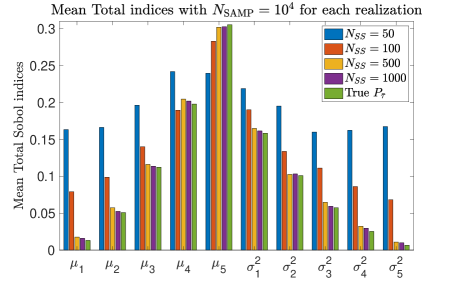
Figure 3: Mean Total Sobol’ indices, varying the computational cost of SS and the PCE construction. Each plot varies $N_{\mathrm{SAMP}}$ and each colored bar varies $N_{SS}$, with the final bar of each index corresponding to the analytic $P_{\bar{\tau}}$.

Figure 3 (top) displays the expected value of the total indices for $N_{\mathrm{SAMP}}=100$. Regardless of how accurately we estimate $P_{\bar{\tau}}$, the indices do not approach their true values because the PCE is built using an inadequate number of samples, resulting in a poor surrogate. By contrast, Figure 3 (middle) shows that for $N_{\mathrm{SAMP}}=10^{3}$, we only need a modest $N_{\mathrm{SS}}$ to approximate the Sobol’ indices. Indeed, for $N_{\mathrm{SS}}=500$, we are able to resolve the total indices very well. We also examine the case of $N_{\mathrm{SAMP}}=10^{4}$ in Figure 3 (bottom). Again, we are able to resolve the total indices well using only $N_{\mathrm{SS}}=500$ and are able to achieve the correct ordering for as little as $N_{\mathrm{SS}}=100$.

These results indicate that (i) a modest number of samples allocated to SS is enough to get a rough estimate of $P_{\bar{\tau}}$ and (ii) a moderate number of realizations of $P_{\bar{\tau}}(\boldsymbol{\xi})$ is then sufficient for accurate GSA. In other words, given rather poor estimations of $P_{\bar{\tau}}$, we are still able to extract accurate GSA results, due to the fact that the sparse regression technique is robust to noisy QoI evaluations.

5.2 Subsurface flow application

We consider the equations for single-phase, steady state flow in a square domain $\mathcal{D}=[0,1]^{2}$:

$$-\nabla\cdotp\left(\frac{\kappa}{\mu}\nabla p\right) =0\quad\text{in}~{}\mathcal{D},$$ (18)

$$p =1\quad\text{on}~{}\Gamma_{1},$$

$$p =0\quad\text{on}~{}\Gamma_{2},$$

$$\nabla p\cdotp n =0\quad\text{on}~{}\Gamma_{3},$$

where $\kappa$ is the permeability, $\mu$ is the viscosity, and $p$ is the pressure. The boundaries $\Gamma_{1},\Gamma_{2}$, and $\Gamma_{3}$ indicate the left boundary, the right boundary, and the top/bottom boundaries, respectively. The Darcy velocity is defined as $\boldsymbol{v}=-\frac{\kappa}{\mu}\nabla p$. In the present study, we let $\mu=1$. The source of uncertainty in this problem is in the permeability field, which we model as a random field. We consider the flow of particles through the medium and focus on determining the probability that said particles do not reach the outflow boundary in a given amount of time. This problem has been used previously as a test problem for rare event estimation in [28] as it pertains to the long-term reliability of nuclear waste repositories. Our goal is to perform GSA with respect to the hyper-parameters that define the distribution law of the permeability field.

The statistical model for the permeability field

Following standard practice [28, 10], we model the permeability field as a log-Gaussian random field:

$$\log{\kappa}(x,\omega)=a(x,\omega)=\bar{a}(x)+\sigma_{a}z(x,\omega),$$ (19)

where $x\in\mathcal{D}$ and $\omega$ belongs to sample space that carries the random process. Here, $\bar{a}$ is the mean of the random field, $\sigma_{a}$ is a scalar which controls the pointwise variance of the field, and $z$ is a centered (zero-mean) random process. We let the covariance function of $z$ be given by

$$c_{z}(x,y)=\exp{\left(-\frac{|x_{1}-y_{1}|}{\ell_{x}}-\frac{|x_{2}-y_{2}|}{\ell_{y}}\right)},\quad x,y\in\mathcal{D},$$ (20)

where $\ell_{x}$ and $\ell_{y}$ denote the correlation lengths in horizontal and vertical directions. The random field is represented via a truncated Karhunan-Lòeve expansion (KLE):

$$a(x,\omega)\approx\bar{a}(x)+\sum_{k=1}^{\mathrm{N}_{\textsc{KL}}}\sqrt{\lambda_{k}}~{}\theta_{k}(\omega)~{}e_{k}(x).$$ (21)

In this representation, $\theta_{1},\ldots,\theta_{\mathrm{N}_{\textsc{KL}}}$ are independent standard normal random variables and $(\lambda_{i},e_{k})$, $k=1,\ldots,\mathrm{N}_{\textsc{KL}}$, are the leading eigenpairs of the covariance operator of the process. Our setup for the uncertain log-permeability field follows the one in [10]: we use permeability data from the Society for Petroleum Engineers [1] to define $\bar{a}$. Once we truncate the KLE, the random vector $\boldsymbol{\theta}=[\begin{matrix}\theta_{1}&\theta_{2}&\cdots&\theta_{\mathrm{N}_{\textsc{KL}}}\end{matrix}]^{\top}$ fully describes the uncertainty in the log-permeability field.

To ensure that the KLE accurately models the variability of the infinite-dimensional field, we examine the eigenvalue decay of the covariance operator with the goal to truncate the KLE so that at least 90% of the average variance of the field is maintained. For $\ell_{x}=\ell_{y}=0.4$, which are the smallest correlation lengths considered in the present study, we require at least $\mathrm{N}_{\textsc{KL}}=126$. The number of retained KL modes then determines the dimensionality of the rare event estimation problem, and is henceforth fixed at $126$. The dimension independent properties of SS is advantageous in this regime.

For illustration, we plot two realizations of the random field, with the corresponding pressure and velocity fields obtained by solving the governing PDE (18), in Figure 4. In our computations, we solve the PDE using piecewise linear finite elements in Matlab’s finite element toolbox with 50 mesh points in each direction.

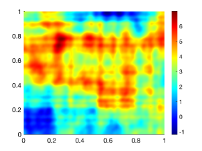
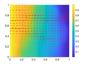
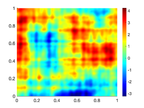
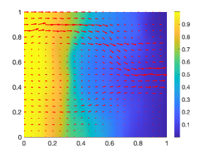
Figure 4: Left: plots showing two realizations of the log permeability field. Right: the corresponding pressure solution and arrows indicating the resulting Darcy velocity field.

The QoI and rare events under study

The position $\boldsymbol{x}$ of a particle moving with the flow through the medium is determined by the following ODE

$$\frac{d\boldsymbol{x}}{dt} =\boldsymbol{v},$$ (22)

$$\quad\boldsymbol{x}(0) =\boldsymbol{x}_{0},$$

where $\boldsymbol{v}$ is the Darcy velocity. We consider a single particle with initial position at $\boldsymbol{x}_{0}=\begin{bmatrix}0\\ 0.5\end{bmatrix}$. The solution $\boldsymbol{x}$ of (22) depends not only on time but also on $\boldsymbol{\theta}$ due to dependence of $\boldsymbol{v}$ on $\boldsymbol{\theta}$, i.e., $\boldsymbol{x}=\boldsymbol{x}(t,\boldsymbol{\theta})$. We take the QoI $q$ as the hitting time, i.e., the time it takes a particle to travel through the medium from left to right

$$q(\boldsymbol{\theta})=\{t:x_{1}(t,\boldsymbol{\theta})=1\}.$$

We aim to determine the rare event probability $P_{\bar{\tau}}=\mathbb{P}(q>\bar{\tau})$. The parameters $\ell_{x}$, $\ell_{y}$, and $\sigma_{a}$ parametrize the uncertainty in the permeability field; we consider them as hyper-parameters and set $\boldsymbol{\xi}=[\begin{matrix}\ell_{x}&\ell_{y}&\sigma_{a}\end{matrix}]^{\top}$. We set the nominal values of the hyper-parameters $\boldsymbol{\xi}_{nom}=[\begin{matrix}0.4&0.4&0.8\end{matrix}]^{\top}$. We simulate realizations of the permeability field at these nominal hyper-parameters and plot the distribution of $q$. Each of these realizations requires one PDE solve and one ODE solve.

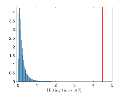
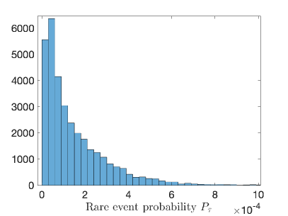
Figure 5: Left: Histogram of $q$ for nominal hyper-parameters. Vertical line indicates rare event threshold of $\bar{\tau}=4.5$. Right: histogram of the rare event probability, estimated via SS with uniformly distributed hyper-parameters.

As illustrated in Figure 5, the distribution for $q$ corresponds to a heavy-tailed distribution. We select as the threshold $\bar{\tau}=4.5$ and consider quantifying the sensitivity of $P_{\bar{\tau}}(\boldsymbol{\xi})$ with respect to the hyper-parameters defining the KLE.

Rare event probabilities and GSA

In our first set of experiments, we use SS with $N_{SS}=10^{3}$ samples per intermediate level; each of these samples corresponds to one solution of the full subsurface flow problem, including a PDE and ODE solve. For each evaluation of SS, approximately 5 intermediate levels are used, resulting in approximately $5\times 10^{3}$ function evaluations. Our hyper-parameters are drawn from a uniform distributed centered at $\boldsymbol{\xi}_{nom}$ with a spread of plus or minus 10% of $\boldsymbol{\xi}_{nom}$. We use these SS estimations of $P_{\bar{\tau}}(\boldsymbol{\xi})$ in order to build the corresponding PCE surrogate, where the polynomial basis is truncated at a total polynomial order of 5. Note the decision of where to truncate the PCE basis does not need to be made prior to estimating the set of $P_{\bar{\tau}}(\boldsymbol{\xi})$ samples.

The samples for the hyper-parameters are drawn using a Latin hypercube sampling scheme. We use $10^{3}$ estimations of $P_{\bar{\tau}}(\boldsymbol{\xi})$ to construct the PCE surrogate. Again, we use sparse regression to recover the PCE coefficients, while promoting sparsity in the set of PCE coefficients, and so mitigating the effects of noise induced by SS.

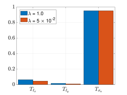
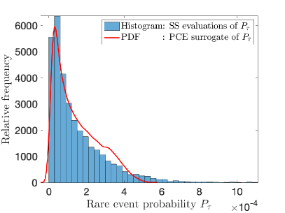
Figure 6: Left: total Sobol’ indices for $P_{\bar{\tau}}(\boldsymbol{\xi})$ computed from recovered PCE coefficients; results are reported with regularization constant $\lambda=1$ and $\lambda=5\times 10^{-2}$. Right: PDF of PCE surrogate compared with $P_{\bar{\tau}}$ evaluation histogram. Used $\mathrm{N}_{\textsc{samp}}=10^{4}$ for better resolution of distributions.

In Figure 6, we use two different values of $\lambda$ when promoting sparsity in order to illustrate the effect of $\lambda$ on the results. Note that when $\lambda$ is made smaller, the PCE coefficients decrease in magnitude, promoting a sparser PCE spectrum. In both cases, the ordering of the total Sobol’ indices remains consistent, and thus, conclusions with respect to parameter sensitivity are unaffected. For this experiment, we therefore conclude that choosing $\lambda$ by trial and error is sufficient. Should one encounter a scenario where the GSA results are more sensitive to $\lambda$, more systematic approaches are possible [7, 15].

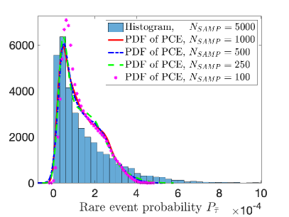
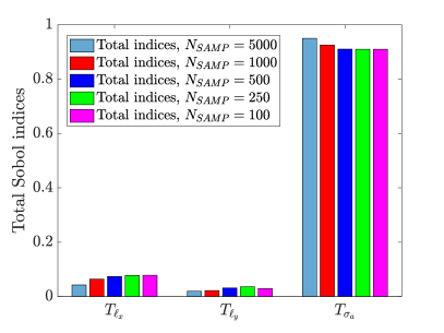
Figure 7: Distributions of $P_{\bar{\tau}}$ for $\mathrm{N}_{\text{SS}}=500$ and varying values of $\mathrm{N}_{\textsc{samp}}$. For each $\mathrm{N}_{\textsc{samp}}$, we build the PCE surrogate and approximate its PDF with $10^{5}$ samples. The set of $P_{\bar{\tau}}$ samples used for differing $\mathrm{N}_{\textsc{samp}}$ is nested within sets of larger samples. Corresponding total indices are included, computed directly from the PCE surrogates.

We lastly return to the key point made in Section 5.1, that the proposed method is capable of producing reliable GSA results, while using a modest number of inner and outer loop samples ($\mathrm{N}_{\text{SS}}$ and $\mathrm{N}_{\textsc{samp}}$, respectively). In Figure 7, we report results corresponding to $\mathrm{N}_{\text{SS}}=500$. In the left panel of the Figure we study the effect of $\mathrm{N}_{\textsc{samp}}$ on the PDF of the PCE surrogate. In the right panel, we plot the Sobol’ indices corresponding to each of the computed surrogates. The results in Figure 7 should also be compared with those in Figure 6, where larger values of $\mathrm{N}_{\text{SS}}$ and $\mathrm{N}_{\textsc{samp}}$ were used. This experiment indicates that $P_{\bar{\tau}}$ and the Sobol’ indices themselves can be well-approximated with a modest number of samples in both the inner and outer loops. In this case, using both $\mathrm{N}_{\text{SS}}$ and $\mathrm{N}_{\textsc{samp}}$ on the order of $10^{2}$ is sufficient for obtaining accurate GSA results. The combined cost of this method is thus reduced by a significant margin compared with the similar results in Figure 6. The efficiency gains of this method indicate the potential for deployment on problems which would otherwise be intractable.

6 Conclusion and future work

We have shown that the feasibility of the standard double-loop approach for GSA of rare event probabilities can be significantly extended beyond simple applications. This requires appropriate acceleration methods; in our case, this is achieved through subset simulation and the choice of a surrogate model allowing for the analytical calculation of Sobol’ indices. This approach is conceptually simple and does not require the development of new, ad hoc sensitivity concepts. While we have extended the range of applicability of the double-loop approach, we acknowledge that more research is needed to deal with computationally expensive, high-dimensional problems.

The efficiency of our method crucially depends on working with surrogate models for which sensitivity measures — here, Sobol’ indices — can be computed cheaply or “for free”; this clearly and strongly limits the type of GSA which can be carried out by the approach. More generally, if $q$ is the original QoI and if $\tilde{q}$ is the resulting QoI for a given surrogate model, more work is needed to understand the relationship between the approximation error $q-\tilde{q}$ and the resulting GSA error $\mathcal{S}(q)-\mathcal{S}(\tilde{q})$ where $\mathcal{S}(\cdot)$ is some sensitivity measure; more explicitly, there may be room for the development “cheap” surrogate models with moderate approximation errors and small GSA errors. Additionally, both our sensitivity analysis method as well as surrogate modeling approach rely on the assumption that the hyper-parameters are independent. In some cases one might be interested in GSA of rare event probabilities to both hyper-parameters and additional parameters in a model that might be uncertain and possibly correlated. Therefore, another interesting line of inquiry is to consider GSA of rare event probability with respect to correlated parameters. Further study may also include extensions of our approach to other moment-based QoIs (e.g. CDF approximation, skewness, kurtosis) and the use of perturbation-based methods for GSA [17] as opposed to considering a discrete set of hyper-parameters.

Acknowledgements

This research was supported by NSF through grants DMS 1745654 and DMS 1953271 and the US Dept. of Energy (DOE) through Sandia National Laboratories.

References

- spe [2000] 2001 SPE comparative solution project., 2000. URL https://www.spe.org/web/csp/datasets/set02.htm.
- Alexanderian [2013] Alen Alexanderian. On spectral methods for variance based sensitivity analysis. Probability Surveys, 10:51–68, 2013.
- Asmussen and Glynn [2007] Søren Asmussen and Peter W Glynn. Stochastic simulation: algorithms and analysis, volume 57. Springer Science & Business Media, 2007.
- Au and Beck [2001] Siu-Kui Au and James L Beck. Estimation of small failure probabilities in high dimensions by subset simulation. Probabilistic engineering mechanics, 16(4):263–277, 2001.
- Beck and Zuev [2017] James L. Beck and Konstantin M. Zuev. Rare-event simulation. In Handbook of uncertainty quantification. Vol. 1, 2, 3, pages 1075–1100. Springer, Cham, 2017.
- Bhatia and Davis [2000] Rajendra Bhatia and Chandler Davis. A better bound on the variance. The american mathematical monthly, 107(4):353–357, 2000.
- Blatman and Sudret [2010] Géraud Blatman and Bruno Sudret. Efficient computation of global sensitivity indices using sparse polynomial chaos expansions. Reliab. Eng. Syst. Safe., 95(11):1216–1229, 2010.
- Chabridon [2018] Vincent Chabridon. Reliability-oriented sensitivity analysis under probabilistic model uncertainty–Application to aerospace systems. PhD thesis, Université Clermont Auvergne, 2018.
- Chabridon et al. [2018] Vincent Chabridon, Mathieu Balesdent, Jean-Marc Bourinet, Jérôme Morio, and Nicolas Gayton. Reliability-based sensitivity estimators of rare event probability in the presence of distribution parameter uncertainty. Reliability Engineering & System Safety, 178:164–178, 2018.
- Cleaves et al. [2019] Helen L Cleaves, Alen Alexanderian, Hayley Guy, Ralph C Smith, and Meilin Yu. Derivative-based global sensitivity analysis for models with high-dimensional inputs and functional outputs. SIAM Journal on Scientific Computing, 41(6):A3524–A3551, 2019.
- Crestaux et al. [2009] Thierry Crestaux, Olivier Le Maıtre, and Jean-Marc Martinez. Polynomial chaos expansion for sensitivity analysis. Reliability Engineering & System Safety, 94(7):1161–1172, 2009.
- Dupuis et al. [2020] Paul Dupuis, Markos A Katsoulakis, Yannis Pantazis, and Luc Rey-Bellet. Sensitivity analysis for rare events based on rényi divergence. The Annals of Applied Probability, 30(4):1507–1533, 2020.
- Ehre et al. [2020] Max Ehre, Iason Papaioannou, and Daniel Straub. A framework for global reliability sensitivity analysis in the presence of multi-uncertainty. Reliability Engineering & System Safety, 195:106726, 2020.
- Fajraoui et al. [2017] Noura Fajraoui, Stefano Marelli, and Bruno Sudret. Sequential design of experiment for sparse polynomial chaos expansions. SIAM/ASA Journal on Uncertainty Quantification, 5(1):1061–1085, 2017.
- Hampton and Doostan [2017] Jerrad Hampton and Alireza Doostan. Compressive sampling methods for sparse polynomial chaos expansions. In Handbook of uncertainty quantification, pages 827–855. Springer International Publishing, 2017.
- Le Maître and Knio [2010] Olivier Le Maître and Omar M Knio. Spectral methods for uncertainty quantification: with applications to computational fluid dynamics. Springer Science & Business Media, 2010.
- Lemaître et al. [2015] Paul Lemaître, Ekatarina Sergienko, Aurélie Arnaud, Nicolas Bousquet, Fabrice Gamboa, and Bertrand Iooss. Density modification-based reliability sensitivity analysis. Journal of Statistical Computation and Simulation, 85(6):1200–1223, 2015.
- Li and Xiu [2010] Jing Li and Dongbin Xiu. Evaluation of failure probability via surrogate models. Journal of Computational Physics, 229(23):8966–8980, 2010.
- Li et al. [2011] Jing Li, Jinglai Li, and Dongbin Xiu. An efficient surrogate-based method for computing rare failure probability. Journal of Computational Physics, 230(24):8683–8697, 2011.
- Melchers and Beck [2018] Robert E Melchers and André T Beck. Structural reliability analysis and prediction. John wiley & sons, 2018.
- Morio [2011] Jérôme Morio. Influence of input pdf parameters of a model on a failure probability estimation. Simulation Modelling Practice and Theory, 19(10):2244–2255, 2011.
- Papaioannou et al. [2015] Iason Papaioannou, Wolfgang Betz, Kilian Zwirglmaier, and Daniel Straub. MCMC algorithms for subset simulation. Probabilistic Engineering Mechanics, 41:89–103, 2015.
- Peherstorfer et al. [2017] Benjamin Peherstorfer, Boris Kramer, and Karen Willcox. Combining multiple surrogate models to accelerate failure probability estimation with expensive high-fidelity models. Journal of Computational Physics, 341:61–75, 2017.
- Saltelli et al. [2010] Andrea Saltelli, Paola Annoni, Ivano Azzini, Francesca Campolongo, Marco Ratto, and Stefano Tarantola. Variance based sensitivity analysis of model output. design and estimator for the total sensitivity index. Comput. Phys. Commun., 181:259–270, 2010.
- Schuëller et al. [2004] GI Schuëller, HJ Pradlwarter, and Phaedon-Stelios Koutsourelakis. A critical appraisal of reliability estimation procedures for high dimensions. Probabilistic engineering mechanics, 19(4):463–474, 2004.
- Šehić and Karamehmedović [2020] Kenan Šehić and Mirza Karamehmedović. Estimation of failure probabilities via local subset approximations. arXiv preprint arXiv:2003.05994, 2020.
- Tong et al. [2020] Shanyin Tong, Eric Vanden-Eijnden, and Georg Stadler. Extreme event probability estimation using pde-constrained optimization and large deviation theory, with application to tsunamis. arXiv preprint arXiv:2007.13930, 2020.
- Ullmann and Papaioannou [2015] Elisabeth Ullmann and Iason Papaioannou. Multilevel estimation of rare events. SIAM/ASA Journal on Uncertainty Quantification, 3(1):922–953, 2015.
- van den Berg and Friedlander [2019] E. van den Berg and M. P. Friedlander. SPGL1: A solver for large-scale sparse reconstruction, December 2019. https://friedlander.io/spgl1.
- Wang et al. [2021] Pan Wang, Chunyu Li, Fuchao Liu, and Hanyuan Zhou. Global sensitivity analysis of failure probability of structures with uncertainties of random variable and their distribution parameters. Engineering with Computers, pages 1–19, 2021.
- Wang and Jia [2020] Zhenqiang Wang and Gaofeng Jia. Augmented sample-based approach for efficient evaluation of risk sensitivity with respect to epistemic uncertainty in distribution parameters. Reliability Engineering & System Safety, 197:106783, 2020.
- Zuev et al. [2012] Konstantin M Zuev, James L Beck, Siu-Kui Au, and Lambros S Katafygiotis. Bayesian post-processor and other enhancements of subset simulation for estimating failure probabilities in high dimensions. Computers & structures, 92:283–296, 2012.