The Integrated Sachs Wolfe effect: unWISE and Planck constraints on Dynamical Dark Energy

Abstract

CMB photons redshift and blueshift as they move through gravitational potentials $\Phi$ while propagating across the Universe. If the potential is not constant in time, the photons will pick up a net redshift or blueshift, known as the Integrated Sachs-Wolfe (ISW) effect. In the $z\ll 1000$ universe, $\dot{\Phi}$ is nonzero on large scales when the Universe transitions from matter to dark energy domination. This effect is only detectable in cross-correlation with large-scale structure at $z\sim 1$. In this paper we present a 3.2$\sigma$ detection of the ISW effect using cross-correlations between unWISE infrared galaxies and Planck CMB temperature maps. We use 3 tomographic galaxy samples spanning $0<z<2$, allowing us to fully probe the dark energy domination era and the transition into matter domination. This measurement is consistent with $\Lambda$CDM ($A_{\rm ISW}=0.96\pm 0.30$). We study constraints on a particular class of dynamical dark energy models (where the dark energy equation of state is different in matter and dark energy domination), finding that unWISE-ISW improves constraints from type Ia supernovae due to improved constraints on the time evolution of dark energy. When combining with BAO measurements, we obtain the tightest constraints on specific dynamical dark energy models. In the context of a phenomenological model for freezing quintessence, the Mocker model, we constrain the dark energy density within 10% at $z<2$ using ISW, BAO and supernovae. Moreover, the ISW measurement itself provides an important independent check when relaxing assumptions about the theory of gravity, as it is sensitive to the gravitational potential rather than the expansion history.

1 Introduction

On super-horizon scales ($\ell<200$) the cosmic microwave background (CMB) power spectrum is dominated by the Sachs-Wolfe effect [1, 2]. On these scales, fluctuations in the gravitational potential generate fluctuations in the CMB as photons exiting the potentials are redshifted and blueshifted. For adiabatic fluctuations in a matter-dominated universe, the temperature fluctuations generated by the Sachs-Wolfe effect are

$$\frac{\Delta T}{T}=-\frac{1}{3}\Phi$$ (1.1)

where the factor of $-1/3$ comes from gravitational redshifting as photons exit the potential (contributing $-\Phi$) and clocks running slow within the gravitational potential (contributing $2\Phi/3$) [1, 3]. Since the dimensionless angular power spectrum of potential fluctuations is flat, this creates a characteristic “Sachs-Wolfe plateau” at low $\ell$ in the primary CMB.

The Integrated Sachs-Wolfe effect is an additional effect from the time dependence of the gravitational potential as photons propagate through the observable universe, from the surface of last scattering to the observer on Earth. In matter domination and in the linear regime, gravitational potentials are constant in time, so photons redshift in and out of potentials with no effect. However, the gravitational potential decays during dark energy domination, and this leads to a net blueshift of photons as they travel through decaying potentials. This effect is too small to be detectable in the CMB power spectrum, but is detectable in cross-correlation with large-scale structure.

Since the ISW effect in linear theory is only sourced by dark energy, it is a powerful direct probe of it, complementary to measurements based on the distance-redshift relation, matter clustering, and the primary CMB [4, 5, 6]. Moreover, while often measurements are “integrated” over a large redshift range, the dependence of ISW on $\dot{\Phi}$ at the redshift of the measurement only can be more sensitive to variations in dark energy properties over relatively narrow redshift ranges. As a result, measurements of the ISW effect can test dark energy [7] and probe extensions to $\Lambda$CDM such as modified gravity [8, 9] or spatial curvature [10].

On nonlinear scales, even during matter domination, gravitational potentials are not constant in time. This additional nonlinear integrated Sachs-Wolfe effect is also known as the Rees-Sciama effect [2, 11] but it is generally too small to detect with the current generation of surveys, and is found at larger $\ell$ than considered here. In addition, a time-varying potential is also generated by the galaxy motion across the line of sight [12], an effect known as “moving lens” or “slingshot”. This component of the signal and its detectability has been studied in [13, 14, 15, 16, 17, 18], and we note that a simple cross-correlation between galaxy positions and the CMB fluctuations will not receive a contribution from the “moving lens” effect, and therefore we won’t consider it here.

Since the first detection of the ISW cross-correlation by Ref. [19], there have been many ISW detections with a variety of galaxy samples and CMB data from WMAP [20, 21, 22, 23, 24, 25, 26, 27, 28, 29, 30, 31, 32, 33, 34, 35, 36] and Planck [37, 38, 39, 40, 41]. The highest significance detections range from 4–5$\sigma$ [42, 38, 39]. These measurements have been used to constrain cosmological parameters and dark energy, including the curvature of the universe and the dark energy equation of state [22, 43, 29, 25, 42, 30, 44, 45, 46].

The unWISE catalog [47] is ideal for an ISW cross-correlation measurement. It contains $\sim 500$ million galaxies across the entire sky out to $z\sim 2$, covering the entire dark-enegy dominated epoch. The sky and redshift coverage are ideal for overlap with the ISW kernel. Additionally, we split the sample into three redshift bins using the unWISE galaxies’ infrared colors, allowing us to probe the ISW tomographically.

Type Ia supernovae and baryon acoustic oscillations (BAO) generally constrain dark energy at $z<1$, leaving the dark energy equation of state at higher redshift relatively unconstrained. Tomography over the range $0\lesssim z\lesssim 2$ is particularly interesting in light of the reported ISW “anomalies” obtained when stacking on supersclusters and supervoids, where an anomalous signal is found [48, 49, 50], and the size (as well as the sign) of this discrepancy evolves quite rapidly over this redshift range. For example, there have been hints of a negative ISW signal at $z\sim 1.5$ [50], which should leave an imprint in our measurement out to $z=2$.

To demonstrate how this ISW measurement improves our knowledge of dark energy at $z>1$, we consider constraints on dynamical dark energy models, i.e. models where the dark energy equation of state changes at $z\sim 1-2$ (see for example [51, 52, 53]). These are sometimes referred to in the literature as “early dark energy” models but should not be confused with models postulating an additional dark energy component in the $z\sim 1000$ universe in order to address the Hubble tension [54, 55, 56, 57, 58]. To avoid confusion, we will refer to the models with dark energy decaying at $z\sim 1-2$ as “dynamical dark energy” throughout this paper.

The outline of the paper is as follows. We describe the theory in Section 2, summarize the data used in Section 3, describe the methodology of the ISW cross-correlation measurement in Section 4, and present the measurement and compare to $\Lambda$CDM and a freezing quintessence model for dynamical dark energy in Section 5. Where necessary we assume a fiducial $\Lambda$CDM cosmology with the Planck 2018 maximum likelihood parameters, $\Omega_{m}=0.3096$, $H_{0}=67.66$, $n_{s}=0.9665$, $\sigma_{8}=0.8102$, $\Omega_{b}=0.049$, and one massive neutrino with mass 0.06 eV. We quote magnitudes in the Vega system, noting that we can easily convert these to AB magnitudes with AB = Vega + 2.699, 3.339 in W1, W2, respectively.

2 Theory

The integrated Sachs-Wolfe effect comes from the blueshifting of CMB photons due to a changing gravitational potential

$$\left(\frac{\Delta T}{T}\right)_{\rm ISW}=-2\int d\chi\ e^{-\tau}\dot{\Phi}$$ (2.1)

where the factor of 2 comes from the fact that both the spatial and time components of the perturbed potential contribute to the ISW effect, $\chi$ is the comoving distance, $\tau$ is the optical depth to distance $\chi$ and the dot refers to derivative with respect to conformal time. Since we will only work with low redshift samples, we can neglect the $e^{-\tau}$ term and set it to 1. In the linear regime and after recombination, $\dot{\Phi}$ is only nonzero in dark energy domination.

Since the ISW is the only physical correlation between foreground galaxies and CMB temperature at low $\ell$, the cross-power spectrum $C_{\ell}^{Tg}$ is given by

$$C_{\ell}^{Tg}=C_{\ell}^{\dot{\Phi}g}=\frac{2}{\pi}\int\,k^{2}\,dk\,P(k)K_{\ell}^{\dot{\Phi}}(k)\,K_{\ell}^{g}(k)$$ (2.2)

The kernel functions $K_{\ell}^{\dot{\Phi}}(k)$ and $K_{\ell}^{g}(k)$ are

$$K_{\ell}^{g}(k)=\int\,dz\,b(z)\frac{dN}{dz}D(z)\,j_{\ell}[k\chi(z)]$$ (2.3)

$$K_{\ell}^{\dot{\Phi}}(k)=\frac{3\Omega_{m}H_{0}^{2}}{k^{2}}\int dz\,\frac{d}{dz}\left[(1+z)D(z)\right]\,j_{\ell}[k\chi(z)]$$ (2.4)

where $dN/dz$ is the galaxy redshift distribution, $b(z)$ is the bias evolution, $D(z)$ is the linear growth factor, and $j_{\ell}$ are spherical Bessel functions. We compare the ISW sensitivity, $\frac{d[(1+z)D(z)]}{dz}\frac{dV}{dz}$, to the redshift distribution of the unWISE galaxies in Fig. 1.

We also consider the cross-correlation between the ISW and cosmic magnification, $C_{\ell}^{\dot{\Phi}\mu}$

$$C_{\ell}^{T\mu}=C_{\ell}^{\dot{\Phi}\mu}=\frac{2}{\pi}\int\,k^{2}\,dk\,P(k)K_{\ell}^{\dot{\Phi}}(k)\,K_{\ell}^{\mu}(k)$$ (2.5)

with kernel $K_{\ell}^{\mu}(k)$

$$K_{\ell}^{\mu}(k)=(5s-2)\,\frac{3}{2}\Omega_{m}H_{0}^{2}\int dz\,(1+z)g_{i}(\chi(z))D(z)j_{\ell}[k\chi(z)]$$ (2.6)

where $s$ is the response of the number density to magnification, and

$$g_{i}(\chi)=\int_{\chi}^{\chi_{\star}}d\chi^{\prime}\ \frac{\chi(\chi^{\prime}-\chi)}{\chi^{\prime}}\ H(z^{\prime})\ \frac{dN_{i}}{dz^{\prime}}$$ (2.7)

For the green and red samples, $s$ is large enough that magnification bias makes a substantial contribution to the observed unWISE-CMB temperature cross-correlation (Fig. 2).

Note that Eqs. 2.2–2.4 are only valid in the linear regime where the power spectrum $P(k,z)$ can be separated into $P(k)$ and $D(z)$. To improve accuracy at higher $\ell$, we instead use the nonlinear $P(k)$ [60, 41] from HALOFIT [61], although we find this makes very little difference on the large scales we consider. We use CAMBSources [62], part of the CAMB package [63, 64], to compute $C_{\ell}^{Tg}$.

3 Data

3.1 unWISE

3.1.1 Galaxy catalog

The WISE mission mapped the entire sky at 3.4, 4.6, 12 and 22 $\mu$m (W1, W2, W3, and W4), with angular resolutions of 6.1”, 6.4”, 6.5” and 12”, respectively [65]. The original mission collected data in 2010. After a two year hibernation, the satellite was reactivated and continued observations as NEOWISER (NEOWISE-Reactivation) [66, 67] and has been continuously mapping the sky in W1 and W2 since 2014. The unWISE catalog was created from the first five years of imaging: one year of WISE and four from NEOWISE [68, 69, 70, 71]. It reaches 0.7 mags deeper than the AllWISE catalog from 2010.

The W1 and W2 magnitudes enable us to roughly divide the sample by redshift, yielding 3 samples spanning $0<z<2$. Additionally, we use Gaia to remove stars from the sample, yielding residual stellar contamination of $\sim 2\%$ as measured by deep imaging in the COSMOS field [72]. These samples were characterized and used in Ref. [47, 73, 74], and we refer the reader to Ref. [73] for a more comprehensive discussion. We reproduce Table 1 from Refs. [73, 74] to summarize the important properties of the sample: the color selection, redshift distribution, number density, galaxy bias, and response of number density to galaxy magnification $s\equiv d\log_{10}N/dm$. We measure $s$ using galaxies with ecliptic latitude $|\lambda|>60^{\circ}$, where the WISE depth of coverage is greater and thus the measurement of $s$ is less affected by incompleteness (see discussion in Appendix D in Ref. [73]).

Label	$\mathrm{W1}-\mathrm{W2}>x$	$\mathrm{W1}-\mathrm{W2}<x$	$\mathrm{W2}<x$	$\bar{z}$	$\delta z$	$\bar{n}$	$s$	$b^{\rm eff}\pm\textrm{stat}\pm\textrm{$dN/dz$}$
Blue		$(17-\mathrm{W2})/4+0.3$	16.7	0.6	0.3	3409	0.455	$1.50\pm 0.025\pm 0.037$
Green	$(17-\mathrm{W2})/4+0.3$	$(17-\mathrm{W2})/4+0.8$	16.7	1.1	0.4	1846	0.648	$2.23\pm 0.032\pm 0.025$
Red	$(17-\mathrm{W2})/4+0.8$		16.2	1.5	0.4	144	0.842	$3.19\pm 0.076\pm 0.059$

Table 1: WISE Color and magnitude cuts for selecting unWISE galaxies of different redshifts, together with the mean redshift, $\bar{z}$, and the width of the redshift distribution, $\delta z$ (as measured by matching to objects with photometric redshifts on the COSMOS field [75]); number density per deg² within the unWISE mask, $\bar{n}$; response of the number density to magnification, $s\equiv d\log_{10}N/dm$; and average bias $b^{\rm eff}$ (Eq. 3.3) along with its statistical and systematic errors from uncertainty in the redshift distribution. Galaxies are additionally required to have $\mathrm{W2}>15.5$, to be undetected or not pointlike in Gaia, and to not be flagged as diffraction spikes, latents or ghosts. See Refs. [47, 73, 74] for further details.

We require that the blue and green samples have $15.5<\mathrm{W2}<16.7$, and the red sample has $15.5<\mathrm{W2}<16.2$; in Ref. [73] we find that deeper red samples are potentially affected by systematics.

We remove potentially spurious sources (diffraction spikes, latents, ghosts) and all galaxies are required to be either undetected or not pointlike in Gaia. Here a source is taken as “pointlike” if

$$\mathrm{pointlike}(G,A)=\begin{cases}\log_{10}A<0.5&\text{if $G<19.25$}\\ \log_{10}A<0.5+\frac{5}{16}(G-19.25)&\text{otherwise}\,,\end{cases}$$ (3.1)

where G is the Gaia G band magnitude and $A$ is astrometric_excess_noise from Gaia DR2 [76]. A source is considered “undetected” in Gaia if there is no Gaia DR2 source within $2.75^{\prime\prime}$ of the location of the WISE source. High astrometric_excess_noise indicates that the Gaia astrometry of a source was more uncertain than typical for resolved sources; this cut essentially takes advantage of the $0.1^{\prime\prime}$ angular resolution of Gaia to morphologically separate point sources from galaxies. We estimate that this reduces the stellar contamination in our samples to $<2\%$.

The unWISE mask is based on the 2018 Planck lensing mask [77]. We additionally mask a small portion of the sky at $|b|<10^{\circ}$, and mask bright infrared stars, diffraction spikes, nearby galaxies, planetary nebulae, and low latitude pixels with a substantial number of fainter stars which will reduce the effective area in a pixel by masking galaxies within 2.75” of each star (due to the Gaia criterion). The full details of the mask construction are in section 2.3 of Ref. [73]; this mask yields $f_{\rm sky}=0.586$. Sky distributions of the masked unWISE galaxy samples are shown in Fig. 3.

We also create systematics weights for the unWISE galaxy samples to remove correlations with potentially contaminating large-scale systematics, such as Milky Way stellar density or WISE depth-of-coverage. We follow a similar methodology to the linear regression method used for SDSS and DES galaxy clustering analysis [78, 79, 80, 81, 82, 83, 84]. We start by creating HEALPix maps [85] at NSIDE=128 of the unWISE galaxy density field; stars from the Gaia catalog; unWISE W1 and W2 5$\sigma$ limiting magnitude; dust extinction $E(B-V)$ from the Schlegel-Finkbeiner-Davis map [86]; neutral hydrogen column density $N_{\textsc{HI}}$ from the H14PI survey [87]; and 3.5 and 4.9 $\mu$m sky brightness from the DIRBE Zodi-Subtracted Mission Average (ZSMA), and a separate estimate of the zodiacal background light from the DIRBE Sky and Zodi Atlas (DSZA) [88].

For the blue sample, we fit a linear trend between unWISE galaxy density and Gaia stellar density, and a piecewise linear trend to W2 5$\sigma$ limiting magnitude. We determine errorbars on each binned systematic property using the variance of density values from 100 Gaussian mocks with no correlation with the systematics templates. We find that correlations with all other templates (and residual correlations with stars and W2 depth) are $\lesssim 1\%$ after weighting. For green, the picture is similar, though we need to use a piecewise linear fit for both stellar density and W2 5$\sigma$ magnitude. Finally, for red we find that the most significant trends are to stellar density and $N_{\textsc{HI}}$, and fit piecewise linear trends to only these templates.

3.1.2 Bias and redshift distribution

Theory predictions for the ISW cross-correlation require both the redshift distribution of the galaxy sample, $dN/dz$, and its bias evolution $b(z)$ (Section 2). Our best-characterized measurement of the unWISE redshift distribution comes from cross-correlations with spectroscopic galaxies and quasars from SDSS [73]. The cross-correlation between unWISE and known spectroscopic galaxies in a narrow redshift bin at $z_{i}$ is proportional to the fraction of unWISE galaxies in that redshift bin, $dN/dz(z_{i})$, and the bias of the unWISE galaxies $z_{i}$, given that we can precisely measure the bias of the spectroscopic sample from its autocorrelation [89, 90, 91]. Repeating this using samples spanning the unWISE redshift range (e.g. galaxies and quasars from SDSS [92]) allows us to determine the bias-weighted redshift distribution $b(z)dN/dz$.

We normalize the cross-correlation redshift distribution to integrate to unity, and refer to the resulting quantity as $f(z)dN/dz$:

$$f(z)\frac{dN}{dz}\equiv\frac{b(z)\frac{dN}{dz}}{\int\,dz\,b(z)\frac{dN}{dz}}$$ (3.2)

Measurements of the product $f(z)dN/dz$ are convenient, because they appear together in the galaxy kernel in equation 2.3.

While we could use cross-correlations with spectroscopic samples to determine the amplitude of the bias evolution as well as $f(z)$, we instead use a simpler and more robust method: cross-correlations with gravitational lensing of the cosmic microwave background. Defining the effective bias $b^{\rm eff}$

$$b^{\rm eff}=\int\,dz\,b(z)\frac{dN}{dz}$$ (3.3)

in the Limber approximation, we may write the angular cross-correlation between the galaxies and CMB lensing as [73]

$$C_{\ell}^{\kappa g}=b^{\rm eff}\int d\chi\frac{W^{\kappa}(\chi)}{\chi^{2}}H(z)\left[f(z)\frac{dN}{dz}\right]P(k\chi=\ell\,+\,1/2)\\ +\int d\chi\frac{W^{\kappa}(\chi)W^{\mu}(\chi)}{\chi^{2}}P(k\chi=\ell\,+\,1/2)$$ (3.4)

In Table 1, we give the best-fit $b^{\rm eff}$ for each sample. The first set of errorbars are statistical error and the second set are error from uncertain $dN/dz$ (computed as the standard deviation of the best-fit bias from the 100 sampled $dN/dz$ as in Ref. [73]). The errors on the bias are at most 3%, and are thus negligible compared to the $\gtrsim 30\%$ errors on the ISW measurement (Table 2).

While the dominant terms in the ISW cross-correlation (Eq. 2.2) require $f(z)dN/dz$ rather than $dN/dz$, the lensing magnification terms are sensitive to $dN/dz$ alone. Here, we use the redshift distribution of unWISE galaxies matched to optical sources in the deep imaging of the 2 deg² COSMOS field. We use the multi-band photometric redshifts of Ref. [72], which have accuracy $\Delta z/(1+z)=0.007$ (referred to as “cross-match redshifts,” following [73]). The COSMOS imaging is sufficiently deep that nearly all of the unWISE galaxies have counterparts with photometric redshifts.

The cross-match redshifts are shifted to lower redshift than the cross-correlation redshifts (Fig. 1). We show in Ref. [73] that reconciling the cross-match and cross-correlation redshift distributions requires a bias evolution consistent with the observed evolution in the unWISE number density. We further construct in Ref. [74] a plausible Halo Occupation Distribution model that matches the COSMOS $dN/dz$, the clustering $f(z)dN/dz$, $C_{\ell}^{\kappa g}$ and $C_{\ell}^{gg}$. Therefore, we conclude that the COSMOS $dN/dz$ and clustering $f(z)dN/dz$ are consistent with each other.

Since the cross-correlation redshift distribution comes from noisy clustering measurements, the redshift distribution $f(z)dN/dz$ has uncertainty as well. We create samples of $f(z)dN/dz$ that are consistent with the data and whose density is proportional to their probability of being the correct one given the data. These samples are obtained by generating Gaussian random realizations with the correct noise covariance (one for each sample), adding the noise realization to the measured $f(z)dN/dz$, and finally fitting a smooth B-spline with positivity constraint and curvature penalty. The method is described further in Ref. [73], and also used in Ref. [74].

The cross-match redshift distribution is also noisy, with errors arising from uncertain photometric redshifts, sample variance, cosmic variance, and potentially variations in unWISE galaxy properties across the sky (since COSMOS is only 2 deg²). Due to the diverse sources of the noise, the uncertainties in cross-match $dN/dz$ are less well characterized. Moreover, as we show in Section 5, the uncertainty in $f(z)dN/dz$ is subdominant to the statistical uncertainty on the ISW measurement. Since the magnification terms sensitive to cross-match $dN/dz$ are smaller than the clustering terms sensitive to $f(z)dN/dz$, the contributions from uncertainty in $dN/dz$ are negligible compared to the statistical uncertainty.

An additional potential source of systematic error comes from the scale mismatch between the $C_{\ell}^{Tg}$ measurement and the cross-correlation redshift measurement. We measure the cross-correlation redshifts on fairly small scales (2.5 to 10 $h^{-1}$ Mpc in configuration space) so the bias will not be identical to the linear bias on large scales appropriate for ISW. It is therefore possible that the quasi-linear bias that we measure in the cross-correlation redshifts evolves differently with redshift as the linear bias. We construct simple HODs for the WISE sample [Appendix B in 73], and we can gain some understanding into the nonlinear bias evolution of the WISE sample using $N$-body simulations populated with these HODs. We find that the systematic shift and error from nonlinear bias evolution is smaller than the uncertainty from the measurement error in $dN/dz$. We optionally apply the “nonlinear bias correction,” derived from the HODs, as a correction to $f(z)\frac{dN}{dz}$ and find that it does not have a significant effect on the results.

3.2 Planck CMB data

We use the SMICA CMB temperature map from the Planck 2018 release as our fiducial temperature map in the ISW analysis. We use the common confidence mask (combined confidence mask for the different temperature pipelines) as described in Section 4.2 of Ref. [93]. SMICA produces a temperature map from a linear combination of the Planck input channels (30 to 857 GHz) with multipole-dependent weights, up to $\ell\sim 4000$. We repeat the measurement with the COMMANDER; NILC; SEVEM multi-frequency; SEVEM 70, 100, 143 and 217 GHz; and SMICA-noSZ maps to test the robustness of the result [93]. To measure the covariance, we use 300 FFP10 end-to-end simulations released as part of the Planck 2018 data release [94, 95, 93]. These simulations include instrumental noise, systematics, and foregrounds, and were processed with an identical pipeline to the data to produce component-separated maps.

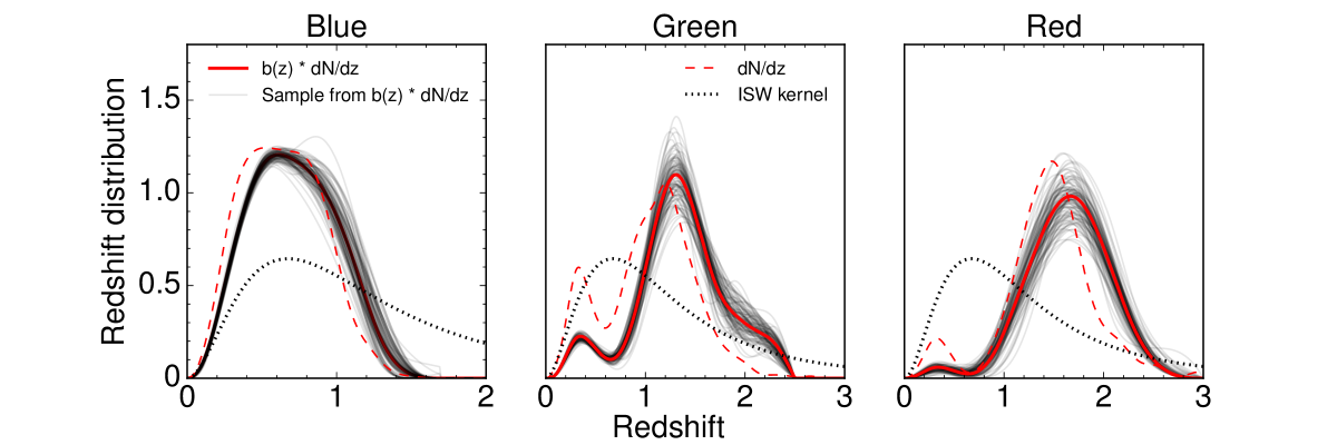
Figure 1: Redshift distributions of the 3 unWISE samples. The best measurement of the unWISE redshift distribution comes from cross-correlations with spectroscopic samples, which constrain the product of the bias evolution $b(z)$ and the redshift distribution $dN/dz$ (solid red lines). The cross-correlation redshift measurement is noisy and realizations of the uncertainty in $b(z)dN/dz$ are shown as the gray lines. We also show the redshift distribution $dN/dz$ as determined from cross-matching to multi-band photometric redshifts in the COSMOS field (red dashed line). $dN/dz$ enters in the ISW-magnification term (Eq. 2.5). As this term has a subdominant contribution to the overall signal, the uncertainties from uncertain $dN/dz$ are small and therefore not shown. The ISW kernel, $\frac{d[(1+z)D(z)]}{dz}\frac{dV}{dz}$, is shown as the black dotted line.

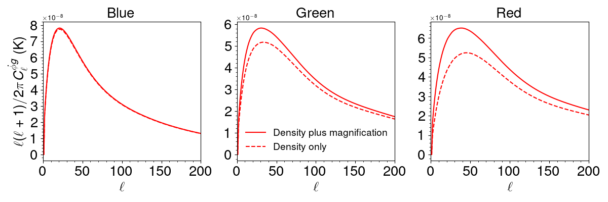
Figure 2: ISW-unWISE cross-correlation in the fiducial flat $\Lambda$CDM cosmology. The contributions from the density, $C_{\ell}^{\dot{\phi}g}$, and magnification $C_{\ell}^{\dot{\phi}\mu}$ are plotted separately. All of the other higher-order terms (i.e. redshift space distortions, peculiar velocity, time delay, source evolution, ISW, time delay; see ref. [62] for a complete discussion) change the total by $<2\%$ ($<0.3\%$ at $\ell>20$), and are largest for blue and red.

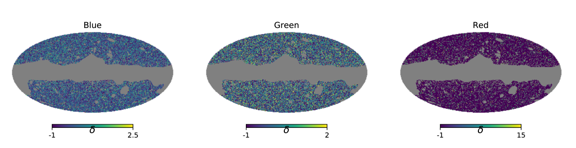
Figure 3: Sky distribution of the 3 unWISE samples, in Galactic coordinates.

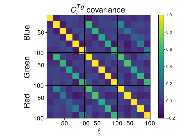
Figure 4: Correlation matrix of $C_{\ell}^{Tg}$, as determined by repeating the cross-correlation measurement on 300 Planck full-sky mocks and unWISE galaxy data. The bins shown are the fiducial ones used for the analysis; blue, green and red share 5 bins at $20<\ell<100$, and blue also uses an additional bin at $7<\ell<20$ which is omitted for green and red due to concerns about systematics in the galaxy sample.

For the CMB lensing cross-correlations used to measure $b^{\rm eff}$, we use the minimum-variance (MV) CMB lensing maps obtained from temperature and polarization SMICA maps from the Planck 2018 release. We mask the field with the mask provided by the Planck team. Our methodology closely follows Ref. [73] with two minor differences: we use $20<\ell<1000$ rather than $\ell_{\rm min}=100$ (as this conservative $\ell_{\rm min}$ is only necessary for the galaxy auto-correlation, which we do not use in this work); and we set $f(z)dN/dz$ to zero at $z>1.5$ (2.5, 3) for blue (green, red). Since the cross-match $dN/dz$ is nearly zero beyond these limits, any bumps in $f(z)dN/dz$ are likely to be noise.

4 Angular power spectrum measurement

In order to estimate the binned cross and auto power spectra, we use a pseudo-$C_{\ell}$ estimator [96] based on the harmonic coefficients of the galaxy and temperature fields. We follow the same procedure as in Ref. [73]. The measured pseudo-$C_{\ell}$ on the cut sky are calculated as

$$\tilde{C}_{\ell}^{XY}=\frac{1}{2\ell+1}\sum_{m}X_{\ell m}Y^{\star}_{\ell m}$$ (4.1)

where $X,Y\in\{g_{1},g_{2},g_{3},T,\kappa\}$ are the observed fields on the cut sky. Because of the mask, these differ from the true $C_{\ell}$ that are calculated from theory, but their expectation value is related through a mode-coupling matrix, $M_{\ell\ell^{\prime}}$, such that

$$\langle\tilde{C}_{\ell}\rangle=\sum_{\ell^{\prime}}M_{\ell\ell^{\prime}}C_{\ell^{\prime}}$$ (4.2)

The matrix $M_{\ell\ell^{\prime}}$ is purely geometric and can be computed from the power spectrum of the mask itself. While Eq. (4.2) is not directly invertible for all $\ell$, the MASTER algorithm [96] provides an efficient method to do so assuming that the power spectrum is piecewise constant in a number of discrete bins, $b$. Defining a “binned” mode-coupling matrix, $\mathcal{M}_{bb^{\prime}}$ [97], we can recover unbiased binned bandpowers

$$C_{b}=\sum_{b^{\prime}}\mathcal{M}^{-1}_{bb^{\prime}}\tilde{C}_{b^{\prime}}\quad.$$ (4.3)

We use the implementation in the code NaMaster [97].

We mask the galaxy map with the unWISE mask including bright stars and galaxies, and the CMB map with the “common” mask for CMB temperature, apodized with a Gaussian smoothing kernel with FWHM 1 degree. We also correct the unWISE density map by an “area lost” mask to account for the reduction in available area in each pixel due to point sources in Gaia (since we mask any source within 2.75” of a star). We test our pipeline on 100 noiseless Gaussian simulations (i.e. the CMB component is $C_{\ell}^{TT}$ from the late-time ISW only, and no galaxy shot-noise is added) to ensure that we recover the correct power spectrum. The binned theory spectrum is the dot product of the unbinned theory spectrum and bandpower window functions given by NaMaster. We check the bandpower window functions using Gaussian simulations and find that they are correct to within the Poisson measurement error on the simulations (Appendix A).

Since the azimuthal modes of the map are most affected by Galactic latitude-dependent foregrounds, we remove the $m=0$ mode from the sum in Eq. 4.1. This makes a very modest ($<0.25\sigma$) impact on our results, and we validate this procedure by omitting the $m=0$ modes in the Gaussian simulation test. Despite the omission of the $m=0$ mode, we find that the NaMaster bandpower window function describes the effect of binning very well.

We omit large-scale modes where the auto-spectrum of the unWISE galaxies deviates significantly from a theory model fit to smaller scales. We find that the auto-spectrum contains significant spurious power below $\ell=7$ for blue and $\ell=20$ for green and red. Thus we use bins at $7<\ell<100$ for blue and $20<\ell<100$ for green and red. For all samples, we use bins with width $\Delta\ell=16$ from $20<\ell<100$, and we add a bin at $7<\ell<20$ for blue. This is a conservative choice for $\ell_{\rm min}$, as the systematics in the galaxy map are likely not correlated with potential residual systematics in CMB temperature. Indeed we find that lowering $\ell_{\rm min}$ to 5 for the green sample leads to negligible changes in $A_{\rm ISW}$. However, since these modes are quite noisy, conservatively omitting them from the analysis makes little difference in our results. We omit modes at $\ell>100$, where the ISW signal is small, consistent with $\ell_{\rm max}$ commonly used in previous work [34, 36].

We use the 300 Planck simulations to determine the covariance of the ISW power spectra, including the cross-covariance between the different galaxy samples (Fig. 4). We apply our pipeline to measure the cross-correlation between each simulation and the unWISE maps, and then measure the covariance of these 300 power spectra. We apply the Hartlap correction to the inverse covariance matrix [98] to account for noise in the mock-based covariance, although this correction is tiny due to the small size of the data vector (5 bins). We find that the error bars from the Planck mocks are generally quite similar to the Gaussian error bars [99, 96, 100]. As a further check, we find that the error bars from the Planck mocks are generally similar to the scatter of the individual $C_{\ell}$ within each bin.

5 Comparison to theory

5.1 ISW measurement and comparison to $\Lambda$CDM

In Fig. 5, we show the measured ISW cross-correlation and the $\Lambda$CDM theory curve in the fiducial cosmology, multiplied by a scaling factor $A_{\rm ISW}$. Specifically, we bin the $C_{\ell}^{\dot{\Phi}-{\rm unWISE}}$ template identically to the data; multiply theory and measurement by $\ell_{\rm center}(\ell_{\rm center}+1)/2\pi$ to work with data that is roughly constant (where $\ell_{\rm center}$ is the center of each bin); and multiply the template by the bandpower window function (Fig. 8).

Fig. 5 demonstrates that our data is consistent with $\Lambda$CDM. We find $A_{\rm ISW}=0.73\pm 0.34$ for blue ($2.1\sigma$), $1.00\pm 0.39$ for green ($2.6\sigma$), and $1.14\pm 0.52$ for red ($2.2\sigma$), for a combined significance of $3.2\sigma$ (combined $A_{\rm ISW}=0.96\pm 0.30$), again using the 300 FFP10 simulations to calculate the correct covariances between the individual ISW cross-correlations. The $\Lambda$CDM model ($A_{\rm ISW}$ = 1) provides a good fit to the data, with $\chi^{2}=10.4$ over 15 degrees of freedom.

The significance of detection for the blue sample is somewhat lower than previous expections. Ref. [101] expects signal-to-noise of $\sim 5$ for an $f_{\rm sky}=0.6$ survey with 100 million galaxies out to $z_{\rm max}=1$, with bias of 1.5. However, our $\ell_{\rm min}=7$ cut reduces the signal-to-noise by $\sim 20$% (the $\ell_{\rm max}=100$ cut makes $<2\%$ difference). Furthermore, even with the $\ell_{\rm min}$ cut, the autocorrelation of the blue sample is higher than the $\Lambda$CDM expectation (presumably due to uncorrected systematics). Without this excess noise at low $\ell$, an ISW signal with $A_{\rm ISW}=1$ would be detected at 3.7$\sigma$ (versus $1/0.34=2.9\sigma$ from Table 2). This is quite consistent with the 4$\sigma$ detection expected from Ref. [101].

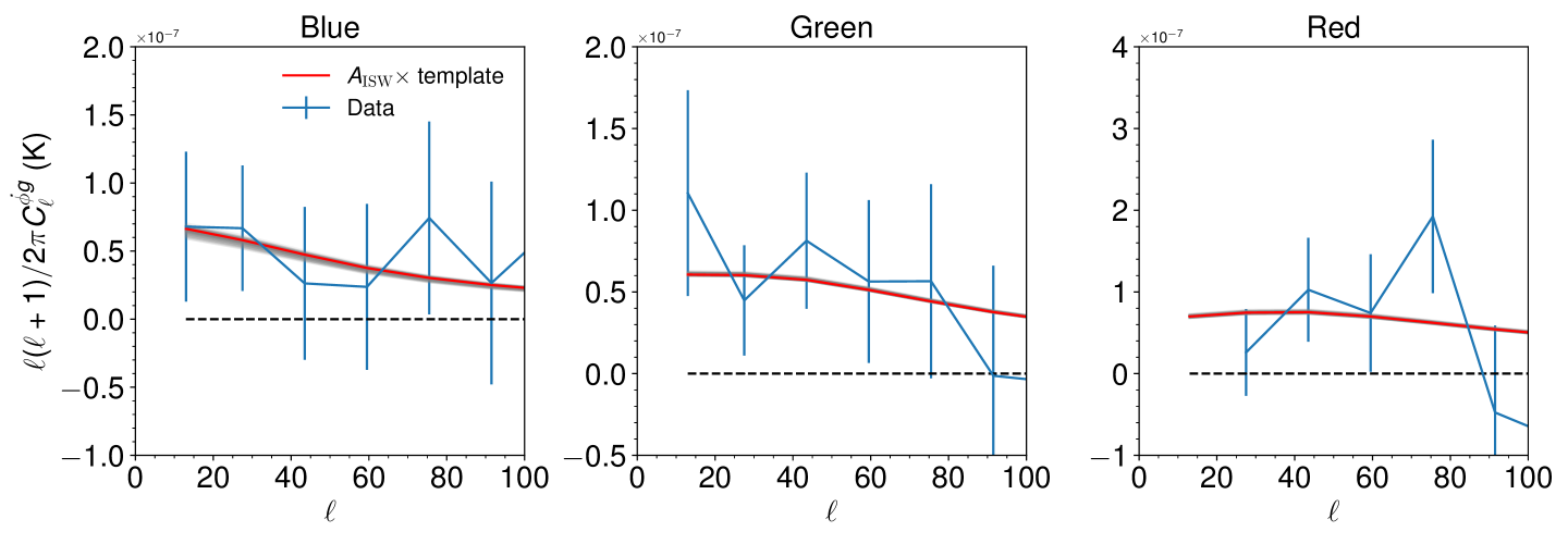
Figure 5: ISW data (blue) and prediction in the $\Lambda$CDM Planck cosmology, scaled by $A_{\rm ISW}$ (red) for the three unWISE samples. Errors are from the mock-based covariance in Fig. 4. The gray range around the theory curve is the uncertainty propgated from errors in $bdN/dz$.

Analysis	Blue $A_{\rm ISW}$	Green $A_{\rm ISW}$	Red $A_{\rm ISW}$
SMICA	$0.73\pm 0.34$	$1.00\pm 0.39$	$1.14\pm 0.52$
COMMANDER	$0.73\pm 0.34$	$0.99\pm 0.39$	$1.11\pm 0.52$
SEVEM	$0.76\pm 0.34$	$1.01\pm 0.39$	$1.15\pm 0.52$
NILC	$0.74\pm 0.34$	$1.00\pm 0.39$	$1.13\pm 0.52$
SMICA-NoSZ	$0.83\pm 0.34$	$1.07\pm 0.39$	$1.17\pm 0.52$
SEVEM 70 GHz	$0.66\pm 0.34$	$0.91\pm 0.39$	$1.12\pm 0.52$
SEVEM 100 GHz	$0.75\pm 0.34$	$0.97\pm 0.39$	$1.10\pm 0.52$
SEVEM 143 GHz	$0.76\pm 0.34$	$1.00\pm 0.39$	$1.14\pm 0.52$
SEVEM 217 GHz	$0.87\pm 0.34$	$1.04\pm 0.39$	$1.13\pm 0.52$
$m=0$ included	$0.69\pm 0.34$	$0.88\pm 0.39$	$1.03\pm 0.52$
Weighted galaxy field	$0.73\pm 0.34$	$0.98\pm 0.39$	$1.12\pm 0.52$

Table 2: $A_{\rm ISW}$ for the three unWISE samples for a variety of different systematics tests: changing the method used to construct the CMB temperature maps; including the $m=0$ mode; and applying weights to the galaxy field. The default analysis is shown on the top line with gray highlighting.

In Table 2, we perform a variety of systematics checks. We replace the default SMICA map with several other CMB temperature maps [93], and do not find that using any of these maps lead to a significant shift in $A_{\rm ISW}$. We also show that the results are not significantly affected by applying weights to the galaxy field or including the $m=0$ mode.

The uncertainty in $bdN/dz$ creates a systematic uncertainty in the theoretical prediction. We compute $A_{\rm ISW}$ using theoretical templates generated from each of the 100 samples of $bdN/dz$, with the bias taken from the corresponding fit of $C_{\ell}^{\kappa g}$ to that sample’s redshift distribution. We find uncertainties on $A_{\rm ISW}$ of 0.025, 0.0106, and 0.0180 for blue, green, and red, respectively. These systematic uncertainties are much smaller than the statistical errors on $A_{\rm ISW}$.

As Table 1 shows, the statistical uncertainties on $b^{\rm eff}$ are small (of order $1-2\%$) and thus contribute a negligible theoretical uncertainty compared to the large statistical errors on $A_{\rm ISW}$. Furthermore, the systematic uncertainties from nonlinear biasing are similar to the statistical uncertainties: if we restrict to $\ell<300$ (instead of the fiducial $\ell<1000$) we find $b^{\rm eff}=1.54$, 2.27 and 3.16 for the three samples, versus $b^{\rm eff}=1.50$, 2.23 and 3.19 if we use all data with $\ell<1000$. In Ref. [73], we also study other systematic errors on the redshift distribution and find them to be generally smaller than the errors from uncertain $dN/dz$. Therefore, we expect them to make a negligible contribution the ISW errorbars.

5.2 Comparison to dynamical dark energy

“Freezing” and “tracking” type behavior in the dark energy equation of state, $w$ (corresponding to $w=-1$ at late times and $w=0$ at early times, respectively), may be generic features of single scalar field theories [102, 51]. Since these models cause dark energy to act like matter at early times, increasing its energy density, they modify the ISW signal. Our measurement is particularly sensitive to these models if the transition from freezing to tracking occurs at $z\sim 1$ where the galaxy kernels peak.

As a specific example, we consider the Mocker model of Ref. [52, 103], which is a phenomenological description imitating the behavior of quintessence models. The Mocker model is defined by

$$\frac{dw}{d\log{a}}=Cw(1+w)$$ (5.1)

yielding the following equation of state, with free parameters $C$ and $w_{0}$

$$w(a)=-1+\left[1-\frac{w_{0}}{1+w_{0}}a^{C}\right]^{-1}$$ (5.2)

$w_{0}$ sets the $z=0$ equation of state, well constrained to be close to $-1$ by supernovae and BAO. $C$ controls the transition to a matter-like equation of state, with larger values of $C$ yielding a transition at lower redshift. The cosmological constant is recovered by $w_{0}=-1$. Observational constraints on this model have been considered in Ref. [44, 104, 51].

We consider constraints on the Mocker parameters from the ISW measurement in Fig. 6. We impose a flat prior on $C$ between 0 and $\infty$ and on $w_{0}$ between $-1$ and 0. We fix the other cosmological parameters to a flat cosmology with parameters identical to the ones used in the previous section: $\Omega_{m}h^{2}=0.1417$, $\theta_{\rm MC}=0.0104$, $\Omega_{b}h^{2}=0.0224$, $n_{s}=0.9665$, $\sigma_{8}=0.8102$, and one massive neutrino at 0.06 eV. We choose this parameterization as it is best constrained by the Planck primary CMB observations on smaller scales than the ones considered here. We use CAMBSources to compute $C_{\ell}^{Tg}$ in the Mocker model, using the DarkEnergyPPF class [105] to allow for an arbitrary $w(a)$.

The shape of the ISW posterior is determined by the fact that all models at $w_{0}=-1$ are equivalent, regardless of $C$; hence the posterior expands as $w_{0}$ approaches $-1$ and models with different $C$ become increasingly similar. The long non-zero tail in $C$ corresponds to models in which the transition from dark energy to matter occurs at very low redshift, where the ISW measurement is less sensitive due to the drop in the galaxy redshift distribution at $z<0.5$. ISW measurements from lower-redshift samples, or other measurements of the expansion history, can rule out these models with large $C$. For instance, the combination of unWISE ISW and Type Ia supernovae from Pantheon [106] can improve constraints on the Mocker models from Pantheon alone. If we also include BAO measurements, the constraints on Mocker models from the expansion history further improve the constraints.

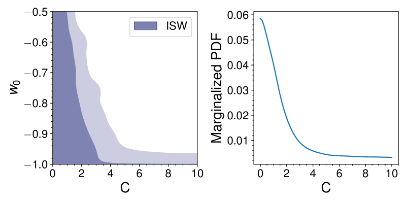
Figure 6: Left panel: one and two $\sigma$ constraints on mocker parameters $C$ and $w_{0}$ from unWISE ISW alone. The $w=-1$ axis corresponds to $\Lambda$CDM. Right panel: marginalized constraints on $C$ from unWISE ISW. Marginalized constraints on $w_{0}$ are much weaker than evidence from geometric probes that the Universe is dark energy dominated at low redshift. The ISW measurement provides more information on the evolution of the dark energy component through the parameter $C$.

In Fig. 7, we show constraints from ISW and expansion history measurements. We use the Pantheon compilation of Type Ia supernovae [106] and BAO from SDSS I-III (including Ly$\alpha$ forest auto-correlation and quasar cross-correlation) and 6dF [107, 108, 109]. Note that BAO and supernovae are uncalibrated standard rulers and candles; i.e. BAO constrains the ratio of the comoving distance to the sound horizon (and thus does not depend on knowing the absolute value of the sound horizon). The ISW measurement improves the constraint from supernovae alone, and when adding BAO, the constraints further tighten significantly. Our constraints improve upon those presented in [44, 104]; we find similar constraints on $C$ (marginalized 95% upper limit of $3.99$) and considerably improve the constraint on $w_{0}$ (marginalized 95% upper limit of $-0.97$). These represent the tightest constraint on the Mocker model to date, and constrain the dark energy density to be within $\sim 10\%$ of a cosmological constant (95% upper limit) at $z=2$ in these models.

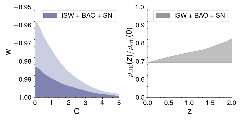
Figure 7: Left panel: constraints on mocker parameters $C$ and $w_{0}$ from ISW and from type Ia supernovae plus BAO. The $x$ axis corresponds to $\Lambda$CDM. Right panel: corresponding 95% upper limit on the dark energy density as a function of redshift, in the Mocker model.

6 Conclusions

Using Planck CMB temperature maps and unWISE galaxy maps over 60% of the sky, we detect the integrated Sachs-Wolfe correlation between galaxy density and CMB temperature at 3.2$\sigma$. We use three galaxy samples out to $z\sim 2$, and find $A_{\rm ISW}=0.73\pm 0.34$ in the $z\sim 0.5$ “blue” sample, $A_{\rm ISW}=1.00\pm 0.39$ in the $z\sim 1.0$ “green” sample, and $A_{\rm ISW}=1.14\pm 0.52$ in the $z\sim 1.5$ “red” sample. We find that this detection is robust to a number of changes in the analysis choices, suggesting it is not significantly affected by systematics. We also use this measurement to constrain a toy phenomenological model of freezing quintessence, the Mocker model. We find that the ISW measurement improves constraints on the Mocker model compared to type Ia supernovae, and adding BAO constraints we can obtain the tightest constraints. We provide updated constraints on the Mocker model with the latest BAO and supernovae datasets, constraining the dark energy density to within 10% at $z<2$.

We apply a number of tests to ensure the robustness of the ISW measurement. First, we include the lensing magnification-$\dot{\Phi}$ term in our theoretical modelling. This term is substantial for the green and red samples, 15-20% of the $g\dot{\Phi}$ term. Second, we remove $m=0$ modes (in a Galactic coordinate system) as these are most likely to be contaminated by systematics in the galaxy and ISW maps. We test and validate our pipeline on Gaussian mocks, and confirm the accuracy of the bandpower window function required to generate the binned theory power spectrum. Third, we conduct a variety of systematics tests, changing the CMB temperature map used, the minimum $\ell$ used, and applying weights to the galaxy field, as summarized in Table 2. Finally we measure the covariance of the ISW signal by cross-correlating the galaxy maps with 300 end-to-end Planck simulations with fully realistic noise.

This measurement represents a direct detection of the effects of dark energy, consistent with the best-fit $\Lambda$CDM cosmology from Planck with no statistically significant evidence for evolution in the dark energy density. Our results are quite consistent with previous ISW cross-correlation results [42, 38, 39] and inconsistent with the higher ISW amplitude reported using stacking around superclusters or supervoids [48, 49]. Overall, these results support the consensus flat $\Lambda$CDM cosmology and improve constraints on the dark energy density at $z\sim 1-2$ by 30-40%. While the ISW measurement is not as statistically significant as distance measurements supporting dark energy (i.e. type Ia supernovae and BAO), it complements them by constraining the time evolution of dark energy, and offering a purely gravitational rather than expansion-based constraint.

Appendix A Validating the bandpower window functions

Due to the effects of mode-coupling, the binned theory power spectrum is not identical to the mean of the theory power spectrum across each bin. Instead, the binned power spectrum in bin $b$ is the product of the bandpower window matrix $W$ and the unbinned power spectrum $C_{\ell}$

$$C_{b}=\sum_{\ell}W_{b\ell}C_{\ell}$$ (A.1)

The bandpower window matrix is the product of the mode-coupling matrix $M_{\ell\ell^{\prime}}$ and the binned mode-coupling matrix $\mathcal{M}_{bb^{\prime}}$ in Equations. 4.2 and 4.3

$$W_{b\ell}=\sum_{b^{\prime}}\mathcal{M}^{-1}_{bb^{\prime}}\sum_{\ell^{\prime}\in b^{\prime}}M_{\ell\ell^{\prime}}$$ (A.2)

The right panel of Fig. 8 shows the bandpower window matrix for the first five bins, and the unbinned theory spectra on the right axis. The left panel of Fig. 8 measures this effect empirically, by running the measurement pipeline on 100 Gaussian simulations and plotting the ratio between the binned bandpowers (averaged over simulations) and the mean of $C\textbf{}_{\ell}$ within each bin. The measurement in simulations is fully consistent with the expectation from the bandpower window matrix; the apparent large discrepancy in the lowest $\ell$ bin is not statistically significant and entirely due to cosmic variance in the bin. The dip at $\ell=35$ is expected because the theory power spectra peak around $\ell=35$; thus the tails of the bandpower window function both decrease the binned power spectrum. At higher $\ell$, the two tails partially cancel, but because the spectrum is a declining function of $\ell$, the binned power spectrum is slightly below the mean of the unbinned power spectrum.

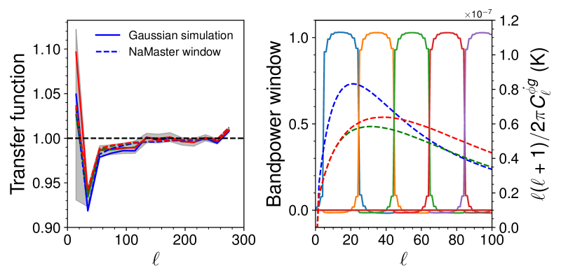
Figure 8: Left: Mask deconvolution transfer function for $C_{\ell}^{Tg}$ measurement, i.e. the ratio between the mean of the unbinned $C_{\ell}^{Tg}$, and the output binned power spectrum after masking, pseudo-$C_{\ell}$ estimation, and mask deconvolution. The transfer function was computed by averaging over 100 Gaussian simulations. $C_{\ell}^{gg}$ in the simulation is a smoothed version of the measured $C_{\ell}^{gg}$, including an uptick at low $\ell$ above a theory curve fit to $C_{\ell}^{gg}$ at $\ell>100$, presumably due to uncorrected systematics. The transfer function from the Gaussian simulation is compared to the product of the bandpower window matrix and the unbinned power spectrum (dashed line). The NaMaster window is perfectly consistent with the Gaussian simulations within the error on the simulations (gray band). Right: The bandpower window functions (left axis) and the unbinned theory spectra (right axis). The product of these two quantities, divided by the mean of the unbinned spectrum in each bin, gives the dashed line in the left panel.

References

- [1] R. K. Sachs and A. M. Wolfe, Perturbations of a Cosmological Model and Angular Variations of the Microwave Background, ApJ 147 (1967) 73.
- [2] M. J. Rees and D. W. Sciama, Large-scale Density Inhomogeneities in the Universe, Nature 217 (1968) 511.
- [3] M. White and W. Hu, The Sachs-Wolfe effect., A&A 321 (1997) 8 [astro-ph/9609105].
- [4] A. G. Riess, A. V. Filippenko, P. Challis, A. Clocchiatti, A. Diercks, P. M. Garnavich et al., Observational Evidence from Supernovae for an Accelerating Universe and a Cosmological Constant, AJ 116 (1998) 1009 [astro-ph/9805201].
- [5] S. Perlmutter, G. Aldering, G. Goldhaber, R. A. Knop, P. Nugent, P. G. Castro et al., Measurements of and from 42 High-Redshift Supernovae, ApJ 517 (1999) 565 [astro-ph/9812133].
- [6] A. G. Riess, L.-G. Strolger, J. Tonry, S. Casertano, H. C. Ferguson, B. Mobasher et al., Type Ia Supernova Discoveries at z > 1 from the Hubble Space Telescope: Evidence for Past Deceleration and Constraints on Dark Energy Evolution, ApJ 607 (2004) 665 [astro-ph/0402512].
- [7] R. G. Crittenden and N. Turok, Looking for a Cosmological Constant with the Rees-Sciama Effect, Phys. Rev. Lett. 76 (1996) 575 [astro-ph/9510072].
- [8] W. Hu, Dark synergy: Gravitational lensing and the CMB, PRD 65 (2002) 023003 [astro-ph/0108090].
- [9] J. Renk, M. Zumalacárregui, F. Montanari and A. Barreira, Galileon gravity in light of ISW, CMB, BAO and H0 data, JCAP 2017 (2017) 020 [1707.02263].
- [10] M. Kamionkowski, Matter-microwave correlations in an open universe, PRD 54 (1996) 4169 [astro-ph/9602150].
- [11] A. Cooray, Nonlinear integrated Sachs-Wolfe effect, PRD 65 (2002) 083518 [astro-ph/0109162].
- [12] M. Birkinshaw and S. F. Gull, A test for transverse motions of clusters of galaxies, Nature 302 (1983) 315.
- [13] A. Stebbins, Measuring velocites using the CMB \& LSS, New Astron. Rev. 50 (2006) 918.
- [14] S. C. Hotinli, J. Meyers, N. Dalal, A. H. Jaffe, M. C. Johnson, J. B. Mertens et al., Transverse Velocities with the Moving Lens Effect, Phys. Rev. Lett. 123 (2019) 061301 [1812.03167].
- [15] S. C. Hotinli, M. C. Johnson and J. Meyers, Optimal filters for the moving lens effect, Phys. Rev. D 103 (2021) 043536 [2006.03060].
- [16] S. C. Hotinli, K. M. Smith, M. S. Madhavacheril and M. Kamionkowski, Cosmology with the moving lens effect, 2108.02207.
- [17] S. Yasini, N. Mirzatuny and E. Pierpaoli, Pairwise Transverse Velocity Measurement with the Rees–Sciama Effect, Astrophys. J. Lett. 873 (2019) L23 [1812.04241].
- [18] R. Hagala, C. Llinares and D. F. Mota, The slingshot effect as a probe of transverse motions of galaxies, Astron. Astrophys. 628 (2019) A30 [1907.01429].
- [19] S. Boughn and R. Crittenden, A correlation between the cosmic microwave background and large-scale structure in the Universe, Nature 427 (2004) 45 [astro-ph/0305001].
- [20] R. Scranton, A. J. Connolly, R. C. Nichol, A. Stebbins, I. Szapudi, D. J. Eisenstein et al., Physical Evidence for Dark Energy, arXiv e-prints (2003) astro [astro-ph/0307335].
- [21] P. Fosalba, E. Gaztañaga and F. J. Castand er, Detection of the Integrated Sachs-Wolfe and Sunyaev-Zeldovich Effects from the Cosmic Microwave Background-Galaxy Correlation, ApJL 597 (2003) L89 [astro-ph/0307249].
- [22] M. R. Nolta, E. L. Wright, L. Page, C. L. Bennett, M. Halpern, G. Hinshaw et al., First Year Wilkinson Microwave Anisotropy Probe Observations: Dark Energy Induced Correlation with Radio Sources, ApJ 608 (2004) 10 [astro-ph/0305097].
- [23] P.-S. Corasaniti, T. Giannantonio and A. Melchiorri, Constraining dark energy with cross-correlated CMB and large scale structure data, PRD 71 (2005) 123521 [astro-ph/0504115].
- [24] N. Padmanabhan, C. M. Hirata, U. Seljak, D. J. Schlegel, J. Brinkmann and D. P. Schneider, Correlating the CMB with luminous red galaxies: The integrated Sachs-Wolfe effect, PRD 72 (2005) 043525 [astro-ph/0410360].
- [25] P. Vielva, E. Martínez-González and M. Tucci, Cross-correlation of the cosmic microwave background and radio galaxies in real, harmonic and wavelet spaces: detection of the integrated Sachs-Wolfe effect and dark energy constraints, MNRAS 365 (2006) 891 [astro-ph/0408252].
- [26] T. Giannantonio, R. G. Crittenden, R. C. Nichol, R. Scranton, G. T. Richards, A. D. Myers et al., High redshift detection of the integrated Sachs-Wolfe effect, PRD 74 (2006) 063520 [astro-ph/0607572].
- [27] A. Cabré, E. Gaztañaga, M. Manera, P. Fosalba and F. Castander, Cross-correlation of Wilkinson Microwave Anisotropy Probe third-year data and the Sloan Digital Sky Survey DR4 galaxy survey: new evidence for dark energy, MNRAS 372 (2006) L23 [astro-ph/0603690].
- [28] A. Rassat, K. Land, O. Lahav and F. B. Abdalla, Cross-correlation of 2MASS and WMAP 3: implications for the integrated Sachs-Wolfe effect, MNRAS 377 (2007) 1085 [astro-ph/0610911].
- [29] J. D. McEwen, P. Vielva, M. P. Hobson, E. Martínez-González and A. N. Lasenby, Detection of the integrated Sachs-Wolfe effect and corresponding dark energy constraints made with directional spherical wavelets, MNRAS 376 (2007) 1211 [astro-ph/0605122].
- [30] S. Ho, C. Hirata, N. Padmanabhan, U. Seljak and N. Bahcall, Correlation of CMB with large-scale structure. I. Integrated Sachs-Wolfe tomography and cosmological implications, PRD 78 (2008) 043519 [0801.0642].
- [31] T. Giannantonio, R. Crittenden, R. Nichol and A. J. Ross, The significance of the integrated Sachs-Wolfe effect revisited, MNRAS 426 (2012) 2581 [1209.2125].
- [32] T. Goto, I. Szapudi and B. R. Granett, Cross-correlation of WISE galaxies with the cosmic microwave background, MNRAS 422 (2012) L77 [1202.5306].
- [33] C. Hernández-Monteagudo, A. J. Ross, A. Cuesta, R. Génova-Santos, J.-Q. Xia, F. Prada et al., The SDSS-III Baryonic Oscillation Spectroscopic Survey: constraints on the integrated Sachs-Wolfe effect, MNRAS 438 (2014) 1724 [1303.4302].
- [34] S. Ferraro, B. D. Sherwin and D. N. Spergel, WISE measurement of the integrated Sachs-Wolfe effect, PRD 91 (2015) 083533 [1401.1193].
- [35] E. Moura-Santos, F. C. Carvalho, M. Penna-Lima, C. P. Novaes and C. A. Wuensche, A Bayesian Estimate of the CMB-Large-scale Structure Cross-correlation, ApJ 826 (2016) 121 [1512.00641].
- [36] A. J. Shajib and E. L. Wright, Measurement of the Integrated Sachs-Wolfe Effect Using the AllWISE Data Release, ApJ 827 (2016) 116 [1604.03939].
- [37] Planck Collaboration, P. A. R. Ade, N. Aghanim, C. Armitage-Caplan, M. Arnaud, M. Ashdown et al., Planck 2013 results. XIX. The integrated Sachs-Wolfe effect, A&A 571 (2014) A19 [1303.5079].
- [38] Planck Collaboration, P. A. R. Ade, N. Aghanim, M. Arnaud, M. Ashdown, J. Aumont et al., Planck 2015 results. XXI. The integrated Sachs-Wolfe effect, A&A 594 (2016) A21 [1502.01595].
- [39] B. Stölzner, A. Cuoco, J. Lesgourgues and M. Bilicki, Updated tomographic analysis of the integrated Sachs-Wolfe effect and implications for dark energy, PRD 97 (2018) 063506 [1710.03238].
- [40] B. Ansarinejad, R. Mackenzie, T. Shanks and N. Metcalfe, Cross-correlating Planck with VST ATLAS LRGs: a new test for the ISW effect in the Southern hemisphere, MNRAS 493 (2020) 4830 [1909.11095].
- [41] Q. Hang, S. Alam, J. A. Peacock and Y.-C. Cai, Galaxy clustering in the DESI Legacy Survey and its imprint on the CMB, MNRAS 501 (2021) 1481 [2010.00466].
- [42] T. Giannantonio, R. Scranton, R. G. Crittenden, R. C. Nichol, S. P. Boughn, A. D. Myers et al., Combined analysis of the integrated Sachs-Wolfe effect and cosmological implications, PRD 77 (2008) 123520 [0801.4380].
- [43] D. Pietrobon, A. Balbi and D. Marinucci, Integrated Sachs-Wolfe effect from the cross correlation of WMAP 3year and the NRAO VLA sky survey data: New results and constraints on dark energy, PRD 74 (2006) 043524 [astro-ph/0606475].
- [44] J.-Q. Xia, M. Viel, C. Baccigalupi and S. Matarrese, The high redshift Integrated Sachs-Wolfe effect, JCAP 2009 (2009) 003 [0907.4753].
- [45] G.-B. Zhao, T. Giannantonio, L. Pogosian, A. Silvestri, D. J. Bacon, K. Koyama et al., Probing modifications of general relativity using current cosmological observations, PRD 81 (2010) 103510 [1003.0001].
- [46] H. Li and J.-Q. Xia, Constraints on dark energy parameters from correlations of CMB with LSS, JCAP 2010 (2010) 026 [1004.2774].
- [47] E. F. Schlafly, A. M. Meisner and G. M. Green, The unWISE Catalog: Two Billion Infrared Sources from Five Years of WISE Imaging, The Astrophysical Journal Supplement Series 240 (2019) 30 [1901.03337].
- [48] B. R. Granett, M. C. Neyrinck and I. Szapudi, An Imprint of Superstructures on the Microwave Background due to the Integrated Sachs-Wolfe Effect, ApJL 683 (2008) L99 [0805.3695].
- [49] A. Kovács, C. Sánchez, J. García-Bellido, J. Elvin-Poole, N. Hamaus, V. Miranda et al., More out of less: an excess integrated Sachs-Wolfe signal from supervoids mapped out by the Dark Energy Survey, MNRAS 484 (2019) 5267 [1811.07812].
- [50] A. Kovács, R. Beck, A. Smith, G. Rácz, I. Csabai and I. Szapudi, Evidence for a high-z ISW signal from supervoids in the distribution of eBOSS quasars, arXiv e-prints (2021) arXiv:2107.13038 [2107.13038].
- [51] P. Bull, M. White and A. Slosar, Searching for dark energy in the matter-dominated era, MNRAS 505 (2021) 2285 [2007.02865].
- [52] E. V. Linder, Paths of quintessence, PRD 73 (2006) 063010 [astro-ph/0601052].
- [53] E. V. Linder, Dark Energy in the Dark Ages, Astropart. Phys. 26 (2006) 16 [astro-ph/0603584].
- [54] V. Poulin, T. L. Smith, T. Karwal and M. Kamionkowski, Early Dark Energy can Resolve the Hubble Tension, Phys. Rev. Lett. 122 (2019) 221301 [1811.04083].
- [55] P. Agrawal, F.-Y. Cyr-Racine, D. Pinner and L. Randall, Rock ’n’ Roll Solutions to the Hubble Tension, arXiv e-prints (2019) arXiv:1904.01016 [1904.01016].
- [56] M.-X. Lin, G. Benevento, W. Hu and M. Raveri, Acoustic dark energy: Potential conversion of the Hubble tension, PRD 100 (2019) 063542 [1905.12618].
- [57] T. L. Smith, V. Poulin and M. A. Amin, Oscillating scalar fields and the Hubble tension: A resolution with novel signatures, PRD 101 (2020) 063523 [1908.06995].
- [58] J. C. Hill, E. Calabrese, S. Aiola, N. Battaglia, B. Bolliet, S. K. Choi et al., The Atacama Cosmology Telescope: Constraints on Pre-Recombination Early Dark Energy, arXiv e-prints (2021) arXiv:2109.04451 [2109.04451].
- [59] S. Vagnozzi, Consistency tests of CDM from the early integrated Sachs-Wolfe effect: Implications for early-time new physics and the Hubble tension, PRD 104 (2021) 063524 [2105.10425].
- [60] Y.-C. Cai, S. Cole, A. Jenkins and C. S. Frenk, Full-sky map of the ISW and Rees-Sciama effect from Gpc simulations, MNRAS 407 (2010) 201 [1003.0974].
- [61] A. J. Mead, J. A. Peacock, C. Heymans, S. Joudaki and A. F. Heavens, An accurate halo model for fitting non-linear cosmological power spectra and baryonic feedback models, MNRAS 454 (2015) 1958 [1505.07833].
- [62] A. Challinor and A. Lewis, The linear power spectrum of observed source number counts, PRD 84 (2011) 043516 [1105.5292].
- [63] A. Lewis, A. Challinor and A. Lasenby, Efficient computation of CMB anisotropies in closed FRW models, ApJ 538 (2000) 473 [astro-ph/9911177].
- [64] C. Howlett, A. Lewis, A. Hall and A. Challinor, CMB power spectrum parameter degeneracies in the era of precision cosmology, JCAP 1204 (2012) 027 [1201.3654].
- [65] E. L. Wright, P. R. M. Eisenhardt, A. K. Mainzer, M. E. Ressler, R. M. Cutri, T. Jarrett et al., The Wide-field Infrared Survey Explorer (WISE): Mission Description and Initial On-orbit Performance, AJ 140 (2010) 1868 [1008.0031].
- [66] A. Mainzer, J. Bauer, T. Grav, J. Masiero, R. M. Cutri, J. Dailey et al., Preliminary Results from NEOWISE: An Enhancement to the Wide-field Infrared Survey Explorer for Solar System Science, ApJ 731 (2011) 53 [1102.1996].
- [67] A. Mainzer, J. Bauer, R. M. Cutri, T. Grav, J. Masiero, R. Beck et al., Initial Performance of the NEOWISE Reactivation Mission, ApJ 792 (2014) 30 [1406.6025].
- [68] A. M. Meisner, D. Lang and D. J. Schlegel, Full-depth Coadds of the WISE and First-year NEOWISE-reactivation Images, AJ 153 (2017) 38 [1603.05664].
- [69] A. M. Meisner, D. Lang and D. J. Schlegel, Deep Full-sky Coadds from Three Years of WISE and NEOWISE Observations, AJ 154 (2017) 161 [1705.06746].
- [70] A. M. Meisner, D. Lang and D. J. Schlegel, Another unWISE Update: The Deepest Ever Full-sky Maps at 3-5 m, Research Notes of the American Astronomical Society 2 (2018) 1 [1801.03566].
- [71] A. M. Meisner, D. Lang, E. F. Schlafly and D. J. Schlegel, unWISE Coadds: The Five-year Data Set, Publ. Astron. Soc. Pac. 131 (2019) 124504 [1909.05444].
- [72] C. Laigle, C. Pichon, S. Codis, Y. Dubois, D. Le Borgne, D. Pogosyan et al., Swirling around filaments: are large-scale structure vortices spinning up dark haloes?, MNRAS 446 (2015) 2744.
- [73] A. Krolewski, S. Ferraro, E. F. Schlafly and M. White, unWISE tomography of Planck CMB lensing, arXiv e-prints (2019) arXiv:1909.07412 [1909.07412].
- [74] A. Krolewski, S. Ferraro and M. White, Cosmological constraints from unWISE and Planck CMB lensing tomography, arXiv e-prints (2021) arXiv:2105.03421 [2105.03421].
- [75] C. Laigle, H. J. McCracken, O. Ilbert, B. C. Hsieh, I. Davidzon, P. Capak et al., The COSMOS2015 Catalog: Exploring the 1 z 6 Universe with Half a Million Galaxies, ApJS 224 (2016) 24 [1604.02350].
- [76] Gaia Collaboration, A. G. A. Brown, A. Vallenari, T. Prusti, J. H. J. de Bruijne, C. Babusiaux et al., Gaia Data Release 2. Summary of the contents and survey properties, A&A 616 (2018) A1 [1804.09365].
- [77] Planck Collaboration, N. Aghanim, Y. Akrami, M. Ashdown, J. Aumont, C. Baccigalupi et al., Planck 2018 results. VIII. Gravitational lensing, ArXiv e-prints (2018) [1807.06210].
- [78] A. J. Ross, W. J. Percival, A. G. Sánchez, L. Samushia, S. Ho, E. Kazin et al., The clustering of galaxies in the SDSS-III Baryon Oscillation Spectroscopic Survey: analysis of potential systematics, MNRAS 424 (2012) 564 [1203.6499].
- [79] A. J. Ross, F. Beutler, C.-H. Chuang, M. Pellejero-Ibanez, H.-J. Seo, M. Vargas-Magaña et al., The clustering of galaxies in the completed SDSS-III Baryon Oscillation Spectroscopic Survey: observational systematics and baryon acoustic oscillations in the correlation function, MNRAS 464 (2017) 1168 [1607.03145].
- [80] M. Ata, F. Baumgarten, J. Bautista, F. Beutler, D. Bizyaev, M. R. Blanton et al., The clustering of the SDSS-IV extended Baryon Oscillation Spectroscopic Survey DR14 quasar sample: first measurement of baryon acoustic oscillations between redshift 0.8 and 2.2, MNRAS 473 (2018) 4773 [1705.06373].
- [81] J. E. Bautista, M. Vargas-Magaña, K. S. Dawson, W. J. Percival, J. Brinkmann, J. Brownstein et al., The SDSS-IV Extended Baryon Oscillation Spectroscopic Survey: Baryon Acoustic Oscillations at Redshift of 0.72 with the DR14 Luminous Red Galaxy Sample, ApJ 863 (2018) 110 [1712.08064].
- [82] J. Elvin-Poole, M. Crocce, A. J. Ross, T. Giannantonio, E. Rozo, E. S. Rykoff et al., Dark Energy Survey year 1 results: Galaxy clustering for combined probes, PRD 98 (2018) 042006 [1708.01536].
- [83] A. J. Ross, J. Bautista, R. Tojeiro, S. Alam, S. Bailey, E. Burtin et al., The Completed SDSS-IV extended Baryon Oscillation Spectroscopic Survey: Large-scale structure catalogues for cosmological analysis, MNRAS 498 (2020) 2354 [2007.09000].
- [84] M. Rodríguez-Monroy, N. Weaverdyck, J. Elvin-Poole, M. Crocce, A. Carnero Rosell, F. Andrade-Oliveira et al., Dark Energy Survey Year 3 Results: Galaxy clustering and systematics treatment for lens galaxy samples, arXiv e-prints (2021) arXiv:2105.13540 [2105.13540].
- [85] K. M. Górski, E. Hivon, A. J. Banday, B. D. Wand elt, F. K. Hansen, M. Reinecke et al., HEALPix: A Framework for High-Resolution Discretization and Fast Analysis of Data Distributed on the Sphere, ApJ 622 (2005) 759 [astro-ph/0409513].
- [86] D. J. Schlegel, D. P. Finkbeiner and M. Davis, Maps of Dust Infrared Emission for Use in Estimation of Reddening and Cosmic Microwave Background Radiation Foregrounds, ApJ 500 (1998) 525 [astro-ph/9710327].
- [87] HI4PI Collaboration, N. Ben Bekhti, L. Flöer, R. Keller, J. Kerp, D. Lenz et al., HI4PI: A full-sky H I survey based on EBHIS and GASS, A&A 594 (2016) A116 [1610.06175].
- [88] T. Kelsall, J. L. Weiland, B. A. Franz, W. T. Reach, R. G. Arendt, E. Dwek et al., The COBE Diffuse Infrared Background Experiment Search for the Cosmic Infrared Background. II. Model of the Interplanetary Dust Cloud, ApJ 508 (1998) 44 [astro-ph/9806250].
- [89] J. A. Newman, Calibrating Redshift Distributions beyond Spectroscopic Limits with Cross-Correlations, ApJ 684 (2008) 88 [0805.1409].
- [90] M. McQuinn and M. White, On using angular cross-correlations to determine source redshift distributions, MNRAS 433 (2013) 2857 [1302.0857].
- [91] B. Ménard, R. Scranton, S. Schmidt, C. Morrison, D. Jeong, T. Budavari et al., Clustering-based redshift estimation: method and application to data, arXiv e-prints (2013) [1303.4722].
- [92] S. Alam, M. Aubert, S. Avila, C. Balland, J. E. Bautista, M. A. Bershady et al., Completed SDSS-IV extended Baryon Oscillation Spectroscopic Survey: Cosmological implications from two decades of spectroscopic surveys at the Apache Point Observatory, PRD 103 (2021) 083533 [2007.08991].
- [93] Planck Collaboration, Y. Akrami, M. Ashdown, J. Aumont, C. Baccigalupi, M. Ballardini et al., Planck 2018 results. IV. Diffuse component separation, arXiv e-prints (2018) arXiv:1807.06208 [1807.06208].
- [94] Planck Collaboration, Y. Akrami, F. Argüeso, M. Ashdown, J. Aumont, C. Baccigalupi et al., Planck 2018 results. II. Low Frequency Instrument data processing, arXiv e-prints (2018) arXiv:1807.06206 [1807.06206].
- [95] Planck Collaboration, N. Aghanim, Y. Akrami, M. Ashdown, J. Aumont, C. Baccigalupi et al., Planck 2018 results. III. High Frequency Instrument data processing and frequency maps, arXiv e-prints (2018) arXiv:1807.06207 [1807.06207].
- [96] E. Hivon, K. M. Górski, C. B. Netterfield, B. P. Crill, S. Prunet and F. Hansen, MASTER of the Cosmic Microwave Background Anisotropy Power Spectrum: A Fast Method for Statistical Analysis of Large and Complex Cosmic Microwave Background Data Sets, ApJ 567 (2002) 2 [astro-ph/0105302].
- [97] D. Alonso, J. Sanchez and A. Slosar, A unified pseudo- framework, ArXiv e-prints (2018) [1809.09603].
- [98] J. Hartlap, P. Simon and P. Schneider, Why your model parameter confidences might be too optimistic. Unbiased estimation of the inverse covariance matrix, A&A 464 (2007) 399 [astro-ph/0608064].
- [99] L. Knox, Determination of inflationary observables by cosmic microwave background anisotropy experiments, PRD 52 (1995) 4307 [astro-ph/9504054].
- [100] G. Efstathiou, Myths and truths concerning estimation of power spectra, Mon. Not. Roy. Astron. Soc. 349 (2004) 603 [astro-ph/0307515].
- [101] N. Afshordi, Integrated Sachs-Wolfe effect in cross-correlation: The observer’s manual, PRD 70 (2004) 083536 [astro-ph/0401166].
- [102] M. Raveri, P. Bull, A. Silvestri and L. Pogosian, Priors on the effective dark energy equation of state in scalar-tensor theories, PRD 96 (2017) 083509 [1703.05297].
- [103] E. V. Linder, On oscillating dark energy, Astroparticle Physics 25 (2006) 167 [astro-ph/0511415].
- [104] J.-Q. Xia and M. Viel, Early dark energy at high redshifts: status and perspectives, JCAP 2009 (2009) 002 [0901.0605].
- [105] W. Fang, W. Hu and A. Lewis, Crossing the phantom divide with parametrized post-friedmann dark energy, Physical Review D 78 (2008) .
- [106] D. M. Scolnic, D. O. Jones, A. Rest, Y. C. Pan, R. Chornock, R. J. Foley et al., The Complete Light-curve Sample of Spectroscopically Confirmed SNe Ia from Pan-STARRS1 and Cosmological Constraints from the Combined Pantheon Sample, ApJ 859 (2018) 101 [1710.00845].
- [107] F. Beutler, C. Blake, M. Colless, D. H. Jones, L. Staveley-Smith, L. Campbell et al., The 6dF Galaxy Survey: baryon acoustic oscillations and the local Hubble constant, MNRAS 416 (2011) 3017 [1106.3366].
- [108] A. J. Ross, L. Samushia, C. Howlett, W. J. Percival, A. Burden and M. Manera, The clustering of the SDSS DR7 main Galaxy sample - I. A 4 per cent distance measure at z = 0.15, MNRAS 449 (2015) 835 [1409.3242].
- [109] S. Alam, M. Aubert, S. Avila, C. Balland, J. E. Bautista, M. A. Bershady et al., Completed SDSS-IV extended Baryon Oscillation Spectroscopic Survey: Cosmological implications from two decades of spectroscopic surveys at the Apache Point Observatory, PRD 103 (2021) 083533 [2007.08991].
- [110] J. Torrado and A. Lewis, Cobaya: Bayesian analysis in cosmology, Oct., 2019.
- [111] J. Torrado and A. Lewis, Cobaya: code for bayesian analysis of hierarchical physical models, Journal of Cosmology and Astroparticle Physics 2021 (2021) 057.
- [112] A. Lewis, Getdist: a python package for analysing monte carlo samples, 2019.