2 Sorbonne Universités, UPMC Univ Paris 6 et CNRS, UMR 7095, Institut d’Astrophysique de Paris, 98 bis bd Arago, 75014 Paris, France
3 Aix-Marseille Univ, CNRS, CNES, LAM, Marseille, France
4 Cosmic Dawn Center (DAWN), Niels Bohr Institute, University of Copenhagen, Vibenshuset, Lyngbyvej 2, DK-2100 Copenhagen, Denmark
5 Minnesota Institute for Astrophysics, University of Minnesota, 116 Church St SE, Minneapolis, MN 55455, USA
6 Cosmic Dawn Center (DAWN)
7 Niels Bohr Institute, University of Copenhagen, Jagtvej 128, 2200 Copenhagen, Denmark
8 Infrared Processing and Analysis Center, California Institute of Technology, Pasadena, CA 91125, USA
9 California institute of Technology, 1200 E California Blvd, Pasadena, CA 91125, USA
10 Physics and Astronomy Department, University of California, 900 University Ave., Riverside, CA 92521, USA
11 Institute for Astronomy, University of Hawaii, 2680 Woodlawn Drive, Honolulu, HI 96822, USA
12 INFN-Sezione di Roma, Piazzale Aldo Moro, 2 - c/o Dipartimento di Fisica, Edificio G. Marconi, I-00185 Roma, Italy
13 INAF-Osservatorio Astronomico di Roma, Via Frascati 33, I-00078 Monteporzio Catone, Italy
14 Jet Propulsion Laboratory, California Institute of Technology, 4800 Oak Grove Drive, Pasadena, CA, 91109, USA
15 Institute of Cosmology and Gravitation, University of Portsmouth, Portsmouth PO1 3FX, UK
16 INAF-Osservatorio di Astrofisica e Scienza dello Spazio di Bologna, Via Piero Gobetti 93/3, I-40129 Bologna, Italy
17 Max Planck Institute for Extraterrestrial Physics, Giessenbachstr. 1, D-85748 Garching, Germany
18 INAF-Osservatorio Astrofisico di Torino, Via Osservatorio 20, I-10025 Pino Torinese (TO), Italy
19 INFN-Sezione di Roma Tre, Via della Vasca Navale 84, I-00146, Roma, Italy
20 Department of Mathematics and Physics, Roma Tre University, Via della Vasca Navale 84, I-00146 Rome, Italy
21 Institut de Recherche en Astrophysique et Planétologie (IRAP), Université de Toulouse, CNRS, UPS, CNES, 14 Av. Edouard Belin, F-31400 Toulouse, France
22 INAF-Osservatorio Astronomico di Capodimonte, Via Moiariello 16, I-80131 Napoli, Italy
23 Centro de Astrofísica da Universidade do Porto, Rua das Estrelas, 4150-762 Porto, Portugal
24 Instituto de Astrofísica e Ciências do Espaço, Universidade do Porto, CAUP, Rua das Estrelas, PT4150-762 Porto, Portugal
25 INAF-IASF Milano, Via Alfonso Corti 12, I-20133 Milano, Italy
26 Port d’Informació Científica, Campus UAB, C. Albareda s/n, 08193 Bellaterra (Barcelona), Spain
27 Institut de Física d’Altes Energies (IFAE), The Barcelona Institute of Science and Technology, Campus UAB, 08193 Bellaterra (Barcelona), Spain
28 Institute of Space Sciences (ICE, CSIC), Campus UAB, Carrer de Can Magrans, s/n, 08193 Barcelona, Spain
29 Institut d’Estudis Espacials de Catalunya (IEEC), Carrer Gran Capitá 2-4, 08034 Barcelona, Spain
30 Department of Physics ”E. Pancini”, University Federico II, Via Cinthia 6, I-80126, Napoli, Italy
31 INFN section of Naples, Via Cinthia 6, I-80126, Napoli, Italy
32 Dipartimento di Fisica e Astronomia ”Augusto Righi” - Alma Mater Studiorum Universitá di Bologna, Viale Berti Pichat 6/2, I-40127 Bologna, Italy
33 INAF-Osservatorio Astrofisico di Arcetri, Largo E. Fermi 5, I-50125, Firenze, Italy
34 Institut national de physique nucléaire et de physique des particules, 3 rue Michel-Ange, 75794 Paris Cédex 16, France
35 Centre National d’Etudes Spatiales, Toulouse, France
36 Institute for Astronomy, University of Edinburgh, Royal Observatory, Blackford Hill, Edinburgh EH9 3HJ, UK
37 Jodrell Bank Centre for Astrophysics, School of Physics and Astronomy, University of Manchester, Oxford Road, Manchester M13 9PL, UK
38 European Space Agency/ESRIN, Largo Galileo Galilei 1, 00044 Frascati, Roma, Italy
39 ESAC/ESA, Camino Bajo del Castillo, s/n., Urb. Villafranca del Castillo, 28692 Villanueva de la Cañada, Madrid, Spain
40 Univ Lyon, Univ Claude Bernard Lyon 1, CNRS/IN2P3, IP2I Lyon, UMR 5822, F-69622, Villeurbanne, France
41 Mullard Space Science Laboratory, University College London, Holmbury St Mary, Dorking, Surrey RH5 6NT, UK
42 Departamento de Física, Faculdade de Ciências, Universidade de Lisboa, Edifício C8, Campo Grande, PT1749-016 Lisboa, Portugal
43 Instituto de Astrofísica e Ciências do Espaço, Faculdade de Ciências, Universidade de Lisboa, Campo Grande, PT-1749-016 Lisboa, Portugal
44 Department of Astronomy, University of Geneva, ch. dÉcogia 16, CH-1290 Versoix, Switzerland
45 Université Paris-Saclay, CNRS, Institut d’astrophysique spatiale, 91405, Orsay, France
46 Department of Physics, Oxford University, Keble Road, Oxford OX1 3RH, UK
47 INFN-Padova, Via Marzolo 8, I-35131 Padova, Italy
48 AIM, CEA, CNRS, Université Paris-Saclay, Université de Paris, F-91191 Gif-sur-Yvette, France
49 INAF-Osservatorio Astronomico di Trieste, Via G. B. Tiepolo 11, I-34131 Trieste, Italy
50 Istituto Nazionale di Astrofisica (INAF) - Osservatorio di Astrofisica e Scienza dello Spazio (OAS), Via Gobetti 93/3, I-40127 Bologna, Italy
51 Istituto Nazionale di Fisica Nucleare, Sezione di Bologna, Via Irnerio 46, I-40126 Bologna, Italy
52 INAF-Osservatorio Astronomico di Brera, Via Brera 28, I-20122 Milano, Italy
53 INAF-Osservatorio Astronomico di Padova, Via dell’Osservatorio 5, I-35122 Padova, Italy
54 Universitäts-Sternwarte München, Fakultät für Physik, Ludwig-Maximilians-Universität München, Scheinerstrasse 1, 81679 München, Germany
55 Institute of Theoretical Astrophysics, University of Oslo, P.O. Box 1029 Blindern, N-0315 Oslo, Norway
56 Leiden Observatory, Leiden University, Niels Bohrweg 2, 2333 CA Leiden, The Netherlands
57 von Hoerner & Sulger GmbH, SchloßPlatz 8, D-68723 Schwetzingen, Germany
58 Max-Planck-Institut für Astronomie, Königstuhl 17, D-69117 Heidelberg, Germany
59 Aix-Marseille Univ, CNRS/IN2P3, CPPM, Marseille, France
60 Université de Genève, Département de Physique Théorique and Centre for Astroparticle Physics, 24 quai Ernest-Ansermet, CH-1211 Genève 4, Switzerland
61 Department of Physics and Helsinki Institute of Physics, Gustaf Hällströmin katu 2, 00014 University of Helsinki, Finland
62 NOVA optical infrared instrumentation group at ASTRON, Oude Hoogeveensedijk 4, 7991PD, Dwingeloo, The Netherlands
63 Argelander-Institut für Astronomie, Universität Bonn, Auf dem Hügel 71, 53121 Bonn, Germany
64 Dipartimento di Fisica e Astronomia “Augusto Righi” - Alma Mater Studiorum Università di Bologna, via Piero Gobetti 93/2, I-40129 Bologna, Italy
65 INFN-Sezione di Bologna, Viale Berti Pichat 6/2, I-40127 Bologna, Italy
66 Centre for Extragalactic Astronomy, Department of Physics, Durham University, South Road, Durham, DH1 3LE, UK
67 Université Côte d’Azur, Observatoire de la Côte d’Azur, CNRS, Laboratoire Lagrange, Bd de l’Observatoire, CS 34229, 06304 Nice cedex 4, France
68 Institute of Physics, Laboratory of Astrophysics, Ecole Polytechnique Fédérale de Lausanne (EPFL), Observatoire de Sauverny, 1290 Versoix, Switzerland
69 European Space Agency/ESTEC, Keplerlaan 1, 2201 AZ Noordwijk, The Netherlands
70 Department of Physics and Astronomy, University of Aarhus, Ny Munkegade 120, DK–8000 Aarhus C, Denmark
71 Institute of Space Science, Bucharest, Ro-077125, Romania
72 Departamento de Astrofísica, Universidad de La Laguna, E-38206, La Laguna, Tenerife, Spain
73 Instituto de Astrofísica de Canarias, Calle Vía Láctea s/n, E-38204, San Cristóbal de La Laguna, Tenerife, Spain
74 Dipartimento di Fisica e Astronomia “G.Galilei”, Universitá di Padova, Via Marzolo 8, I-35131 Padova, Italy
75 Centro de Investigaciones Energéticas, Medioambientales y Tecnológicas (CIEMAT), Avenida Complutense 40, 28040 Madrid, Spain
76 Instituto de Astrofísica e Ciências do Espaço, Faculdade de Ciências, Universidade de Lisboa, Tapada da Ajuda, PT-1349-018 Lisboa, Portugal
77 Universidad Politécnica de Cartagena, Departamento de Electrónica y Tecnología de Computadoras, 30202 Cartagena, Spain
78 INFN-Sezione di Torino, Via P. Giuria 1, I-10125 Torino, Italy
79 Dipartimento di Fisica, Universitá degli Studi di Torino, Via P. Giuria 1, I-10125 Torino, Italy
80 Université de Paris, CNRS, Astroparticule et Cosmologie, F-75013 Paris, France
81 Space Science Data Center, Italian Space Agency, via del Politecnico snc, 00133 Roma, Italy
82 IFPU, Institute for Fundamental Physics of the Universe, via Beirut 2, 34151 Trieste, Italy
83 SISSA, International School for Advanced Studies, Via Bonomea 265, I-34136 Trieste TS, Italy
84 INFN, Sezione di Trieste, Via Valerio 2, I-34127 Trieste TS, Italy
85 Institut de Physique Théorique, CEA, CNRS, Université Paris-Saclay F-91191 Gif-sur-Yvette Cedex, France
86 INFN-Bologna, Via Irnerio 46, I-40126 Bologna, Italy
87 Dipartimento di Fisica e Scienze della Terra, Universitá degli Studi di Ferrara, Via Giuseppe Saragat 1, I-44122 Ferrara, Italy
88 INAF, Istituto di Radioastronomia, Via Piero Gobetti 101, I-40129 Bologna, Italy
89 University of Lyon, UCB Lyon 1, CNRS/IN2P3, IUF, IP2I Lyon, France
90 INAF-Istituto di Astrofisica e Planetologia Spaziali, via del Fosso del Cavaliere, 100, I-00100 Roma, Italy
91 INAF-IASF Bologna, Via Piero Gobetti 101, I-40129 Bologna, Italy
92 School of Physics, HH Wills Physics Laboratory, University of Bristol, Tyndall Avenue, Bristol, BS8 1TL, UK
93 Instituto de Física Teórica UAM-CSIC, Campus de Cantoblanco, E-28049 Madrid, Spain
94 Research Program in Systems Oncology, Faculty of Medicine, University of Helsinki, Helsinki, Finland
95 Department of Physics, P.O. Box 64, 00014 University of Helsinki, Finland
96 Department of Physics, Lancaster University, Lancaster, LA1 4YB, UK
97 Department of Physics and Astronomy, University College London, Gower Street, London WC1E 6BT, UK
98 Helsinki Institute of Physics, Gustaf Hällströmin katu 2, University of Helsinki, Helsinki, Finland
99 Centre de Calcul de l’IN2P3, 21 avenue Pierre de Coubertin F-69627 Villeurbanne Cedex, France
100 Dipartimento di Fisica ”Aldo Pontremoli”, Universitá degli Studi di Milano, Via Celoria 16, I-20133 Milano, Italy
101 INFN-Sezione di Milano, Via Celoria 16, I-20133 Milano, Italy
102 Dipartimento di Fisica, Sapienza Università di Roma, Piazzale Aldo Moro 2, I-00185 Roma, Italy
103 Institut für Theoretische Physik, University of Heidelberg, Philosophenweg 16, 69120 Heidelberg, Germany
104 Zentrum für Astronomie, Universität Heidelberg, Philosophenweg 12, D- 69120 Heidelberg, Germany
105 INFN, Sezione di Lecce, Via per Arnesano, CP-193, I-73100, Lecce, Italy
106 Department of Mathematics and Physics E. De Giorgi, University of Salento, Via per Arnesano, CP-I93, I-73100, Lecce, Italy
107 Institute for Computational Science, University of Zurich, Winterthurerstrasse 190, 8057 Zurich, Switzerland
108 Departamento de Física, FCFM, Universidad de Chile, Blanco Encalada 2008, Santiago, Chile
109 Department of Physics, P.O.Box 35 (YFL), 40014 University of Jyväskylä, Finland
110 Ruhr University Bochum, Faculty of Physics and Astronomy, Astronomical Institute (AIRUB), German Centre for Cosmological Lensing (GCCL), 44780 Bochum, Germany
Euclid preparation: XVIII. Cosmic Dawn Survey. Spitzer observations of the Euclid deep fields and calibration fields
We present a new infrared survey covering the three Euclid deep fields and four other Euclid calibration fields using Spitzer’s Infrared Array Camera (IRAC). We have combined these new observations with all relevant IRAC archival data of these fields in order to produce the deepest possible mosaics of these regions. In total, these observations represent nearly 11 % of the total Spitzer mission time. The resulting mosaics cover a total of approximately 71.5 deg2 in the 3.6 and 4.5 bands, and approximately 21.8 deg2 in the 5.8 and 8 bands. They reach at least 24 AB magnitude (measured to , in a aperture) in the 3.6 band and up to mag deeper in the deepest regions. The astrometry is tied to the Gaia astrometric reference system, and the typical astrometric uncertainty for sources with is . The photometric calibration is in excellent agreement with previous WISE measurements. We have extracted source number counts from the 3.6 band mosaics and they are in excellent agreement with previous measurements. Given that the Spitzer Space Telescope has now been decommissioned these mosaics are likely to be the definitive reduction of these IRAC data. This survey therefore represents an essential first step in assembling multi-wavelength data on the Euclid deep fields which are set to become some of the premier fields for extragalactic astronomy in the 2020s.
Key Words.:
cosmology: observations — cosmology: large scale structure of universe — cosmology: dark matter — galaxies: formation — galaxies: evolution — surveys1 Introduction
The Euclid mission will survey 15 000 of the extragalactic sky to investigate the nature of dark energy and dark matter, and to study the formation and evolution of galaxies (Laureijs et al. 2011). To this end Euclid will obtain high resolution and high signal-to-noise imaging of a billion galaxies in a broad optical filter to measure their shapes and in three near-infrared (NIR) filters to measure their colours. It will also obtain high signal-to-noise NIR spectroscopy of about thirty million of these galaxies to measure abundances and redshifts. Additionally, photometric redshifts will be determined by combining the Euclid data with optical photometry from external surveys.
To reach the required precision on cosmological parameters and satisfy the stringent mission requirements on completeness, spectroscopic purity and shape noise bias, Euclid must also obtain observations with 40 times longer exposure per pixel than the main survey over regions covering at least 40 deg2. To this end, three ‘deep’ fields have been selected by the Euclid Consortium. They are described in detail in Scaramella et al. (2021) and we give just a very brief description here. They are: (1) the Euclid Deep Field North (EDF-N), a roughly circular, 10 deg2 region centred on the well-studied north Ecliptic pole, (2) the Euclid Deep Field Fornax (EDF-F), also roughly circular and of 10 deg2, centred on the Chandra Deep Field South and including the GOODS-S (Giavalisco et al. 2004) and the Hubble Ultra Deep Field (Beckwith et al. 2006), and (3) the Euclid Deep Field South (EDF-S), a pill-shaped area of 20 deg2 with no previous dedicated observations. In addition to these three deep fields Euclid will observe several fields for the calibration of photometric redshifts (photo-). These fields need to be observed to a level 5 times deeper than the main survey and they are centred on some of the best studied extragalactic survey fields that already have extensive spectroscopic data: (1) the COSMOS field (2) the Extended Groth Strip (EGS), (3) the Hubble Deep Field North (HDF, also GOODS-N), and (4) the XMM-Large Scale Structure Survey field, which includes the Subaru XMM Deep Survey field (SXDS), and VIMOS VLT Deep Survey (VVDS)111These are now known as the ”Euclid Auxiliary Fields” in Euclid terminology.
While Euclid will observe these fields primarily for calibration purposes, those observations will provide an unprecedented data set to study galaxies to faint magnitudes and high redshifts. The survey efficiency of Euclid in the NIR bands is orders of magnitudes greater than that of ground-based telescopes (e.g., VISTA). The Euclid deep fields alone will be 30 times larger and one magnitude deeper than the latest UltraVISTA data release covering the COSMOS field, and will reach a depth of 26 mag in the , , filters (). In addition, Euclid carries a wide-field near-infrared grism spectrograph, the Near Infrared Spectrometer and Photometer (NISP), covering the region, which will provide multiple spectra at numerous grism orientations for more than one million sources to a line flux limit similar to 3D-HST (Brammer et al. 2012) and over an area 200 times larger than the COSMOS field (depending on the scheduling of the blue grism observations). The observations of the deep fields will result in the most complete and deepest spectroscopic coverage produced by Euclid. Such a spectroscopic data set will be unique for the reconstruction of the galaxy environment at cosmic noon and for measuring the star formation rate from the H emission line intensity.
The deep and wide NIR data from Euclid are also ideal for detecting significant numbers of high-redshift () galaxies, as the Lyman line is redshifted out of the optical into the NIR. However, in order to distinguish galaxy candidates from stars (primarily brown dwarfs), faint Balmer-break galaxies, and dusty star-forming galaxies at lower redshifts which all can have similar NIR magnitudes and colours, deep optical and mid-infrared (MIR) data are also needed (Bouwens et al. 2019; Bridge et al. 2019; Bowler et al. 2020).
The Cosmic Dawn Survey (Toft et al., in prep) aims to obtain uniform, multi-wavelength imaging of the Euclid deep and calibration fields to limits matching the Euclid data for characterisation of high-redshift galaxies. The optical data will be provided by the Hawaii-Two-0 Subaru telescope/Hyper-SuprimeCam (HSC) survey (McPartland et al., in prep.) for the EDF-N and EDF-F and likely by the Vera C. Rubin Observatory for EDF-S and EDF-F. For the COSMOS and SXDS fields optical data are provided by the Subaru HSC Strategic program (HSC-SSP Aihara et al. 2011).
In this paper, we present the Spitzer Space Telescope (Werner et al. 2004) component of the Cosmic Dawn Survey, consisting primarily of 3.6 and 4.5 observations of the three deep fields and parts of the calibration fields acquired with Spitzer’s IRAC camera (Fazio et al. 2004). Two dedicated programs were submitted for this purpose: the Euclid/WFIRST Spitzer Legacy Survey (SLS, requesting 5 286 h, PI: Capak) covering the EDF-N and EDF-F fields, and the EDF-S survey (requesting 687 h, PI: Scarlata). These programmes were established based on the Euclid plans for the deep fields that were available at the time. All the fields had been observed, at least in part, before our new observations, and we processed our new data together with all relevant archival IRAC data, thus including data obtained during the cryogenic mission, i.e., data at 5.8 and 8.0 . In this way we strive to produce the deepest possible MIR images (mosaics) of these fields to date. A significant improvement in our processing is that our pipeline ties the astrometry to the Gaia reference system which, given its higher precision, will greatly facilitate cross-identification with other data, which will of course also have to be tied to Gaia.
In addition to being essential for the identification of high-redshift galaxies, MIR data are crucial to reveal the stellar mass content of the high-redshift Universe (which is outside the scope of the Euclid core science). The Euclid data alone are not sufficient to characterise the stellar masses at , as the Balmer break is redshifted out of the reddest band of the NISP. Without MIR data, the interpretation of spectral energy distributions (SEDs) would rely on rest-frame ultraviolet emission which is strongly affected by dust attenuation and dominated by stellar light of new-born stars. Therefore, integrated quantities like the stellar mass would be highly unreliable (Bell & de Jong 2001). Moreover, photometric redshifts would be prone to catastrophic failures resulting from the mis-identification of the Lyman and Balmer breaks (e.g. Le Fèvre et al. 2015; Kauffmann et al. 2020). In summary, Spitzer/IRAC data are crucial for identifying the most distant objects (e.g. Bridge et al. 2019), for improving the accuracy of their photometric redshifts and for deriving their physical properties such as stellar masses, dust content, age, and star-formation rate from population synthesis models (e.g. Pérez-González et al. 2008; Caputi et al. 2015; Davidzon et al. 2017). The build-up of stellar mass, especially when confronted with the amount of matter residing in dark matter halos at high redshifts can be a highly discriminating test for galaxy formation models (Legrand et al. 2019). Extrapolation of recent work in the COSMOS field (Bowler et al. 2020) suggests that hundreds of the rarest, brightest galaxies are expected to be discovered in the Euclid deep fields. These provide unique constraints on cosmic reionisation, as the brightest galaxies form in the highest density regions of the Universe which are expected to be the sites of the first generation of stars and galaxies, and thus of reionisation bubbles (Trac et al. 2008).
2 Observations
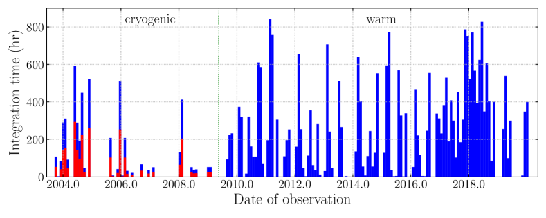
All observations described here were made with IRAC. In brief, IRAC is a four-channel array camera on the Spitzer Space Telescope, observing simultaneously four fields slightly separated on the sky at , , , and , known as channels 1–4, respectively. Spitzer science observations began in August 2003 but observations in channels 3 and 4 ceased once the on-board cryogen was exhausted (May 15, 2009). During the following ‘warm mission’ phase, channels 1 and 2 continued to operate until the end of operations in late January 2020, albeit with somewhat lower but still comparable performance. The earliest observations presented here are archival observations that were obtained in September 2003; the observations of the dedicated Capak program began in 2017 and the ones of the dedicated Scarlata program began in 2019. The dedicated observations continued until January 2020, shortly before the shutdown of the satellite. Figure 1 shows a histogram of the integration time accumulated in bins of 30 days over the observing period. These observations account for almost 1.5 million frames, a total integration time of hr, all channels combined, and a total on-target time, omitting overheads, of just over hr, or nearly 1.8 yr, which is approximately 11 % of the Spitzer Space Telescope mission time.
For our dedicated observations of EDF-N, EDF-S and EDF-F we adopted a consistent observing strategy that comprises blocks of maps with a step size of 310″, a large three-point dither pattern and four repeats per position. Each block covers a region with a coverage of s exposures per pixel. The block centres are offset between passes in order to ensure uniform coverage and enable self-calibration. Each block forms an AOR, or Astronomical Observation Request, in IRAC jargon. All other data included in our processing is archival data. It was obtained with a variety of observing strategies which we did not investigate in detail and which we do not attempt to summarise here. In Appendix C we list the Program IDs of all the observations processed; in bold the ones of our dedicated observations. The combination of the archival data with our own dedicated data produces a spatially variable depth in most fields; this is discussed further in Sect. 4.
A total of 292 IRAC observing programs are used in this work. Table 1 lists the ten largest programs in terms in terms of observing time together with the PI of the program, the field concerned and program’s total integration time.
| PID | Principal Investigator | Field | Time (hr) | Reference |
|---|---|---|---|---|
| 61041 | Giovanni Fazio | XMM | 847 | SEDS; Ashby et al. (2013) |
| 61040 | Giovanni Fazio | HDFN | 914 | SEDS; Ashby et al. (2013) |
| 14235 | Claudia Scarlata | EDF-S | 1086 | this paper |
| 169 | Mark Dickinson | HDFN | 1104 | GOODS; Labbé et al. (2015) |
| 10042 | Peter Capak | XMM | 2033 | this paper |
| 90042 | Peter Capak | COSM | 2167 | this paper |
| 13094 | Ivo Labbe | COSM | 2483 | GOODS; Labbé et al. (2015) |
| 11016 | Karina Caputi | COSM | 3021 | SMUVS; Ashby et al. (2013) |
| 13058 | Peter Capak | EDF-F | 3162 | this paper |
| 13153 | Peter Capak | EDF-N | 4625 | this paper |
All observations are summarised in Table 2 which gives, for each field and channel, the number of frames (Data Collection Events or DCEs in IRAC terminology) used to produce the mosaics (note that this can be lower than the number of frames downloaded as some were discarded, see Sect. 3) together with the total observing time. For channels 1 and 2, on the left side of the table, the information is subdivided into the cryogenic part and the warm part of the mission.
| Field | Ch. | cryo | warm | total | Ch. | total | |||||
|---|---|---|---|---|---|---|---|---|---|---|---|
| Num | Time | Num | Time | Num | Time | Num | Time | ||||
| EDF-N | 1 | 5 859 | 52 | 113 521 | 2 380 | 119 380 | 2 432 | 3 | 5 856 | 52 | |
| EDF-N | 2 | 5 857 | 52 | 113 204 | 2 467 | 119 061 | 2 519 | 4 | 7 667 | 50 | |
| EDF-F | 1 | 14 299 | 363 | 105 781 | 2 672 | 120 080 | 3 035 | 3 | 14 301 | 363 | |
| EDF-F | 2 | 14 299 | 363 | 105 779 | 2 764 | 120 078 | 3 127 | 4 | 29 686 | 352 | |
| EDF-S | 1 | n/a | n/a | 21 982 | 534 | 21 982 | 534 | 3 | n/a | n/a | |
| EDF-S | 2 | n/a | n/a | 21 982 | 552 | 21 982 | 552 | 4 | n/a | n/a | |
| COSMOS | 1 | 7 014 | 185 | 191 072 | 4 886 | 198 086 | 5 071 | 3 | 7 011 | 185 | |
| COSMOS | 2 | 7 013 | 185 | 191 031 | 5 052 | 198 044 | 5 237 | 4 | 13 894 | 179 | |
| EGS | 1 | 4 673 | 192 | 44 101 | 551 | 48 774 | 743 | 3 | 4 672 | 192 | |
| EGS | 2 | 4 673 | 192 | 44 101 | 569 | 48 774 | 761 | 4 | 14 535 | 186 | |
| HDFN | 1 | 6 253 | 298 | 36 485 | 930 | 42 738 | 1 228 | 3 | 6 252 | 298 | |
| HDFN | 2 | 6 253 | 298 | 36 485 | 962 | 42 738 | 1 260 | 4 | 22 496 | 288 | |
| XMM | 1 | 10 264 | 154 | 98 027 | 2 410 | 108 291 | 2 564 | 3 | 10 265 | 154 | |
| XMM | 2 | 10 265 | 154 | 98 030 | 2 495 | 108 295 | 2 649 | 4 | 14 321 | 151 | |
3 Processing
3.1 Pre-processing and calibration
Processing begins with the Level 1 data products generated by the Spitzer Science Center via their ‘Basic Calibrated Data’ pipeline (Lowrance et al. 2016), which were downloaded from the NASA/IPAC Infrared Science Archive (IRSA333https://irsa.ipac.caltech.edu). They have had all well-understood instrumental signatures removed, have been flux-calibrated in units of MJy sr-1, and are delivered with an uncertainty image and a mask image; they are described in detail in the IRAC Instrument Handbook444https://irsa.ipac.caltech.edu/data/SPITZER/docs/irac/iracinstrumenthandbook/home. More precisely, we begin from the ‘corrected basic calibration data’ products, which have file extensions .cbcd for the image, .cbunc for the uncertainty, and .bimsk for the mask. The files are grouped by AORs, namely sets of a few to several hundred DCEs obtained sequentially. All frames are pixels, the pixels are wide, and the image file header contains the photometric solution and an initial astrometric solution.
The processing is done region by region. A first pass over the files is used to check the headers for completeness and to discard a few incomplete AORs, which accounts for most of the differences in the number of frames listed in Table 2 between channels 1 and 2, or 3 and 4. This is followed by the correction of the ‘first frame’ bias effect555https://irsa.ipac.caltech.edu/data/SPITZER/docs/irac/iracinstrumenthandbook/26/. Next, the positions and magnitudes of WISE ((Wright et al. 2010), (Mainzer et al. 2011)) and Gaia DR2 (Gaia Collaboration et al. 2018) sources falling within the field are downloaded. The Gaia sources are first ‘projected’ to their location at the time of the observations using the Gaia proper motions. Next they are identified on each IRAC frame, their observed fluxes and positions determined in each frame using the APEX software (the point-source extractor in MOPEX666https://irsa.ipac.caltech.edu/data/SPITZER/docs/dataanalysistools/tools/mopex/) in forced-photometry mode, and the positions are used to update the astrometric solution of each frame. There are typically 30–40 Gaia DR2 sources available for each frame. In channels 1 and 2 most of them are detected and used for the astrometric correction. In the longer-wavelength channels 3 and 4 only a few sources in total are detected and usable but that is still sufficient to determine an astrometric solution with negligible distortion as shown in Sect. 4.2.
An attempt was made to subtract bright stars in order to recover faint sources in their wings. For each AOR a model star built from the template PSFs described in the IRAC Instrument Handbook777https://irsa.ipac.caltech.edu/data/SPITZER/docs/irac/iracinstrumenthandbook/19/ (see Fig. 4.9 there) is scaled to the median of the fluxes of the star measured in that AOR, and is subtracted from each frame (of the AOR). Different templates are available for each filter and separately for the cryogenic and the warm missions. While this procedure worked quite well for moderately bright stars (which are of course the vast majority and which represent only a small loss in area), it introduced significant artefacts around the (few) very bright stars in the final mosaics. These artefacts included diffraction spikes corrected only out to a certain distance (out to where the template extends beyond the frame), other edge effects, and the subtraction of the core of bright galaxies. For these reasons the bright-star subtraction was not performed and the bright stars are left as they are.
3.2 Stacking and image combination
In the next step we compute a median image for all frames within an AOR which corrects for persistence in the detectors and also for any residual first-frame pattern that introduces structure in the background. In parallel, a background map is also created by iteratively clipping objects and masking them, and finally that background is subtracted from each frame of the AOR.
The final processing steps consist of resampling the background-subtracted frames onto a common grid with a scale of , i.e., half the instrument pixel size, that covers all data in all channels and which is the same in all channels. We experimented with two MOPEX interpolation schemes to produce our final mosaics. We first tried the ‘drizzling’ (Fruchter & Hook 2002) scheme in which the final value of the output pixels is computed by considering the contribution of each input pixel in a smaller pixel grid in the output image. This procedure has excellent noise properties (it does not suffer from correlated pixels) when many input frames are available, but with few input frames it can produce artefacts in the output images. The second, simpler approach is to compute the value of each output pixel as a linear combination of the input pixel values. Although this procedure produces correlated noise, it works reliably for all the fields considered in this work which can have widely varying numbers of input images. Noise correlations can be estimated through simulations or by comparing sources in our drizzled and non-drizzled images. These comparisons show that the linear interpolation procedure leads to an underestimation of aperture magnitude errors by while the magnitudes themselves are unaffected.
Next, we use MOPEX to produce an average-combined image while rejecting outliers and excluding masked regions. The stacking pipeline also produces the following ancillary characterisation maps: (1) an uncertainty map produced by stacking the input uncertainty maps using the same shifts as for the signal stack, (2) a coverage map giving the number of frames contributing to each pixel, and (3) an exposure time map giving the total exposure time per pixel. As the exposure times are not the same for all the observing programmes, these last two maps are not simply scaled versions of each other.
3.3 On the spatial variation of the PSF in the stacks
The observations described here were made at many different satellite position angles (PAs), and thus when the images are stacked they must be rotated back to North upwards. This has the effect of rotating the PSF, which is fixed in the satellite’s reference frame. Since the PSF is not rotationally symmetric, due in particular to the diffraction spikes, the stacked image of a star will depend on when it was observed. As all parts of the stack were not observed at the same time (or at the same PA), the PSF varies spatially in the stack.
The COSMOS field, which is near the Equator, was observable only at specific times and therefore with a very restricted range of PAs; the PSF in the COSMOS stacks is thus quite homogeneous. But in the EDF-N, which was in a continuous viewing zone, observations were obtained at many different PAs, yielding more complicated and more spatially variable PSF. This effect is very important for PSF-based photometry: the PSF at each position of the stack has to be reconstructed by stacking the nominal PSF at the PAs of the observations at that position, as did e.g., Labbe et al. (2015) for the GOODS-South and HUDF fields, and also Weaver et al. (submitted) for the production of the COSMOS2020 catalogue. The latter used the PRFmap code by Andreas Faisst, available at https://github.com/cosmic-dawn/prfmap for that purpose. While doing such photometry is beyond the scope of this paper, we nevertheless provide, for each stack, a table of the PAs of each frame used in the stack. For completeness those tables also contain the frame coordinates, the MJD of the observation, and the exposure time; see Appendix A for more details.
3.4 Products
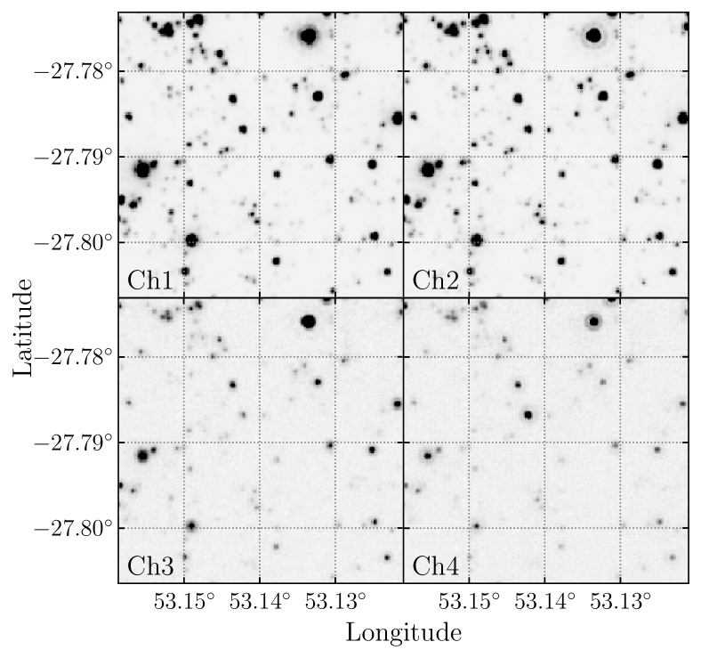
As an example of the data quality, Fig. 2 shows a zoomed section of the EDF-F mosaic in the four channels near the region of maximum coverage. We do not provide here figures of the full mosaics as they would be physically too small to show anything informative other than the overall coverage.
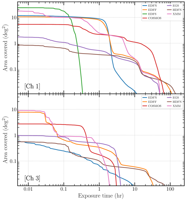
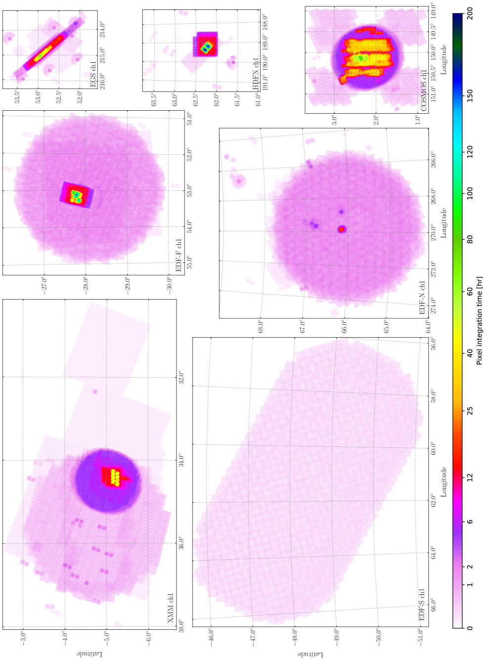
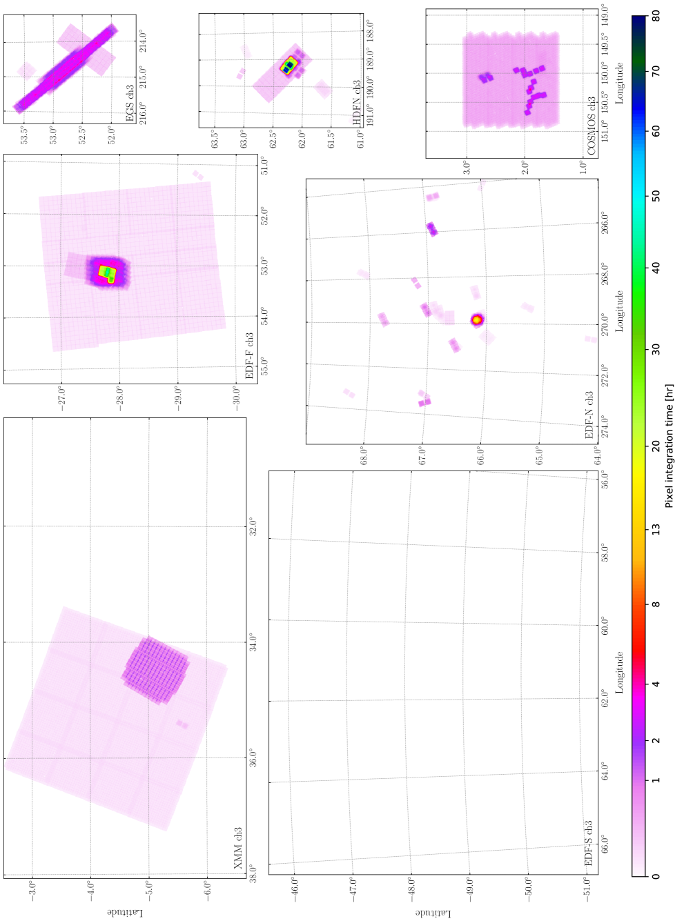
Maps of the integration time per pixel for channels 1 and 3 of all the fields are presented in Appendix B. Since channel 2 is observed together with channel 1, and similarly for channels 4 and 3, the paired channels have very similar coverage, albeit slightly shifted in position. The 10 deg2 circular area of EDF-N and EDF-F and the 20 deg2 pill-shaped area of EDF-S are easily seen on those figures. Also, and with the exception of EDF-S, for which there are only observations done specifically for this programme and no archival data, the integration time per pixel, and consequently the depth reached, is far from uniform, with only a small part of the total area of each field having been observed for more than a few hours. In fact, the median integration time per pixel is larger than 1 hr for only two fields. Table 3 gives the median and maximum pixel integration time for each field and each channel.
| Field | ch1 | ch2 | ch3 | ch4 | ||||
|---|---|---|---|---|---|---|---|---|
| COSMOS | 0.51 | 93.7 | 0.50 | 97.1 | 0.38 | 5.1 | 0.38 | 5.5 |
| EDF-F | 1.33 | 199.7 | 1.33 | 149.5 | 0.03 | 47.3 | 0.03 | 54.2 |
| EDF-N | 1.47 | 23.4 | 1.56 | 21.3 | 0.04 | 20.4 | 0.04 | 19.6 |
| EDF-S | 0.13 | 0.5 | 0.16 | 0.5 | – | – | – | – |
| EGS | 0.16 | 71.1 | 0.16 | 71.6 | 0.93 | 5.4 | 0.95 | 4.8 |
| HDFN | 0.16 | 236.2 | 0.16 | 224.4 | 0.13 | 91.2 | 0.13 | 95.2 |
| XMM | 0.31 | 65.9 | 0.33 | 67.1 | 0.04 | 2.0 | 0.04 | 2.0 |
That variation of area covered as a function of exposure time for channels 1 and 3 and for all fields is shown graphically in Fig. 3 which presents a cumulative histogram of the area covered vs. exposure time. The intersection of the curve with the vertical axis thus gives the total area covered for that field and these areas are also listed in Table 4. EDF-S is the most uniformly observed field and it covers the largest area, but it is also the shallowest, with only 0.1 hr per pixel on average, and it is also the only field with no channel 3 and 4 data. EDF-F and EDF-N reach the target coverage of 10 deg2 with about 1 hr of exposure time, with the latter showing deeper coverage over smaller zones. The other fields were covered by many observing programs with different objectives and which covered specific areas to different depths. The combination of these programs with our own yields a curve with many plateaus. Finally, there are a few small parts of the EDF-F and HDFN fields that have more than 100 hr of exposure time.
| Field | RA | Dec | ch1 | ch2 | ch3 | ch4 | |
|---|---|---|---|---|---|---|---|
| EDF-N | 11.74 | 11.54 | 0.61 | 0.62 | |||
| EDF-F | 10.52 | 11.05 | 7.78 | 7.77 | |||
| EDF-S | 23.60 | 23.14 | – | – | |||
| COSMOS | 5.37 | 5.46 | 2.72 | 2.72 | |||
| EGS | 1.76 | 1.80 | 0.97 | 0.98 | |||
| HDFN | 0.91 | 0.91 | 0.57 | 0.63 | |||
| XMM | 17.54 | 17.48 | 9.09 | 9.10 |
3.5 Final sensitivities
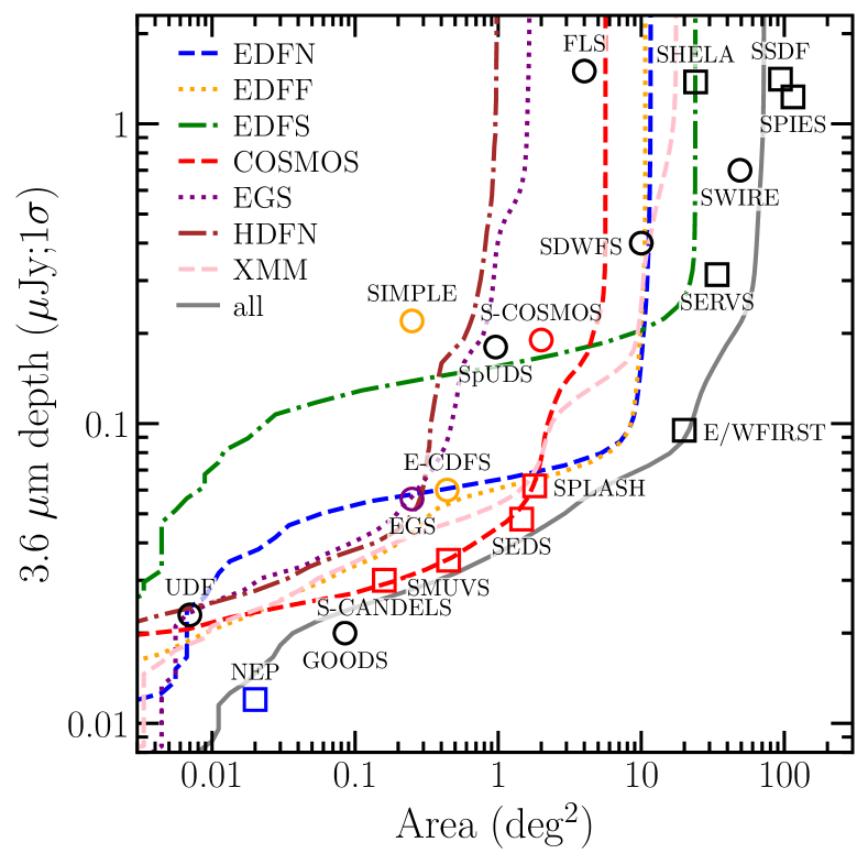
We estimate the sensitivities of the stacked images by measuring the flux in circular diameter apertures randomly placed across each image after masking the regions with detected objects using the SExtractor (Bertin & Arnouts 1996) segmentation map. The sensitivity is then computed as the standard deviation of these fluxes (3 clipped). This procedure is done in pixel cells (4 arcmin2). Figure 4 shows the cumulative area covered as a function of sensitivity for the channel 1 mosaics. Note the similarity between this figure and the top panel of Fig. 3 once the latter is rotated by 90 degrees. The solid line shows our total depth, summed over all our survey fields. Also shown in the figure are the published sensitivities of the surveys that are included in our data and analyses. Generally, our measured sensitivities are consistent with literature measurements for surveys of equivalent exposure time.
4 Validation and quality control
As part of our validation process we compare photometry and astrometry of sources in our stacks with reference catalogues and also extract number counts that can be compared to previous works.
4.1 Catalogue extraction
We begin by extracting source catalogues from the channels 1 and 2 stacks of all fields using SExtractor. We adopt the usual approach of searching for objects that contain a minimum number of connected pixels above a specified noise threshold (in this case ) and measuring their aperture magnitudes. In the case of our moderately deep IRAC data, where many sources are blended due to the large IRAC PSF, this approach is known to miss faint sources. However, these faint sources are not required for our quality assessment purposes and a shallower catalogue is entirely sufficient. SExtractor estimates a global background on a grid with mesh size of pixels (recall that pixels are wide). This background is smoothed with a pixel Gaussian kernel with . For each source, the flux is measured within a circular aperture of diameter and a local background is estimated within an annulus of width pixels around the isophotal limits. The measured fluxes were converted from MJy/sr to AB magnitude using a zero-point of (which accounts for a zero-magnitude flux of 3631 Jy and a pixel size of 888https://irsa.ipac.caltech.edu/data/SPITZER/docs/irac/iracinstrumenthandbook/19/), and the latter were converted to total magnitude using the aperture corrections given in the IRAC Instrument Handbook for the warm mission ( and for channel 1 and channel 2 respectively), which covers the vast majority of the data, while the correction for the cryogenic mission differs at only the 1–2% level999https://irsa.ipac.caltech.edu/data/SPITZER/docs/irac/calibrationfiles/ap_corr_warm/. A list of relevant SExtractor parameters used for the catalogue extraction can be found in Table 5.
| Parameter name | Value |
|---|---|
| DETECT_MINAREA | 5 |
| DETECT_MAXAREA | 1000000 |
| THRESH_TYPE | RELATIVE |
| DETECT_THRESH | 2 |
| ANALYSIS_THRESH | 2 |
| FILTER_NAME | gauss_2.5_5x5.conv |
| DEBLEND_NTHRESH | 32 |
| DEBLEND_MINCONT | 0.00001 |
| BACK_SIZE | 32 |
| BACKPHOTO_THICK | 32 |
| BACK_FILTERSIZE | 3 |
| BACKPHOTO_TYPE | LOCAL |
| MAG_ZEROPOINT | 21.58 |
| PHOT_AUTOPARAMS | 2.5,5.0 |
| PIXEL_SCALE | 0.60 |
4.2 Astrometric and photometric validation
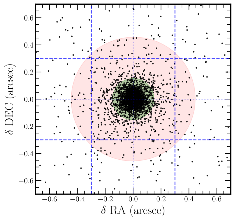
Using the catalogues extracted above, we evaluate the astrometric accuracy of our stacked images. For each field we cross-match sources with magnitude within of their counterparts in the Gaia DR2 catalogue. This magnitude range was adopted to ensure only bright, non-blended sources were chosen. We now present a detailed analysis for EDF-N but other fields are similar.
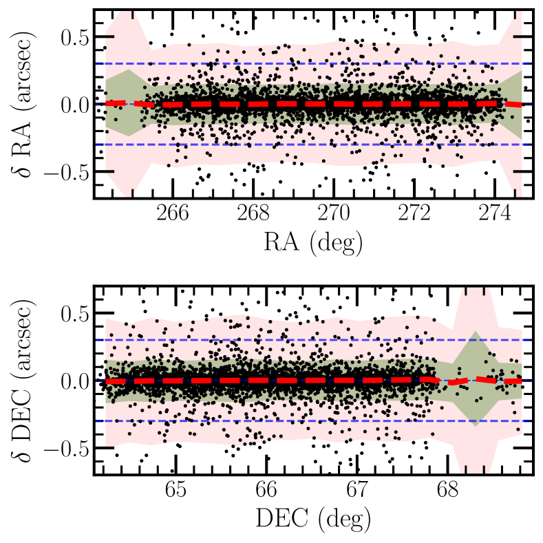
Figure 5 shows the difference between reference and measured coordinates (for clarity, only one point in ten is shown). The heavy blue dashed line gives the size of one pixel in the stacked image (which is half the size of the instrument pixel). Similarly (again showing only one in ten points), Fig. 6 shows, for each coordinate, the difference between the reference and the measured value as a function of position along the other coordinate. The thick red dashed line shows a running median computed over a bin containing 20 points. The flatness of this line indicates that there is no significant spatial variation in astrometric precision. Considering all fields, we find that the 1 precision (measured as the RMS of the difference between positions in our catalogue and those in Gaia DR2) is . Furthermore, the median value is always , with the exception of the sparsely-covered HDF-N field where it is .
These measurements demonstrate that the astrometric solutions have been correctly applied to the individual images and that the combined images are free of residuals on a scale much smaller than an individual mosaic pixel, which is more than sufficient to measure precise infrared and optical-infrared colours.
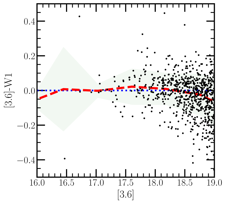
Finally, we perform a simple check on the photometric calibration of our mosaics. As described previously, individual images are photometrically calibrated by the Spitzer Science Center (SSC). Following the validation procedures outlined by the SSC, we compare magnitudes of objects in our catalogues with those in the WISE survey. Because of the difference between the WISE W1 and IRAC channel 1 filter profiles, we select objects with . Figure 7 shows the magnitude difference for the EDF-N field, and the agreement is excellent. Further comparisons with photometric measurements in previous COSMOS IRAC surveys can be found in the Appendix of Weaver et al.
4.3 Magnitude number counts
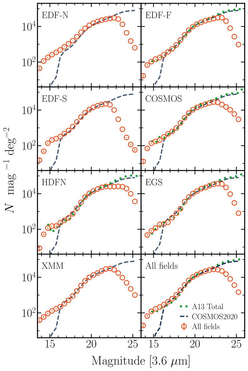
We compute the differential number counts in channel 1 in each field using the corrected aperture magnitudes. Since the IRAC PSF is too large to perform morphological source classification, we simply include all objects detected. These are shown in Fig. 8, where the red circles with uncertainties present our measurements and the lines show the number counts from the literature; the bottom-right panel shows the mean of all fields. We compare our number counts with those presented in Ashby et al. (2013) who also surveyed many of our fields and also with those computed using the new COSMOS2020 photometric catalogue (Weaver et al., submitted) which we use as a reference.
There is a general agreement in the number counts in all the fields with Ashby et al. (2013) and COSMOS2020 for . At brighter magnitudes the COSMOS2020 counts drop off as bright sources were not included. At fainter magnitudes, our aperture-based catalogues are confusion-limited and thus incomplete. Conversely, the COSMOS2020 catalogue, which uses a high-resolution prior for the detection and a profile-fitting method for the measurement, is complete up to significantly fainter magnitudes.
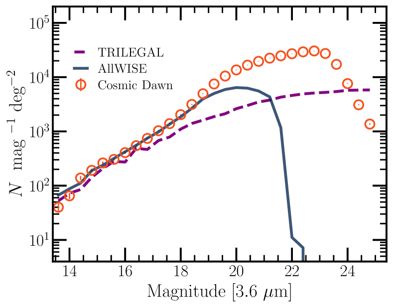
EDF-N counts are slightly higher than the other fields at bright magnitudes. To investigate this difference we simulated a stellar catalogue of centred on EDF-N using TRILEGAL (Girardi et al. 2005) and compared counts from this simulated catalogue with our observations, shown in Fig. 9. At bright magnitudes, where stars are expected to outnumber galaxies, our counts are in reasonable agreement with TRILEGAL predictions, and in excellent agreement with the number counts extracted from the AllWISE (Wright et al. 2010) catalogue for this field. These comparisons indicate that the difference between EDF-N and other fields is largely due to the higher density of stellar sources in there, consistent with its lower Galactic latitude.
5 Summary
We have presented the Spitzer/IRAC mid-infrared component of the Cosmic Dawn Survey: an effort to complement the Euclid mission’s observations of deep and calibration fields with deep longer-wavelength data to enable high redshift legacy science.
The survey consists of two major new programs covering the three Euclid deep fields (EDF-N, EDF-F and EDF-S) and a homogeneous reprocessing of all existing data in Euclid’s four calibration fields (COSMOS, XMM, EGS and HDFN). We have processed new data together with all relevant archival data to produce mosaics of these fields covering a total of deg2 in IRAC channels 1 and 2. Furthermore, the new mosaics are tied to the Gaia astrometric reference system. The MIR data will be essential for a wide range of legacy science with Euclid, including improved star/galaxy separation, more accurate photometric redshifts, determination of stellar masses of galaxies, and the construction of complete galaxy samples at with well understood selection effects.
We validated our final products by comparing catalogues extracted from channels 1 and 2 to external catalogues. In all fields, comparing with Gaia DR2, the residual astrometric uncertainty for sources with total magnitudes is around (). Our photometric measurements are in excellent agreement with WISE photometry and our number counts are consistent with previous determinations.
The Cosmic Dawn Survey Spitzer survey presented here represents the first essential step in assembling the required multi-wavelength coverage in the Euclid deep fields which are set to become some of the most important fields in extragalactic astronomy for the coming decade. Since the Spitzer mission has finished, and all available data in these fields have been processed with the latest reduction pipeline, the resulting mosaics will remain the deepest and widest MIR imaging survey for the foreseeable future. No existing or approved future observatories are capable of obtaining such data. While JWST is more sensitive and has higher spatial resolution at these wavelengths, its mapping speed is too slow to cover comparable degree-scale areas.
In the context of the Cosmic Dawn Survey, several programs are currently underway to add data at other wavelengths to the Euclid deep fields and calibration fields. In particular deep optical data in the EDF-N and EDF-F are currently being obtained with the Subaru’s Hyper-Suprime-Cam instrument as part of the Hawaii-Two-0 program (McPartland et al., in prep). These fields are also being targeted with high spatial resolution millimeter observations as part of the planned Large-scale Structure Survey with the Toltech Camera101010 http://toltec.astro.umass.edu/ on the Large Millimeter Telescope (LMT Pope et al. 2019). A deep -band survey is also underway with the CFHT (Zalesky et al., in prep). EDF-S is being covered with K-band observations from the VISTA telescope (Nonino et al., private communication), and planning is ongoing to obtain optical data with the Vera C. Rubin Observatory.
The Cosmic Dawn Survey Spitzer mosaics and associated products described here can be downloaded from the IRSA web site, Appendix A gives the details of the download site and the naming convention used. The community is encouraged to make use of them for their science.
Acknowledgements.
We thank the MOPEX support team for fixing issues that appeared when combining large numbers of files. This publication is based on observations made with the Spitzer Space Telescope, which is operated by the Jet Propulsion Laboratory, California Institute of Technology under a contract with NASA, and has made use of the NASA/IPAC Infrared Science Archive, which is funded by the National Aeronautics and Space Administration and operated by the California Institute of Technology. This publication has also made use of data from the European Space Agency (ESA) mission Gaia (https://www.cosmos.esa.int/gaia), processed by the Gaia Data Processing and Analysis Consortium (DPAC, https://www.cosmos.esa.int/web/gaia/dpac/consortium). Funding for the Gaia Data Processing and Analysis Consortium (DPAC) has been provided by national institutions, in particular the institutions participating in the Gaia Multilateral Agreement. This publication makes use of data products from the Wide-field Infrared Survey Explorer (WISE), which is a joint project of the University of California, Los Angeles, and the Jet Propulsion Laboratory/California Institute of Technology, funded by the National Aeronautics and Space Administration. H.J.McC. acknowledges support from the PNCG. This work used the CANDIDE computer system at the IAP supported by grants from the PNCG and the DIM-ACAV and maintained by S. Rouberol. S.T. and J.W. acknowledge support from the European Research Council (ERC) Consolidator Grant funding scheme (project ConTExt, grant No. 648179). I.D. has received funding from the European Union’s Horizon 2020 research and innovation programme under the Marie Skłodowska-Curie grant agreement No. 896225. The Cosmic Dawn Center is funded by the Danish National Research Foundation under grant No. 140. H.Hildebrandt is supported by a Heisenberg grant of the Deutsche Forschungsgemeinschaft (Hi 1495/5-1) as well as an ERC Consolidator Grant (No. 770935).The Euclid Consortium acknowledges the European Space Agency and a number of agencies and institutes that have supported the development of Euclid, in particular the Academy of Finland, the Agenzia Spaziale Italiana, the Belgian Science Policy, the Canadian Euclid Consortium, the Centre National d’Etudes Spatiales, the Deutsches Zentrum für Luft- und Raumfahrt, the Danish Space Research Institute, the Fundação para a Ciência e a Tecnologia, the Ministerio de Economia y Competitividad, the National Aeronautics and Space Administration, the National Astronomical Observatory of Japan, the Netherlandse Onderzoekschool Voor Astronomie, the Norwegian Space Agency, the Romanian Space Agency, the State Secretariat for Education, Research and Innovation (SERI) at the Swiss Space Office (SSO), and the United Kingdom Space Agency. A complete and detailed list is available on the Euclid web site (http://www.euclid-ec.org).References
- Aihara et al. (2011) Aihara, H., Allende Prieto, C., An, D., et al. 2011, ApJS, 193, 29
- Ashby et al. (2018) Ashby, M. L. N., Caputi, K. I., Cowley, W., et al. 2018, ApJS, 237, 39
- Ashby et al. (2013) Ashby, M. L. N., Willner, S. P., Fazio, G. G., et al. 2013, ApJ, 769, 80
- Beckwith et al. (2006) Beckwith, S. V. W., Stiavelli, M., Koekemoer, A. M., et al. 2006, AJ, 132, 1729
- Bell & de Jong (2001) Bell, E. F. & de Jong, R. S. 2001, ApJ, 550, 212
- Bertin & Arnouts (1996) Bertin, E. & Arnouts, S. 1996, A&AS, 117, 393
- Bouwens et al. (2019) Bouwens, R. J., Stefanon, M., Oesch, P. A., et al. 2019, ApJ, 880, 25
- Bowler et al. (2020) Bowler, R. A. A., Jarvis, M. J., Dunlop, J. S., et al. 2020, MNRAS, 493, 2059
- Brammer et al. (2012) Brammer, G. B., van Dokkum, P. G., Franx, M., et al. 2012, ApJS, 200, 13
- Bridge et al. (2019) Bridge, J. S., Holwerda, B. W., Stefanon, M., et al. 2019, ApJ, 882, 42
- Caputi et al. (2015) Caputi, K. I., Ilbert, O., Laigle, C., et al. 2015, ApJ, 810, 73
- Davidzon et al. (2017) Davidzon, I., Ilbert, O., Laigle, C., et al. 2017, A&A, 605, A70
- Fazio et al. (2004) Fazio, G. G., Hora, J. L., Allen, L. E., et al. 2004, ApJS, 154, 10
- Fruchter & Hook (2002) Fruchter, A. S. & Hook, R. N. 2002, PASP, 114, 144
- Gaia Collaboration et al. (2018) Gaia Collaboration, Brown, A. G. A., Vallenari, A., et al. 2018, A&A, 616, A1
- Giavalisco et al. (2004) Giavalisco, M., Ferguson, H. C., Koekemoer, A. M., et al. 2004, ApJ, 600, L93
- Girardi et al. (2005) Girardi, L., Groenewegen, M. A. T., Hatziminaoglou, E., & da Costa, L. 2005, A&A, 436, 895
- Kauffmann et al. (2020) Kauffmann, O. B., Le Fèvre, O., Ilbert, O., et al. 2020, A&A, 640, A67
- Labbé et al. (2015) Labbé, I., Oesch, P. A., Illingworth, G. D., et al. 2015, ApJS, 221, 23
- Laureijs et al. (2011) Laureijs, R., Amiaux, J., Arduini, S., et al. 2011, arXiv e-prints, arXiv:1110.3193
- Le Fèvre et al. (2015) Le Fèvre, O., Tasca, L. A. M., Cassata, P., et al. 2015, A&A, 576, A79
- Legrand et al. (2019) Legrand, L., McCracken, H. J., Davidzon, I., et al. 2019, MNRAS, 486, 5468
- Lowrance et al. (2016) Lowrance, P. J., Carey, S. J., Surace, J. A., et al. 2016, in Space Telescopes and Instrumentation 2016: Optical, Infrared, and Millimeter Wave, ed. H. A. MacEwen, G. G. Fazio, M. Lystrup, N. Batalha, N. Siegler, & E. C. Tong, Vol. 9904, International Society for Optics and Photonics (SPIE), 1853 – 1860
- Mainzer et al. (2011) Mainzer, A., Grav, T., Bauer, J., et al. 2011, The Astrophysical Journal, 743, 156
- Pérez-González et al. (2008) Pérez-González, P. G., Rieke, G. H., Villar, V., et al. 2008, ApJ, 675, 234
- Pope et al. (2019) Pope, A., Aretxaga, I., Hughes, D., Wilson, G., & Yun, M. 2019, in American Astronomical Society Meeting Abstracts, Vol. 233, American Astronomical Society Meeting Abstracts #233, 363.20
- Scaramella et al. (2021) Scaramella, R., Amiaux, J., Mellier, Y., et al. 2021, arXiv e-prints, arXiv:2108.01201
- Trac et al. (2008) Trac, H., Cen, R., & Loeb, A. 2008, ApJ, 689, L81
- Werner et al. (2004) Werner, M. W., Roellig, T. L., Low, F. J., et al. 2004, ApJS, 154, 1
- Wright et al. (2010) Wright, E. L., Eisenhardt, P. R. M., Mainzer, A. K., et al. 2010, AJ, 140, 1868
Appendix A Delivered data products
The new mosaics and associated products can be obtained from the IRSA website at https://irsa.ipac.caltech.edu/data/SPITZER/Cosmic_Dawn (ATTN: the products will become available once the paper is accepted; the URL may be updated at publication time). The file naming convention for the stacks is as follows:
CDS_{field}_ch{N}_{type}_v24.fits
where field is the field name, N is the channel number, and type is one of
-
ima: for the flux image, -
cov: for the coverage in terms of number of frames used to build each pixel of the mosaic, -
tim: for the exposure time in sec of the pixel, and -
unc: for the uncertainty as determined from the standard deviation of the image pixels that contributed to the mosaic pixel.
Also, Table 6 gives the precise J2000 coordinates of the field tangent point in decimal degrees, the reference pixel corresponding to that tangent point, and size, in pixels, of the mosaics. These values are the same for all channels of a field and for all the ancillary images. The pixel scale is per pixel for all mosaics.
| Field | Longitude | Latitude | -size | -size | -ref.pix | -ref.pix |
|---|---|---|---|---|---|---|
| EDF-N | 269.485804 | 66.590708 | 27 410 | 30 148 | 13 705.55 | 15 074.53 |
| EDF-F | 53.062008 | –28.205431 | 23 751 | 26 204 | 11 876.02 | 13 102.29 |
| EDF-S | 61.301724 | –48.496065 | 41 676 | 33 976 | 20 838.59 | 16 988.50 |
| COSMOS | 150.178292 | 2.220994 | 15 440 | 17 804 | 7 720.46 | 8 902.40 |
| EGS | 214.781187 | 52.720882 | 11 278 | 13 649 | 5 639.32 | 6 824.97 |
| HDFN | 189.405434 | 62.373754 | 11 813 | 1 979 | 5 907.03 | 8 489.78 |
| XMM | 34.101249 | –4.598575 | 47 583 | 25 022 | 23 791.97 | 12 511.69 |
The tables with the observation date, coordinates, position angles, and exposure times of the input frames are provided in IPAC format and are gzipped to reduce their size. Their names are as follows:
CDS_{field}_ch{N}_info_v24.tbl.gz
The first few lines of the table for channel 1 of the EGS field are as follows:
  |          MJD|              RA|             DEC|               PA|ExpTime|
  |       double|          double|          double|           double| double|
  |          day|             deg|             deg|              deg|    sec|
  |         null|            null|            null|             null|   null|
   53822.6296863 214.458364468008 51.9912156620541 -126.246899270774     0.4
   53822.6297117 214.458364468008 51.9912156620541 -126.247055616923    10.4
   53822.6298641 214.458364468008 51.9912156620541 -126.246928305428    96.8
   53822.6312156 214.383044470269 52.0556500561605 -126.304483006668    96.8
The coordinates are in degrees of longitude and latitude (Equatorial, J2000) and the PAs are measured eastward of North.
Appendix B Coverage maps
Figures 10 and 11 show the full set of pixel exposure time maps for channels 1 and 3; channels, 2 and 4 are similar though slightly shifted in location. A square root scaling is applied in order to emphasise the differences at the low levels, and the same maximum is used for all fields in each channel. As EDF-S was not observed in channel 3, a blank field is placed there.
Appendix C PID numbers
Table 7 lists the Spitzer Program-IDs (PIDs) of all the observations processed here. In bold the ones of the observing programmes that we planned for this work, the others are of the other archival observations that we reprocessed.
| Field | PIDs |
|---|---|
| EDF-N | 68 609 613 618–624 1101 1125 1188 1189 1191–-1200 1317 1334 1600–-1700 1910–-1949 1951 1953–1961 1963–1983 2314 3286 3329 3672 10147 11161 13153 20466 30432 40385 60046 70062 70162 80109 80113 80243 80245 90209 |
| EDF-F | 81 82 184 194 2313 11080 13058 20708 30866 40058 60022 61009 61052 70039 70145 70204 80217 |
| EDF-S | 14235 |
| COSMOS | 10159 11016 12103 13094 13104 14045 14081 14203 20070 40801 50310 61043 61060 70023 80057 80062 80134 80159 90042 |
| EGS | 8 10084 11065 11080 13118 20754 41023 60145 61042 80069 80156 80216 90180 |
| HDFN | 81 169 1304 10136 11004 11063 11080 11134 12095 13053 20218 30411 30476 40204 60122 60145 61040 61062 61063 70162 80215 |
| XMM | 181 3248 10042 11086 40021 60024 61041 61060 61061 70039 70062 80149 80156 80159 80218 90038 90175 90177 |