Regulation of star formation by large scale gravito-turbulence

Abstract

A simple model for star formation based on supernova (SN) feedback and gravitational heating via the collapse of perturbations in gravitationally unstable disks reproduces the Schmidt-Kennicutt relation between the star formation rate (SFR) per unit area, $\Sigma_{SFR}$, and the gas surface density, $\Sigma_{g}$, remarkably well. The gas velocity dispersion, $\sigma_{g}$, is derived self-consistently in conjunction with $\Sigma_{SFR}$ and is found to match the observations. Gravitational instability triggers “gravito-turbulence" at the scale of the least stable perturbation mode, boosting $\sigma_{g}$ at $\Sigma_{g}\mathrel{\hbox to0.0pt{\lower 4.0pt\hbox{\hskip 0.5pt$\sim$}\hss}\raise 1.0pt\hbox{$>$}}\,\Sigma_{g}^{\textrm{thr}}=50\,{\rm M}_{\odot}\,{\rm pc}^{-2}$, and contributing to the pressure needed to carry the disk weight vertically. $\Sigma_{SFR}$ is reduced to the observed level at $\Sigma_{g}\mathrel{\hbox to0.0pt{\lower 4.0pt\hbox{\hskip 0.5pt$\sim$}\hss}\raise 1.0pt\hbox{$>$}}\,\Sigma_{g}^{\textrm{thr}}$, whereas at lower surface densities, SN feedback is the prevailing energy source. Our proposed star formation recipes require efficiencies of order 1%, and the Toomre parameter, $Q$, for the joint gaseous and stellar disk is predicted to be close to the critical value for marginal stability for $\Sigma_{g}~{}\hbox to0.0pt{$<$\hss}{\lower 4.30554pt\hbox{$\sim$}}\,\Sigma_{g}^{\textrm{thr}}$, spreading to lower values and larger gas velocity dispersion at higher $\Sigma_{g}$.

1 introduction

Despite the complex interplay between a multitude of physical processes involved in galaxy formation, evolved galaxies exhibit remarkably simple scaling relations. One of these relations is the Schmidt-Kennicutt star formation law in disk galaxies $\Sigma_{SFR}=A\Sigma_{g}^{n}$ (Schmidt, 1959; Kennicutt, 1998) between the SFR per unit disk area, $\Sigma_{SFR}$, and the gas surface density, $\Sigma_{g}$. The universality of this relation over many decades in $\Sigma_{g},$ and its low scatter, indicate that it might be a consequence of a global quasi-equilibrium maintained over a long term evolution of galaxies.

If supernova (SN) feedback is the main driver for pressure, $p$, in the disk, then gravity-pressure balance in the vertical direction to the disk provides an appealing argument to derive a relation between $\Sigma_{SFR}$ and $\Sigma_{g}$. However, if $p\propto\Sigma_{SFR}$, vertical balance yields a near quadratic dependence on gas surface density, deviating strongly, especially at high $\Sigma_{g}$, from the $n\sim 3/2$ power inferred from the observed SK law. Further, a conceptual issue is that the pressure balance argument is phenomenologically persuasive but is insufficient to account both for the SFR and the turbulence velocity dispersion that supports the gas disk. Self-regulation of star formation and SN momentum injection are locally incomplete until interstellar turbulence is regulated. Specifically, pressure balance relies on, but does not specify, the turbulent gas velocity dispersion.

One problem is that there is no feedback loop between star formation and turbulent velocity dispersion in the simplest theory. SN-momentum regulation of star formation cannot self-consistently regulate the turbulence in the absence of dissipation physics. Moreover, observationally, there is indeed evidence that local star formation efficiency decreases with increasing turbulence inside molecular clouds (MCs) (Leroy et al., 2017; Querejeta et al., 2019).

In the absence of feedback, SFRs are well known to be far too high, both in disk galaxies as well as in spheroidal systems. Supernova-driven turbulence is the favored mechanism that regulates star formation (Joung & Mac Low, 2006).

Massive stellar feedback equally plays a role. Both OB winds and SN are essential in star–forming MCs to obtain the SFE required for the global SK law (Hopkins et al., 2011). More recent cosmological simulations of disk galaxies have improved resolution and focus on feedback via turbulent pressure in the inhomogeneous interstellar medium (ISM) (Gurvich et al., 2020).

Supernova-driven momentum deposition is the leading candidate for feedback in cosmological simulations of star-forming galaxies, but recovering the global SK relation and in particular its low observed scatter remains a challenge. Recent disk star formation simulations are consistent with vertical balance of disk weight and ISM pressure generated by momentum input from SN-regulated star formation, although only a quasilinear SK law with large scatter is produced. This is consistent with resolved galaxy studies on subkpc scales (Brucy et al., 2020) but does not account for the global SK law (Kim et al., 2020a).

SN-driven turbulence is inevitably significant in the densest star-forming regions such as the Central Molecular Zone of the MWG and more generally in starbursts (Seifried et al., 2018). This is less effective in forming ellipticals or in dwarfs. Nevertheless, in gas-rich systems, additional turbulent input seems to be required. One possibility is dynamically-induced turbulence (e.g. Fuchs & Von Linden, 1998; Semelin & Combes, 2000; Brucy et al., 2020), e.g. by external shear. Generally, SFRs in simulated disks with $\Sigma_{g}~{}\hbox to0.0pt{$<$\hss}{\lower 4.30554pt\hbox{$\sim$}}100\,{\rm M}_{\odot}\,{\rm pc}^{-2}$ can be explained by SN feedback alone, but mass loading and disk outflows remain a problem, suggesting that additional feedback is required (Smith et al., 2018). Incorporating pre-supernova massive star feedback enhances the energetic impact of SNe on the ISM (Lucas et al., 2020) and helps in producing outflows. But the presence of outlows does not seem to affect the SK inferred law as the SFR tends to adapt to the varying gas content (see Fig. 8 in Smith et al. (2018)). Multiphase modelling further boosts the outflow rates (Kim et al., 2020b).

Self-gravity, halo gravity, magnetic fields, radiation, stellar winds, cosmic rays, and SN feedback all contribute to the energy stored in galactic disks. The interplay between these factors dictates the stability of the gaseous disk component and its susceptibility to form stars. Krumholz & Burkhart (2016) and Krumholz et al. (2018) consider a model where gravito-turbulence is sustained by gravitational energy released via inflow of disk gas mass. Inward mass transport is detected in the outer parts of the disks of some galaxies in the HI Nearby Galaxy Survey (Schmidt et al., 2016). This model exploits vertical gravity-pressure equilibrium and energy balance between energy injection and dissipation. Turbulence driven by both gas transport and SN feedback is needed to account for observations of the SFR and velocity dispersion (see also Yu et al., 2021).

Even in the absence of star formation, the growth and collapse of perturbations in a gravitationally unstable disk leads to a boost in the velocity dispersion of the gas and stars, pushing the disk towards a state of marginal stability (e.g. Lin & Pringle, 1987; Bertin & Lodato, 2001; Booth & Clarke, 2019; Béthune et al., 2021). Starting with small perturbations of an otherwise homogeneous cool gas disk, non-linear evolution leads to bulk motions and the appearance of shocks heating the gas. However, radiative cooling of shocks with temperatures well above $10^{3}-10^{4}\;\textrm{K}$, will leave the gas with a low thermal velocity dispersion. The interaction of large-scale shocks can also produce vortical flows generating solenoidal turbulence cascading to small scales (Elmegreen et al., 2003; Bournaud et al., 2010; Combes et al., 2012; Nandakumar & Dutta, 2020). In a clumpy disk made of gas clouds/clumps of sizes smaller that of the fastest growing perturbation, the dynamics can be different. In this case, part of the energy in bulk motions is transformed to the velocity dispersion of gas clouds, via cloud-cloud interactions occurring at the crossings of large-scale perturbations. In effect, bulk motions on the scale of gravitational instabilities lead to turbulent motions cascading down to small scales likely dominated by gas clouds/clumps . We will use the generic term gravito-turbulence to refer to gravity driven turbulence.

There is compelling evidence for the importance of gravitational instabilities in governing the complex structure of neutral hydrogen in cases such as the disk galaxy IC 342 (Crosthwaite et al., 2000). We develop simple recipes for turbulence pressure driven by gravitational instabilities in galactic disks are found to reduce the SFR needed to establish vertical balance between disk weight and pressure, while the velocity dispersion associated with this gravito-turbulence is elevated above the prediction from SN-feedback alone to a level comparable to that inferred from the observations.

The outline of our paper is as follows. We review energy balance in the gas disk before discussing gravitational instability in a vertically balanced disk of gas and stars. Two alternative star formation recipes are set out, and we study energy balance and turbulence generation for disk driving by combined gravitational instability and supernova feedback. The velocity dispersion is predicted for low and high SFRs in disks both above and below a threshold gas surface density that is set by supernova regulation. We self-consistently recover the observed star formation law. For convenience we provide a summary of our notation in table 1.

Table 1: Summary of variables

notation		units	relevance/Eqs
$\Sigma_{g}$	gas surface density	$\,{\rm M}_{\odot}\,{\rm pc}^{-2}$	disk stability, height, SFR
$\Sigma_{\ast}$	stellar surface density	$\,{\rm M}_{\odot}\,{\rm pc}^{-2}$	disk stability, height, SFR
$\Sigma_{SFR}$	star formation rate per unit disk area	$\,{\rm M}_{\odot}\,{\rm pc}^{-2}\,{\rm Myr}^{-1}$	predicted by model
		${\rm M}_{\odot}\,{\rm kpc}^{-2}\,{\rm yr}^{-1}$	SFR law, Eq. 16
$\,\Sigma_{g}^{\textrm{thr}}$	$\sim 50\,{\rm M}_{\odot}\,{\rm pc}^{-2}$, threshold $\Sigma_{g}$ below which	$\,{\rm M}_{\odot}\,{\rm pc}^{-2}$	predicted by model
	heating is dominated by SN feedback
$\rho_{g}$	gas volume density	${\rm M}_{\odot}\,{\rm pc}^{-3}$	-
$\sigma_{g}$	total (thermal+turbulent) gas velocity dispersion	$\,{\rm km}\,{\rm s}^{-1}$	disk stability, height, SFR
$\sigma_{t}$	turbulent gas velocity dispersion	$\,{\rm km}\,{\rm s}^{-1}$	disk stability, height, SFR
$\sigma_{\ast}$	stellar velocity dispersion	$\,{\rm km}\,{\rm s}^{-1}$	disk stability, height, SFR
$c_{s}$	effective velocity dispersion for	$\,{\rm km}\,{\rm s}^{-1}$	growth rate and scale of perturb.
	gas-star composite disk		proposed approx. in Eq. 5
$Q_{g}$	Toomre stability parameter for gas disk only	-	Eq. 3
$Q_{s}$	Toomre stability parameter for stellar disk only	-	Eq. 3
$Q$	Toomre stability parameter for	-	approx. Eq. 4 by Romeo & Wiegert (2011)
	gas-star composite disk
$H_{0}$	gas disk height (halo gravity not included)	kpc	Eq.13
$H$	gas disk height (halo gravity included)	kpc	turbulence driving scale in $\rho-$recipe
			new approx. Eq. 12
$k_{1}^{-1}$	physical scale of least stable perturb. in	kpc	turbulence driving scale in $Q-$recipe
	composite disk		new approx. Eq. 7
$\omega_{1}^{-1}$	timescale of least stable mode in	${\rm Myr}$	turbulence driving scale in $Q-$recipe
	composite disk		new approx. Eq. 6
$t_{{}_{SF}}$	timescale for gas collapse into stars	Myr	${G\rho_{g}}^{-1/2}$ in $\rho-$recipe, $\omega_{1}^{-1}$ in $Q-$recipe
			Eqs. 16, 17 & 18
$\epsilon_{{}_{SF}}$	star formation efficiency	-	fraction of gas that de facto turns
			into stars over timescale $t_{{}_{SF}}$
$\eta$	turbulence dissipation timescale	-	Eq. 22

2 Energy balance

Consider the energy balance in the gas disk between supernova remnant heating, turbulent heating and gas thermal cooling. The energy balance equation is

$$\frac{3}{2}\frac{{\rm d}\Sigma_{g}\sigma_{g}^{2}}{{\rm d}t}=\left(\mathcal{G}_{\textrm{SN}}+\mathcal{G}_{\textrm{gr}}-\mathcal{L}\right)\Sigma_{g}\;.$$ (1)

The l.h.s represents the change in the kinetic energy of the disk per unit area, where $\sigma_{g}$ is the 1D gas velocity dispersion. We write

$$\sigma_{g}^{2}=\sigma_{th}^{2}+\sigma_{t}^{2}\;,$$ (2)

where $\sigma_{th}$ is the contribution from thermal motions and $\sigma_{t}$ is due to turbulence. It is assumed that a thermal floor exists as a result of inefficient radiative cooling below a certain temperature in a mixture of neutral and molecular hydrogen (Krumholz et al., 2018). The precise temperature threshold depends on the detailed chemical composition of the gas, varying from $\sim 10$, $\sim 100$, $\sim 1000$ K in $z\sim 0$ molecular, atomic and $z\sim 20$ primordial clouds, respectively. Thus $\sigma_{th}$ ranges from $\sigma_{th}\sim 0.2\,{\rm km}\,{\rm s}^{-1}$ for molecular gas to $\sim 5\,{\rm km}\,{\rm s}^{-1}$ for atomic hydrogen (Krumholz et al., 2018). Turbulent motions generated on large scales cascade down until they dissipate to thermal energy on small scales. The term $\mathcal{G}_{\textrm{SN}}$ is due to SN energy input. In principle, this term should include thermal energy as well as momentum injected into the ISM. Most of the thermal energy is radiated away before the SN remnant merges with the ISM so that momentum injection is dominant (Cioffi et al., 1988). However, it is important to note that in the case of a significant overlap of SN remnants (a large SN porosity or clustered SN resulting in superbubbles), hot high entropy ISM gas can produce galactic fountains and outflows (Mac Low & McCray, 1988; Keller et al., 2014; Kim et al., 2016). The term $\mathcal{G}_{\textrm{gr}}$ represents the boost in the kinetic energy of collapsing perturbations. The dissipation term $\mathcal{L}$ refers mainly to loss of turbulent energy in compressible turbulence (Federrath et al., 2009).

This equation assumes that there is no global change in the potential energy of the disk as a result of SF and local gravitational collapse. Nor are other energy components included, e.g. cosmic rays (Wentzel, 1971) and magnetic fields (c.f. Beck, 2016, for a review).

In order to derive specific forms for the energy gain and loss terms, we first present analyses of disk instability and vertical gravity-pressure balance.

3 Disk instability

Gravitational instability of perturbations in the disk plays an important role in the self-regulation of star formation. A stable disk does not form stars efficiently and a highly unstable disk results in excessive star formation, in turn self-regulating by raising the disk pressure towards marginal stability. Galactic disks can develop several types of instabilities related to the gas, magnetic field and collisionless components (e.g. Goldreich & Lynden-Bell, 1965; Lynden-Bell, 1966; Julian & Toomre, 1966; Lovelace & Hohlfeld, 1978; Elmegreen & Elmegreen, 1983; Balbus & Cowie, 1985; Balbus & Hawley, 1998; Umurhan, 2010; Lovelace & Hohlfeld, 2013). Here we focus on the gravitational instabilities of axisymmetric perturbations in rotating disks Toomre (1964).

In a thin single fluid disk made of gas, the stability of linear perturbations depends on the Toomre parameter

$$Q_{g}=\frac{\kappa\sigma_{g}}{\pi G\Sigma_{g}}\;,$$ (3)

where $\kappa$ is the epicyclic frequency given by $\kappa^{2}=(2\Omega/R)d(R^{2}\Omega)/d\Omega$ with $R$ the radius inside the plane of the disk and $\Omega$ is the angular speed of circular orbits at $R$. We will adopt $\kappa=\sqrt{2}\Omega$ appropriate for a flat rotation curve. The perturbation is stable if $Q_{g}\geq 1$ and unstable otherwise. Although under certain conditions, non-axisymmetric perturbations can grow even for $Q_{g}$ of the order of a few (e.g. Goldreich & Lynden-Bell, 1965; Lovelace & Hohlfeld, 1978, 2013), generally instabilities associated with low $Q_{g}$ are usually dominant (but see Inoue et al., 2016).

Realistic disks are multicomponent containing warm gas, cold HI, MCs, magnetic fields and collisionless components of dark matter and stars. Further, in addition to turbulent and thermal gas pressure, magnetic field, cosmic rays and radiation can play an important role under certain conditions. We simplify the analysis by considering a two component disk of stars and gas. Treating the stellar component as a fluid coupled to the gas exclusively via gravity, Jog & Solomon (1984) present and analyze the relevant equations governing the stability criterion in this case. Based on this analysis, Romeo & Wiegert (2011) (see also Romeo & Falstad, 2013) proposed the following convenient approximation for the Toomre parameter of such a two fluid disk of gas and stars,

$$\frac{1}{Q}=\frac{W}{Q_{>}}+\frac{1}{Q_{<}}$$ (4)

where $W=2\sigma_{*}\sigma_{g}/(\sigma_{*}^{2}+\sigma_{g}^{2})$, $Q_{>}=\max(Q_{*},Q_{g})$ and $Q_{<}=\min(Q_{*},Q_{g})$. Quantities with the asterisk refer to stars. The expression for $Q$ implies that $Q\leq Q_{<}$, i.e. the disk is always unstable if the Toomre parameter of one of its components is less than unity. We propose an effective velocity dispersion/sound speed for the composite system of gas and stars as

$$\frac{1}{c_{s}}=\left(\frac{1}{Q_{g}\sigma_{g}}+\frac{1}{Q_{*}\sigma_{*}}\right)\frac{Q_{g}Q_{*}}{Q_{g}+Q_{*}}\;.$$ (5)

Note that $c_{s}$ does not depend on $\kappa$. In §A we show that this is a reasonable ansatz.

An eigenmode of the coupled perturbations in the two fluids varies with time as $\exp(i\omega t)$ where $\omega=\omega(k)$ depends on the wave number, $k$, of the eigenmode. Gravitational growth of modes with sufficiently large $k$ is suppressed by pressure, while angular momentum due to the rotation of the disk inhibits the growth of modes with sufficiently small $k$. Thus, collapse is possible for modes in a limited range of wavenumbers. The eigenmode with the smallest $\omega^{2}$, is termed here the least stable mode. Let $k_{1}$ and $\omega_{1}=\omega(k_{1})$, be the wavenumber and frequency of this mode. Linear perturbation theory yields

$$\omega_{1}^{2}=\kappa^{2}(1-Q^{-2})\;.$$ (6)

Given $Q$, this expression is exact in linear theory. Corresponding to the ansatz above for $c_{s}$, we numerically demonstrate in §A that

$$k_{1}\approx\frac{\kappa}{Qc_{s}}\;.$$ (7)

Since $Q\sim\kappa$, the wavenumber $k_{1}$ is actually independent of $\kappa$. Further, combining the two relations above, we find

$$\omega_{1}^{2}\approx(c_{s}k_{1})^{2}\left(Q^{2}-1\right)\;,$$ (8)

implying that $\omega_{1}$ depends on $\kappa$ only via $Q$ in the term $(Q^{2}-1)$. For $Q<1$, $\omega_{1}^{2}<0$ and the least stable eigenmode grows exponentially with a timescale $t_{1}=1/\sqrt{-\omega_{1}^{2}}$. In §A we demonstrate the validity of the approximate relations in Eqs. 5–7 in relation to the full expressions in Jog & Solomon (1984).

It has been suggested that the stability criterion of a mode with a wavenumber $k$ in a turbulent medium should depend on the velocity dispersion generated by eddies with sizes $~{}\hbox to0.0pt{$<$\hss}{\lower 4.30554pt\hbox{$\sim$}}\;1/k$ (Bonazzola et al., 1987; Romeo et al., 2010). We will focus here on modes with $k$ in the vicinity of $k_{1}$ and assume that turbulence by gravitational collapse and SN feedback is generated on scales $~{}\hbox to0.0pt{$<$\hss}{\lower 4.30554pt\hbox{$\sim$}}1/k_{1}$.

4 Vertical balance

The hydrostatic equation for vertical balance between gravity and pressure of the gaseous component of the disk is approximated as

$$\frac{1}{\rho^{z}_{g}}\frac{{\rm d}p^{z}}{{\rm d}z}=g_{g}+g_{*}+g_{h}\;.$$ (9)

where $\rho^{z}_{g}$, and $p^{z}$ are gas density and pressure, and $g_{g}$, $g_{*}$ and $g_{h}$ denote the vertical gravitational force field, respectively, due the gas, stellar component and the DM halo. In this equation all quantities are a function of the height, $z$, from the midplane of the disk. A detailed analysis of vertical disk balance can be found in McKee et al. (2015).

For a spherical DM halo with a circular velocity $v_{h}(R)$, we make the approximation $g_{h}=\Omega^{2}z$, where $\Omega=v_{h}/R$ is the angular velocity . The solution to Eq. 9 requires $g_{*}$ which in turn must be derived from the vertical distribution of the stellar component. Assuming that both the gaseous and stellar components are isothermal with different velocity dispersions, numerical solutions to Eq. 9 can easily be found. Based on these solutions, we extract a convenient approximation relating the midplane pressure, to the stellar and gas surface densities and velocity dispersions. Let $p=p^{z}(z=0)$ and $\rho_{g}=\rho_{g}^{z}(z=0)$ be the gas pressure and density in midplane of the disk. The approximation is

$$p=\frac{\pi}{2}G\Sigma_{g}\widetilde{\Sigma}+\frac{\Omega^{2}}{2\pi}\frac{\Sigma_{g}^{2}}{\rho_{g}}\;,$$ (10)

where

$$\widetilde{\Sigma}=\begin{cases}\Sigma_{g}+\frac{\sigma_{g}}{\sigma_{\ast}}\Sigma_{\ast}\quad\textrm{for}\quad\sigma_{\ast}\geq\sigma_{g}\\ \Sigma_{tot}+\left(1-\frac{\sigma_{\ast}}{\sigma_{g}}\right)\Sigma_{\ast}\quad\textrm{for}\quad\sigma_{\ast}<\sigma_{g}\;.\end{cases}$$ (11)

This is a generalization of the expression found by Elmegreen (1989) neglecting halo gravity and only for the case $\sigma_{g}<\sigma_{\ast}$. The approximation in Eq.  10 agrees with the full numerical solution within 10% accuracy.

Defining the disk height as $H=\Sigma_{g}/\rho_{g}$, it follows from Eq. 10 that

$$H=\frac{2H_{0}}{1+\sqrt{1+\frac{2}{\pi}\left(\frac{\Omega H_{0}}{\sigma_{g}}\right)^{2}}}\;,$$ (12)

where

$$H_{0}=\frac{2\sigma_{g}^{2}}{\pi G\widetilde{\Sigma}}\;$$ (13)

is the disk height if the halo gravity is neglected, i.e. for self-gravitating disks as defined in Benítez-Llambay et al. (2018).

According to Eq. 10, the halo gravity is negligible if $\pi^{2}G\widetilde{\Sigma}>\Omega^{2}H,$ which, upon taking $H\approx H_{0}$, is equivalent to

$$\widetilde{Q}_{g}\equiv\frac{\sqrt{2}\Omega\sigma_{g}}{\pi G\widetilde{\Sigma}}<{\sqrt{\pi}}.$$ (14)

Thus, in agreement with Benítez-Llambay et al. (2018), this inequality implies that self-gravitating gas only disks ($\widetilde{\Sigma}=\Sigma_{g}$) tend to be Toomre unstable.

For a self-gravitating gas-only disk, we also find that the disk height is proportional to the inverse of the wavenumber of the least stable mode (c.f. Goldreich & Lynden-Bell, 1965; Elmegreen, 2002),

$$Hk_{1}=2\left(\frac{\sigma_{g}^{z}}{\sigma_{g}^{R}}\right)^{2}\;,$$ (15)

where we have taken $H=H_{0}$ from Eq. 13 and $k_{1}$ from Eq. 7 for the gas-only case. In this expression, we distinguish between the velocity dispersion in the radial and vertical directions denoted, respectively, as $\sigma_{g}^{R}$ and $\sigma_{g}^{z}$. This is done for illustrative purposes only as we impose isotropy $\sigma_{g}^{R}=\sigma_{g}^{z}=\sigma_{g}$ throughout the paper. In §A, we show that $H\sim 1/k_{1}$ for a composite disk with $Q<1$ and confirm that halo gravity has a substantial effect on the disk height only for $Q>1$. Therefore, for $Q<1$, all relevant length scales are comparable. This is important for understanding energy dissipation by means of turbulence cascade.

5 Model star formation recipes

We write the SFR per unit area as

$$\Sigma_{SFR}=\epsilon_{{}_{SF}}\frac{\Sigma_{g}}{t_{{}_{SF}}}\;,$$ (16)

where $t_{{}_{SF}}$ is the timescale for gas to collapse into stars and $\epsilon_{{}_{SF}}$ is the star formation efficiency parameter representing the fraction of $\Sigma_{g}$ that actually turns into stars over this time scale. The efficiency parameter, $\epsilon_{{}_{SF}}$ is an input parameter in our model.

We consider two recipes for determining the time-scale, $t_{{}_{SF}}$. The first, termed here the $Q$-recipe, is proposed by Wang & Silk (1994) and is based on Toomre instability. We take $t_{{}_{SF}}^{-1}=0$ for $Q>1$ and

$$t_{{}_{SF}}^{-1}=|\omega_{1}|\;,$$ (17)

for $Q<1$.

In the second recipe, the $\rho$-recipe, $t_{{}_{SF}}$ is independent of $Q$ and is fixed by the local midplane density,

$$t_{{}_{SF}}^{-1}=\sqrt{G\rho_{g}}\;.$$ (18)

This is the recipe proposed by (Leroy et al., 2008), however, in their case the effect of the halo gravity was not included. For a self-gravitating disk ($H=H_{0}$) this recipe yields $\Sigma_{SFR}\sim\Sigma_{g}^{2}(\widetilde{\Sigma}/\Sigma_{g})\sigma_{g}^{-1}$ (c.f. Leroy et al., 2008). Also, for a self-gravitating gas-only disk in vertical hydrostatic balance, $\sqrt{2\pi}Q=\kappa/\sqrt{G\rho_{g}}$, giving $\sqrt{G\rho_{g}}/\omega_{1}=\sqrt{2\pi}|1-Q^{2}|^{1/2}$ for the ratio between timescales in the $Q$- and $\rho$-recipes. In both recipes, $\sigma_{g}$ and $\sigma_{\ast}$ are needed to derive $t_{{}_{SF}}$. This is done by equating energy gain and loss terms in Eq. 1. In the next section, we specify the forms of the gain and loss terms.

6 Gain and Loss terms

Dense cool shells of gas created by SN remnants eventually merge into the ISM, delivering momentum and energy. A remarkably simple result from analytic calculations and simulations is that the momentum injected into the ISM by a single SN is $p_{*}\sim(1-5)\times 10^{5}\;\textrm{M}_{\odot}\;\,{\rm km}\,{\rm s}^{-1}$ with weak dependence on ISM density (e.g. Cioffi et al., 1988; Kim & Ostriker, 2015; Martizzi et al., 2015). Following Krumholz et al. (2018), the energy gain (per unit gas mass) by SN is

$$\mathcal{G}_{\textrm{SN}}=\frac{\Sigma_{SFR}}{\Sigma_{g}}\frac{p_{*}}{m_{*}}\sigma_{g}$$ (19)

where $m_{*}\sim 100\,\textrm{M}_{\odot}$ is the average gas mass required to produce a single SN and so $\Sigma_{SFR}/m_{*}$ is the number of SN per unit area per unit time. The expression assumes that the shell merges with the ISM when its speed is roughly $\sigma_{g}$. The expression can be inferred as follows. If the gas mass swept up by the remnant at the time of the merging is $M^{\textrm{rem}}$, then the kinetic energy delivered by a single SN remnant is $p_{*}^{2}/2M^{\textrm{rem}}$. Hence, the energy injection per unit time per unit mass is $(\Sigma_{SFR}/m_{*})p_{*}^{2}/2M^{\textrm{rem}}/\Sigma_{g}$ which leads to the expression above if $p_{*}/M^{\textrm{rem}}=2\sigma_{g}$.

As gravitationally unstable perturbations evolve, their kinetic energy increases at the expense of their potential. This offers a source of heating via gravitational instability (Bournaud et al., 2010). The presence of negative and positive generic density perturbations is associated with a large scale coherent pattern of divergent and convergent material motions. Subsequent non-linear growth inevitably leads to orbit crossing of large-scale portions of disk material. This boosts cloud-cloud collisions in a cloudy disk, raising the velocity dispersion of the clouds. Cloud-cloud collisions are inelastic and a fraction of the initial energy is transformed into internal cloud energy (e.g. to be consumed for triggering inter-cloud turbulence). However, we assume here that a significant fraction of the energy available in coherent motions is also transformed into random motions of the clouds . Thus, as suggested by Bournaud et al. (2010), we assume that turbulent motions driven by gravitational instabilities, contribute to the disk height and affect its stability properties (Elmegreen et al., 2003).

A generic linear perturbation is formed by a superposition of eigenmodes with different wavenumbers, $k$. We assume that most of the heating is due to the least stable mode, i.e. for $k=k_{1}$. We write the gravitational gain term as

$$\mathcal{G}_{\textrm{gr}}=\gamma|\omega_{1}|\sigma_{{}_{\!Q=1}}^{2}\;,$$ (20)

where $\gamma$ is a constant and

$$\sigma_{{}_{\!Q=1}}=\pi G\kappa^{-1}\left(\Sigma_{g}+\Sigma_{\ast}\right)\;.$$ (21)

The stellar velocity dispersion $\sigma_{\ast}$ is required to derive $\omega_{1}$ and we take $\sigma_{\ast}=\gamma\sigma_{{}_{\!Q=1}}$. We adopt the value $\gamma=1$ ; thus for $\sigma_{g}=\sigma_{{}_{\!Q=1}}$ we obtain $Q=1$ according to Eq. 4, and the gravitational heating switches off.

As mentioned earlier, we assume that most of the net energy deposition from SN and gravitational instability is transformed into turbulent motions in the gas disk.

We express the energy loss term by means of a turbulence cascade as

$$\mathcal{L}_{t}=\eta\sigma_{t}^{2}\frac{\sigma_{t}}{L_{t}}\;.$$ (22)

where $\eta$ is a constant and the turbulence dissipation timescale is proportional to $\sigma_{t}/L_{\textrm{t}}$ with $L_{t}$ being the scale of the largest eddy at which turbulence energy is injected. For the $Q$-recipe, the natural choice is the scale of the least stable mode, implying $L_{t}=1/k_{1}$. Further, in this recipe the star formation is expected to form in spatial associations coherent over a scale $1/k_{1}$. Therefore, this choice for $L_{t}$ is also appropriate for SN-driven turbulence. For the $\rho$-recipe, the relevant scale is the disk height and thus we adopt $L_{\textrm{t}}=H$. Assuming that turbulence tends to produce an isotropic velocity dispersion (Bournaud et al., 2010), we have seen (Eq. 15, see also Fig. 8) that $H^{-1}\sim k_{1}$ provided $Q<1$. Therefore, in principle taking $L_{t}=H$ in the $Q$-recipe as well, would have produced roughly similar results as $L_{t}=1/k_{1}$.

We express the energy balance equation as

$$\frac{3}{2\Sigma_{g}}\frac{{\rm d}\Sigma_{g}\sigma_{t}^{2}}{{\rm d}t}=\epsilon_{{}_{SF}}\frac{V_{SN}\sigma_{g}}{t_{{}_{SF}}}+\gamma|\omega_{1}|\sigma_{{}_{\!Q=1}}^{2}-\eta\frac{\sigma_{t}^{3}}{L_{t}}\;,$$ (23)

where $V_{SN}=p_{*}/m_{*}=1000-5000\,{\rm km}\,{\rm s}^{-1}$ for $m_{*}=100\,\textrm{M}_{\odot}$. The velocity dispersion, $\sigma_{t}$, is determined by setting the l.h.s to zero, i.e. at the equilibrium state where gain and loss terms cancel each other. In the presence of a thermal floor, $\sigma_{th}>0$, the $Q$-recipe does not allow real valued solutions for disk parameters (e.g. very low $\Sigma_{g}$), yielding $Q>1$ for $\sigma_{g}=\sigma_{th}$ (i.e. $\sigma_{t}=0$). Formally, this implies a vanishing SFR. However, the disk cannot be maintained indefinitely at a finite $\sigma_{th}$ without any star formation and eventually a lower $\sigma_{th}$ will be established, at least in the average sense. We will not be concerned with tuning $\sigma_{th}$, so that a solution for $\sigma_{t}$ is found. In the $\rho$-recipe a real valued solution can always be be found since a $Q$ threshold is not a pre-condition for star formation.

An important issue to address is whether our solution is stable against small variations in $\sigma_{t}$. Since in both recipes, all quantities $t_{{}_{SF}}$, $\omega_{1}$ and $L_{t}$ depend on $\sigma_{t}$, an analytic assessment of this question is straightforward in limiting cases of purely gaseous disks, showing that the solution is indeed stable. For general cases, we have confirmed that full numerical solutions of Eq. 23 always yields stable solutions $\sigma_{t}(t)$ approaching ${\rm d}\sigma_{t}^{2}/{\rm d}t=0$ at sufficiently large $t$.

Efstathiou (2000) describes energy loss by means of cloud-cloud inelastic collisions and derives a dissipation rate (per unit mass) of the form $\Sigma_{g}^{2}\sigma_{g}$ (omitting pre-factors needed for proper units), which, upon using vertical balance for a purely gaseous disk, becomes $\Sigma_{g}\sigma_{g}^{3}/(GH)$. This is quite different from the form adopted here. However, we note that the velocity dispersion used in the collision rate is likely different from the turbulent velocity dispersion used in Eq. 22.

7 Results

We apply the relations in the previous section for a set of random parameters generated as follows. The halo parameter $\Omega$ is drawn from a uniform distribution from $\Omega=0$ to $\Omega=0.067\,{\rm km}\,{\rm s}^{-1}\,\textrm{pc}^{-1}$. The maximum $\Omega$ here corresponds to $v_{\textrm{h}}=200\,{\rm km}\,{\rm s}^{-1}$ at $R=3\,{\rm kpc}$. The gas surface density is generated from a lognormal distribution in the range $0.1<\Sigma_{g}/\,{\rm M}_{\odot}\,{\rm pc}^{-2}<10^{5}$. This covers low surface brightness (LSB) galaxies ($\Sigma_{g}~{}\hbox to0.0pt{$<$\hss}{\lower 4.30554pt\hbox{$\sim$}}\,\mathcal{O}(1)\,{\rm M}_{\odot}\,{\rm pc}^{-2}$), normal galaxies ($\sim\,\mathcal{O}(1)-\mathcal{O}(100)\,{\rm M}_{\odot}\,{\rm pc}^{-2}$) to starbursts ($>\mathcal{O}(100)\,{\rm M}_{\odot}\,{\rm pc}^{-2}$).

The SN momentum parameter, $V_{SN},$ is uniformly distributed between $V_{SN}=1000/m_{100}\,{\rm km}\,{\rm s}^{-1}$ and $5000/m_{100}\,{\rm km}\,{\rm s}^{-1}$ where $m_{100}=m_{*}/(100\,\textrm{M}_{\odot})$ and $m_{100}$ is also uniformly distributed between $0.7$ and $1.7$. Finally, the surface density ratio $\Sigma_{\ast}/\Sigma_{g}$ is log-normally distributed between $0.2$ and $10$.

The choice of the distribution of these parameters is arbitrary and is not intended to represent any realistic distribution. Its purpose is simply to give an indication of the sensitivity of the star formation law to parameter variation.

7.1 The star formation law: $\Sigma_{SFR}$ vs $\Sigma_{g}$

7.1.1 Observations

We compare the results to the updated star formation law derived by De Los Reyes & Kennicutt (2019) for normal non-starbursting spiral galaxies. Adopting the SK form $\Sigma_{SFR}=A\Sigma_{g}^{n}$, using the linmix estimator (Kelly, 2007) these authors have found $\log A=-3.84$ and $n=1.41$ with $1\sigma$ errors of $\sim 0.09$ and $\sim 0.07$, respectively. The intrinsic rms scatter of $\log\Sigma_{SFR}$ at a given $\Sigma_{g}$ around the SK relation is $\sim 0.28\,\textrm{dex}$. In addition we will refer to the starburst and and LSB samples of galaxies, respectively, compiled by Kennicutt & De Los Reyes (2021) and Wyder et al. (2009). The starburst and normal galaxies can reasonable be fitted with a single SK law with $n\sim 1.5$ (Kennicutt & De Los Reyes, 2021). However, examined on its own, starbursts fall on an SK relation with $\log A=-2.8$ and $n=1.16$, markedly shallower than the SK law for normal non-starbursting spirals (Kennicutt & De Los Reyes, 2021). The estimated intrinsic scatter in the vertical direction of this relation is $0.33\,\textrm{dex}$, compared to $0.28$ for normal spirals. Kennicutt & De Los Reyes (2021) also offer a reasonable global SK fit to observations of normal spirals and starbursts, with $\log A=-3.95$ and $n=1.54$.

While the statistical errors on $A$ and $n$ are small, various observational analyses lead to slightly different parameters, depending on the calibration of the SFR, assumptions on the initial mass function, extinction corrections etc (De Los Reyes & Kennicutt, 2019). Here we simply adopt the values specified above.

These observations of $\Sigma_{SFR}$ versus $\Sigma_{g}$ are represented Fig. 1. The black asterisks, black dots and red plus signs correspond to starbursts, normal spiral and LSB galaxies, respectively. The shaded areas represent the derived SK laws for normal (green) and starburst galaxies (pink) where the vertical thickness reflects the intrinsic scatter on each case. The blue solid line is the global SK fit ($n=1.54$) advocated by Kennicutt & De Los Reyes (2021).

Normal spirals in the figure span the range $\sim 1-170\,{\rm M}_{\odot}\,{\rm pc}^{-2}$ in gas surface density with roughly similar contributions from neutral and molecular hydrogen. In contrast, gas in starbursts is predominantly molecular with $\Sigma_{g}\sim 90-3\times 10^{4}\,{\rm M}_{\odot}\,{\rm pc}^{-2}$. As such, the gas surface density of starbursts depends crucially on the conversion of CO intensities to molecular hydrogen mass (c.f. Kennicutt & De Los Reyes, 2021). Here we use the starburst data plotted in figure 4 in Kennicutt & De Los Reyes (2021) corresponding to a Milky Way conversion factor.

A few galaxies in the normal and starburst populations overlap at $\Sigma_{g}\sim 100\,{\rm M}_{\odot}\,{\rm pc}^{-2}$ with starbursts having $\Sigma_{SFR}$ almost an order of magnitude higher than normal spirals. As $\Sigma_{g}$ is increased, more starbursts tend fall inside the green shaded area representing the SK law inferred from normal spirals. In fact, a simple linear regression of $\log\Sigma_{SFR}$ on $\log\Sigma_{g}$ for all starbursts yields a slope of $0.98$, while the slope for starbursts with $\log\Sigma_{g}>3.5$ is $1.39$, very close to $1.37$ derived for normal galaxies using linear regression. This reinforces the visual impression that above a certain cut in $\Sigma_{g}$, starbursts seem to obey the SK law of normal spirals. LSB galaxies are neutral hydrogen dominated with $\Sigma_{g}\sim 2-7\,{\rm M}_{\odot}\,{\rm pc}^{-2}$ and $\Sigma_{SFR}$ typically lying below normal galaxies with similar $\Sigma_{g}$, but with a significant overlap between the two populations.

7.1.2 Model prediction: vanishing thermal floor

For each random selection of the parameter set $\Omega$, $\Sigma_{g}$ and $\Sigma_{\ast}$, we derive $\sigma_{g}$ by solving the energy balance Eq. 23 with ${\rm d}\Sigma_{g}\sigma_{t}^{2}/{\rm d}t=0$. Then $\Sigma_{SFR}$ is derived from the prescription in Eq. 16 for the $Q$ and $\rho$-recipes. For the $Q$-recipe we adopt $\eta=4.5$ and $\epsilon_{{}_{SF}}=0.007$ as the default values, while for the $\rho$-recipes, we take $\eta=6.7$ and $\epsilon_{{}_{SF}}=0.013$. For convenience, these values are listed in table 2. We will explore the sensitivity to these parameters in §7.3.

Table 2: Default values

	$Q-$recipe	$\rho-$recipe
$\eta$	$4.5$	$6.7$
$\epsilon_{{}_{SF}}$	$0.007$	$0.013$

In Fig. 1 we examine our model predictions in relation to these data sets. The top and bottom panels plot, respectively, the $Q$-recipe and $\rho$-recipe predictions for $\Sigma_{SFR}$ versus $\Sigma_{g}$ for 100 sets of random parameters where we set the floor velocity dispersion to zero, $\sigma_{th}=0$. The blue squares are obtained without the inclusion of gravitational heating in Eq. 23 (i.e. with $\mathcal{G}_{\textrm{gr}}=0$). For both recipes, the blue squares agree reasonably well with the SK law for normal spirals at $\Sigma_{g}~{}\hbox to0.0pt{$<$\hss}{\lower 4.30554pt\hbox{$\sim$}}\,\Sigma_{g}^{\textrm{thr}}=50\,{\rm M}_{\odot}\,{\rm pc}^{-2}$ (i.e. $\log\Sigma_{g}~{}\hbox to0.0pt{$<$\hss}{\lower 4.30554pt\hbox{$\sim$}}1.7$), but overpredict the SFR predicted from this law at higher surface densities. A linear regression model of $\log\Sigma_{SFR}$ on $\log\Sigma_{g}$ for the blue points yields slope of $1.9$ and $1.85$, respectively, for the $Q$- and $\rho$-recipe. This is substantially steeper than the SK slope $n\sim 1.4$. The blue points, however, are in reasonable agreement with most of the starbursts (asterisks) in the surface density range $\Sigma_{g}\sim 100-300\,{\rm M}_{\odot}\,{\rm pc}^{-2}$ (i.e. $\log\Sigma_{g}\sim 2-2.5$), but they significantly deviate upward from the data at higher surface densities. At $\Sigma_{g}\sim 10^{4}\,{\rm M}_{\odot}\,{\rm pc}^{-2}$, they overestimate the starburst $\Sigma_{SFR}$ by more than an order of magnitude.

The green circles correspond to solutions of the energy balance equation including $\mathcal{G}_{\textrm{gr}}$ with $\gamma=1$, in addition to SN feedback. Gravitational heating has little effect at $\Sigma_{g}~{}\hbox to0.0pt{$<$\hss}{\lower 4.30554pt\hbox{$\sim$}}\,\Sigma_{g}^{\textrm{thr}}$, as indicated by the overlap of the green circles and blue squares in each panel. At higher surface densities, gravitational heating becomes dominant (see also Fig. 10), bringing down the SFR required to maintain energy balance to a better agreement with the observations. Note that in the $Q$-recipe, vertical pressure-disk weight is not used. This is in contrast to the $\rho$-recipe where the vertical balance equation is explicitly needed to compute $L_{t}=H$ and $t_{{}_{SF}}\sim\rho_{g}^{-1/2}$.

Gravitational heating creates a tendency for flattening of $\Sigma_{SFR}$ versus $\Sigma_{g}$ in the $Q$-recipe (green circles, top panel) at $\sim 100\,{\rm M}_{\odot}\,{\rm pc}^{-2}$. The $\rho$-recipe (bottom) also exhibits a similar but less pronounced flattening. In both recipes a steeper dependence on $\Sigma_{g}$ with a slope consistent with SK for normal galaxies emerges at $\Sigma_{g}\mathrel{\hbox to0.0pt{\lower 4.0pt\hbox{\hskip 0.5pt$\sim$}\hss}\raise 1.0pt\hbox{$>$}}10^{3}\,{\rm M}_{\odot}\,{\rm pc}^{-2}$. This is reminiscent of the behaviour of the models of Krumholz et al. (2018).

Let us examine the conditions for negligible gravitational heating, i.e. $\mathcal{G}_{\textrm{gr}}\ll\mathcal{G}_{\textrm{SN}}$, in the $Q$-recipe where $t_{{}_{SF}}^{-1}=\omega_{1}$. Consider a purely gaseous disk, where the solution to the energy balance equation is

$$Q_{\textrm{g}}^{2}=\frac{1}{1+\left(\frac{\eta\pi G\Sigma_{g}}{\epsilon_{{}_{SF}}V_{SN}\kappa}\right)^{2}}\;,$$ (24)

implying $Q_{\textrm{g}}\approx 1$ at sufficiently small $\Sigma_{g}$ and satisfying

$$\pi G\Sigma_{g}\ll\frac{\epsilon_{{}_{SF}}}{\eta}V_{SN}\kappa\;.$$ (25)

Now, comparing the terms $\mathcal{G}_{\textrm{gr}}$ and $\mathcal{G}_{\textrm{SN}}$, we find that $\mathcal{G}_{\textrm{gr}}$ is subdominant if

$$(\pi G\Sigma_{g}/\kappa)^{2}\ll\epsilon_{{}_{SF}}V_{SN}\sigma_{g}\;,$$ (26)

holds. At $Q_{\textrm{g}}\approx 1$, we have $\sigma_{g}\approx\pi G\Sigma_{g}/\kappa$ and the last condition becomes

$$\pi G\Sigma_{g}\ll{\epsilon_{{}_{SF}}}\kappa V_{SN}\;.$$ (27)

Since $\eta>1$ this condition is weaker than (25). For $\kappa=0.034\,{\rm km}\,{\rm s}^{-1}\;\textrm{pc}^{-1}$ and the default $\epsilon_{{}_{SF}}$ and $\eta$, we find that SN heating prevails for $\Sigma_{g}~{}\hbox to0.0pt{$<$\hss}{\lower 4.30554pt\hbox{$\sim$}}\,\Sigma_{g}^{\textrm{thr}}$ (with $Q\approx 1$) consistent with the top panel in Fig. 1.

The scatter in the SFR law in the $Q$-recipe is mostly due to the variation in the ratio $f_{\textrm{g}}=\Sigma_{g}/\Sigma_{\ast}$, as indicated by the difference between the two dashed lines representing $f_{g}=0.25$ (amber ) and $f_{\textrm{g}}=5$ (purple) with fixed $\Omega=0.034\,{\rm km}\,{\rm s}^{-1}\;\textrm{pc}^{-1}$ and $V_{SN}=3000\,{\rm km}\,{\rm s}^{-1}$. The scatter in the $\rho$-recipe is tighter due to the weaker dependence on $f_{g}$ in the relevant expressions. The scatter of the observational data includes observational errors and therefore cannot be directly compared to the scatter of the model predictions. Still, the rms of the intrinsic scatter of individual galaxies at a given $\Sigma_{g}$ as represented by the vertical extent of the shaded areas is larger than the scatter in the model prediction. The rms intrinsic scatter in $\log\Sigma_{SFR}$ for the $Q$- and $\rho$-recipes with gravitational heating is $0.2$ and $0.15$, to be compared to $0.28$ of the data. But so far the model prediction did not include possible variations in the parameters $\epsilon_{{}_{SF}}$ and $\eta$ which we will at a later stage.

7.1.3 Model predictions: non-vanishing thermal floor

Next we explore effect of a non-vanishing $\sigma_{th}$. Following Krumholz et al. (2018) we take $\sigma_{th}$ to depend linearly the mass fraction of molecular gas ranging from $0.2\,{\rm km}\,{\rm s}^{-1}$ in the purely molecular phase to $5.4\,{\rm km}\,{\rm s}^{-1}$ for neutral hydrogen. From the normal spiral data in De Los Reyes & Kennicutt (2019) we find that galaxies with $\Sigma_{g}~{}\hbox to0.0pt{$<$\hss}{\lower 4.30554pt\hbox{$\sim$}}<3\,{\rm M}_{\odot}\,{\rm pc}^{-2}$ are dominated by neutral hydrogen while for $\Sigma_{g}\mathrel{\hbox to0.0pt{\lower 4.0pt\hbox{\hskip 0.5pt$\sim$}\hss}\raise 1.0pt\hbox{$>$}}30\,{\rm M}_{\odot}\,{\rm pc}^{-2}$ the gas is primarily in molecular phase. In the middle range between these values the fraction of gas in the molecular phase is nearly uniformly distributed between $0$ and $1$. For a given $\Sigma_{g}$ in our model we randomly pick a molecular gas fraction reflecting this observed distribution and then derive the corresponding $\sigma_{th}$. This yields $\sigma_{th}=5.4\,{\rm km}\,{\rm s}^{-1}$ and $0.2\,{\rm km}\,{\rm s}^{-1}$, respectively, at the low and high ends of $\Sigma_{g}$.

The results obtained with non-vanishing $\sigma_{th}$ are presented in Fig. 2. In both recipes, the main difference with the previous figure ($\sigma_{th}=0$) is at low $\Sigma_{g}$. In the top panel ($Q$-recipe) there are no points at low $\Sigma_{g}<1\,{\rm M}_{\odot}\,{\rm pc}^{-2}$ where the $\sigma_{th}$ floor pushes $Q$ above the threshold $Q=1$ for star formation. However, we also have run code with a larger number of sets of random parameters and found that some points with this low $\Sigma_{g}$ actually have non-vanishing but low SFRs ($\log\Sigma_{SFR}\sim-5.5$). Those points are obtained for low $\Sigma_{\ast}$ and $\kappa$ that just happen to yield $Q<1$. Spatially resolved observations of nearby galaxies probe this low $\Sigma_{g}$ range and they indeed exhibit suppressed SFRs relative to the SK of normal galaxies (green area in the figure) (Bigiel et al., 2010). Due to the weaker dependence of the scale height on $\sigma_{g}$, the thermal floor has a less dramatic effect in the $\rho$-recip with a reduction by a factor of $\sim 5$ at $\Sigma_{g}\sim 1\,{\rm M}_{\odot}\,{\rm pc}^{-2}$.

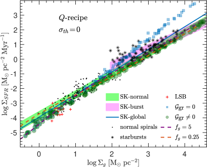
Figure 1: The star formation rate per unit area versus the gas surface density for 100 sets of random parameters generated as described in the text. Blue squares are obtained with only SN feedback, while the green circles also include gravitational heating. The dashed lines illustrate the dependence on the ratio $f_{g}=\Sigma_{g}/\Sigma_{\ast}$. Green and pink shaded areas represent the SK laws inferred, respectively, from observations of normal spirals (De Los Reyes & Kennicutt, 2019) and starbursts (Kennicutt & De Los Reyes, 2021). Their widths corresponds the rms intrinsic scatter around the inferred law. Black dots and asterisks show the actual measurements of normal spirals and starbursts. Red plus sign symbols show the LSB galaxy sample of (Wyder et al., 2009). The top panel and bottom panels correspond to the $Q$- and $\rho$-recipe as indicated in the figure. For comparison, the solid blue line is a global SK fit to the normal and starburst galaxies, with $n=1.54$. The bottom panel is the same as the top but for the $\rho$-recipe. There is a marked deviation of the blue points at $\Sigma_{g}\approx\,\Sigma_{g}^{\textrm{thr}}=50\,{\rm M}_{\odot}\,{\rm pc}^{-2}$.

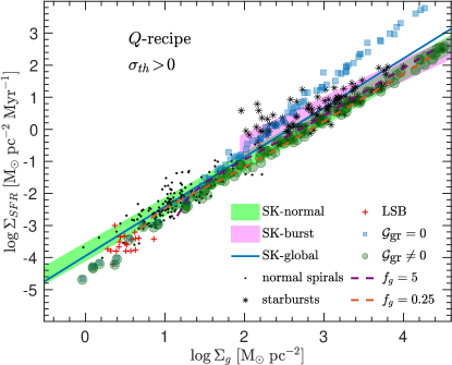
Figure 2: The same as the previous figure, but with a non-vanishing thermal floor in the velocity dispersion.

Appendix B presents further analyses and numerical investigation in terms of the depletion time scale, $t_{{}_{SF}}/\epsilon_{{}_{SF}}$, and the gain and loss terms.

7.2 Velocity dispersion and Toomre parameter

As emphasized by Krumholz et al. (2018), models should be able to recover the observed $\sigma_{g}$ in relation to the SFR. Krumholz et al. (2018) explore their model prediction for $\sigma_{g}$ versus the total star formation rate, $\dot{M}_{*}$ (total mass in stars formed per unit time). Their detailed mass transport model allows them to integrate $\Sigma_{SFR}$ to obtain $\dot{M}_{*}$. In principle, we can augment our model with assumptions regarding the size of the disk in order to estimate $\dot{M}_{*}$. However, we opt to restrict the analysis to the more robust model prediction for the correlation of $\sigma_{g}$ versus $\Sigma_{SFR}$. The results are presented in Fig. 3 for the sets of random parameters, as the green circles (including gravitational and SN heating) and blue squares (including only SN heating) in the $Q$-recipe. Dashed curves correspond to two specific values for $f_{g}$, as in Fig. 1. The figure shows the turbulent component of the velocity dispersion, which should be added in quadrature to $\sigma_{th}$ to find $\sigma_{g}$. Similar results are obtained for the $\rho$-recipe and hence, for brevity, we show only the $Q$-recipe.

The difference between the predictions with and without gravitational heating is pronounced at high $\Sigma_{SFR}$. As seen by the blue points in the figure, SN heating alone leads to a nearly constant $\sigma_{t}$ over the whole plotted range of six orders of magnitude in $\Sigma_{SFR}$. Gravitational heating boosts $\sigma_{t}$ at high $\Sigma_{SFR}$, as indicated by the rise of the green circles for $\Sigma_{SFR}\mathrel{\hbox to0.0pt{\lower 4.0pt\hbox{\hskip 0.5pt$\sim$}\hss}\raise 1.0pt\hbox{$>$}}10^{-2}\,{\rm M}_{\odot}\,{\rm pc}^{-2}\,\textrm{Myr}^{-1}$ (corresponding to $\Sigma_{g}\mathrel{\hbox to0.0pt{\lower 4.0pt\hbox{\hskip 0.5pt$\sim$}\hss}\raise 1.0pt\hbox{$>$}}\,\Sigma_{g}^{\textrm{thr}}$).

Swinbank et al. (2012) present measurements of $\sigma_{g}$ versus $\Sigma_{SFR}$ in a sample of nine star-forming galaxies at redshifts $z=0.8-2.2$. They derive the velocity dispersion from star forming clumps in the SHiZEL galaxies. These authors also find that these galaxies follow an SK law with parameters consistent with the local relation. Therefore, a comparison of their measurements with the results obtained here is appropriate. The data points are shown as the red crosses in the figure with the bars representing the errors provided in Swinbank et al. (2012). Although, the data points lie somewhat above the theoretical predictions for the gravitational heating case, the overall agreement is encouraging. The velocity dispersion obtained with SN heating alone, is markedly below the observations.

Also plotted in the figure are data used in Krumholz et al. (2018) whenever the sizes of the star-forming regions are available. Once this information is available we estimate $\Sigma_{SFR}$. For the galaxies in $z\sim 2-3$ sample of (Law et al., 2009), the area of nebular emission is provided in their table 3. The corresponding data is shown as blue diamonds, where the horizontal error bars represent the uncertainties in the area only and not in the observed $\dot{M}_{\ast}$. The vertical error bars on $\sigma_{g}$ are taken from their table 5. For The HI Nearby Galaxy Survey (THINGS, Ianjamasimanana et al., 2012), we take $\dot{M}_{\ast}$ and $l_{SFR}$ from table 4 in Leroy et al. (2008) and estimate $\Sigma_{SFR}\approx 0.26\dot{M}_{\ast}/\pi l_{SFR}^{2}$ where the factor $0.26$ accounts for the fraction of SFR within the scale radius $l_{SFR}$ of their exponential fits to the radial SFR profiles. We have found by visual inspection that these estimates of the $\Sigma_{SFR}$ are a reasonable fit to the averages of the $\Sigma_{SFR}$ profiles plotted in the appendix of Leroy et al. (2008). For the sample of local dwarf galaxies of Stilp et al. (2013a), the values of $\Sigma_{SFR}$ are provided in their table 3. The relevant data for the WiggleZ ($z\sim 1.3$) galaxies are available in Wisnioski et al. (2011). We follow Krumholz et al. (2018) and estimate $\dot{M}_{\ast}$ from the H$\alpha$ luminosity using the relation in Kennicutt et al. (2012). We derive $\Sigma_{SFR}$ based on the half-light radius of H$\alpha$ emission given in table 4 of Wisnioski et al. (2011).

Although we do not have error bars available for all data points, there can be up to a factor of two ambiguity in the derivation of $\Sigma_{SFR}$. There is a good general agreement between the observations and the gravitational heating model predictions at $\Sigma_{SFR}\mathrel{\hbox to0.0pt{\lower 4.0pt\hbox{\hskip 0.5pt$\sim$}\hss}\raise 1.0pt\hbox{$>$}}10^{-3}\,\,{\rm M}_{\odot}\,{\rm pc}^{-2}\,{\rm Myr}^{-1}$. At lower values of $\Sigma_{SFR}$, the models with and without gravitational heating tend to underpredict the observed velocity dispersion, mainly the (Stilp et al., 2013a) sample of local dwarfs and low mass spirals. Note that only the turbulent component is plotted for the model prediction. The addition of a thermal component of $\sigma_{th}\sim 5\,{\rm km}\,{\rm s}^{-1}$ mitigates this discrepancy for some galaxies, but it is unlikely to explain the velocity dispersion of $\sim 10\,{\rm km}\,{\rm s}^{-1}$ (Stilp et al., 2013b). Therefore, as discussed in detail in Stilp et al. (2013b), it is unclear how to account for high velocity dispersion seen in some galaxies in their sample of local dwarfs and low mass spirals.

Related to the velocity dispersion is the Toomre parameter. This is plotted in Fig. 4 for $\sigma_{th}=0$ for the two star formation recipes. The results for $\sigma_{th}=5\,{\rm km}\,{\rm s}^{-1}$ are similar except that at low $\Sigma_{g}$ there are fewer in the $Q$-recipe, while slightly larger values are acquired by $Q$ in the $\rho$-recipe.

By construction, the stellar Toomre parameter, $Q_{s}$, remains above unity in both recipes. For the $Q$-recipe (top panel), the global $Q$ is always below unity since a stable disk ($Q>1$) neither forms stars nor allows for collapse of perturbations. Hence the heating terms vanish and no energy balance is possible for $Q>1$. There is a transition in the distribution of $Q$ as a function of $\Sigma_{g}$. Below $\Sigma_{g}\approx\,\Sigma_{g}^{\textrm{thr}}$, both $Q_{g}$ and $Q_{s}$ are generally above unity, while the $Q$ values are concentrated around unity with little scatter at $\Sigma_{g}\rightarrow 0$. This is consistent with the expression in Eq. 24 for $Q$ derived for low $\Sigma_{g}$.

Above $\,\Sigma_{g}^{\textrm{thr}}$, both $Q$ and $Q_{g}$ spread below unity reaching values as low as $0.3$. A detailed inspection of the results, reveals that points with low $Q$ are associated with high $\Sigma_{g}/\Sigma_{\ast}$ ratios, while $Q\approx 1$ are obtained for disks dominated by the stellar component.

The $\rho$-recipe (bottom panel) also shows a similar transition of $Q$ versus $\Sigma_{g}$ reflecting the importance of gravitational heating at $\Sigma_{g}\mathrel{\hbox to0.0pt{\lower 4.0pt\hbox{\hskip 0.5pt$\sim$}\hss}\raise 1.0pt\hbox{$>$}}\,\Sigma_{g}^{\textrm{thr}}$. At high $\Sigma_{g}$, the results are very similar to the $Q$-recipe since the energy input from star formation becomes subdominant and energy balance is possible only for unstable disks. At low $\Sigma_{g}$, star formation is possible for $Q>1$ in the $\rho$-recipe, as seen in the figure.

There are several observational estimates of the Toomre parameter in the literature. We emphasize that the value $Q=1$ marking the stability transition is obtained under limited conditions and should not strictly hold for realistic cases due to deviations from these assumptions and large observational uncertainties. Kennicutt (1989) and Martin & Kennicutt (2001) measure the Toomre parameter using the expression for a single fluid without including the stellar component and assuming the same velocity dispersion of $6\,{\rm km}\,{\rm s}^{-1}$ for all galaxies in their analysis. These measurements were consistent with the SFR related to a critical surface density defined by the Toomre parameter, but with large variations. Leroy et al. (2008) provide estimates of the Toomre parameters for THINGS galaxies assuming a fixed gas velocity dispersion of $11\,{\rm km}\,{\rm s}^{-1}$ and stellar velocity dispersion inferred from vertical hydrostatic equilibrium. These authors obtain $Q$, $Q_{s}$ and $Q_{g}$ values that are markedly above the stability regime advocated by Kennicutt (1989) and Martin & Kennicutt (2001) with a large scatter. They show that this is a reflection of different assumptions from Kennicutt (1989) and Martin & Kennicutt (2001) regarding the velocity dispersion and the conversion of CO emission into mass of molecular hydrogen. Therefore, we conclude that detailed comparisons of model $Q$ with observations are indecisive.

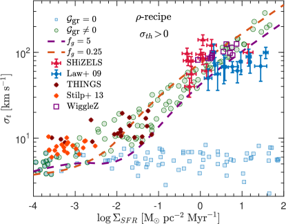
Figure 3: The turbulent component of the gas velocity dispersion, $\sigma_{t}$, versus $\Sigma_{SFR}$ for the $\rho$-recipe with a thermal velocity dispersion floor $\sigma_{th}=5\,{\rm km}\,{\rm s}^{-1}$. Circles and squares represent solutions of the energy balance equation with and without gravitational heating, while the red triangles correspond to data from (Swinbank et al., 2012). The dashed lines correspond to gas to $f_{\textrm{g}}=\Sigma_{g}/\Sigma_{\ast}=0.25$ and $5$, as indicated in the figure.

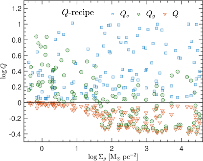
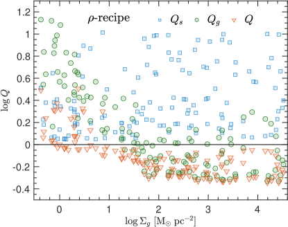
Figure 4: The global, stellar and gas Toomre parameters obtained in the two star formation recipes. Top and bottom panels are for the $Q$- and $\rho$-recipes, as indicated in the figure.

7.3 Scatter and Dependence on $\epsilon_{{}_{SF}}$ and $\eta$

The analysis so far referred to a single choice for the parameters $\epsilon_{{}_{SF}}$ and $\eta$. Many factors play a role in fixing these parameters, e.g. the details of the disk morphology, properties of star forming molecular gas, external tidal fields, and the DM distribution. Therefore, both of these parameters are likely to vary among galaxies and even across regions in the same galaxy. These variations can enhance the scatter in the predicted $\Sigma_{SFR}$.

We explore the dependence of the $\Sigma_{SFR}-\Sigma_{g}$ relation on $\epsilon_{{}_{SF}}$ and $\eta$ in Fig. 5. In both panels, we fix $\Omega=0.034\,{\rm km}\,{\rm s}^{-1}\;\textrm{pc}^{-1}$ and $V_{SN}=3000\,{\rm km}\,{\rm s}^{-1}$. The top panel refers to varying $\epsilon_{{}_{SF}}$, while fixing $\eta$ at the default values in each recipe (table 2). The $\Sigma_{SFR}$ curves in this panel correspond to $0.5\epsilon_{{}_{SF}}$ (amber) and $2\epsilon_{{}_{SF}}$ (purple) where here $\epsilon_{{}_{SF}}$ is the default value in each recipe. Similarly, the bottom panel probes the sensitivity to $\eta$ with $\epsilon_{{}_{SF}}$ fixed at the default values. In the two panels, we plot $\Sigma_{SFR}$ normalized by the curve obtained from the default values of $\eta$ and $\epsilon_{{}_{SF}}$.

There is a strong dependence on $\epsilon_{{}_{SF}}$ at $\Sigma_{g}\mathrel{\hbox to0.0pt{\lower 4.0pt\hbox{\hskip 0.5pt$\sim$}\hss}\raise 1.0pt\hbox{$>$}}\,\Sigma_{g}^{\textrm{thr}}$ in both recipes. At large $\Sigma_{g}$, SN heating becomes negligible and the velocity dispersion is mainly fixed by a balance between gravitational heating and dissipation. Therefore, $t_{{}_{SF}}$ is almost independent of $\epsilon_{{}_{SF}}$ and $\Sigma_{SFR}=\epsilon_{{}_{SF}}\Sigma_{g}/t_{{}_{SF}}$ varies linearly with $\epsilon_{{}_{SF}}$ in the limit of very large $\Sigma_{g}$ as seen in the top panel in the figure.

In the regime of $\Sigma_{g}~{}\hbox to0.0pt{$<$\hss}{\lower 4.30554pt\hbox{$\sim$}}\,\Sigma_{g}^{\textrm{thr}}$ where gravitational heating is subdominant, the dependence on $\epsilon_{{}_{SF}}$ is very weak for the $Q$-recipes. This interesting result can be understood as follows. Eq. 24, appropriate for this recipe in the low $\Sigma_{g}$ limit, implies

$$\omega_{1}=(217\textrm{Myr})^{-1}\left(\frac{\eta}{10}\right)\left(\frac{0.01}{\epsilon_{{}_{SF}}}\right)\left(\frac{3000}{V_{SN}}\right)\Sigma_{g}$$ (28)

where $\Sigma_{g}$ in $\,{\rm M}_{\odot}\,{\rm pc}^{-2}$, $V_{SN}$ in $\,{\rm km}\,{\rm s}^{-1}$ and we have used $\omega_{1}=\kappa(Q^{-2}-1)^{1/2}$. The result is independent of $\kappa$. Therefore,

$$\Sigma_{SFR} = \epsilon_{{}_{SF}}\Sigma_{g}\omega_{1}\approx\eta\frac{\pi G\Sigma_{g}^{2}}{V_{SN}}$$ (29)

$$= 4.5\times 10^{-5}\left(\frac{\eta}{10}\right)\left(\frac{3000}{V_{SN}}\right)\Sigma_{g}^{2}\;,$$ (30)

which is independent of both $\epsilon_{{}_{SF}}$ and $\kappa$. Although the quadratic dependence in this limit does not match the SK law on average, the scatter in the prediction due to varying $\Sigma_{g}/\Sigma_{\ast}$ is large at low $\Sigma_{g}$ as seen in Fig. 1.

In contrast, the figure shows that SFR in the $\rho$-recipe in the limit of $\Sigma_{g}\rightarrow 0$, is sensitive to to $\epsilon_{{}_{SF}}$ and implies that $\Sigma_{SFR}\sim\epsilon_{{}_{SF}}^{1/2}$. This is consistent with the following analytic considerations. The dissipation scale in this recipe is the disk height $H$ and the SF time scale if fixed by $1/\sqrt{G\rho}$. The vertical balance equation Eq. 10 can be used to relate these quantities to $\sigma$ in the energy balance equation Eq. 23. In the limit of very small $\Sigma_{g}$, only the halo gravity is relevant on the r.h.s of Eq. 10, giving $\rho\sigma_{g}=\Omega\Sigma_{g}/\sqrt{2\pi}$. Using this in the energy balance equation without the inclusion of the Toomre heating term, we arrive at

$$\sigma_{g}=(2\pi)^{1/4}\frac{\epsilon_{{}_{SF}}}{\eta}\frac{V_{SN}}{\Omega}\left(\Omega G\Sigma_{g}\right)^{1/2}\;.$$ (31)

After some algebra, we write the SFR in the low $\Sigma_{g}$ limit in the $\rho$-recipe as

$$\Sigma_{SFR}=(2\pi)^{-3/8}\left(\epsilon_{{}_{SF}}\eta\right)^{1/2}\!\left(\frac{G\Omega^{3}}{V_{SN}}\right)^{1/2}\!\Sigma_{g}^{3/2}\;.$$ (32)

Thus we $\Sigma_{SFR}\sim\epsilon_{{}_{SF}}^{1/2}$ as seen in the figure for small $\Sigma_{g}$.

The bottom panel of Fig. 5 explores the sensitivity on the dissipation parameter $\eta$. In the limit of small $\Sigma_{g}$, the dependence in both recipe is consistent with the expressions derived above, i.e. $\Sigma_{SFR}\sim\eta$ and $\eta^{1/2}$, respectively, for the $Q$- and $\rho$-recipes. At large $\Sigma_{g}$, energy balance between the dominant gravitational heating and dissipation determines $\sigma_{g}$ and thus, indirectly, $\Sigma_{SFR}$. The dependence can in principle be derived analytically in both recipes. For example, for an entirely gaseous disk in the $Q$-recipe, $\Sigma_{SFR}\sim\eta^{1/2}$ at large surface densities which does not fit behavior of the solid curves in the lower panel in Fig. 5 due to the small gas fraction ($f_{g}=0.25$) adopted in this figure.

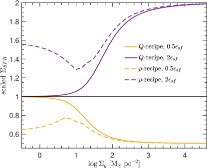
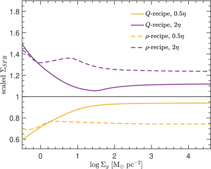
Figure 5: Dependence on the parameters $\epsilon_{{}_{SF}}$ (top) and $\eta$ (bottom). Solid and dashed lines refer, respectively, to the $Q$- and $\rho$-recipe. Purple and yellow colors, respectively, correspond to twice and one half the default values.

8 Porosity

Global self-regulation by SN feedback alone can be achieved if the fraction of volume, $f$, occupied by hot gas in percolating SN remnants is appreciable but also not too large (Silk, 1997, 2001; Li et al., 2015). The filing fraction is $f=1-\mathrm{e}^{-{\cal P}}$, where the porosity, ${\cal P}$, is the product of the SN rate (number per unit volume per unit time) times the 4-volume of an SN remnant at maximum extent. In an SN regulated disk, ${\cal P}\sim 1$; a disk with ${\cal P}\gg 1$ generates galactic fountains and winds and thus reducing the amount of gas available for star formation, while ${\cal P}\ll 1$ implies the disk gas is mostly cold, allowing the development of a surge of star formation until ${\cal P}\sim 1$ is reached. This however refers to the case where the heating term in the energy balance equation is dominated by star formation feedback. Gravitational heating operating mainly at high $\Sigma_{g}$, relaxes the condition of ${\cal P}\sim 1$ and can allow for a steady state with ${\cal P}\ll 1$ by countering dissipation.

The porosity expression derived by Silk (1997) can be re-cast in the following form

$${\cal P}=(G\rho_{g})^{-1/2}\frac{\Sigma_{SFR}}{\Sigma_{g}}\left(\frac{\sigma_{f}}{\sigma_{g}}\right)^{2.7}\;,$$ (33)

where $\sigma_{f}$ is a fiducial velocity dispersion that is proportional to $m_{*}^{-1}$. For $m_{*}=250\,\textrm{M}_{\odot}$, $\sigma_{f}=22\,{\rm km}\,{\rm s}^{-1}$. Despite its importance, estimation of porosity based on this expression is highly uncertain due to the steep dependence on $\sigma_{g}$ and $\sigma_{f}$. Taking $m_{*}=50\,\textrm{M}_{\odot}$ instead of $250\,\textrm{M}_{\odot}$, reduces the porosity estimation by a factor $\sim 80$ for the same $\Sigma_{SFR}$, $\sigma_{g}$ and $\rho_{g}$.

Nonetheless, it is prudent to confirm that the porosity in our model is reasonable. In Fig. 6, we plot the ${\cal P}$ obtained by applying the expression in Eq. 33 on our random sets of parameters where $\sigma_{g}$ is, as before, computed from the energy balance equation with and without gravitational heating. The figure refers to $\sigma_{th}=5\,{\rm km}\,{\rm s}^{-1}$ for the $\rho$-recipe only. For $\sigma_{th}=0$ the porosity would be limited by the turbulence velocity dispersion $\sigma_{t}$ alone. According to Fig. 3, $\sigma_{t}\sim 3\,{\rm km}\,{\rm s}^{-1}$ at low $\Sigma_{g}$, leading to very large ${\cal P}$ if $\sigma_{th}=0$. The $Q$-recipe leads to similar results except that there are fewer points at low $\Sigma_{g}$. The scatter of ${\cal P}$ for the same $\Sigma_{g}$ seen in the figure is almost entirely due to $m_{*}$ which is distributed randomly in the range $70-200\,\textrm{M}_{\odot}$. Smaller ${\cal P}$ values are associated with larger $m_{*}$.

For the $\mathcal{G}_{\textrm{gr}}=0$ case (blue squares), the porosity acquires reasonable values for all $\Sigma_{g}$, with a declining trend toward higher $\Sigma_{g}$. Although ${\cal P}\propto\Sigma_{SFR}/\Sigma_{g}\sim\Sigma_{g}^{0.5}$ for $\mathcal{G}_{\textrm{gr}}=0$, the mild increase in the velocity dispersion with $\Sigma_{g}$ (see Fig. 3) is sufficient to counter the term $\Sigma_{SFR}/\Sigma_{g}$.

The inclusion of gravitational heating has a dramatic effect on ${\cal P}$ at $\Sigma_{g}\mathrel{\hbox to0.0pt{\lower 4.0pt\hbox{\hskip 0.5pt$\sim$}\hss}\raise 1.0pt\hbox{$>$}}\,\Sigma_{g}^{\textrm{thr}}$ (green circles). The significant boost in $\sigma_{t}$ at $\Sigma_{g}\mathrel{\hbox to0.0pt{\lower 4.0pt\hbox{\hskip 0.5pt$\sim$}\hss}\raise 1.0pt\hbox{$>$}}\,{\rm M}_{\odot}\,{\rm pc}^{-2}$ due to gravito-turbulence (Fig. 3), and the steep dependence of ${\cal P}$ on $\sigma_{g}$, are the reason for the sharp drop in ${\cal P}$ at high $\Sigma_{g}$.

Porosity remains $\sim 1$ for the $\Sigma_{g}$ range appropriate for normal spirals. According to Fig. 1 starbursts with surface densities in the range $\Sigma_{g}\sim 100-300\,{\rm M}_{\odot}\,{\rm pc}^{-2}$ are curiously matched by the model with $\mathcal{G}_{\textrm{gr}}=0$ (blue squares) while the model including gravitational heating (green circles) underpredicts $\Sigma_{SFR}$. Therefore, it is possible that SN-feedback remains dominant for starbursts in this range of $\Sigma_{g}$. If this is the case then we expect ${\cal P}\sim 1$ in these starbursts. At higher densities, SN-feedback weakens relative to gravitational heating and we expect ${\cal P}\ll 1$ according to Fig. 6.

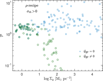
Figure 6: The porosity of the ISM versus $\Sigma_{g}$ in the $\rho$-recipe obtained using the expression in Eq. 33 where the velocity dispersion, $\sigma_{g}$, is obtained from the energy balance equation. Blue squares correspond to SN heating only ($\mathcal{G}_{\textrm{gr}}=0$), while the green circles are derived with gravitational heating switched on ($\mathcal{G}_{\textrm{gr}}\neq 0$) in addition to SN feedback.

9 comparison with the other models in the literature

Forbes et al. (2014) and Krumholz et al. (2018) distinguished between star formation in the GMC and the Toomre regimes. The time-scale in the former regime is fixed at a constant value of $2\rm Gyr$, while the latter is determined by the midplane gas density $\rho_{g}$ (which they express in terms of $Q$ and the angular velocity of the galaxy, among other parameters). The Toomre regime is adopted whenever the corresponding star formation time-scale if shorter than the fixed value of $2\rm Gyr$. The time-scale in their Toomre regime is actually the counterpart of our $\rho$-recipe. Our Fig. 3 implies that $\rho_{g}\sim(\Sigma_{g}/\sigma_{g})^{2}$ is an increasing function of $\Sigma_{g}$. Thus this regime is relevant to high $\Sigma_{g}$ galaxies. According to Eq. 50 in Krumholz et al. (2018), the rate (per unit area) of gravitational heating via transport is $\sim\sigma_{g}^{3}\Omega^{2}$ in the limit of high $\Sigma_{g}$, which is proportional to the heating rate implied in the $\rho-$recipe. Therefore, in this limit of $\Sigma_{g}$, we expect our model to yield similar scaling as the transport model by Krumholz et al. (2018). Indeed, the slopes of $\log\Sigma_{SFR}$ versus $\log\Sigma_{g}$ are similar as revealed by comparing Fig. 1 here with Figs. 2&3 in Krumholz et al. (2018). Further, the velocity dispersion derived in the two models are in the same range. Another similarity between the two models is that SN heating dominates at low $\Sigma_{g}$ below a threshold value ($\,\Sigma_{g}^{\textrm{thr}}$ in our model). In this limit, the dependence of $\Sigma_{SFR}$ on $\Sigma_{g}$ approaches $\Sigma_{g}^{2}$ and the velocity dispersion acquires $\sigma_{g}\sim 5-10\,{\rm km}\,{\rm s}^{-1}$ with weak dependence on $\Sigma_{g}$. This scaling can readily by derived by equating the weight of the disk by the vertical momentum injection by SN in the midplane (Ostriker & Shetty, 2011). However, we emphasize that even in the SN dominant limit, vertical balance alone is insufficient to yield $\sigma_{g}$ to close a self-regulating star formation versus feedback loop.

Bacchini et al. (2020) present a detailed analysis of the kinematic of ten nearby star forming galaxies. They find that SN feedback is sufficient to maintain the observed turbulence level. The gas surface density in these galaxies is lower than the threshold value obtained here, therefore, these findings are actually consistent with our model. However, we note that, in contrast us, their model of star formation induced turbulence is based on SN energy output rather than momentum injection into the ISM.

Star formation models based on the turbulence properties of MCs have been developed (e.g Krumholz & McKee, 2005; Padoan & Nordlund, 2011; Federrath & Klessen, 2012; Padoan et al., 2017; Burkhart, 2018). These models rely on an assumed (but simulation-motivated) form for the probability distribution of the gas density inside turbulent MCs, with star formation ensuing in sub-cloud regions with sufficiently high densities. These considerations can be used to provide the global star formation rate in the disk under certain conditions regarding marginally disk stability and the fraction of molecular gas. Turbulence within individual MCs plays an important role in their overall stability and establishing the distribution of density fluctuations inside them (Zuckerman & Evans, 1974; Fleck, 1980; Scalo & Elmegreen, 2004; Larson, 1981; Bonazzola et al., 1987; Falgarone & Phillips, 1990; Krumholz & McKee, 2005; Hennebelle & Chabrier, 2011; Federrath & Klessen, 2012; Mocz et al., 2017; Padoan et al., 2017). This turbulence can be triggered by global gravitational and MHD instability over large scales of 100s of parsecs. Further, at high SN rate and high gas surface densities, turbulence can be boosted by nearby SNs (e.g Ballesteros-Paredes et al., 2007; Seifried et al., 2018). Simulations demonstrate that gravito-turbulence within MCs is necessary to explain the Larson relations (Larson, 1981) between the observed internal velocity dispersion and sizes (Ibáñez-Mejía et al., 2016).

In the limit of SN dominated heating, porosity of SN remnants must be $\sim 1$ if self-regulated feedback is maintained Silk (1997). Together, with a requirement of a marginally stable disk for maintaining star formation, it is possible to derive closed forms for the velocity dispersion and star formation law. Our model here is in agreement with this picture at $\Sigma_{g}~{}\hbox to0.0pt{$<$\hss}{\lower 4.30554pt\hbox{$\sim$}}\,\Sigma_{g}^{\textrm{thr}}$, but deviates from it when gravitational heating is included.

10 Discussion

In this paper, we have highlighted the role of self-gravity induced turbulence as a mechanism for regulating star formation in order to bring down the SFR relative to models invoking only SN feedback. However, it is known that turbulence can have the opposite effect of triggering star formation (Elmegreen, 2002; Federrath et al., 2010). Convergent turbulent motions in the ISM lead to large scale agglomeration of dense and cool gas, facilitating the conditions for star formation. AGN outflows also provide potential triggers of gas-rich disk star formation when the interstellar medium pressure is transiently enhanced (Silk & Norman, 2009; Ishibashi et al., 2013; Dugan et al., 2014; Bieri et al., 2016; Zubovas & Bourne, 2017). We will address the possible role of AGN elsewhere.

Here we note that that reconciliation of gravity-driven turbulence with the possible quenching or triggering of star formation depends on the detailed statistical properties of the density and velocity distribution in galactic turbulence. As pointed out by Ostriker & Shetty (2011), moderate densities generated by converging flows are likely to be dispersed before they can collapse to form stars. Thus, only a small fraction of the gas in the densest regions would be available for star formation via this mode. We note here that this actually might help explain the low star formation efficiency on galactic scales using the arguments of Krumholz & McKee (2005), but for turbulence on large scales rather than in MCs.

Turbulent motions driven by Toomre gravitational instabilities occur on a relatively large scale. For a Toomre parameter $Q~{}\hbox to0.0pt{$<$\hss}{\lower 4.30554pt\hbox{$\sim$}}1$, the disk scale-height is close to the driving scale, and turbulence should be three-dimensional and dissipate on small scales through a downward cascade of energy (Elmegreen et al., 2003). We have not considered the possibility of a quasi-two-dimensional inverse cascade turbulence initiated on scales larger than the disk height. A quasi-two-dimensional turbulence could be driven by long spiral arms (Bournaud et al., 2010) and even become dominant if $Q>1$.

Brucy et al. (2020) use numerical simulations to study the suppression of star formation by gravito-turbulence. Their study illustrates the insufficiency of SN feedback alone to regulate star formation at high surface densities. In their simulations (of a cube of $1\,{\rm kpc}$ on the side) gravito-turbulence driving is introduced by numerically injecting energy in the system rather than self-consistently as the result of gravitational instability. They consider a disk of marginal instability with $Q\sim 1$, in contrast to our model where the Toomre parameter can actually be less than unity at large $\Sigma_{g}$.

We have focused on a possible route for SFR regulation based on the dynamical properties of disks on large scales. Nonetheless, there are several layers to the process of star formation, involving a wide range of physical properties. Star formation occurs exclusively in MCs with sizes of tens of parsecs and mean number densities of $\mathcal{O}(100)\;\textrm{cm}^{-3}$, but with large variations of up to $10^{5}\;\textrm{cm}^{-3}$. Inside MCs, stars preferentially form in the densest regions over physical scales below hundreds of au, where the details of the local equation of state, metallicity and photoionizing feedback play a fundamental role in determining the initial stellar mass function (e.g. Dale et al., 2005; Hennebelle et al., 2019). Furthermore, there is an intricate interface between the MCs and the interstellar (ISM) medium on large scales. Radiative, gravitational and MHD processes on large scales likely dictate the formation of the MCs and their subsequent properties (Ballesteros-Paredes et al., 2007).

The standard disk gravitational stability analysis assumes a fixed $\sigma_{g}$ in the perturbed equations without perturbing $\sigma_{g}$ itself. In principle, with the restrictions imposed by Eq. 23, a a full stability analysis should incorporate perturbations in $\sigma_{g}$. This will introduce additional (thermal) instabilities on small scales and also modify the stability criteria on intermediate scales (Nusser, 2005). However, this is a lengthy analysis that is not expected to have a significant effect on the results.

Galactic outflows launched by the cumulative effect of stellar and/or AGN feedback are ubiquitously observed (c.f. Rupke, 2018, for a review). They likely have a profound impact on the global properties of galaxies, such as the their baryonic content, the DM density distribution and the overall star formation history. The model presented here assumes that the disk relaxes to a quasi-stationary state dictated by vertical pressure and energy balance. This quasi-equilibrium state will be transiently disturbed by rapid episodes of galactic winds, but it is assumed to persist on in the long time average sense. This assumption is partially supported by numerical simulations (e.g Smith et al., 2018).

One of the interesting observations in star formation is the long depletion time for turning gas into stars. The depletion time-scale is $\sim 20-100$ times larger than any dynamical timescale in the system, i.e. the star formation efficiency or the fraction of gas that actually turn into stars per dynamical timescale is very small. We do not make an attempt at explaining this issue and rather represent the star formation efficiency as a tunable parameter. The explanation for the low efficiency is most likely related to the susceptibility of MCs to stellar feedback (winds and photoionization) even before massive stars explode into supernovae (Elmegreen, 2000; Inutsuka et al., 2015; Kruijssen et al., 2019; Chevance et al., 2020). Some compelling evidence for this is presented by Kruijssen et al. (2019) for the spiral galaxy NGC 300 (but, see also Koda et al., 2009). Nonetheless, we have found (see Eq. 29) that at low disk surface densities and for a high gas fraction, the SFR per unit area is independent of the efficiency parameter and is dictated by the parameter $V_{SN}$ related to the momentum injected by SN into the ISM. The SFR in this case is also reasonable, and hence under certain conditions, the long depletion time-scales could be related to large-scale feedback in the disk rather than within MCs.

According to the SK law, a typical galaxy depletes its gas content over a time-scale of $\Sigma_{g}/\Sigma_{SFR}\sim 6\Sigma_{g}^{-0.41}$ Gyr ($\Sigma_{g}$ in $M_{\odot}\textrm{pc}^{-2}$) Schmidt et al. (2016). Therefore, at least for high $\Sigma_{g}$, refilling of the disk gas content is inevitable. Since on average, all galaxies will consume their gas, it is unlikely that galaxy mergers can provide the required gas supply. This motivates direct accretion of gas from the intergalactic medium as the main replenishment mechanism (Bournaud & Elmegreen, 2009; Dekel et al., 2009; Conselice et al., 2012; Lofthouse et al., 2017). Feeding of warm galactic coronae is an intermediate phase with potentially observable consequences. The circumgalactic medium may indeed control the galactic baryon budget (Tumlinson et al., 2017). Transport of accreted gas to the central disk has been observed in some galaxies (Schmidt et al., 2016). Further, cosmological zoom-in simulations of Milky Way-like galaxies find that gas accretion replenishes the supply of gas for disk star formation. The angular momentum of the accreted gas is similar to that at the edge of the gaseous disk (Trapp et al., 2020). The model of Krumholz et al. (2018) builds on the gravitational energy released via the transport in a sheared disk as the main source of gravito-turbulence.

A robust prediction of the model is that disks of normal spirals above a threshold surface density $\Sigma_{g}\sim 50\,{\rm M}_{\odot}\,{\rm pc}^{-2}$, cannot be regulated by SN feedback if the observed SK law is to be recovered. Gravito-turbulence dominates these disks, leading to $\Sigma_{SFR}$ consistent with the observations. Below this threshold, the disks are marginally stable with $Q\approx 1$. At higher surface densities, only disks dominated by the stellar component have $Q\approx 1$. Disks above the threshold but having a low ratio $\Sigma_{\ast}/\Sigma_{g}$, are associated with $Q<1$.

The situation is different for starburst galaxies. Starbursts with $\Sigma_{g}\sim 100-300\,{\rm M}_{\odot}\,{\rm pc}^{-2}$ are associated with $\Sigma_{SFR}$ predicted by SN feedback alone. In fact, gravitational heating suppresses the predicted $\Sigma_{SFR}$ by about an order of magnitude relative to the observations of starbursts in this range of surface densities. However, at larger $\Sigma_{g}$, starbursts tend to fall back to the $\Sigma_{SFR}$ level predicted by gravitational heating and consistent with an extrapolation of the SK law inferred for normal galaxies ($\Sigma_{g}~{}\hbox to0.0pt{$<$\hss}{\lower 4.30554pt\hbox{$\sim$}}170\,{\rm M}_{\odot}\,{\rm pc}^{-2}$)

The results are only moderately sensitive to the dissipation parameter $\eta$. An application of the model on the random sets of disk parameters with $\eta=3.5$ instead of the default $\eta=4.5$ leads to meagre differences in the results (see also Fig. 5). Although, the sensitivity to $\epsilon_{{}_{SF}}$ is more pronounced over the range of surface densities we consider, there is no need for fine-tuning. Variations of $~{}\hbox to0.0pt{$<$\hss}{\lower 4.30554pt\hbox{$\sim$}}\,20\%$ in $\epsilon_{{}_{SF}}$ yield reasonable matches to the star formation law, even with $\eta$ fixed to the default value.

11 acknowledgements

This research is supported by a grant from the Israeli Science Foundation grant number 936/18.

12 Data availability

No new data were generated or analysed in support of this research.

Appendix A approximate expressions, scale of least stable mode and disk height

We present tests of the approximate relations in Eqs. 5–7 for gravitational instability in a composite two-fluid disk. Fig. 7 presents such a comparison for a composite disk with $\kappa=0.035\,{\rm km}\,{\rm s}^{-1}\,\textrm{pc}^{-1}$, $\Sigma_{g}=15\,{\rm M}_{\odot}\,{\rm pc}^{-2}$ and $\Sigma_{\ast}=30\,{\rm M}_{\odot}\,{\rm pc}^{-2}$. The quantities $\omega_{1}$, $k_{1}$ and $Q$ are computed for a range of $\sigma_{g}$ for two fixed values of the ratio $\sigma_{g}/\sigma_{\ast}$. In the top panel, we plot $|\omega_{1}^{2}|/\kappa^{2}$ versus $Q$ where the crosses and open circles, respectively, correspond to the approximation in Eq. 6 and the exact result obtained from the exact relations in Jog & Solomon (1984). Only at $Q\approx 1$ for $\sigma_{g}/\sigma_{\ast}=0.3$, is there a significant difference between the approximate and exact results, but this is irrelevant in practice since $\omega_{1}\approx 0$ at this $Q$. Since the dependence on $\kappa$ and $Q$ in Eq. 6 is exact in linear theory, the plot essentially tests the validity of the Romeo & Wiegert (2011) approximation in Eq. 4 for $Q$. Although this approximation has been tested previously by these authors, we bring this comparison here simply to emphasize that it is also suitable for estimating $\omega_{1}$. The bottom panel of the same figure, shows $k_{1}$ in units of $\kappa/c_{s}$. Here also, the agreement between the approximate expression in Eq. 7 and the exact result based on Jog & Solomon (1984) is excellent.

In Fig. 8 we plot the scale ratios $H/H_{0}$ (Eq. 12) and $(Hk_{1})^{-1}$ versus the Toomre parameter, $Q$. The curves correspond to two values of $f_{\textrm{g}}=\Sigma_{g}/\Sigma_{\ast}$ as indicated in the figure. For each $f_{\textrm{g}}$, the ratio of the velocity dispersion $\sigma_{g}/\sigma_{\ast}$ is varied to produce the corresponding curve. We choose $\sigma_{\ast}$ such that $\sigma_{g}/\sigma_{\ast}=1$ yields $Q=1$ and hence all points with $Q>1$ ($Q<1$) have $\sigma_{g}/\sigma_{\ast}>1$ ($\sigma_{g}/\sigma_{\ast}<1$). As for the DM halo, we take $v_{\textrm{h}}=100\,{\rm km}\,{\rm s}^{-1}$ at $R=3\;\textrm{kpc}$. Deviation of $H/H_{0}$ from unity is an indication of the halo gravity on the disk height. The figure demonstrates that for unstable disks ($Q~{}\hbox to0.0pt{$<$\hss}{\lower 4.30554pt\hbox{$\sim$}}1$), halo gravity has a minor effect on the disk height. Further, we see that $1/k_{1}\sim H$ as long as $Q~{}\hbox to0.0pt{$<$\hss}{\lower 4.30554pt\hbox{$\sim$}}1$ and even larger $Q$ for a gas dominated disk as indicated by the solid red curve corresponding to $f_{g}=5$.

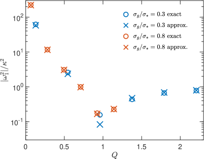
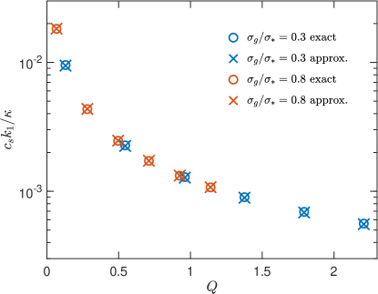
Figure 7: Top: accuracy of the approximate expression in Eq. 6 for $\omega_{1}$ as a function of the Toomre parameter $Q$ in a two fluid system with fixed $\kappa$, $\Sigma_{\ast}$ and $\Sigma_{g}$ (see text), for two values of $\sigma_{g}/\sigma_{\ast}$, as indicated in the figure. Bottom: test of the expression in Eq. 7 for the wavenumber $k_{1}$ of the least stable mode.

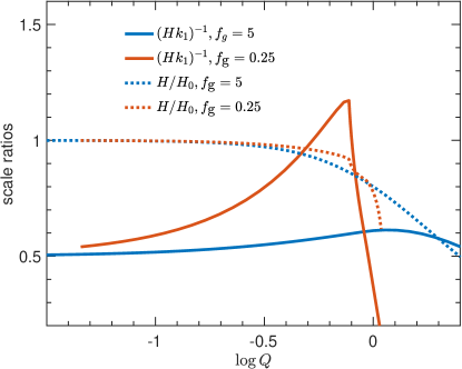
Figure 8: The solid curves show the ratio of $1/k_{1}$ to the disk scale height (including halo gravity), $H$. The dotted curves are $H/H_{0}$ where $H_{0}$ is computed for zero halo gravity. Results are plotted for two values of $f_{g}$, as indicated in the figure.

Appendix B depletion time, gain and loss terms

Fig. 9 examines in more details the differences in $Q$- and $\rho$-recipes by plotted the depletion timescale $\tau_{dep}=t_{{}_{SF}}/\epsilon_{{}_{SF}}$ for points shown in the previous figure. The main difference is at the low $\Sigma_{g}$ where the ratio is on average lower in the $\rho$-recipe. At larger $\Sigma_{g}$, the two recipes are essentially equivalent. This is in accordance with Eq. 15 and Fig. 8 showing that $k_{1}\sim H^{-1}$.

Leroy et al. (2017) and Querejeta et al. (2019) analyzed the star formation in the spiral galaxy M51. They find a mild anti-correlation between the molecular gas depletion time and the molecular gas surface density on the cloud scale. Our depletion times are in the same ballpark for the same range of $\Sigma_{g}$ in Fig. 9, but we find a stronger anti-correlation. Although most of the gas mass within $10\,{\rm kpc}$ in M51 is molecular (Scoville & Young, 1983), the surface density in our work is to be understood as an average over larger scales, rather than the individual molecular cloud scale. The reason is that disk stability addressed here depends on the average surface density rather than local densities of the clouds.

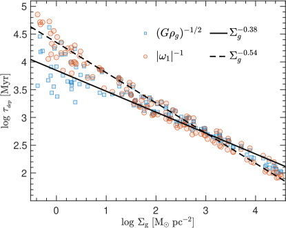
Figure 9: The gas depletion timescale $\tau_{dep}=\Sigma_{g}/\Sigma_{SFR}=t_{{}_{SF}}/\epsilon_{{}_{SF}}$ for $\sigma_{th}=0$.

We turn now to a direct comparison between the SN and gravitational heating terms, $\mathcal{G}_{\textrm{SN}}$ and $\mathcal{G}_{\textrm{gr}}$. Qualitatively, the picture is similar in both recipes and thus we present results only for the $Q$-recipe. The blue squares and amber circles in Fig. 10 represent, respectively, $\mathcal{G}_{\textrm{SN}}$ and $\mathcal{G}_{\textrm{gr}}$, obtained with $\sigma_{th}=0$ in the $Q$-recipe with the default parameter values. The points correspond to the top panel in Fig. 1. As inferred previously from Fig. 1, $\mathcal{G}_{\textrm{gr}}$ becomes more significant only at $\Sigma_{g}>10\,\,{\rm M}_{\odot}\,{\rm pc}^{-2}$.

Eq. 24 allows us to derive the dependence of the heating terms at low surface densities. Since $\mathcal{G}_{\textrm{gr}}=\omega_{1}\sigma_{{}_{\!Q=1}}^{2}$, the equation implies $\mathcal{G}_{\textrm{gr}}\sim\Sigma_{g}^{2}(Q^{-2}-1)^{1/2}\kappa^{-1}\sim\Sigma_{g}^{3}$ if the disk is purely gaseous and the contribution from $\Sigma_{g}$ to $\kappa$ is negligible. This is steeper than the slope of the linear regression line (dashed) of $\log\mathcal{G}_{\textrm{gr}}$ on $\Sigma_{g}$, obtained for the amber circles restricted to $\log\Sigma_{g}<1$. This is reasonable given our assumptions and the large scatter of the amber circles representing $\mathcal{G}_{\textrm{gr}}$ in the figure. We have checked that in fact linear regression yields a slope very close to $3$ when limited to points in a narrow range of $\kappa$ and $f_{\textrm{g}}$. Similar considerations imply $\mathcal{G}_{\textrm{SN}}\sim\Sigma_{g}^{2}$ which is steeper than the slope of the dotted line but, as before, this is due to the spread in $\kappa$ and $f_{\textrm{g}}$.

At large $\Sigma_{g}$, the epicyclic frequency is mainly fixed by $\Sigma_{g}$, i.e. $\kappa\sim\Sigma_{g}^{-1/2}$. Considering only the gravitational heating term in a gas-only disk, energy balance yields a Toomre parameter which depends just on $\eta$, i.e. $Q=Q(\eta)$ and hence $\mathcal{G}_{\textrm{gr}}\sim\kappa Q(\eta)\Sigma_{g}^{2}\sim\Sigma_{g}^{1.5}$, close to the slope of the dot-dashed line in Fig. 10. Further, $\sigma_{g}\sim Q(\eta)/\kappa\Sigma_{g}$ and hence $\mathcal{G}_{\textrm{SN}}\sim\kappa[Q(\eta)^{-2}-1)^{-1/2}\sigma_{g}\sim\Sigma_{g}$ in excellent agreement with the slope of the solid line.

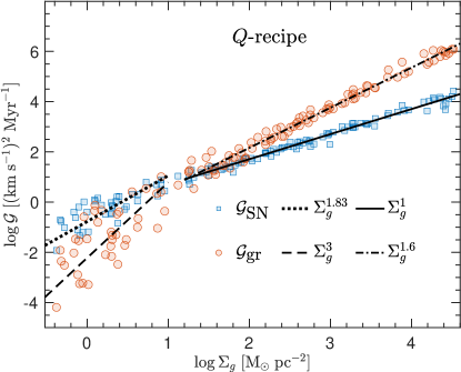
Figure 10: The energy injection rates (per unit mass) due to SN and gravitational heating, as indicated in the legend. $\sigma_{th}=0$

References

- Bacchini et al. (2020) Bacchini C., Fraternali F., Iorio G., Pezzulli G., Marasco A., Nipoti C., 2020, A&A, 641, A70
- Balbus & Cowie (1985) Balbus S. A., Cowie L. L., 1985, ApJ, 297, 61
- Balbus & Hawley (1998) Balbus S. A., Hawley J. F., 1998, Reviews of Modern Physics, 70, 1
- Ballesteros-Paredes et al. (2007) Ballesteros-Paredes J., Klessen R. S., Mac Low M. M., Vazquez-Semadeni E., 2007, in Protostars and Planets V, B. Reipurth, D. Jewitt, and K. Keil (eds.), University of Arizona Press, Tucson. p. 63, http://arxiv.org/abs/astro-ph/0603357
- Beck (2016) Beck R., 2016, AAR, 24, 4
- Benítez-Llambay et al. (2018) Benítez-Llambay A., Navarro J. F., Frenk C. S., Ludlow A. D., 2018, MNRAS, 473, 1019
- Bertin & Lodato (2001) Bertin G., Lodato G., 2001, A&A, 370, 342
- Béthune et al. (2021) Béthune W., Latter H., Kley W., 2021, A&A
- Bieri et al. (2016) Bieri R., Dubois Y., Silk J., Mamon G. A., Gaibler V., 2016, MNRAS, 455, 4166
- Bigiel et al. (2010) Bigiel F., Walter F., Blitz L., Brinks E., de Blok W. J. G., Madore B., 2010, The Astronomical Journal, 140, 1194
- Bonazzola et al. (1987) Bonazzola S., Heyvaerts J., Falgarone E., Perault M., Puget J. L., 1987, A&A, 172, 293
- Booth & Clarke (2019) Booth R. A., Clarke C. J., 2019, MNRAS, 483, 3718
- Bournaud & Elmegreen (2009) Bournaud F., Elmegreen B. G., 2009, ApJ, 694, 158
- Bournaud et al. (2010) Bournaud F., Elmegreen B. G., Teyssier R., Block D. L., Puerari I., 2010, MNRAS, 409, 1088
- Brucy et al. (2020) Brucy N., Hennebelle P., Bournaud F., Colling C., 2020, ApJL, 896, L34
- Burkhart (2018) Burkhart B., 2018, ApJ, 863, 118
- Chevance et al. (2020) Chevance M., et al., 2020, MNRAS, 000, 1
- Cioffi et al. (1988) Cioffi D. F., McKee C. F., Bertschinger E., 1988, ApJ, 334, 252
- Combes et al. (2012) Combes F., et al., 2012, A&A, 539, A67
- Conselice et al. (2012) Conselice C. J., Mortlock A., Bluck A. F. L., Gruetzbauch R., Duncan K., 2012, MNRAS, 430, 1051
- Crosthwaite et al. (2000) Crosthwaite L. P., Turner J. L., Ho P. T. P., 2000, AJ, 119, 1720
- Dale et al. (2005) Dale J. E., Bonnell I. A., Clarke C. J., Bate M. R., 2005, MNRAS, 358, 291
- De Los Reyes & Kennicutt (2019) De Los Reyes M. A., Kennicutt R. C., 2019, ApJ, 872, 16
- Dekel et al. (2009) Dekel A., et al., 2009, Nature, 457, 451
- Dugan et al. (2014) Dugan Z., Bryan S., Gaibler V., Silk J., Haas M., 2014, ApJ, 796, 113
- Efstathiou (2000) Efstathiou G., 2000, MNRAS, 317, 697
- Elmegreen (1989) Elmegreen B. G., 1989, ApJ, 338, 178
- Elmegreen (2000) Elmegreen B. G., 2000, ApJ, 530, 277
- Elmegreen (2002) Elmegreen B. G., 2002, ApJ, 577, 206
- Elmegreen & Elmegreen (1983) Elmegreen B. G., Elmegreen D. M., 1983, MNRAS, 203, 31
- Elmegreen et al. (2003) Elmegreen B. G., Elmegreen D. M., Leitner S. N., 2003, ApJ, 590, 271
- Falgarone & Phillips (1990) Falgarone E., Phillips T. G., 1990, ApJ, 359, 344
- Federrath & Klessen (2012) Federrath C., Klessen R. S., 2012, ApJ, 761, 156
- Federrath et al. (2009) Federrath C., Duval J., Klessen R. S., Schmidt W., Mac Low M. M., 2009, Proceedings of the International Astronomical Union, 5, 404
- Federrath et al. (2010) Federrath C., Roman-Duval J., Klessen R. S., Schmidt W., Low M.-M. M., 2010, A&A, 512, A81
- Fleck (1980) Fleck R. C., 1980, ApJ, 242, 1019
- Forbes et al. (2014) Forbes J. C., Krumholz M. R., Burkert A., Dekel A., 2014, MNRAS, 438, 1552
- Fuchs & Von Linden (1998) Fuchs B., Von Linden S., 1998, MNRAS, 294, 513
- Goldreich & Lynden-Bell (1965) Goldreich P., Lynden-Bell D., 1965, MNRAS, 130, 97
- Gurvich et al. (2020) Gurvich A. B., et al., 2020, MNRAS, 498, 3664
- Hennebelle & Chabrier (2011) Hennebelle P., Chabrier G., 2011, ApJL, 743, 29
- Hennebelle et al. (2019) Hennebelle P., Lee Y. N., Chabrier G., 2019, ApJ, 883, 140
- Hopkins et al. (2011) Hopkins P. F., Quataert E., Murray N., 2011, MNRAS, 417, 950
- Ianjamasimanana et al. (2012) Ianjamasimanana R., De Blok W. J., Walter F., Heald G. H., 2012, AJ, 144, 96
- Ibáñez-Mejía et al. (2016) Ibáñez-Mejía J. C., Mac Low M.-M., Klessen R. S., Baczynski C., 2016, ApJ, 824, 41
- Inoue et al. (2016) Inoue S., Dekel A., Mandelker N., Ceverino D., Bournaud F., Primack J., 2016, MNRAS, 456, 2052
- Inutsuka et al. (2015) Inutsuka S. I., Inoue T., Iwasaki K., Hosokawa T., 2015, A&A, 580, 49
- Ishibashi et al. (2013) Ishibashi W., Fabian A. C., Canning R. E., 2013, MNRAS, 431, 2350
- Jog & Solomon (1984) Jog C. J., Solomon P. M., 1984, ApJ, 276, 114
- Joung & Mac Low (2006) Joung M. K. R., Mac Low M.-M., 2006, ApJ, 653, 1266
- Julian & Toomre (1966) Julian W. H., Toomre A., 1966, ApJ, 146, 810
- Keller et al. (2014) Keller B. W., Wadsley J., Benincasa S. M., Couchman H. M., 2014, MNRAS, 442, 3013
- Kelly (2007) Kelly B. C., 2007, ApJ, 665, 1489
- Kennicutt (1989) Kennicutt R. C., 1989, ApJ, 344, 685
- Kennicutt (1998) Kennicutt R. C., 1998, ApJ, 498, 541
- Kennicutt & De Los Reyes (2021) Kennicutt R. C., De Los Reyes M. A. C., 2021, ApJ, 908, 61
- Kennicutt et al. (2012) Kennicutt R. C., Evans N. J., Kennicutt R. C., Evans N. J., 2012, ARA&A, 50, 531
- Kim & Ostriker (2015) Kim C. G., Ostriker E. C., 2015, ApJ, 802, 99
- Kim et al. (2016) Kim C.-G., Ostriker E. C., Raileanu R., 2016, ApJ, 834, 25
- Kim et al. (2020a) Kim W.-T., Kim C.-G., Ostriker E. C., 2020a, ApJ, 898, 35
- Kim et al. (2020b) Kim C.-G., et al., 2020b, ApJ, 900, 61
- Koda et al. (2009) Koda J., et al., 2009, ApJ, 700, 132
- Kruijssen et al. (2019) Kruijssen J. M. D., et al., 2019, Nature, 569, 519
- Krumholz & Burkhart (2016) Krumholz M. R., Burkhart B., 2016, MNRAS, 458, 1671
- Krumholz & McKee (2005) Krumholz M. R., McKee C. F., 2005, ApJ, 630, 250
- Krumholz et al. (2018) Krumholz M. R., Burkhart B., Forbes J. C., Crocker R. M., 2018, MNRAS, 477, 2716
- Larson (1981) Larson R. B., 1981, MNRAS, 194, 809
- Law et al. (2009) Law D. R., Steidel C. C., Erb D. K., Larkin J. E., Pettini M., Shapley A. E., Wright S. A., 2009, ApJ, 697, 2057
- Leroy et al. (2008) Leroy A. K., Walter F., Brinks E., Bigiel F., De Blok W. J., Madore B., Thornley M. D., 2008, AJ, 136, 2782
- Leroy et al. (2017) Leroy A. K., et al., 2017, ApJ, 846, 71
- Li et al. (2015) Li M., Ostriker J. P., Cen R., Bryan G. L., Naab T., 2015, ApJ, 814, 4
- Lin & Pringle (1987) Lin D. N. G., Pringle J. E., 1987, MNRAS, 225, 607
- Lofthouse et al. (2017) Lofthouse E. K., Kaviraj S., Conselice C. J., Mortlock A., Hartley W., 2017, MNRAS, 465, 2895
- Lovelace & Hohlfeld (1978) Lovelace R. V. E., Hohlfeld R. G., 1978, ApJ, 221, 51
- Lovelace & Hohlfeld (2013) Lovelace R. V. E., Hohlfeld R. G., 2013, MNRAS, 429, 529
- Lucas et al. (2020) Lucas W. E., Bonnell I. A., Dale J. E., 2020, MNRAS, 493, 4700
- Lynden-Bell (1966) Lynden-Bell D., 1966, Observatory, 86
- Mac Low & McCray (1988) Mac Low M.-M., McCray R., 1988, ApJ, 324, 776
- Martin & Kennicutt (2001) Martin C. L., Kennicutt Jr. R. C., 2001, ApJ, 555, 301
- Martizzi et al. (2015) Martizzi D., Faucher-giguère C. A., Quataert E., 2015, MNRAS, 450, 504
- McKee et al. (2015) McKee C. F., Parravano A., Hollenbach D. J., 2015, ApJ, 814, 13
- Mocz et al. (2017) Mocz P., et al., 2017, ApJ, 838, 40
- Nandakumar & Dutta (2020) Nandakumar M., Dutta P., 2020, MNRAS, 496, 1803
- Nusser (2005) Nusser A., 2005, MNRAS, 361, 977
- Ostriker & Shetty (2011) Ostriker E. C., Shetty R., 2011, ApJ, 731, 41
- Padoan & Nordlund (2011) Padoan P., Nordlund A., 2011, ApJ, 730, 40
- Padoan et al. (2017) Padoan P., Haugbølle T., Nordlund ., Frimann S., 2017, ApJ, 840, 48
- Querejeta et al. (2019) Querejeta M., et al., 2019, A&A, 625, A19
- Romeo & Falstad (2013) Romeo A. B., Falstad N., 2013, MNRAS, 433, 1389
- Romeo & Wiegert (2011) Romeo A. B., Wiegert J., 2011, MNRAS, 416, 1191
- Romeo et al. (2010) Romeo A. B., Burkert A., Agertz O., 2010, MNRAS, 407, 1223
- Rupke (2018) Rupke D. S., 2018, A review of recent observations of galactic winds driven by star formation, doi:10.3390/galaxies6040138, www.mdpi.com/journal/galaxies
- Scalo & Elmegreen (2004) Scalo J., Elmegreen B. G., 2004, ARAA, 42, 275
- Schmidt (1959) Schmidt M., 1959, ApJ, 129, 243
- Schmidt et al. (2016) Schmidt T. M., Bigiel F., Klessen R. S., de Blok W. J., 2016, MNRAS, 457, 2642
- Scoville & Young (1983) Scoville N., Young J. S., 1983, ApJ, 265, 148
- Seifried et al. (2018) Seifried D., Walch S., Haid S., Girichidis P., Naab T., 2018, ApJ, 855, 81
- Semelin & Combes (2000) Semelin B., Combes F., 2000, A&A, 360, 1096
- Silk (1997) Silk J., 1997, ApJ, 481, 703
- Silk (2001) Silk J., 2001, MNRAS, 324, 313
- Silk & Norman (2009) Silk J., Norman C., 2009, ApJ, 700, 262
- Smith et al. (2018) Smith M. C., Sijacki D., Shen S., 2018, MNRAS, 478, 302
- Stilp et al. (2013a) Stilp A. M., et al., 2013a, ApJ, 765, 136
- Stilp et al. (2013b) Stilp A. M., Dalcanton J. J., Skillman E., Warren S. R., Ott J., Koribalski B., 2013b, ApJ, 773, 88
- Swinbank et al. (2012) Swinbank A. M., Smail I., Sobral D., Theuns T., Best P. N., Geach J. E., 2012, ApJ, 760, 130
- Toomre (1964) Toomre A., 1964, ApJ, 139, 1217
- Trapp et al. (2020) Trapp C. W., et al., 2020, ArXiv:21015.11472, 1015.11472
- Tumlinson et al. (2017) Tumlinson J., Peeples M. S., Werk J. K., 2017, ANNU REV ASTRON ASTR, 55, 389
- Umurhan (2010) Umurhan O. M., 2010, A&A, 521, 25
- Wang & Silk (1994) Wang B., Silk J., 1994, ApJ, 427, 759
- Wentzel (1971) Wentzel D. G., 1971, ApJ, 163, 503
- Wisnioski et al. (2011) Wisnioski E., et al., 2011, MNRAS, 417, 2601
- Wyder et al. (2009) Wyder T. K., et al., 2009, AJ, 696, 1834
- Yu et al. (2021) Yu X., Bian F., Krumholz M. R., Shi Y., Li S., Chen J., 2021, MNRAS, 000, 1
- Zubovas & Bourne (2017) Zubovas K., Bourne M. A., 2017, MNRAS, 468, 4956
- Zuckerman & Evans (1974) Zuckerman B., Evans N. J. I., 1974, ApJ, 192, L149