NeRV: Neural Representations for Videos

Abstract

We propose a novel neural representation for videos (NeRV) which encodes videos in neural networks. Unlike conventional representations that treat videos as frame sequences, we represent videos as neural networks taking frame index as input. Given a frame index, NeRV outputs the corresponding RGB image. Video encoding in NeRV is simply fitting a neural network to video frames and decoding process is a simple feedforward operation. As an image-wise implicit representation, NeRV output the whole image and shows great efficiency compared to pixel-wise implicit representation, improving the encoding speed by 25$\times$ to 70$\times$, the decoding speed by 38$\times$ to 132$\times$, while achieving better video quality. With such a representation, we can treat videos as neural networks, simplifying several video-related tasks. For example, conventional video compression methods are restricted by a long and complex pipeline, specifically designed for the task. In contrast, with NeRV, we can use any neural network compression method as a proxy for video compression, and achieve comparable performance to traditional frame-based video compression approaches (H.264, HEVC etc.). Besides compression, we demonstrate the generalization of NeRV for video denoising. The source code and pre-trained model can be found at https://github.com/haochen-rye/NeRV.git.

1 Introduction

What is a video? Typically, a video captures a dynamic visual scene using a sequence of frames. A schematic interpretation of this is a curve in 2D space, where each point can be characterized with a $(x,y)$ pair representing the spatial state. If we have a model for all $(x,y)$ pairs, then, given any $x$, we can easily find the corresponding $y$ state. Similarly, we can interpret a video as a recording of the visual world, where we can find a corresponding RGB state for every single timestamp. This leads to our main claim: can we represent a video as a function of time?

More formally, can we represent a video $V$ as $V=\{v_{t}\}^{T}_{t=1}$, where $v_{t}=f_{\theta}(t)$, i.e., a frame at timestamp $t$, is represented as a function $f$ parameterized by $\theta$. Given their remarkable representational capacity [1], we choose deep neural networks as the function in our work. Given these intuitions, we propose NeRV, a novel representation that represents videos as implicit functions and encodes them into neural networks. Specifically, with a fairly simple deep neural network design, NeRV can reconstruct the corresponding video frames with high quality, given the frame index. Once the video is encoded into a neural network, this network can be used as a proxy for video, where we can directly extract all video information from the representation. Therefore, unlike traditional video representations which treat videos as sequences of frames, shown in Figure 1 (a), our proposed NeRV considers a video as a unified neural network with all information embedded within its architecture and parameters, shown in Figure 1 (b).

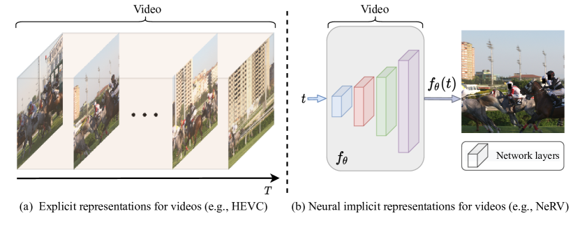
Figure 1: (a) Conventional video representation as frame sequences. (b) NeRV, representing video as neural networks, which consists of multiple convolutional layers, taking the normalized frame index as the input and output the corresponding RGB frame.

Table 1: Comparison of different video representations. Although explicit representations outperform implicit ones in encoding speed and compression ratio now, NeRV shows great advantage in decoding speed. And NeRV outperforms pixel-wise implicit representations in all metrics.

	Explicit (frame-based)		Implicit (unified)
	Hand-crafted (e.g., HEVC [2])	Learning-based (e.g., DVC [3])	Pixel-wise (e.g., NeRF [4]	Image-wise (Ours)
Encoding speed	Fast	Medium	Very slow	Slow
Decoding speed	Medium	Slow	Very slow	Fast
Compression ratio	Medium	High	Low	Medium

As an image-wise implicit representation, NeRV shares lots of similarities with pixel-wise implicit visual representations [5, 6] which takes spatial-temporal coordinates as inputs. The main differences between our work and image-wise implicit representation are the output space and architecture designs. Pixel-wise representations output the RGB value for each pixel, while NeRV outputs a whole image, demonstrated in Figure 2. Given a video with size of $T\times H\times W$, pixel-wise representations need to sample the video $T*H*W$ times while NeRV only need to sample $T$ times. Considering the huge pixel number, especially for high resolution videos, NeRV shows great advantage for both encoding time and decoding speed. Different output space also leads to different architecture designs, NeRV utilizes a MLP $+$ ConvNets architecture to output an image while pixel-wise representation uses a simple MLP to output the RGB value of the pixel. Sampling efficiency of NeRV also simplify the optimization problem, which leads to better reconstruction quality compared to pixel-wise representations.

We also demonstrate the flexibility of NeRV by exploring several applications it affords. Most notably, we examine the suitability of NeRV for video compression. Traditional video compression frameworks are quite involved, such as specifying key frames and inter frames, estimating the residual information, block-size the video frames, applying discrete cosine transform on the resulting image blocks and so on. Such a long pipeline makes the decoding process very complex as well. In contrast, given a neural network that encodes a video in NeRV, we can simply cast the video compression task as a model compression problem, and trivially leverage any well-established or cutting edge model compression algorithm to achieve good compression ratios. Specifically, we explore a three-step model compression pipeline: model pruning, model quantization, and weight encoding, and show the contributions of each step for the compression task. We conduct extensive experiments on popular video compression datasets, such as UVG [7], and show the applicability of model compression techniques on NeRV for video compression. We briefly compare different video representations in Table 1 and NeRV shows great advantage in decoding speed.

Besides video compression, we also explore other applications of the NeRV representation for the video denoising task. Since NeRV is a learnt implicit function, we can demonstrate its robustness to noise and perturbations. Given a noisy video as input, NeRV generates a high-quality denoised output, without any additional operation, and even outperforms conventional denoising methods.

The contribution of this paper can be summarized into four parts:

• We propose NeRV, a novel image-wise implicit representation for videos, representating a video as a neural network, converting video encoding to model fitting and video decoding as a simple feedforward operation.

• Compared to pixel-wise implicit representation, NeRV output the whole image and shows great efficiency, improving the encoding speed by 25$\times$ to 70$\times$, the decoding speed by 38$\times$ to 132$\times$, while achieving better video quality.

• NeRV allows us to convert the video compression problem to a model compression problem, allowing us to leverage standard model compression tools and reach comparable performance with conventional video compression methods, e.g., H.264 [8], and HEVC [2].

• As a general representation for videos, NeRV also shows promising results in other tasks, e.g., video denoising. Without any special denoisng design, NeRV outperforms traditional hand-crafted denoising algorithms (medium filter etc.) and ConvNets-based denoisng methods.

2 Related Work

Implicit Neural Representation. Implicit neural representation is a novel way to parameterize a variety of signals. The key idea is to represent an object as a function approximated via a neural network, which maps the coordinate to its corresponding value (e.g., pixel coordinate for an image and RGB value of the pixel). It has been widely applied in many 3D vision tasks, such as 3D shapes [9, 10], 3D scenes [11, 12, 13, 14], and appearance of the 3D structure [4, 15, 16]. Comparing to explicit 3D representations, such as voxel, point cloud, and mesh, the continuous implicit neural representation can compactly encode high-resolution signals in a memory-efficient way. Most recently, [17] demonstrated the feasibility of using implicit neural representation for image compression tasks. Although it is not yet competitive with the state-of-the-art compression methods, it shows promising and attractive proprieties. In previous methods, MLPs are often used to approximate the implicit neural representations, which take the spatial or spatio-temporal coordinate as the input and output the signals at that single point (e.g., RGB value, volume density). In contrast, our NeRV representation, trains a purposefully designed neural network composed of MLPs and convolution layers, and takes the frame index as input and directly outputs all the RGB values of that frame.

Video Compression. As a fundamental task of computer vision and image processing, visual data compression has been studied for several decades. Before the resurgence of deep networks, handcrafted image compression techniques, like JPEG [18] and JPEG2000 [19], were widely used. Building upon them, many traditional video compression algorithms, such as MPEG [20], H.264 [8], and HEVC [2], have achieved great success. These methods are generally based on transform coding like Discrete Cosine Transform (DCT) [21] or wavelet transform [22], which are well-engineered and tuned to be fast and efficient. More recently, deep learning-based visual compression approaches have been gaining popularity. For video compression, the most common practice is to utilize neural networks for certain components while using the traditional video compression pipeline. For example, [23] proposed an effective image compression approach and generalized it into video compression by adding interpolation loop modules. Similarly, [24] converted the video compression problem into an image interpolation problem and proposed an interpolation network, resulting in competitive compression quality. Furthermore, [25] generalized optical flow to scale-space flow to better model uncertainty in compression. Later, [26] employed a temporal hierarchical structure, and trained neural networks for most components including key frame compression, motion estimation, motions compression, and residual compression. However, all of these works still follow the overall pipeline of traditional compression, arguably limiting their capabilities.

Model Compression. The goal of model compression is to simplify an original model by reducing the number of parameters while maintaining its accuracy. Current research on model compression research can be divided into four groups: parameter pruning and quantization [27, 28, 29, 30, 31, 32]; low-rank factorization [33, 34, 35]; transferred and compact convolutional filters [36, 37, 38, 39]; and knowledge distillation [40, 41, 42, 43]. Our proposed NeRV enables us to reformulate the video compression problem into model compression, and utilize standard model compression techniques. Specifically, we use model pruning and quantization to reduce the model size without significantly deteriorating the performance.

3 Neural Representations for Videos

We first present the NeRV representation in Section 3.1, including the input embedding, the network architecture, and the loss objective. Then, we present model compression techniques on NeRV in Section 3.2 for video compression.

3.1 NeRV Architecture

Figure 2: (a) Pixel-wise implicit representation taking pixel coordinates as input and use a simple MLP to output pixel RGB value (b) NeRV: Image-wise implicit representation taking frame index as input and use a MLP $+$ ConvNets to output the whole image. (c) NeRV block architecture, upscale the feature map by $S$ here.

In NeRV, each video $V=\{v_{t}\}^{T}_{t=1}\in\mathbb{R}^{T\times H\times W\times 3}$ is represented by a function $f_{\theta}:\mathbb{R}\rightarrow\mathbb{R}^{H\times W\times 3}$, where the input is a frame index $t$ and the output is the corresponding RGB image $v_{t}\in\mathbb{R}^{H\times W\times 3}$. The encoding function is parameterized with a deep neural network $\theta$, $v_{t}=f_{\theta}(t)$. Therefore, video encoding is done by fitting a neural network $f_{\theta}$ to a given video, such that it can map each input timestamp to the corresponding RGB frame.

Input Embedding. Although deep neural networks can be used as universal function approximators [1], directly training the network $f_{\theta}$ with input timestamp $t$ results in poor results, which is also observed by [44, 4]. By mapping the inputs to a high embedding space, the neural network can better fit data with high-frequency variations. Specifically, in NeRV, we use Positional Encoding [4, 45, 6] as our embedding function

$$\Gamma(t)=\left(\sin\left(b^{0}\pi t\right),\cos\left(b^{0}\pi t\right),\dots,\sin\left(b^{l-1}\pi t\right),\cos\left(b^{l-1}\pi t\right)\right)$$ (1)

where $b$ and $l$ are hyper-parameters of the networks. Given an input timestamp $t$, normalized between $(0,1]$, the output of embedding function $\Gamma(\cdot)$ is then fed to the following neural network.

Network Architecture. NeRV architecture is illustrated in Figure 2 (b). NeRV takes the time embedding as input and outputs the corresponding RGB Frame. Leveraging MLPs to directly output all pixel values of the frames can lead to huge parameters, especially when the images resolutions are large. Therefore, we stack multiple NeRV blocks following the MLP layers so that pixels at different locations can share convolutional kernels, leading to an efficient and effective network. Inspired by the super-resolution networks, we design the NeRV block,  illustrated in Figure 2 (c), adopting PixelShuffle technique [46] for upscaling method. Convolution and activation layers are also inserted to enhance the expressibilty. The detailed architecture can be found in the supplementary material.

Loss Objective. For NeRV, we adopt combination of L1 and SSIM loss as our loss function for network optimization, which calculates the loss over all pixel locations of the predicted image and the ground-truth image as following

$$L=\frac{1}{T}\sum_{t=1}^{T}\alpha\left\lVert f_{\theta}(t)-v_{t}\right\rVert_{1}+(1-\alpha)(1-\text{SSIM}(f_{\theta}(t),v_{t}))$$ (2)

where $T$ is the frame number, $f_{\theta}(t)\in\mathbb{R}^{H\times W\times 3}$ the NeRV prediction, $v_{t}\in\mathbb{R}^{H\times W\times 3}$ the frame ground truth, $\alpha$ is hyper-parameter to balance the weight for each loss component.

3.2 Model Compression

Figure 3: NeRV-based video compression pipeline.

In this section, we briefly revisit model compression techniques used for video compression with NeRV. Our model compression composes of four standard sequential steps: video overfit, model pruning, weight quantization, and weight encoding as shown in Figure 3.

Model Pruning. Given a neural network fit on a video, we use global unstructured pruning to reduce the model size first. Based on the magnitude of weight values, we set weights below a threshold as zero,

$$\theta_{i}=\begin{cases}\theta_{i},&\text{if }\theta_{i}\geq\theta_{q}\\ 0,&\text{otherwise,}\end{cases}$$ (3)

where $\theta_{q}$ is the $q$ percentile value for all parameters in $\theta$. As a normal practice, we fine-tune the model to regain the representation, after the pruning operation.

Model Quantization. After model pruning, we apply model quantization to all network parameters. Note that different from many recent works [31, 47, 48, 49] that utilize quantization during training, NeRV is only quantized post-hoc (after the training process). Given a parameter tensor $\mu$

$$\mu_{i}=\text{round}\left(\frac{\mu_{i}-\mu_{\text{min}}}{2^{\text{bit}}}\right)*\text{scale}+\mu_{\text{min}},\quad\text{scale}=\frac{\mu_{\text{max}}-\mu_{\text{min}}}{2^{\text{bit}}}$$ (4)

where ‘round’ is rounding value to the closest integer, ‘bit’ the bit length for quantized model, $\mu_{\text{max}}$ and $\mu_{\text{min}}$ the max and min value for the parameter tensor $\mu$, ‘scale’ the scaling factor. Through Equation 4, each parameter can be mapped to a ‘bit’ length value. The overhead to store ‘scale’ and $\mu_{\text{min}}$ can be ignored given the large parameter number of $\mu$, e.g., they account for only $0.005\%$ in a small $3\times 3$ Conv with $64$ input channels and $64$ output channels ($37k$ parameters in total).

Entropy Encoding. Finally, we use entropy encoding to further compress the model size. By taking advantage of character frequency, entropy encoding can represent the data with a more efficient codec. Specifically, we employ Huffman Coding [50] after model quantization. Since Huffman Coding is lossless, it is guaranteed that a decent compression can be achieved without any impact on the reconstruction quality. Empirically, this further reduces the model size by around 10%.

4 Experiments

4.1 Datasets and Implementation Details

We perform experiments on “Big Buck Bunny” sequence from scikit-video to compare our NeRV with pixel-wise implicit representations, which has $132$ frames of $720\times 1080$ resolution. To compare with state-of-the-arts methods on video compression task, we do experiments on the widely used UVG [7], consisting of 7 videos and 3900 frames with $1920\times 1080$ in total.

In our experiments, we train the network using Adam optimizer [51] with learning rate of 5e-4. For ablation study on UVG, we use cosine annealing learning rate schedule [52], batchsize of 1, training epochs of 150, and warmup epochs of 30 unless otherwise denoted. When compare with state-of-the-arts, we run the model for 1500 epochs, with batchsize of 6. For experiments on “Big Buck Bunny”, we train NeRV for 1200 epochs unless otherwise denoted. For fine-tune process after pruning, we use 50 epochs for both UVG and “Big Buck Bunny”.

For NeRV architecture, there are 5 NeRV blocks, with up-scale factor 5, 3, 2, 2, 2 respectively for 1080p videos, and 5, 2, 2, 2, 2 respectively for 720p videos. By changing the hidden dimension of MLP and channel dimension of NeRV blocks, we can build NeRV model with different sizes. For input embedding in Equation 1, we use $b=1.25$ and $l=80$ as our default setting. For loss objective in Equation 2, $\alpha$ is set to $0.7$. We evaluate the video quality with two metrics: PSNR and MS-SSIM [53]. Bits-per-pixel (BPP) is adopted to indicate the compression ratio. We implement our model in PyTorch [54] and train it in full precision (FP32). All experiments are run with NVIDIA RTX2080ti. Please refer to the supplementary material for more experimental details, results, and visualizations (e.g., MCL-JCV [55] results)

4.2 Main Results

We compare NeRV with pixel-wise implicit representations on ’Big Buck Bunny’ video. We take SIREN [5] and NeRF [4] as the baseline, where SIREN [5] takes the original pixel coordinates as input and uses $sine$ activations, while NeRF [4] adds one positional embedding layer to encode the pixel coordinates and uses ReLU activations. Both SIREN and FFN use a 3-layer perceptron and we change the hidden dimension to build model of different sizes. For fair comparison, we train SIREN and FFN for 120 epochs to make encoding time comparable. And we change the filter width to build NeRV model of comparable sizes, named as NeRV-S, NeRV-M, and NeRV-L. In Table 3, NeRV outperforms them greatly in both encoding speed, decoding quality, and decoding speed. Note that NeRV can improve the training speed by $25\times$ to $70\times$, and speedup the decoding FPS by $38\times$ to $132\times$. We also conduct experiments with different training epochs in Table 3, which clearly shows that longer training time can lead to much better overfit results of the video and we notice that the final performances have not saturated as long as it trains for more epochs.

Table 2: Compare with pixel-wise implicit representations. Training speed means time/epoch, while encoding time is the total training time.

Methods	Parameters	Training Speed $\uparrow$	Encoding Time $\downarrow$	PSNR $\uparrow$	Decoding FPS $\uparrow$
SIREN [5]	3.2M	$1\times$	$2.5\times$	31.39	1.4
NeRF [4]	3.2M	$1\times$	$2.5\times$	33.31	1.4
NeRV-S (ours)	3.2M	25$\times$	1$\times$	34.21	54.5
SIREN [5]	6.4M	$1\times$	$5\times$	31.37	0.8
NeRF [4]	6.4M	$1\times$	$5\times$	35.17	0.8
NeRV-M (ours)	6.3M	50$\times$	1$\times$	38.14	53.8
SIREN [5]	12.7M	$1\times$	$7\times$	25.06	0.4
NeRF [4]	12.7M	$1\times$	$7\times$	37.94	0.4
NeRV-L (ours)	12.5M	70$\times$	1$\times$	41.29	52.9

Table 3: PSNR vs. epochs. Since video encoding of NeRV is an overfit process, the reconstructed video quality keeps increasing with more training epochs. NeRV-S/M/L mean models with different sizes.

Epoch	NeRV-S	NeRV-M	NeRV-L
300	32.21	36.05	39.75
600	33.56	37.47	40.84
1.2k	34.21	38.14	41.29
1.8k	34.33	38.32	41.68
2.4k	34.86	38.7	41.99

4.3 Video Compression

Compression ablation. We first conduct ablation study on video “Big Buck Bunny”. Figure 6 shows the results of different pruning ratios, where model of 40% sparsity still reach comparable performance with the full model. As for model quantization step in Figure 6, a 8-bit model still remains the video quality compared to the original one (32-bit). Figure 6 shows the full compression pipeline with NeRV. The compression performance is quite robust to NeRV models of different sizes, and each step shows consistent contribution to our final results. Please note that we only explore these three common compression techniques here, and we believe that other well-established and cutting edge model compression algorithm can be applied to further improve the final performances of video compression task, which is left for future research.

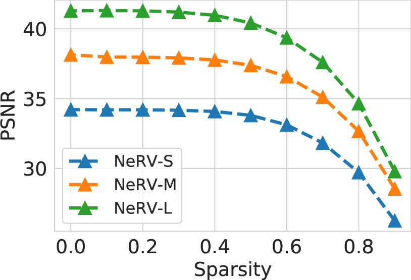
Figure 4: Model pruning. Sparsity is the ratio of parameters pruned.

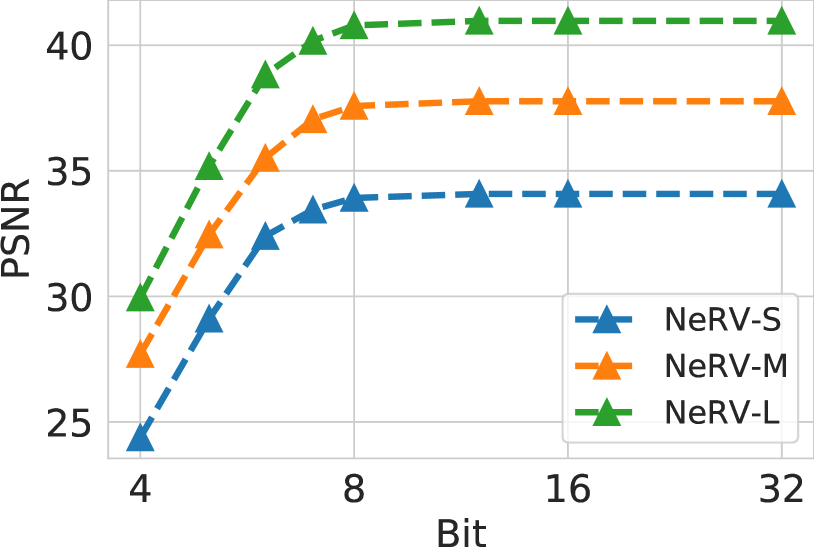
Figure 5: Model quantization. Bit is the bit length used to represent parameter value.

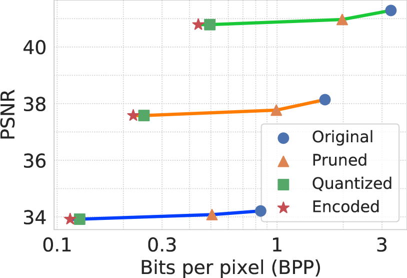
Figure 6: Compression pipeline to show how much each step contribute to compression ratio.

Compare with state-of-the-arts methods. We then compare with state-of-the-arts methods on UVG dataset. First, we concatenate 7 videos into one single video along the time dimension and train NeRV on all the frames from different videos, which we found to be more beneficial than training a single model for each video. After training the network, we apply model pruning, quantization, and weight encoding as described in Section3.2. Figure 8 and Figure 8 show the rate-distortion curves. We compare with H.264 [8], HEVC [2], STAT-SSF-SP [56], HLVC [26], Scale-space [25], and Wu et al. [24]. H.264 and HEVC are performed with medium preset mode. As the first image-wise neural representation, NeRV generally achieves comparable performance with traditional video compression techniques and other learning-based video compression approaches. It is worth noting that when BPP is small, NeRV can match the performance of the state-of-the-art method, showing its great potential in high-rate video compression. When BPP becomes large, the performance gap is mostly because of the lack of full training due to GPU resources limitations. As shown in Table 3, the decoding video quality keeps increasing when the training epochs are longer. Figure 9 shows visualizations for decoding frames. At similar memory budget, NeRV shows image details with better quality.

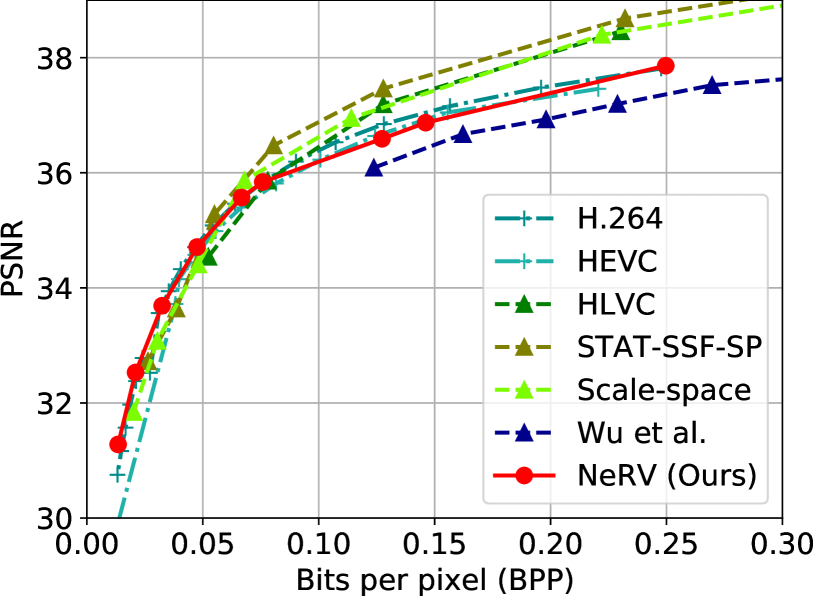
Figure 7: PSNR vs. BPP on UVG dataset.

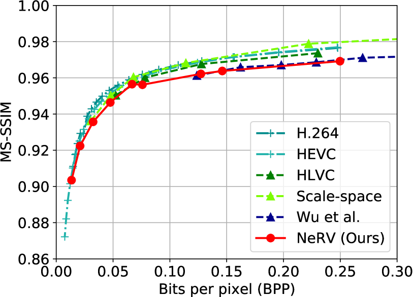
Figure 8: MS-SSIM vs. BPP on UVG dataset.

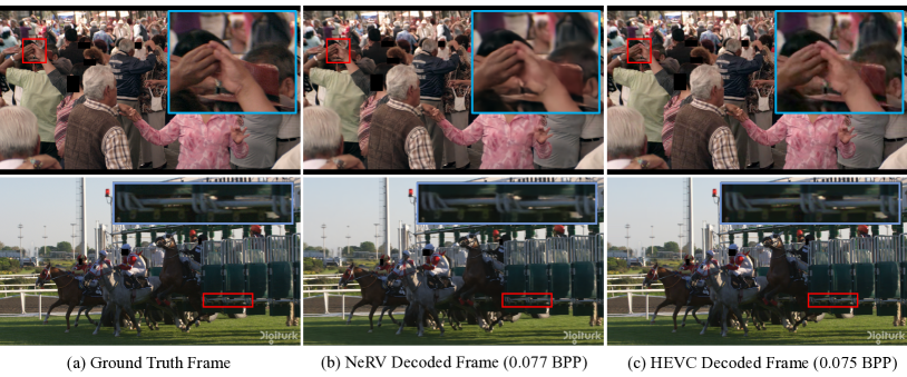
Figure 9: Video compression visualization. At similar BPP, NeRV reconstructs videos with better details.

Decoding time We compare with other methods for decoding time under a similar memory budget. Note that HEVC is run on CPU, while all other learning-based methods are run on a single GPU, including our NeRV. We speedup NeRV by running it in half precision (FP16). Due to the simple decoding process (feedforward operation), NeRV shows great advantage, even for carefully-optimized H.264. And lots of speepup can be expected by running quantizaed model on special hardware. All the other video compression methods have two types of frames: key and interval frames. Key frame can be reconstructed by its encoded feature only while the interval frame reconstruction is also based on the reconstructed key frames. Since most video frames are interval frames, their decoding needs to be done in a sequential manner after the reconstruction of the respective key frames. On the contrary, our NeRV can output frames at any random time index independently, thus making parallel decoding much simpler. This can be viewed as a distinct advantage over other methods.

4.4 Video Denoising

We apply several common noise patterns on the original video and train the model on the perturbed ones. During training, no masks or noise locations are provided to the model, i.e., the target of the model is the noisy frames while the model has no extra signal of whether the input is noisy or not. Surprisingly, our model tries to avoid the influence of the noise and regularizes them implicitly with little harm to the compression task simultaneously, which can serve well for most partially distorted videos in practice.

The results are compared with some standard denoising methods including Gaussian, uniform, and median filtering. These can be viewed as denoising upper bound for any additional compression process. As listed in Table 5, the PSNR of NeRV output is usually much higher than the noisy frames although it’s trained on the noisy target in a fully supervised manner, and has reached an acceptable level for general denoising purpose. Specifically, median filtering has the best performance among the traditional denoising techniques, while NeRV outperforms it in most cases or is at least comparable without any extra denoising design in both architecture design and training strategy.

Table 4: Decoding speed with BPP 0.2 for 1080p videos

Methods	FPS $\uparrow$
Habibian et al. [14]	$10^{-3.7}$
Wu et al. [24]	$10^{-3}$
Rippel et al. [57]	1
DVC [3]	1.8
Liu et al [58]	3
H.264 [8]	9.2
NeRV (FP32)	5.6
NeRV (FP16)	12.5

Table 5: PSNR results for video denoising. “baseline” refers to the noisy frames before any denoising

noise	white $\uparrow$	black $\uparrow$	salt & pepper $\uparrow$	random $\uparrow$	Average $\uparrow$
Baseline	27.85	28.29	27.95	30.95	28.74
Gaussian	30.27	30.14	30.23	30.99	30.41
Uniform	29.11	29.06	29.10	29.63	29.22
Median	33.89	33.84	33.87	33.89	33.87
Minimum	20.55	16.60	18.09	18.20	18.36
Maximum	16.16	20.26	17.69	17.83	17.99
NeRV	33.31	34.20	34.17	34.80	34.12

We also compare NeRV with another neural-network-based denoising method, Deep Image Prior (DIP) [59]. Although its main target is image denoising, NeRV outperforms it in both qualitative and quantitative metrics, demonstrated in Figure 10. The main difference between them is that denoising of DIP only comes form architecture prior, while the denoising ability of NeRV comes from both architecture prior and data prior. DIP emphasizes that its image prior is only captured by the network structure of Convolution operations because it only feeds on a single image. But the training data of NeRV contain many video frames, sharing lots of visual contents and consistences. As a result, image prior is captured by both the network structure and the training data statistics for NeRV. DIP relies significantly on a good early stopping strategy to prevent it from overfitting to the noise. Without the noise prior, it has to be used with fixed iterations settings, which is not easy to generalize to any random kind of noises as mentioned above. By contrast, NeRV is able to handle this naturally by keeping training because the full set of consecutive video frames provides a strong regularization on image content over noise.

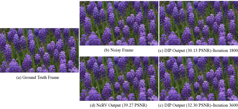
Figure 10: Denoising visualization. (c) and (e) are denoising output for DIP [59]. Data generalization of NeRV leads to robust and better denoising performance since all frames share the same representation, while DIP model overfits one model to one image only.

4.5 Ablation Studies

Finally, we provide ablation studies on the UVG dataset. PSNR and MS-SSIM are adopted for evaluation of the reconstructed videos.
Input embedding. In Table 6, PE means positional encoding as in Equation 1, which greatly improves the baseline, None means taking the frame index as input directly. Similar findings can be found in [4], without any input embedding, the model can not learn high-frequency information, resulting in much lower performance.
Upscale layer. In Table 4.5, we show results of three different upscale methods. i.e., Bilinear Pooling, Transpose Convolution, and PixelShuffle [46]. With similar model sizes, PixelShuffle shows best results. Please note that although Transpose convolution [60] reach comparable results, it greatly slowdown the training speed compared to the PixelShuffle.
Normalization layer. In Table 4.5, we apply common normalization layers in NeRV block. The default setup, without normalization layer, reaches the best performance and runs slightly faster. We hypothesize that the normalization layer reduces the over-fitting capability of the neural network, which is contradictory to our training objective.
Activation layer. Table 4.5 shows results for common activation layers. The GELU [61] activation function achieve the highest performances, which is adopted as our default design.
Loss objective. We show loss objective ablation in Table 10. We shows performance results of different combinations of L2, L1, and SSIM loss. Although adopting SSIM alone can produce the highest MS-SSIM score, but the combination of L1 loss and SSIM loss can achieve the best trade-off between the PSNR performance and MS-SSIM score.

Table 6: Input embedding ablation. PE means positional encoding

	PSNR	MS-SSIM
None	24.93	0.769
PE	37.26	0.970

Table 7: Upscale layer ablation

	PSNR	MS-SSIM
Bilinear Pooling	29.56	0.873
Transpose Conv	36.63	0.967
PixelShuffle	37.26	0.970

Table 8: Norm layer ablation

	PSNR	MS-SSIM
BatchNorm	36.71	0.971
InstanceNorm	35.5	0.963
None	37.26	0.970

Table 9: Activation function ablation

	PSNR	MS-SSIM
ReLU	35.89	0.963
Leaky ReLU	36.76	0.968
Swish	37.08	0.969
GELU	37.26	0.970

Table 10: Loss objective ablation

L2	L1	SSIM	PSNR	MS-SSIM
✓			35.64	0.956
	✓		35.77	0.959
		✓	35.69	0.971
✓	✓		35.95	0.960
✓		✓	36.46	0.970
	✓	✓	37.26	0.970

5 Discussion

Conclusion. In this work, we present a novel neural representation for videos, NeRV, which encodes videos into neural networks. Our key sight is that by directly training a neural network with video frame index and output corresponding RGB image, we can use the weights of the model to represent the videos, which is totally different from conventional representations that treat videos as consecutive frame sequences. With such a representation, we show that by simply applying general model compression techniques, NeRV can match the performances of traditional video compression approaches for the video compression task, without the need to design a long and complex pipeline. We also show that NeRV can outperform standard denoising methods. We hope that this paper can inspire further research works to design novel class of methods for video representations.

Limitations and Future Work. There are some limitations with the proposed NeRV. First, to achieve the comparable PSNR and MS-SSIM performances, the training time of our proposed approach is longer than the encoding time of traditional video compression methods. Second, the architecture design of NeRV is still not optimal yet, we believe more exploration on the neural architecture design can achieve higher performances. Finally, more advanced and cutting the edge model compression methods can be applied to NeRV and obtain higher compression ratios.

Acknowledgement. This project was partially funded by the DARPA SAIL-ON (W911NF2020009) program, an independent grant from Facebook AI, and Amazon Research Award to AS.

Appendix A Appendix

A.1 NeRV Architecture

We provide the architecture details in Table 11. On a $1920\times 1080$ video, given the timestamp index $t$, we first apply a 2-layer MLP on the output of positional encoding layer, then we stack 5 NeRV blocks with upscale factors 5, 3, 2, 2, 2 respectively. In UVG experiments on video compression task, we train models with different sizes by changing the value of $C_{1},C_{2}$ to (48,384), (64,512), (128,512), (128,768), (128,1024), (192,1536), and (256,2048).

Table 11: NeRV architecture for $1920\times 1080$ videos. Change the value of $C_{1}$ and $C_{2}$ to get models with different sizes.

Layer	Modules	Upscale Factor	Output Size & $(C\times H\times W)$
0	Positional Encoding	-	$160\times 1\times 1$
1	MLP & Reshape	-	$C_{1}\times 16\times 9$
2	NeRV block	$5\times$	$C_{2}\times 80\times 45$
3	NeRV block	$3\times$	$C_{2}/2\times 240\times 135$
4	NeRV block	$2\times$	$C_{2}/4\times 480\times 270$
5	NeRV block	$2\times$	$C_{2}/8\times 960\times 540$
6	NeRV block	$2\times$	$C_{2}/16\times 1920\times 1080$
7	Head layer	-	$3\times 1920\times 1080$

A.2 Results on MCL-JCL dataset

We provide the experiment results for video compression task on MCL-JCL [55]dataset in Figure 11(a) and Figure 11(b).

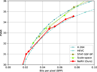
(a)

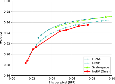
(b)

Figure 11: Rate distortion plots on the MCL-JCV dataset.

A.3 Implementation Details of Baselines

Following prior works, we used ffmpeg [62] to produce the evaluation metrics for H.264 and HEVC.

First, we use the following command to extract frames from original YUV videos, as well as compressed videos to calculate metrics:

⬇

ffmpeg -i FILE.y4m FILE/f%05d.png

Then we use the following commands to compress videos with H.264 or HEVC codec under medium settings:

⬇

ffmpeg -i FILE/f%05d.png -c:v h264 -preset medium \

-bf 0 -crf CRF FILE.EXT

⬇

ffmpeg -i FILE/f%05d.png -c:v hevc -preset medium \

-x265-params bframes=0 -crf CRF FILE.EXT

where FILE is the filename, CRF is the Constant Rate Factor value, and EXT is the video container format extension.

A.4 Video Temporal Interpolation

We also explore NeRV for video temporal interpolation task. Specifically, we train our model with a subset of frames sampled from one video, and then use the trained model to infer/predict unseen frames given an unseen interpolated frame index. As we show in Fig 12, NeRV can give quite reasonable predictions on the unseen frame, which has good and comparable visual quality compared to the adjacent seen frames.

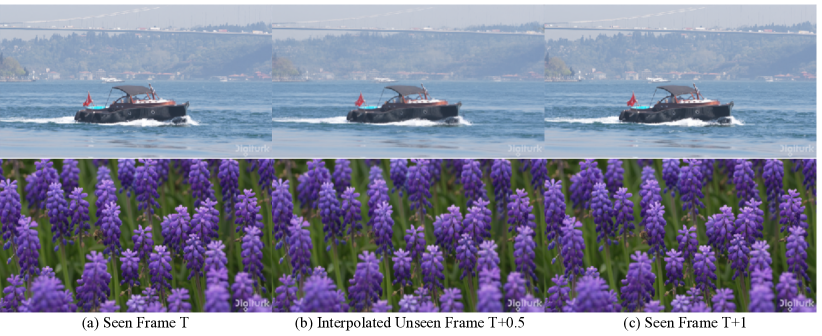
Figure 12: Temporal interpolation results for video with small motion.

A.5 More Visualizations

We provide more qualitative visualization results in Figure 13 to compare the our NeRV with H.265 for the video compression task. We test a smaller model on “Bosphorus” video, and it also has a better performance compared to H.265 codec with similar BPP. The zoomed areas show that our model produces fewer artifacts and the output is smoother.

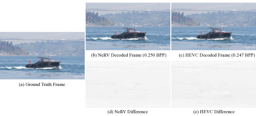
Figure 13: Video compression visulization. The difference is calculated by the L1 loss (absolute value, scaled by the same level for the same frame, and the darker the more different). “Bosphorus” video in UVG dataset, the residual visulization is much smaller for NeRV.

Broader Impact.

As the most popular media format nowadays, videos are generally viewed as frames of sequences. Different from that, our proposed NeRV is a novel way to represent videos as a function of time, parameterized by the neural network, which is more efficient and might be used in many video-related tasks, such as video compression, video denoising and so on. Hopefully, this can potentially save bandwidth, fasten media streaming, which enrich entertainment potentials. Unfortunately, like many advances in deep learning for videos, this approach can be utilized for a variety of purposes beyond our control.

References

- [1] Kurt Hornik, Maxwell Stinchcombe, and Halbert White. Multilayer feedforward networks are universal approximators. Neural networks, 2(5):359–366, 1989.
- [2] Gary J Sullivan, Jens-Rainer Ohm, Woo-Jin Han, and Thomas Wiegand. Overview of the high efficiency video coding (hevc) standard. IEEE Transactions on circuits and systems for video technology, 22(12):1649–1668, 2012.
- [3] Guo Lu, Wanli Ouyang, Dong Xu, Xiaoyun Zhang, Chunlei Cai, and Zhiyong Gao. Dvc: An end-to-end deep video compression framework. In CVPR, 2019.
- [4] Ben Mildenhall, Pratul P Srinivasan, Matthew Tancik, Jonathan T Barron, Ravi Ramamoorthi, and Ren Ng. Nerf: Representing scenes as neural radiance fields for view synthesis. In European Conference on Computer Vision, pages 405–421. Springer, 2020.
- [5] Vincent Sitzmann, Julien Martel, Alexander Bergman, David Lindell, and Gordon Wetzstein. Implicit neural representations with periodic activation functions. Advances in Neural Information Processing Systems, 33, 2020.
- [6] Matthew Tancik, Pratul P Srinivasan, Ben Mildenhall, Sara Fridovich-Keil, Nithin Raghavan, Utkarsh Singhal, Ravi Ramamoorthi, Jonathan T Barron, and Ren Ng. Fourier features let networks learn high frequency functions in low dimensional domains. NeurIPS, 2020.
- [7] Alexandre Mercat, Marko Viitanen, and Jarno Vanne. Uvg dataset: 50/120fps 4k sequences for video codec analysis and development. In Proceedings of the 11th ACM Multimedia Systems Conference, pages 297–302, 2020.
- [8] Thomas Wiegand, Gary J Sullivan, Gisle Bjontegaard, and Ajay Luthra. Overview of the h. 264/avc video coding standard. IEEE Transactions on circuits and systems for video technology, 13(7):560–576, 2003.
- [9] Kyle Genova, Forrester Cole, Daniel Vlasic, Aaron Sarna, William T Freeman, and Thomas Funkhouser. Learning shape templates with structured implicit functions. In Proceedings of the IEEE/CVF International Conference on Computer Vision, pages 7154–7164, 2019.
- [10] Kyle Genova, Forrester Cole, Avneesh Sud, Aaron Sarna, and Thomas A Funkhouser. Deep structured implicit functions. 2019.
- [11] Vincent Sitzmann, Michael Zollhöfer, and Gordon Wetzstein. Scene representation networks: Continuous 3d-structure-aware neural scene representations. arXiv preprint arXiv:1906.01618, 2019.
- [12] Chiyu Jiang, Avneesh Sud, Ameesh Makadia, Jingwei Huang, Matthias Nießner, Thomas Funkhouser, et al. Local implicit grid representations for 3d scenes. In Proceedings of the IEEE/CVF Conference on Computer Vision and Pattern Recognition, pages 6001–6010, 2020.
- [13] Songyou Peng, Michael Niemeyer, Lars Mescheder, Marc Pollefeys, and Andreas Geiger. Convolutional occupancy networks. arXiv preprint arXiv:2003.04618, 2, 2020.
- [14] Rohan Chabra, Jan E Lenssen, Eddy Ilg, Tanner Schmidt, Julian Straub, Steven Lovegrove, and Richard Newcombe. Deep local shapes: Learning local sdf priors for detailed 3d reconstruction. In European Conference on Computer Vision, pages 608–625. Springer, 2020.
- [15] Michael Niemeyer, Lars Mescheder, Michael Oechsle, and Andreas Geiger. Differentiable volumetric rendering: Learning implicit 3d representations without 3d supervision. In Proceedings of the IEEE/CVF Conference on Computer Vision and Pattern Recognition, pages 3504–3515, 2020.
- [16] Michael Oechsle, Lars Mescheder, Michael Niemeyer, Thilo Strauss, and Andreas Geiger. Texture fields: Learning texture representations in function space. In Proceedings of the IEEE/CVF International Conference on Computer Vision, pages 4531–4540, 2019.
- [17] Emilien Dupont, Adam Goliński, Milad Alizadeh, Yee Whye Teh, and Arnaud Doucet. Coin: Compression with implicit neural representations. arXiv preprint arXiv:2103.03123, 2021.
- [18] Gregory K Wallace. The jpeg still picture compression standard. IEEE transactions on consumer electronics, 38(1):xviii–xxxiv, 1992.
- [19] Athanassios Skodras, Charilaos Christopoulos, and Touradj Ebrahimi. The jpeg 2000 still image compression standard. IEEE Signal processing magazine, 18(5):36–58, 2001.
- [20] Didier Le Gall. Mpeg: A video compression standard for multimedia applications. Communications of the ACM, 34(4):46–58, 1991.
- [21] Nasir Ahmed, T_ Natarajan, and Kamisetty R Rao. Discrete cosine transform. IEEE transactions on Computers, 100(1):90–93, 1974.
- [22] Marc Antonini, Michel Barlaud, Pierre Mathieu, and Ingrid Daubechies. Image coding using wavelet transform. IEEE Transactions on image processing, 1(2):205–220, 1992.
- [23] Zhengxue Cheng, Heming Sun, Masaru Takeuchi, and Jiro Katto. Learning image and video compression through spatial-temporal energy compaction. In Proceedings of the IEEE/CVF Conference on Computer Vision and Pattern Recognition, pages 10071–10080, 2019.
- [24] Chao-Yuan Wu, Nayan Singhal, and Philipp Krahenbuhl. Video compression through image interpolation. In Proceedings of the European Conference on Computer Vision (ECCV), pages 416–431, 2018.
- [25] Eirikur Agustsson, David Minnen, Nick Johnston, Johannes Balle, Sung Jin Hwang, and George Toderici. Scale-space flow for end-to-end optimized video compression. In Proceedings of the IEEE/CVF Conference on Computer Vision and Pattern Recognition, pages 8503–8512, 2020.
- [26] Ren Yang, Fabian Mentzer, Luc Van Gool, and Radu Timofte. Learning for video compression with hierarchical quality and recurrent enhancement. In Proceedings of the IEEE/CVF Conference on Computer Vision and Pattern Recognition, pages 6628–6637, 2020.
- [27] Vincent Vanhoucke, Andrew Senior, and Mark Z Mao. Improving the speed of neural networks on cpus. 2011.
- [28] Suyog Gupta, Ankur Agrawal, Kailash Gopalakrishnan, and Pritish Narayanan. Deep learning with limited numerical precision. In International conference on machine learning, pages 1737–1746. PMLR, 2015.
- [29] Song Han, Huizi Mao, and William J Dally. Deep compression: Compressing deep neural networks with pruning, trained quantization and huffman coding. arXiv preprint arXiv:1510.00149, 2015.
- [30] Wei Wen, Chunpeng Wu, Yandan Wang, Yiran Chen, and Hai Li. Learning structured sparsity in deep neural networks. arXiv preprint arXiv:1608.03665, 2016.
- [31] Benoit Jacob, Skirmantas Kligys, Bo Chen, Menglong Zhu, Matthew Tang, Andrew Howard, Hartwig Adam, and Dmitry Kalenichenko. Quantization and training of neural networks for efficient integer-arithmetic-only inference. In Proceedings of the IEEE Conference on Computer Vision and Pattern Recognition, pages 2704–2713, 2018.
- [32] Raghuraman Krishnamoorthi. Quantizing deep convolutional networks for efficient inference: A whitepaper. arXiv preprint arXiv:1806.08342, 2018.
- [33] Roberto Rigamonti, Amos Sironi, Vincent Lepetit, and Pascal Fua. Learning separable filters. In Proceedings of the IEEE conference on computer vision and pattern recognition, pages 2754–2761, 2013.
- [34] Emily Denton, Wojciech Zaremba, Joan Bruna, Yann LeCun, and Rob Fergus. Exploiting linear structure within convolutional networks for efficient evaluation. arXiv preprint arXiv:1404.0736, 2014.
- [35] Max Jaderberg, Andrea Vedaldi, and Andrew Zisserman. Speeding up convolutional neural networks with low rank expansions. arXiv preprint arXiv:1405.3866, 2014.
- [36] Taco Cohen and Max Welling. Group equivariant convolutional networks. In International conference on machine learning, pages 2990–2999. PMLR, 2016.
- [37] Shuangfei Zhai, Yu Cheng, Weining Lu, and Zhongfei Zhang. Doubly convolutional neural networks. arXiv preprint arXiv:1610.09716, 2016.
- [38] Wenling Shang, Kihyuk Sohn, Diogo Almeida, and Honglak Lee. Understanding and improving convolutional neural networks via concatenated rectified linear units. In international conference on machine learning, pages 2217–2225. PMLR, 2016.
- [39] Sander Dieleman, Jeffrey De Fauw, and Koray Kavukcuoglu. Exploiting cyclic symmetry in convolutional neural networks. In International conference on machine learning, pages 1889–1898. PMLR, 2016.
- [40] Lei Jimmy Ba and Rich Caruana. Do deep nets really need to be deep? arXiv preprint arXiv:1312.6184, 2013.
- [41] Geoffrey Hinton, Oriol Vinyals, and Jeff Dean. Distilling the knowledge in a neural network. arXiv preprint arXiv:1503.02531, 2015.
- [42] Guobin Chen, Wongun Choi, Xiang Yu, Tony Han, and Manmohan Chandraker. Learning efficient object detection models with knowledge distillation. In Proceedings of the 31st International Conference on Neural Information Processing Systems, pages 742–751, 2017.
- [43] Antonio Polino, Razvan Pascanu, and Dan Alistarh. Model compression via distillation and quantization. arXiv preprint arXiv:1802.05668, 2018.
- [44] Nasim Rahaman, Aristide Baratin, Devansh Arpit, Felix Draxler, Min Lin, Fred Hamprecht, Yoshua Bengio, and Aaron Courville. On the spectral bias of neural networks. In International Conference on Machine Learning, pages 5301–5310. PMLR, 2019.
- [45] Ashish Vaswani, Noam Shazeer, Niki Parmar, Jakob Uszkoreit, Llion Jones, Aidan N Gomez, Lukasz Kaiser, and Illia Polosukhin. Attention is all you need. arXiv preprint arXiv:1706.03762, 2017.
- [46] Wenzhe Shi, Jose Caballero, Ferenc Huszár, Johannes Totz, Andrew P Aitken, Rob Bishop, Daniel Rueckert, and Zehan Wang. Real-time single image and video super-resolution using an efficient sub-pixel convolutional neural network. In Proceedings of the IEEE conference on computer vision and pattern recognition, pages 1874–1883, 2016.
- [47] Ron Banner, Itay Hubara, Elad Hoffer, and Daniel Soudry. Scalable methods for 8-bit training of neural networks. arXiv preprint arXiv:1805.11046, 2018.
- [48] Fartash Faghri, Iman Tabrizian, Ilia Markov, Dan Alistarh, Daniel Roy, and Ali Ramezani-Kebrya. Adaptive gradient quantization for data-parallel sgd. arXiv preprint arXiv:2010.12460, 2020.
- [49] Naigang Wang, Jungwook Choi, Daniel Brand, Chia-Yu Chen, and Kailash Gopalakrishnan. Training deep neural networks with 8-bit floating point numbers. arXiv preprint arXiv:1812.08011, 2018.
- [50] David A Huffman. A method for the construction of minimum-redundancy codes. Proceedings of the IRE, 40(9):1098–1101, 1952.
- [51] Diederik P Kingma and Jimmy Ba. Adam: A method for stochastic optimization. arXiv preprint arXiv:1412.6980, 2014.
- [52] Ilya Loshchilov and Frank Hutter. Sgdr: Stochastic gradient descent with warm restarts. arXiv preprint arXiv:1608.03983, 2016.
- [53] Zhou Wang, Eero P Simoncelli, and Alan C Bovik. Multiscale structural similarity for image quality assessment. In The Thrity-Seventh Asilomar Conference on Signals, Systems Computers, 2003, volume 2, pages 1398–1402. Ieee, 2003.
- [54] Adam Paszke, Sam Gross, Francisco Massa, Adam Lerer, James Bradbury, Gregory Chanan, Trevor Killeen, Zeming Lin, Natalia Gimelshein, Luca Antiga, Alban Desmaison, Andreas Kopf, Edward Yang, Zachary DeVito, Martin Raison, Alykhan Tejani, Sasank Chilamkurthy, Benoit Steiner, Lu Fang, Junjie Bai, and Soumith Chintala. Pytorch: An imperative style, high-performance deep learning library. In H. Wallach, H. Larochelle, A. Beygelzimer, F. d'Alché-Buc, E. Fox, and R. Garnett, editors, Advances in Neural Information Processing Systems 32, pages 8024–8035. Curran Associates, Inc., 2019.
- [55] Haiqiang Wang, Weihao Gan, Sudeng Hu, Joe Yuchieh Lin, Lina Jin, Longguang Song, Ping Wang, Ioannis Katsavounidis, Anne Aaron, and C-C Jay Kuo. Mcl-jcv: a jnd-based h. 264/avc video quality assessment dataset. In 2016 IEEE International Conference on Image Processing (ICIP), pages 1509–1513. IEEE, 2016.
- [56] Ruihan Yang, Yibo Yang, Joseph Marino, and Stephan Mandt. Hierarchical autoregressive modeling for neural video compression. arXiv preprint arXiv:2010.10258, 2020.
- [57] Oren Rippel, Sanjay Nair, Carissa Lew, Steve Branson, Alexander G Anderson, and Lubomir Bourdev. Learned video compression. In ICCV, 2019.
- [58] Jerry Liu, Shenlong Wang, Wei-Chiu Ma, Meet Shah, Rui Hu, Pranaab Dhawan, and Raquel Urtasun. Conditional entropy coding for efficient video compression. In ECCV, 2020.
- [59] Dmitry Ulyanov, Andrea Vedaldi, and Victor Lempitsky. Deep image prior. In Proceedings of the IEEE conference on computer vision and pattern recognition, pages 9446–9454, 2018.
- [60] Vincent Dumoulin and Francesco Visin. A guide to convolution arithmetic for deep learning. arXiv preprint arXiv:1603.07285, 2016.
- [61] Dan Hendrycks and Kevin Gimpel. Gaussian error linear units (gelus). arXiv preprint arXiv:1606.08415, 2016.
- [62] Suramya Tomar. Converting video formats with ffmpeg. Linux Journal, 2006(146):10, 2006.