Dynamic Causal Bayesian Optimization

Abstract

This paper studies the problem of performing a sequence of optimal interventions in a causal dynamical system where both the target variable of interest and the inputs evolve over time. This problem arises in a variety of domains e.g. system biology and operational research. Dynamic Causal Bayesian Optimization (dcbo) brings together ideas from sequential decision making, causal inference and Gaussian process (gp) emulation. dcbo is useful in scenarios where all causal effects in a graph are changing over time. At every time step dcbo identifies a local optimal intervention by integrating both observational and past interventional data collected from the system. We give theoretical results detailing how one can transfer interventional information across time steps and define a dynamic causal gp model which can be used to quantify uncertainty and find optimal interventions in practice. We demonstrate how dcbo identifies optimal interventions faster than competing approaches in multiple settings and applications.

1 Introduction

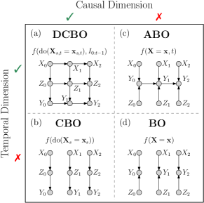
Figure 1: dag representation of a dynamic causal global optimisation (dcgo) problem (a) and the dag considered when using cbo, abo or bo to address the same problem. Shaded nodes gives observed variables while the arrows represent causal effects.

Solving decision making problems in a variety of domains requires understanding of cause-effect relationships in a system. This can be obtained by experimentation. However, deciding how to intervene at every point in time is particularly complex in dynamical systems, due to the evolving nature of causal effects. For instance, companies need to decide how to allocate scarce resources across different quarters. In system biology, scientists need to identify genes to knockout at specific points in time. This paper describes a probabilistic framework that finds such optimal interventions over time.

Focusing on a specific example, consider a setting in which $Y_{t}$ denotes the unemployment-rate of an economy at time $t$, $Z_{t}$ is the economic growth and $X_{t}$ the inflation rate. Fig. 1a depicts the causal graph [44] representing an agent’s understanding of the causal links between these variables. The agent aims to determine, at each time step $t\in\{0,1,2\}$, the optimal action to perform in order to minimize the current unemployment rate $Y_{t}$ while accounting for the intervention cost. The investigator could frame this setting as a sequence of global optimization problems and find the solutions by resorting to Causal Bayesian Optimization [cbo, 4]. cbo extends Bayesian Optimization [bo, 50] to cases in which the variable to optimize is part of a causal model where a sequence of interventions can be performed. However, cbo does not account for the system’s temporal evolution thus breaking the time dependency structure existing among variables (Fig. 1b). This will lead to sub-optimal solutions, especially in non-stationary scenarios. The same would happen when using Adaptive Bayesian Optimization [abo, 43] (Fig. 1c) or bo (Fig. 1d). abo captures the time dependency of the objective function but neither considers the causal structure among inputs nor their temporal evolution. bo disregards both the temporal and the causal structure. Our setting differs from both reinforcement learning (rl) and the multi-armed bandits setting (mab). Differently from mab we consider interventions on continuous variables where the dynamic target variable has a non-stationary interventional distribution. In addition, compared to rl, we do not model the state dynamics explicitly and allow the agent to perform a number of explorative interventions which do not change the underlying state of the system, before selecting the optimal action. We discuss these points further in Section 1.1.

Dynamic Causal Bayesian Optimization, henceforth dcbo, accounts for both the causal relationships among input variables and the causality between inputs and outputs which might evolve over time. dcbo integrates cbo with dynamic Bayesian networks (dbn), offering a novel approach for decision making under uncertainty within dynamical systems. dbn [32] are commonly used in time-series modelling and carry dependence assumptions that do not imply causation. Instead, in probabilistic causal models [45], which form the basis for the cbo framework, graphs are buildt around causal information and allow us to reason about the effects of different interventions. By combining cbo with dbns, the proposed methodology finds an optimal sequence of interventions which accounts for the causal temporal dynamics of the system. In addition, dcbo takes into account past optimal interventions and transfers this information across time, thus identifying the optimal intervention faster than competing approaches and at a lower cost. We make the following contributions:

• We formulate a new class of optimization problems called Dynamic Causal Global Optimization (dcgo) where the objective functions account for the temporal causal dynamics among variables.

• We give theoretical results demonstrating how interventional information can be transferred across time-steps depending on the topology of the causal graph.

• Exploiting our theoretical results, we solve the optimization problem with dcbo. At every time step, dcbo constructs surrogate models for different intervention sets by integrating various sources of data while accounting for past interventions.

• We analyze dcbo performance in a variety of settings comparing against cbo, abo and bo.

1.1 Related Work

Dynamic Optimization Optimization in dynamic environments has been studied in the context of evolutionary algorithms [21, 26]. More recently, other optimization techniques [46, 53, 16] have been adapted to dynamic settings, see e.g. [14] for a review. Focusing on bo, the literature on dynamic settings [5, 9, 43] is limited. The dynamic bo framework closest to this work is given by Nyikosa et al. [43] and focuses on functions defined on continuous spaces that follow a more complex behaviour than a simple Markov model. abo treats the inputs as fixed and not as random variables, thereby disregarding their temporal evolution and, more importantly, breaking their causal dependencies.

Causal Optimization Causal bo [cbo, 4] focuses instead on the causal aspect of optimization and solves the problem of finding an optimal intervention in a dag by modelling the intervention functions with single gps or a multi-task gp model [3]. cbo disregards the existence of a temporal evolution in both the inputs and the output variable, treating them as i.i.d. overtime. While disregarding time significantly simplifies the problem, it prevents the identification of an optimal intervention at every $t$.

Bandits and rl In the broader decision-making literature, causal relationships have been considered in the context of bandits [6, 35, 36, 37] and reinforcement learning [38, 11, 20, 58, 39]. In these cases, actions or arms, correspond to interventions on a causal graph where there exists complex relationships between the agent’s decisions and the received rewards. While dynamic settings have been considered in acausal bandit algorithms [7, 54, 57], causal mab have focused on static settings. Dynamic settings are instead considered by rl algorithms and formalized through Markov decision processes (mdp). In the current formulation, dcbo does not consider an mdp as we do not have a notion of state and therefore do not require an explicit model of its dynamics. The system is fully specified by the causal model. As in bo, we focus on identifying a set of time-indexed optimal actions rather than an optimal policy. We allow the agent to perform explorative interventions that do not lead to state transitions. More importantly, differently from both mab and rl, we allow for the integration of both observational and interventional data. An expanded discussion on the reason why dcbo should be used and the links between dcbo, cbo, abo and rl is included in the supplement (Appendix H).

2 Background and Problem Statement

Let random variables and values be denoted by upper-case and lower-case letters respectively. Vectors are represented shown in bold. $\operatorname{do}\!\left(X=x\right)$ represents an intervention on $X$ whose value is set to $x$. $p(Y\mid X=x)$ represents an observational distribution and $p(Y\mid\operatorname{do}\!\left(X=x\right))$ represents an interventional distribution. This is the distribution of $Y$ obtained by intervening on $X$ and fixing its value to $x$ in the data generating mechanism (see Fig. 2), irrespective of the values of its parents. Evaluating $p(Y\mid\operatorname{do}\!\left(X=x\right))$ requires “real” interventions while $p(Y\mid X=x)$ only requires “observing” the system. $\mathcal{D}^{O}$ and $\mathcal{D}^{I}$ denote observational and interventional datasets respectively. Consider a structural causal model (scm) defined in Definition 1.

Definition 1.

(Structural Causal Model) [45, p. 203]. A structural causal model $M$ is a triple $\left\langle\mathbf{U},\mathbf{V},F)\right\rangle$ where $\mathbf{U}$ is a set of background variables (also called exogenous), that are determined by factors outside of the model. $\mathbf{V}$ is a set $\{V_{1},V_{2},\ldots,V_{|\mathbf{V}|}\}$ of observable variables (also called endogenous), that are determined by variables in the model (i.e., determined by variables in $\mathbf{U}\cup\mathbf{V}$). $F$ is a set of functions $\{f_{1},f_{2},\ldots,f_{n}\}$ such that each $f_{i}$ is a mapping from the respective domains of $U_{i}\cup\text{Pa}\!\left(V_{i}\right)$ to $V_{i}$, where $U_{i}\subseteq\mathbf{U}$ and $\text{Pa}\!\left(V_{i}\right)\subseteq\mathbf{V}\setminus V_{i}$ and the entire set $F$ forms a mapping from $\mathbf{U}$ to $\mathbf{V}$. In other words, each $\{f_{i}\in v_{i}\leftarrow f_{i}(\text{Pa}\!\left(v_{i}\right),u_{i})\mid i=1,\ldots,n\}$, assigns a value to $V_{i}$ that depends on the values of the select set of variables $(U_{i}\cup\text{Pa}\!\left(V_{i}\right))$.

$M$ is associated to a directed acyclic graph (dag) $\mathcal{G}$, in which each node corresponds to a variable and the directed edges point from members of $\text{Pa}(V_{i})$ and $U_{i}$ to $V_{i}$. We assume $\mathcal{G}$ to be known and leave the integration with causal discovery [25] methods for future work. Within $\mathbf{V}$, we distinguish between three different types of variables: non-manipulative variables $\mathbf{C}$, which cannot be modified, treatment variables $\mathbf{X}$ that can be set to specific values and output variable $Y$ that represents the agent’s outcome of interest. Exploiting the rules of do-calculus [45] one can compute $p(Y\mid\operatorname{do}\!\left(X=x\right))$ using observational data. This often involves evaluating intractable integrals which can be approximated by using observational data to get a Monte Carlo estimate $\widehat{p}(Y\mid\operatorname{do}\!\left(X=x\right))\approx p(Y\mid\operatorname{do}\!\left(X=x\right))$. These approximations will be consistent when the number of samples drawn from $p(\mathbf{V})$ is large.

Causality in time

One can encode the existence of causal mechanisms across time steps by explicitly representing these relationships with edges in an extended graph denoted by $\mathcal{G}_{0:T}$. For instance, the dag in Fig. 1(a) can be seen as one of the dags in Fig. 1(b) propagated in time. The dag in Fig. 1(a) captures both the causal structure existing across time steps and the causal mechanism within every “time-slice” $t$ [32]. In order to reason about interventions that are implemented in a sequential manner, that is at time $t$ we decide which intervention to perform in the system and so define:

Definition 2.

$M_{t}$ is the scm at time step $t$ defined as $M_{t}=\left\langle\mathbf{U}_{0:t},\mathbf{V}_{0:t},\mathbf{F}_{0:t}\right\rangle$ where $0:t$ denotes the union of the corresponding variables or functions up to time $t$ (see Fig. 2). $\mathbf{V}_{0:t}$ includes $\mathbf{X}_{0:t}=\mathbf{X}_{t}$, $\mathbf{Y}_{0:t}=Y_{t}$ and $\mathbf{C}_{0:t}=\mathbf{C}_{t}\cup\mathbf{C}_{0:t-1}$. The functions in $\mathbf{F}_{0:t}$ corresponding to intervened variables are replaced by constant values while the exogenous variables related to them are excluded from $\mathbf{U}_{0:t}$.

Definition 3.

$\mathcal{G}_{t}$ is the causal graph associated to $M_{t}$. In $\mathcal{G}_{t}$, the incoming edges in variables intervened at $0:t-1$ are mutilated while intervened variables are represented by deterministic nodes (squares) – see Fig. 2.

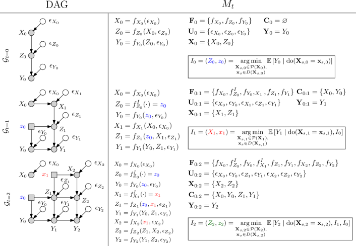
Figure 2: Structural equation models considered by dcbo at every time step $t\in\{0,1,2\}$. Exogenous noise variables $\epsilon_{i}$ are depicted here but are omitted in the remainder of the paper, to avoid clutter. For every $t$, $\mathcal{G}_{t}$ is a mutilated version of $\mathcal{G}_{t-1}$ reflecting the optimal intervention implemented in the system at $0:t-1$ which are represented by squares. The scm functions in $\mathbf{F}_{0:t}$ corresponding to the intervened variables are set to constant values. The exogenous variables that only related to the intervened variables are excluded from $U_{t}$. $\mathbf{C}_{0:t}$ is given by the set $\{\mathbf{C}_{t}\cup\mathbf{C}_{0:t-1}\cup\mathbf{Y}_{0:t-1}\cup\mathbf{X}_{0:t-1}\}$.

Dynamic Causal Global Optimization (dcgo)

The goal of this work is to find a sequence of interventions, optimizing a target variable, at each time step, in a causal dag. Given $\mathcal{G}_{t}$ and $M_{t}$, at every time step $t$, we wish to optimize $Y_{t}$ by intervening on a subset of the manipulative variables $\mathbf{X}_{t}$. The optimal intervention variables $\mathbf{X}^{\star}_{s,t}$ and intervention levels $\mathbf{x}_{s,t}^{\star}$ are given by:

$$\mathbf{X}_{s,t}^{\star},\mathbf{x}_{s,t}^{\star}=\operatorname*{arg\,min}_{\mathbf{X}_{s,t}\in\mathcal{P}(\mathbf{X}_{t}),\mathbf{x}_{s}\in D(\mathbf{X}_{s,t})}\mathbb{E}{\left[Y_{t}\mid\operatorname{do}\!\left(\mathbf{X}_{s,t}=\mathbf{x}_{s,t}\right),\mathds{1}_{t>0}\cdot I_{0:t-1}\right]}$$ (1)

where $I_{0:t-1}=\bigcup_{i=0}^{t-1}\operatorname{do}\!\left(\mathbf{X}_{s,i}^{\star}=\mathbf{x}_{s,i}^{\star}\right)$ denotes previous interventions, $\mathds{1}_{t>0}$ is the indicator function and $\mathcal{P}(\mathbf{X}_{t})$ is the power set of $\mathbf{X}_{t}$. $D(\mathbf{X}_{s,t})$ represents the interventional domain of $\mathbf{X}_{s,t}$. In the sequel we denote the previously intervened variables by $I_{0:t-1}^{V}=\bigcup_{i=0}^{t-1}\mathbf{X}_{s,i}^{\star}$ and implemented intervention levels by $I_{0:t-1}^{L}=\bigcup_{i=0}^{t-1}\mathbf{x}_{s,i}^{\star}$. The cost of each intervention is given by $\texttt{cost}(\mathbf{X}_{s,t},\mathbf{x}_{s,t})$. In order to solve the problem in Eq. 1 we make the following assumptions :

Assumptions 1.

Denote by $\mathcal{G}(t)$ the causal graph including variables at time $t$ in $\mathcal{G}_{0:T}$ and let $Y_{t}^{\textsc{PT}}=\text{Pa}\!\left(Y_{t}\right)\cap Y_{0:t-1}$ be the set of variables in $\mathcal{G}_{0:T}$ that are both parents of $Y_{t}$ and targets at previous time step. Let the set $Y_{t}^{\textsc{PNT}}=\text{Pa}\!\left(Y_{t}\right)\backslash Y_{t}^{\textsc{PT}}$ be the complement and denote by $f_{Y_{t}}(\cdot)$ the functional mapping for $Y_{t}$ in $M_{t}$. We make the following assumptions:

1. Invariance of causal structure: $\mathcal{G}(t)=\mathcal{G}(0),\forall t>0$.

2. Additivity of $f_{Y_{t}}(\cdot)$ that is $Y_{t}=f_{Y_{t}}(\text{Pa}\!\left(Y_{t}\right))+\epsilon$ with $f_{Y_{t}}(\text{Pa}\!\left(Y_{t}\right))=f_{Y}^{Y}(Y_{t}^{\textsc{PT}})+f_{Y}^{\text{NY}}(Y_{t}^{\textsc{PNT}})$ where $f_{Y}^{Y}$ and $f_{Y}^{\text{NY}}$ are two generic unknown functions and $\epsilon\sim\mathcal{N}(0,\sigma^{2})$.

3. Absence of unobserved confounders in $\mathcal{G}_{0:T}$.

Assumption (3) implies the absence of unobserved confounders at every time step. For instance, this is the case in Fig. 1a. Still in this dag, Assumption (2) implies $f_{Y_{t}}(\text{Pa}\!\left(Y_{t}\right))=f_{Y}^{Y}(Y_{t-1})+f_{Y}^{\text{NY}}(Z_{t})+\epsilon_{Y_{t}},\forall t>0$. Finally, Assumption (1) implies the existence of the same variables at every time step and a constant orientation of the edges among them for $t>0$.

Notice that Assumptions 1 imply invariance of the causal structure within each time-slice, i.e. the structure, edges and vertices, concerning the nodes with the same time index. This means that, across time steps, both the graph and the functional relationships can change. Therefore, not only can the causal effects change significantly across time steps, but also the input dimensionality of the causal functions we model, might change. For instance, in the dag of Fig. 3(c), the target function for $Y_{2}$ has dimensionality 3 and a function $f_{Y_{t}}(\cdot)$ that is completely different from the one assumed for $Y_{1}$ that has only two parents. We can thus model a wide variety of settings and causal effects despite this assumption. Furthermore, even though we assume an additive structure for the functional relationship on $Y$, the use of gps allow us to have flexible models with highly non-linear causal effects across different graph structures. In the causality literature, gp models are well established and have shown good performances compared to parametric linear and non-linear models (see e.g. [51, 56, 59]). The sum of gps gives a flexible and computationally tractable model that can be used to capture highly non-linear causal effects while helping with interpretability [19, 18].

3 Methodology

In this section we introduce Dynamic Causal Bayesian Optimization (dcbo), a novel methodology addressing the problem in Eq. 1. We first study the correlation among objective functions for two consecutive time steps and use it to derive a recursion formula that, based on the topology of the graph, expresses the causal effects at time $t$ as a function of previously implemented interventions (see square nodes in Fig. 2). Exploiting these results, we develop a new surrogate model for the objective functions that can be used within a cbo framework to find the optimal sequence of interventions. This model enables the integration of observational data and interventional data, collected at previous time-steps and interventional data collected at time $t$, thereby accelerating the identification of the current optimal intervention.

3.1 Characterization of the time structure in a dag with time dependent variables

The following result provides a theoretical foundation for the dynamic causal gp model introduced later. In particular, it derives a recursion formula allowing us to express the objective function at time $t$ as a function of the objective functions corresponding to the optimal interventions at previous time steps. The proof is given in the appendix (§B).

Definition 4.

Consider a dag $\mathcal{G}_{0:T}$ and the objective function $\mathbb{E}{\left[Y_{t}\mid\operatorname{do}\!\left(\mathbf{X}_{s,t}=\mathbf{x}_{s,t}\right),I_{0:t-1}\right]}$ for a generic time step $t\in\{0,\dots,T\}$. Denote by $Y_{t}^{\textsc{PT}}=(\text{Pa}\!\left(Y_{t}\right)\cap Y_{0:t-1})$ the parents of $Y_{t}$ that are targets at previous time steps and by $Y_{t}^{\textsc{PNT}}=\text{Pa}\!\left(Y_{t}\right)\backslash Y_{t}^{\textsc{PT}}$ the remaining parents. For any $\mathbf{X}_{s,t}\in\mathcal{P}(\mathbf{X}_{t})$ and $I_{0:t-1}^{V}\subseteq\mathbf{X}_{0:t-1}$ we define the following sets:

• $\mathbf{X}_{s,t}^{\textsc{PY}}=\mathbf{X}_{s,t}\cap\text{Pa}\!\left(Y_{t}\right)$ includes the variables in $\mathbf{X}_{s,t}$ that are parents of $Y_{t}$.

• $I_{0:t-1}^{\textsc{PY}}=I_{0:t-1}^{V}\cap\text{Pa}\!\left(Y_{t}\right)$ includes the variables in $I_{0:t-1}^{V}$ that are parents of $Y_{t}$.

• $W\subset\text{Pa}\!\left(Y_{t}\right)$ such that $\text{Pa}\!\left(Y_{t}\right)=(\text{Pa}\!\left(Y_{t}\right)\cap Y_{0:t-1})\cup\mathbf{X}_{s,t}^{\textsc{PY}}\cup I_{0:t-1}^{\textsc{PY}}\cup W$. $W$ includes variables that are parents of $Y_{t}$ but are not targets nor intervened variables.

The values of $I_{0:t-1}$, $\mathbf{X}_{s,t}^{\textsc{PY}}$, $I_{0:t-1}^{\textsc{PY}}$ and $W$ will be denoted by $\mathbf{i}$, $\mathbf{x}^{\textsc{PY}}$, $\mathbf{i}^{\textsc{PY}}$ and $\mathbf{w}$ respectively.

Theorem 1.

Time operator. Consider a dag $\mathcal{G}_{0:T}$ and the related scm satisfying Assumptions 1. It is possible to prove that, $\forall\mathbf{X}_{s,t}\in\mathcal{P}(\mathbf{X}_{t})$, the intervention function $f_{s,t}(\mathbf{x})=\mathbb{E}{\left[Y_{t}\mid\operatorname{do}\!\left(\mathbf{X}_{s,t}=\mathbf{x}\right),\mathds{1}_{t>0}\cdot I_{0:t-1}\right]}$ with $f_{s,t}(\mathbf{x}):D(\mathbf{X}_{s,t})\to\mathbb{R}$ can be written as:

$$f_{s,t}(\mathbf{x})=f_{Y}^{Y}(\mathbf{f}^{\star})+\mathbb{E}_{p(\mathbf{w}\mid\operatorname{do}\!\left(\mathbf{X}_{s,t}=\mathbf{x}\right),\mathbf{i})}{\left[f_{Y}^{\text{NY}}(\mathbf{x}^{\textsc{PY}},\mathbf{i}^{\textsc{PY}},\mathbf{w})\right]}$$ (2)

where $\mathbf{f}^{\star}=\{\mathbb{E}{\left[Y_{i}|\operatorname{do}\!\left(\mathbf{X}_{s,i}^{\star}=\mathbf{x}_{s,i}^{\star}\right),I_{0:i-1}\right]}\}_{Y_{i}\in Y_{t}^{\textsc{PT}}}$ that is the set of previously observed optimal targets that are parents of $Y_{t}$. $f_{Y}^{Y}$ denotes the function mapping $Y_{t}^{\textsc{PT}}$ to $Y_{t}$ and $f_{Y}^{\text{NY}}$ represents the function mapping $Y_{t}^{\textsc{PNT}}$ to $Y_{t}$.

Eq. 2 reduces to $\mathbb{E}_{p(\mathbf{w}|\operatorname{do}\!\left(\mathbf{X}_{s,t}=\mathbf{x}\right),\mathbf{i})}{\left[f_{Y}^{\text{NY}}(\mathbf{x}^{\textsc{PY}},\mathbf{i}^{\textsc{PY}},\mathbf{w})\right]}$ when $Y_{t}$ does not depend on previous targets. This is the setting considered in cbo that can be thus seen as a particular instance of dcbo. Exploiting Assumptions (1), it is possible to further expand the second term in Eq. 2 to get the following expression. A proof is given in the supplement (§B).

Corollary 1.

Given Assumptions 1, we can write:

$$\mathbb{E}_{p(\mathbf{w}|\operatorname{do}\!\left(\mathbf{X}_{s,t}=\mathbf{x}\right),\mathbf{i})}{\left[f_{Y}^{\text{NY}}(\mathbf{x}^{\textsc{PY}},\mathbf{i}^{\textsc{PY}},\mathbf{w})\right]}=\mathbb{E}_{p(\mathbf{U}_{0:t})}{\left[f_{Y}^{\text{NY}}(\mathbf{x}^{\textsc{PY}},\mathbf{i}^{\textsc{PY}},\{C(W)\}_{W\in\mathbf{W}})\right]}$$ (3)

where $p(\mathbf{U}_{0:t})$ is the distribution for the exogenous variables up to time $t$ and $C(W)$ is given by:

$$C(W)=\begin{cases}f_{W}(\mathbf{u}_{W},\mathbf{x}^{\textsc{PW}},\mathbf{i}^{\textsc{PW}})&\text{if}\quad R=\varnothing\\ f_{W}(\mathbf{u}_{W},\mathbf{x}^{\textsc{PW}},\mathbf{i}^{\textsc{PW}},r)&\text{if}\quad R\subseteq\mathbf{X}_{s,t}\cup I_{0:t-1}^{V}\\ f_{W}(\mathbf{u}_{W},\mathbf{x}^{\textsc{PW}},\mathbf{i}^{\textsc{PW}},C(R))&\text{if}\quad R\not\subseteq\mathbf{X}_{s,t}\cup I_{0:t-1}^{V}\end{cases}$$

where $f_{W}$ represents the functional mapping for $W$ in the scm and $\mathbf{u}_{W}$ is the set of exogenous variables with edges into $W$. $\mathbf{x}^{\textsc{PW}}$ and $\mathbf{i}^{\textsc{PW}}$ are the values corresponding to $\mathbf{X}_{s,t}^{\textsc{PW}}$ and $I_{0:t-1}^{\textsc{PW}}$ which in turn represent the subset of variables in $\mathbf{X}_{s,t}$ and $I_{0:t-1}^{V}$ that are parents of $W$. Finally $r$ is the value of $R=\text{Pa}\!\left(W\right)\backslash(\mathbf{X}_{s,t}^{\textsc{PY}}\cup I_{0:t-1}^{\textsc{PW}})$.

Examples for Eq. 2:

For the dag in Fig. 1(a), at time $t=1$ and with $I_{0:t-1}^{V}=\{Z_{0}\}$, we have $\mathbb{E}{\left[Y\mid\operatorname{do}\!\left(Z_{1}=z\right),I_{0}\right]}=f_{Y}^{Y}(y_{0}^{\star})+f_{Y}^{\text{NY}}(z)$. Indeed in this case $\mathbf{W}=\varnothing$, $\mathbf{x}^{\textsc{PY}}=z$ and $\mathbf{f}^{\star}=\{y_{0}^{\star}=\mathbb{E}{\left[Y_{0}|\operatorname{do}\!\left(Z_{0}=z_{0}\right)\right]}\}$. Still at $t=1$ and with $I_{0:t-1}^{V}=\{Z_{0}\}$, the objective function for $\mathbf{X}_{s,t}=\{X_{1}\}$ can be written as $f_{Y}^{Y}(y_{0}^{\star})+\mathbb{E}_{p(z_{1}|\operatorname{do}\!\left(X_{1}=x\right),I_{0})}{\left[f_{Y}^{\text{NY}}(z_{1})\right]}$ as $\mathbf{W}=\{Z_{1}\}$. All derivations for these expressions and alternative graphs are given in the supplement (§B).

3.2 Restricting the search space

The search space for the problem in Eq. 1 grows exponentially with $|\mathbf{X}_{t}|$ thus slowing down the identification of the optimal intervention when $\mathcal{G}$ includes more than a few nodes. Indeed, a naive approach of finding $\mathbf{X}_{s,t}^{\star}$ at $t=0,\dots,T$ would be to explore the $2^{|\mathbf{X}_{t}|}$ sets in $\mathcal{P}(\mathbf{X}_{t})$ at every $t$ and keep $2^{|\mathbf{X}_{t}|}$ models for the objective functions. In the static setting, cbo reduces the search space by exploiting the results in [36]. In particular, it identifies a subset of variables $\mathbb{M}\subseteq\mathcal{P}(\mathbf{X})$ worth intervening on thus reducing the size of the exploration set to $2^{|\mathbb{M}|}$.

In our dynamic setting, the objective functions change at every time step depending on the previously implemented interventions and one would need to recompute $\mathbb{M}$ at every $t$. However, it is possible to show that, given Assumptions 1, the search space remains constant over time. Denote by $\mathbb{M}_{t}$ the set $\mathbb{M}$ at time $t$ and let $\mathbb{M}_{0}$ represent the set at $t=0$ which corresponds to $\mathbb{M}$ computed in cbo. For $t>0$ it is possible to prove that:

Proposition 3.1.

mis in time. If Assumptions 1 are satisfied, $\mathbb{M}_{t}=\mathbb{M}_{0}$ for $t>0$.

3.3 Dynamic Causal gp model

Here we introduce the Dynamic Causal gp model that is used as a surrogate model for the objective functions in Eq. 1. The prior parameters are constructed by exploiting the recursion in Eq. 2. At each time step $t$, the agent explores the sets in $\mathbb{M}_{t}\subseteq\mathcal{P}(\mathbf{X}_{t})$ by selecting the next intervention to be the one maximizing a given acquisition function. The dcbo algorithm is shown in Algorithm 1.

Prior Surrogate Model

At each time step $t$ and for each $\mathbf{X}_{s,t}\in\mathbb{M}_{t}$, we place a gp prior on the objective function $f_{s,t}(\mathbf{x})=\mathbb{E}{\left[Y_{t}|\operatorname{do}\!\left(\mathbf{X}_{s,t}=\mathbf{x}\right),\mathds{1}_{t>0}\cdot I_{0:t-1}\right]}$. We construct the prior parameters exploiting the recursive expression in Eq. 2:

$$f_{s,t}(\mathbf{x}) \sim\mathcal{GP}(m_{s,t}(\mathbf{x}),k_{s,t}(\mathbf{x},\mathbf{x}^{\prime}))\text{ where }$$

$$m_{s,t}(\mathbf{x}) =\mathbb{E}{\left[f_{Y}^{Y}(\mathbf{f}^{\star})+\widehat{\mathbb{E}}[f_{Y}^{\text{NY}}(\mathbf{x}^{\textsc{PY}},\mathbf{i}^{\textsc{PY}},\mathbf{w})]\right]}$$

$$k_{s,t}(\mathbf{x},\mathbf{x}^{\prime}) =k_{\textsc{rbf}}(\mathbf{x},\mathbf{x}^{\prime})+\sigma_{s,t}(\mathbf{x})\sigma_{s,t}(\mathbf{x}^{\prime})\text{ with }$$

$$\sigma_{s,t}(\mathbf{x}) =\sqrt{\mathbb{V}[f_{Y}^{Y}(\mathbf{f}^{\star})+\hat{\mathbb{E}}\left[f_{Y}^{\text{NY}}(\mathbf{x}^{\textsc{PY}},\mathbf{i}^{\textsc{PY}},\mathbf{w})\right]}$$

and $k_{\textsc{rbf}}(\mathbf{x},\mathbf{x}^{\prime})\coloneqq\exp(-\frac{||\mathbf{x}-\mathbf{x}^{\prime}||^{2}}{2l^{2}})$ represents the radial basis function kernel [48]. We have it that

$$\hat{\mathbb{E}}\left[f_{Y}^{\text{NY}}(\mathbf{x}^{\textsc{PY}},\mathbf{i}^{\textsc{PY}},\mathbf{w})\right]=\hat{\mathbb{E}}_{p(\mathbf{w}|\operatorname{do}\!\left(\mathbf{X}_{s,t}=\mathbf{x}\right),\mathbf{i})}\left[f_{Y}^{\text{NY}}(\mathbf{x}^{\textsc{PY}},\mathbf{i}^{\textsc{PY}},\mathbf{w})\right]$$

represents the expected value of $f_{Y}^{\text{NY}}(\mathbf{x}^{\textsc{PY}},\mathbf{i}^{\textsc{PY}},\mathbf{w})$ with respect to $p(\mathbf{w}\mid\operatorname{do}\!\left(\mathbf{X}_{s,t}=\mathbf{x}\right),\mathbf{i})$ which is estimated via the do-calculus using observational data. The outer expectation in $m_{s,t}(\mathbf{x})$ and the variance in $\sigma_{s,t}(\mathbf{x})$ are computed with respect to $p(f_{Y}^{Y},f_{Y}^{\text{NY}})$ which is also estimated using observational data. In this work we model $f_{Y}^{Y}$, $f_{Y}^{\text{NY}}$ and all functions in the scm by independent gps.

Both $m_{s,t}(\mathbf{x})$ and $\sigma_{s,t}(\mathbf{x})$ can be equivalently written by exploiting the equivalence in Eq. 3. In both cases, this prior construction allows the integration of three different types of data: observational data, interventional data collected at time $t$ and the optimal interventional data points collected in the past. The former is used to estimate the scm model and $p(\mathbf{w}\mid\operatorname{do}\!\left(\mathbf{X}_{s,t}=\mathbf{x}\right),\mathbf{i})$ via the rules of do-calculus. The optimal interventional data points at $0:t-1$ determine the shift $f_{Y}^{Y}(\mathbf{f}^{\star})$ while the interventional data collected at time $t$ are used to update the prior distribution on $f_{s,t}(\mathbf{x})$. Similar prior constructions were previously considered in static settings [4, 3] where only observational and interventional data at the current time step were used. The additional shift term appears here as there exists causal dynamics in the target variables and the objective function is affected by previous decisions. Fig. 6 in the appendix shows a synthetic example in which accounting for the dynamic aspect in the prior formulation leads to a more accurate gp posterior compared to the baselines, especially when the the optimum location changes across time steps.

Data: $\mathcal{D}^{O}$, $\{\mathcal{D}^{I}_{s,t=0}\}_{s\in\{0,\dots,|\mathbb{M}_{0}|\}}$, $\mathcal{G}_{0:T}$, $H$.

Result: Optimal intervention path $\{\mathbf{X}_{s,t}^{\star},\mathbf{x}_{s,t}^{\star},y_{t}^{\star}\}_{t=1}^{T}$

Initialise: $\mathbb{M}$, $\mathcal{D}^{I}_{0}$ and initial optimal $\mathcal{D}^{I}_{\star}=\varnothing$.

for $t=0,\dots,T$ do

       1. Initialise dynamic causal gp models for all $\mathbf{X}_{s,t}\in\mathbb{M}_{t}$ using $\mathcal{D}^{I}_{\star,t-1}$ if $t>0$.

       2. Initialise interventional dataset $\{\mathcal{D}^{I}_{s,t}\}_{s\in\{0,\dots,|\mathbb{M}_{t}|\}}$

       for $h=1,\dots,H$ do

             1. Compute $\textsc{ei}_{s,t}(\mathbf{x})$ for each $\mathbf{X}_{s,t}\in\mathbb{M}_{t}$.

             2. Obtain $(s^{\star},\alpha^{\star})$

             3. Intervene and augment $\mathcal{D}^{I}_{s=s^{\star},t}$

             4. Update posterior for $f_{s=s^{\star},t}$

       end for

      3. Return the optimal intervention $(\mathbf{X}_{s,t}^{\star},\mathbf{x}_{s,t}^{\star})$

       4. Append optimal interventional data $\mathcal{D}^{I}_{\star,t}=\mathcal{D}^{I}_{\star,t-1}\cup((\mathbf{X}_{s,t}^{\star},\mathbf{x}_{s,t}^{\star}),y^{\star}_{t})$

end for

Algorithm 1 dcbo

Likelihood

Let $\mathcal{D}^{I}_{s,t}=(\mathbf{X}^{I},\mathbf{Y}^{I}_{s,t})$ be the set of interventional data points collected for $\mathbf{X}_{s,t}$ with $\mathbf{X}^{I}$ being a vector of intervention values and $\mathbf{Y}^{I}_{s,t}$ representing the corresponding vector of observed target values. As in standard bo we assume each $y_{s,t}$ in $\mathbf{Y}^{I}_{s,t}$ to be a noisy observation of the function $f_{s,t}(\mathbf{x})$ that is $y_{s,t}(\mathbf{x})=f_{s,t}(\mathbf{x})+\epsilon_{s,t}$ with $\epsilon_{s,t}\sim\mathcal{N}(0,\sigma^{2})$ for $s\in\{1,\dots,|\mathbb{M}_{t}|\}$ and $t\in\{0,\dots,T\}$. In compact form, the joint likelihood function for $\mathcal{D}^{I}_{s,t}$ is $p(\mathbf{Y}^{I}_{s,t}\mid f_{s,t},\sigma^{2})=\mathcal{N}(f_{s,t}(\mathbf{X}^{I}),\sigma^{2}\mathbf{I})$.

Acquisition Function

Given our surrogate models at time $t$, the agent selects the interventions to implement by solving a Causal Bayesian Optimization problem [4]. The agent explores the sets in $\mathbb{M}_{t}$ and decides where to intervene by maximizing the Causal Expected Improvement (ei). Denote by $y^{\star}_{t}$ the optimal observed target value in $\{\mathbf{Y}^{I}_{s,t}\}_{s=1}^{|\mathbb{M}_{t}|}$ that is the optimal observed target across all intervention sets at time $t$. The Causal ei is given by

$$\textsc{ei}_{s,t}(\mathbf{x})=\mathbb{E}_{p(y_{s,t})}{\left[\text{max}(y_{s,t}-y^{\star}_{t},0)\right]}/\texttt{cost}(\mathbf{X}_{s,t},\mathbf{x}_{s,t}).$$

Let $\alpha_{1},\dots,\alpha_{|\mathbb{M}_{t}|}$ be solutions of the optimization of $\textsc{ei}_{s,t}(\mathbf{x})$ for each set in $\mathbb{M}_{t}$ and $\alpha^{\star}:=\max\{\alpha_{1},\dots,\alpha_{|\mathbb{M}_{t}|}\}$. The next best intervention to explore at time $t$ is given by $s^{\star}=\operatorname*{argmax}_{s\in\{1,\cdots,|\mathbb{M}_{t}|\}}\alpha_{s}.$ Therefore, the set-value pair to intervene on is $(s^{\star},\alpha^{\star})$. At every $t$, the agent implement $H$ explorative interventions in the system which are selected by maximizing the Causal ei. Once the budget $H$ is exhausted, the agent implements what we call the decision intervention $I_{t}$, that is the optimal intervention found at the current time step, and move forward to a new optimization at $t+1$ carrying the information in $y^{\star}_{0:t-1}$. The parameter $H$ determines the level of exploration of the system and acts as a budget for the cbo algorithm. Its value is determined by the agent and is generally problem specific.

Posterior Surrogate Model

For any set $\mathbf{X}_{s,t}\in\mathbb{M}_{t}$, the posterior distribution $p(f_{s,t}\mid\mathcal{D}^{I}_{s,t})$ can be derived analytically via standard gp updates. $p(f_{s,t}\mid\mathcal{D}^{I}_{s,t})$ will also be a gp with parameters

$$m_{s,t}(\mathbf{x}\mid\mathcal{D}^{I}_{s,t}) =m_{s,t}(\mathbf{x})+k_{s,t}(\mathbf{x},\mathbf{X}^{I})[k_{s,t}(\mathbf{X}^{I},\mathbf{X}^{I})+\sigma^{2}\mathbf{I}](\mathbf{Y}^{I}_{s,t}-m_{s,t}(\mathbf{X}^{I})\text{ and }$$

$$k_{s,t}(\mathbf{x},\mathbf{x}^{\prime}\mid\mathcal{D}^{I}_{s,t}) =k_{s,t}(\mathbf{x},\mathbf{x}^{\prime})-k_{s,t}(\mathbf{x},\mathbf{X}^{I})[k_{s,t}(\mathbf{X}^{I},\mathbf{X}^{I})+\sigma^{2}\mathbf{I}]k_{s,t}(\mathbf{X}^{I},\mathbf{x}^{\prime}).$$

4 Experiments

We evaluate the performance of dcbo in a variety of synthetic and real world settings with dags given in Fig. 3. We first run the algorithm for a stationary setting where both the graph structure and the scm do not change over time (Stat.). We then consider a scenario characterised by increased observation noise (Noisy) for the manipulative variables and a settings where observational data are missing at some time steps (Miss.). Still assuming stationarity, we then test the algorithm in a dag where there are multivariate interventions in $\mathbb{M}_{t}$ (Multiv.). Finally, we run dcbo for a non-stationary graph where both the scm and the dag change over time (NonStat.). To conclude, we use dcbo to optimize the unemployment rate of a closed economy (dag in Fig. 3(d), Econ.) and to find the optimal intervention in a system of ordinary differential equation modelling a real predator-prey system (dag in Fig. 3(e), ode). We provide a discussion on the applicability of dcbo to real-world problems in Appendix G of the supplement together with all implementation details.

Baselines We compare against the algorithms in Fig. 1. Note that, by constructions, abo and bo intervene on all manipulative variables while dcbo and cbo explore only $\mathbb{M}_{t}$ at every $t$. In addition, both dcbo and abo reduce to cbo and bo at the first time step. We assume the availability of an observational dataset $\mathcal{D}^{O}$ and set a unit intervention cost for all variables.

Performance metric We run all experiments for $10$ replicates and show the average convergence path at every time step. We then compute the values of a modified “gap” metric across time steps and with standard errors across replicates. The metric is defined as

$$\textsc{g}_{t}=\left[\frac{y(\mathbf{x}_{s,t}^{\star})-y(\mathbf{x}_{\text{init}})}{y^{\star}-y(\mathbf{x}_{\text{init}})}+\frac{H-H(\mathbf{x}_{s,t}^{\star})}{H}\right]\Big{/}\left(1+\frac{H-1}{H}\right)$$ (4)

where $y(\cdot)$ represents the evaluation of the objective function, $y^{\star}$ is the global minimum, and $\mathbf{x}_{\text{init}}$ and $\mathbf{x}_{s,t}^{\star}$ are the first and best evaluated point, respectively. The term $\frac{H-H(\mathbf{x}_{s,t}^{\star})}{H}$ with $H(\mathbf{x}_{s,t}^{\star})$ denoting the number of explorative trials needed to reach $\mathbf{x}_{s,t}^{\star}$ captures the speed of the optimization. This term is equal to zero when the algorithm is not converged and equal to $(H-1)/H$ when the algorithm converges at the first trial. We have $0\leq\textsc{g}_{t}\leq 1$ with higher values denoting better performances. For each method we also show the average percentage of replicates where the optimal intervention set $\mathbf{X}_{s,t}^{\star}$ is identified.

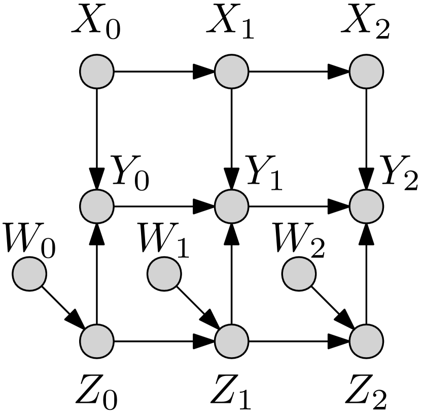
(a) Multiv.

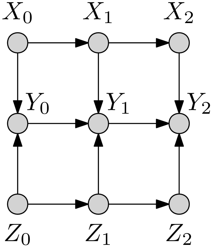
(b) Ind.

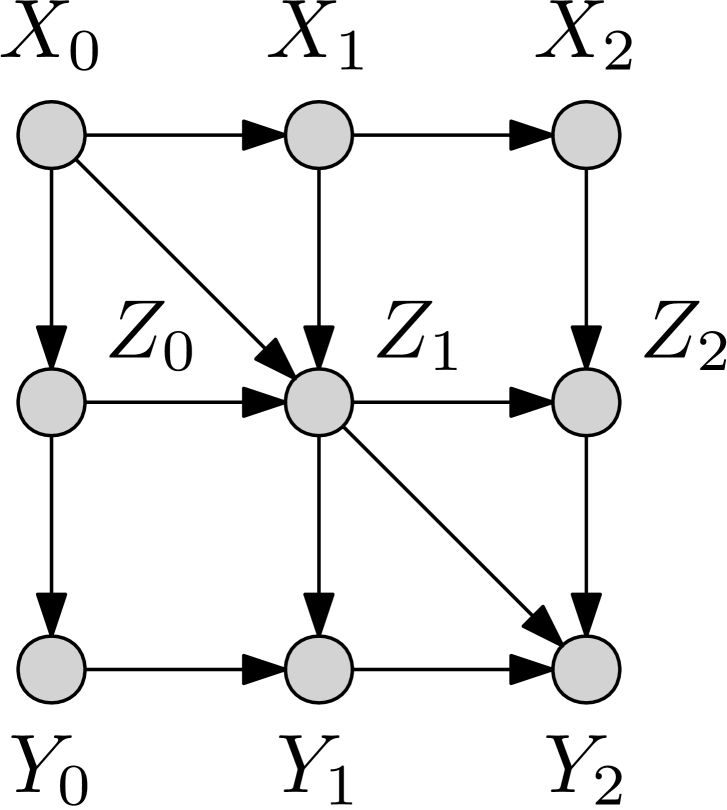
(c) NonStat.

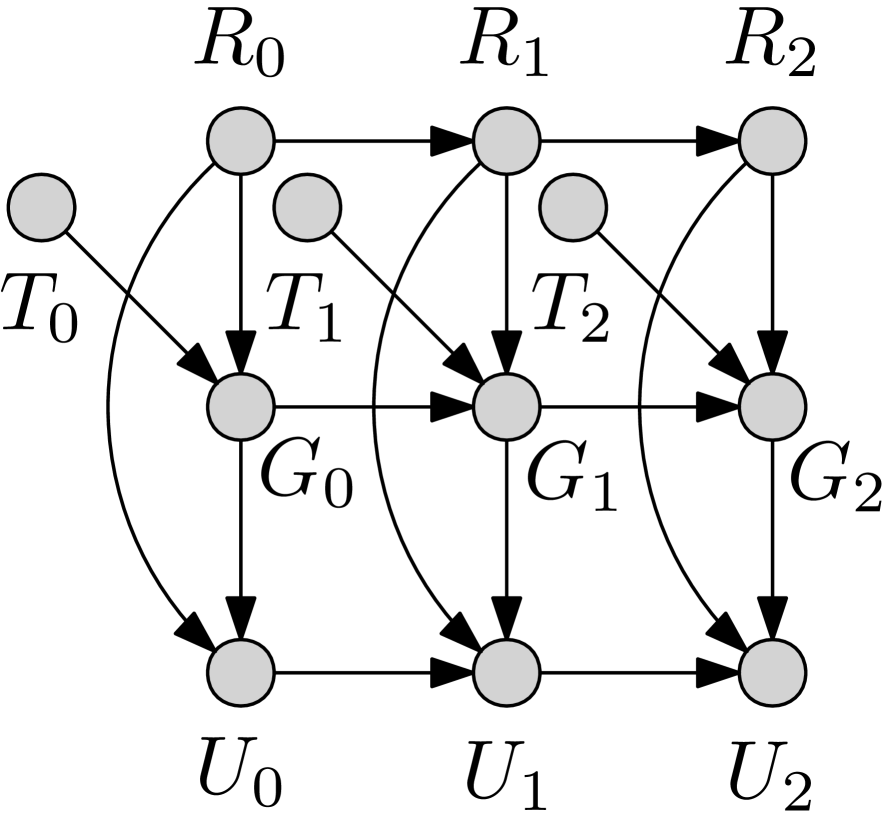
(d) Econ.

(e) ode.

Figure 3: dags used in the experimental sections for the real (Section 4.2) and synthetic data (Section 4.1).

4.1 Synthetic Experiments

Stationary dag and scm (Stat.) We run the algorithms for the dag in Fig. 1(a) with $T=3$ and $N=10$. For $t>0$, dcbo converges to the optimal value faster than competing approaches (see Fig. 6 in the supplement, right panel, 3^rd row). dcbo identifies the optimal intervention set in $93\%$ of the replicates (Table 2) and reaches the highest average gap metric (Table 1). In this experiment the location of the optimum changes significantly both in terms of optimal set and intervention value when going from $t=0$ to $t=1$. This information is incorporated by dcbo through the prior dependency on $y^{\star}_{0:t-1}$. In addition, abo performance improves over time as it accumulates interventional data and uses them to fit the temporal dimension of the surrogate model. This benefits abo in a stationary setting but might penalise it in non-stationary setting where the objective functions change significantly.

Noisy manipulative variables (Noisy): The benefit of using dcbo becomes more apparent when the manipulative variables observations are noisy while the evolution of the target variable is more accurately detected. In this case both the convergence of dcbo and cbo are slowed down by noisy observations which are diluting the information provided by the do-calculus making the priors less informative. However, the dcbo prior dependency on $y^{\star}_{0:t-1}$ allows it to correctly identify the shift in the target variable thus improving the prior accuracy and the speed-up of the algorithm (Fig. 4).

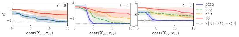
Figure 4: Experiment Noisy. Convergence of dcbo and competing methods across replicates. The dashed black line (- - -) gives the optimal outcome $y^{*}_{t},\forall t$. Shaded areas are $\pm$ one standard deviation.

Missing observational data (Miss.) Incorporating dynamic information in the surrogate model allows us to efficiently optimise a target variable even in setting where observational data are missing. We consider the dag in Fig. 1(a) with $T=6$, $N=10$ for the first three time steps and $N=0$ afterwards. dcbo uses the observational distributions learned with data from the first three time steps to construct the prior for $t>3$. On the contrary, cbo uses the standard prior for $t>3$. In this setting dcbo consistently outperforms cbo at every time step. However, abo performance improves over time and outperforms dcbo starting from $t=4$ due to its ability to exploit all interventional data collected over time (see Fig. 7 in the supplement).

Multivariate intervention sets (Multiv.) When the optimal intervention set is multivariate, both dcbo and cbo convergence speed worsen. For instance, for the dag in Fig. 3(a), $|\mathbb{M}|=5$ thus both cbo and dcbo will have to perform more explorative interventions before finding the optimum. At the same time, abo and bo consider interventions only on $\{W_{t},X_{t},Z_{t}\},\forall t$ and need to explore an even higher intervention space. The performance of all methods decrease in this case (Table 1) but dcbo still identifies the optimal intervention set in $93\%$ of the replicates (Table 2).

Independent manipulative variables (Ind.): Having to explore multiple intervention sets significantly penalises dcbo and cbo when there is no causal relationship among manipulative variables which are also the only parents of the target. This is the case for the dag in Fig. 3(b) where the optimal intervention is $\{X_{t},Z_{t}\}$ at every time step. In this case, exploring $\mathbb{M}$ and propagating uncertainty in the causal prior slows down dcbo convergence and decreases both its performance (Table 1) and capability to identify the optimal intervention set (Table 2).

Non-stationary dag and scm (NonStat.): dcbo outperforms all approaches in non-stationary settings where both the dag and the scm change overtime – see Fig. 3(c). Indeed, dcbo can timely incorporate changes in the system via the dynamic causal prior construction while cbo, bo and abo need to perform several interventions before accurately learning the new objective functions.

Table 1: Average $\textsc{g}_{t}$ across 10 replicates and time steps. See Fig. 1 for a summary of the baselines. Higher values are better. The best result for each experiment in bold. Standard errors in brackets.

	Synthetic data						Real data
	Stat.	Miss.	Noisy	Multiv.	Ind.	NonStat.	Econ.	ode
dcbo	0.88	0.84	0.75	0.49	0.48	0.69	0.64	0.67
	(0.00)	(0.01)	(0.00)	(0.01)	(0.04)	(0.00)	(0.01)	(0.00)
cbo	0.70	0.70	0.51	0.48	0.47	0.61	0.61	0.65
	(0.01)	(0.02)	(0.02)	(0.09)	(0.07)	(0.00)	(0.01)	(0.00)
abo	0.56	0.49	0.49	0.39	0.54	0.38	0.57	0.48
	(0.01)	(0.02)	(0.04)	(0.21)	(0.01)	(0.02)	(0.02)	(0.01)
bo	0.54	0.48	0.38	0.35	0.50	0.38	0.50	0.44
	(0.02)	(0.03)	(0.05)	(0.08)	(0.01)	(0.03)	(0.01)	(0.03)

Table 2: Average % of replicates across time steps for which $\mathbf{X}_{s,t}^{\star}$ is identified. See Fig. 1 for a summary of the baselines. Higher values are better. The best result for each experiment in bold.

	Synthetic data						Real data
	Stat.	Miss.	Noisy	Multiv.	Ind.	NonStat.	Econ.	ode
dcbo	93.00	58.00	100.00	93.00	93.00	100.00	86.67	33.3
cbo	90.00	85.00	90.00	90.0	90.00	100.00	93.33	33.3
abo	0.00	0.00	0.00	0.00	100.00	0.00	66.67	0.00
bo	0.00	0.00	0.00	0.00	100.00	0.00	66.67	0.00

4.2 Real experiments

Real-World Economic data (Econ.) We use dcbo to minimize the unemployment rate $U_{t}$ of a closed economy. We consider its causal relationships with economic growth ($G_{t}$), inflation rate ($R_{t}$) and fiscal policy ($T_{t}$). Inspired by the economic example in [28] we consider the dag in Fig. 3(d) where $R_{t}$ and $T_{t}$ are considered manipulative variables we need to intervene on to minimize $\log(U_{t})$ at every time step. Time series data for 10 countries are used to construct a non-parametric simulator and to compute the causal prior for both dcbo and cbo. dcbo convergences to the optimal intervention faster than competing approaches (see Table 1 and Fig. 10 in the appendix). The optimal sequence of interventions found in this experiment is equal to $\{(T_{0},R_{0})=(9.38,-2.00),(T_{1},R_{1})=(0.53,6.00),(T_{2})=(0.012)\}$ which is consistent with domain knowledge.

Planktonic predator–prey community in a chemostat (ode) We investigate a biological system in which two species interact, one as a predator and the other as prey, with the goal of identifying the intervention reducing the concentration of dead animals in the chemostat – see $D_{t}$ in Fig. 3(e). We use the system of ordinary differential equations (ode) given by [8] as our scm and construct the dag by rolling out the temporal variable dependencies in the ode while removing graph cycles. Observational data are provided in [8] and are use to compute the dynamic causal prior. dcbo outperforms competing methods in term of average gap metric and identifies the optimum faster (Table 1). Additional details can be found in the supplement (Appendix F).

5 Conclusions

We consider the problem of finding a sequence of optimal interventions in a causal graph where causal temporal dependencies exist between variables. We propose the Dynamic Causal Bayesian Optimization (dcbo) algorithm which finds the optimal intervention at every time step by intervening in the system according to a causal acquisition function. Importantly, for each possible intervention we propose to use a surrogate model that incorporates information from previous interventions implemented in the system. This is constructed by exploiting theoretical results establishing the correlation structure among objective functions for two consecutive time steps as a function of the topology of the causal graph. We discuss the dcbo performance in a variety of setting characterized by different dag properties and stationarity assumptions. Future work will focus on extending our theoretical results to more general dag structures thus allowing for unobserved confounders and a changing dag topology within each time step. In addition, we will work on combining the proposed framework with a causal discovery algorithm so as to account for uncertainty in the graph structure.

Supplementary material for
Dynamic Causal Bayesian Optimisation A Nomenclature

Symbol		Description
$\mathbf{V}_{t}$		Set of observable variables at time $t$
$\mathbf{V}_{0:T}$		Union of observable variables at time $t=0,\dots,T$
$\mathbf{X}_{t}$		Manipulative variables at time $t$
$Y_{t}$		Target variable at time $t$
$\mathcal{P}(\mathbf{X}_{t})$		Power set of $\mathbf{X}_{t}$
$\mathbb{M}_{t}$		Set of mis sets at time $t$
$\mathbf{X}_{s,t}$		$s$-th intervention set at time $t$
$\mathcal{D}$		Observational dataset $\{\mathbf{V}^{i}_{0:T}\}_{i=1}^{N}$
$N$		Number of observational data points collected from the system
$\mathcal{D}^{I}_{s,t}$		Interventional data points collected for the intervention set $\mathbf{X}_{s,t}$
$\mathbf{X}^{I}$		Vector of interventional values
$\mathbf{Y}^{I}_{s,t}$		Vector of target values obtained by intervening on $\mathbf{X}_{s,t}$ at $\mathbf{X}^{I}$
$H$		Maximum number of explorative interventions an agent can conduct at every $t$
$I_{0:t-1}$		Decision Interventions at time step $0$ to $t-1$
$f_{s,t}$		Objective function for the set $\mathbf{X}_{s,t}$
$m_{s,t}$		Prior mean function of gp on $f_{s,t}$
$k_{s,t}$		Prior kernel function of gp on $f_{s,t}$
$m_{s,t}(\cdot\mid\mathcal{D}^{I}_{s,t})$		Posterior mean function for gp on $f_{s,t}$
$k_{s,t}(\cdot,\cdot\mid\mathcal{D}^{I}_{s,t})$		Posterior covariance function for gp on $f_{s,t}$

Supplementary material for
Dynamic Causal Bayesian Optimisation B Characterization of the time structure in a dag with time dependent variables

In this section we give the proof for Theorem 1 in the main text. Consider the objective function $\mathbb{E}{\left[Y_{t}|\operatorname{do}\!\left(\mathbf{X}_{s,t}=\mathbf{x}_{s,t}\right),I_{0:t-1}\right]}$ and define the following sets:

• $\text{Pa}\!\left(Y_{t}\right)=Y_{t}^{\textsc{PT}}\cup Y_{t}^{\textsc{PNT}}$ with $Y_{t}^{\textsc{PT}}=\text{Pa}\!\left(Y_{t}\right)\cap Y_{0:t-1}$ denoting the parents of $Y_{t}$ that are target variables at previous time steps and $Y_{t}^{\textsc{PNT}}=\text{Pa}\!\left(Y_{t}\right)\backslash Y_{t}^{\textsc{PT}}$ including the parents of $Y_{t}$ that are not target variables.

• For any set $\mathbf{X}_{s,t}\in\mathcal{P}(\mathbf{X}_{t})$, $\mathbf{X}_{s,t}^{\textsc{PY}}=\mathbf{X}_{s,t}\cap\text{Pa}\!\left(Y_{t}\right)$ includes the variables in $\mathbf{X}_{s,t}$ that are parents of $Y_{t}$ while $\mathbf{X}_{s,t}^{\textsc{NPY}}=\mathbf{X}_{s,t}\backslash\mathbf{X}_{s,t}^{\textsc{PY}}$ so that $\mathbf{X}_{s,t}=\mathbf{X}_{s,t}^{\textsc{PY}}\cup\mathbf{X}_{s,t}^{\textsc{NPY}}$.

• For any set $I_{0:t-1}^{V}\subseteq\mathbf{X}_{0:t-1}$, $I_{0:t-1}^{\textsc{PY}}=I_{0:t-1}^{V}\cap\text{Pa}\!\left(Y_{t}\right)$ includes the variables in $I_{0:t-1}^{V}$ that are parents of $Y_{t}$ and $I_{0:t-1}^{\textsc{NPY}}=I_{0:t-1}^{V}\backslash I_{0:t-1}^{\textsc{PY}}$ so that $I_{0:t-1}^{V}=I_{0:t-1}^{\textsc{PY}}\cup I_{0:t-1}^{\textsc{NPY}}$.

• For any two sets $\mathbf{X}_{s,t}\in\text{Pa}\!\left(Y_{t}\right)$ and $I_{0:t-1}^{V}\subseteq\mathbf{X}_{0:t-1}$, $\mathbf{W}$ is a set such that $\text{Pa}\!\left(Y_{t}\right)=Y_{t}^{\textsc{PT}}\cup\mathbf{X}_{s,t}^{\textsc{PY}}\cup I_{0:t-1}^{\textsc{PY}}\cup\mathbf{W}$. This means that $\mathbf{W}$ includes those variables that are parents of $Y_{t}$ but are nor target at previous time steps nor intervened variables.

In the following proof the values of $I_{0:t-1}^{V}$, $\mathbf{X}_{s,t}^{\textsc{PY}}$, $I_{0:t-1}^{\textsc{PY}}$ and $W$ are denoted by $\mathbf{i}$, $\mathbf{x}^{\textsc{PY}}$, $\mathbf{i}^{\textsc{PY}}$ and $\mathbf{w}$ respectively. The values of $Y_{t}^{\textsc{PT}}$, $\mathbf{X}_{s,t}^{\textsc{NPY}}$ and $I_{0:t-1}^{\textsc{NPY}}$ are instead represented by $\mathbf{y}_{t}^{\textsc{PT}}$, $\mathbf{x}^{\textsc{NPY}}$ and $\mathbf{i}^{\textsc{NPY}}$. Finally, $f_{Y}^{Y}$ and $f_{Y}^{\text{NY}}$ are the functions in the scm for $Y_{t}$ (see Assumptions (1) in the main text).

Proof of Theorem 1

Under Assumptions 1 we can write :

$$\mathbb{E}{\left[Y_{t}|\operatorname{do}\!\left(\mathbf{X}_{s,t}=\mathbf{x}_{s,t}\right),I_{0:t-1}\right]} =\int y_{t}p(y_{t}|\operatorname{do}\!\left(\mathbf{X}_{s,t}=\mathbf{x}_{s,t}\right),I_{0:t-1})\text{d}y_{t}$$

$$=\int\cdots\int y_{t}p(y_{t}|\operatorname{do}\!\left(\mathbf{X}_{s,t}^{\textsc{PY}}=\mathbf{x}^{\textsc{PY}}\right),\operatorname{do}\!\left(\mathbf{X}_{s,t}^{\textsc{NPY}}=\mathbf{x}^{\textsc{NPY}}\right),I_{0:t-1}^{\textsc{PY}},I_{0:t-1}^{\textsc{NPY}},\mathbf{y}_{t}^{\textsc{PT}},\mathbf{w})$$

$$\;\;\;\;\;\;\;\;\;\;\;\;\;\;\;\;\times p(\mathbf{y}_{t}^{\textsc{PT}},\mathbf{w}|\operatorname{do}\!\left(\mathbf{X}_{s,t}=\mathbf{x}_{s,t}\right),I_{0:t-1})\text{d}y_{t}\text{d}\mathbf{y}_{t}^{\textsc{PT}}\text{d}\mathbf{w}$$

$$=\Big{/}\text{Rule 2 and Rule 1 of do-calculus}\Big{/}$$

$$=\int\cdots\int y_{t}p(y_{t}|\operatorname{do}\!\left(\mathbf{X}_{s,t}^{\textsc{PY}}=\mathbf{x}^{\textsc{PY}}\right),I_{0:t-1}^{\textsc{PY}},\mathbf{y}_{t}^{\textsc{PT}},\mathbf{w})$$

$$\;\;\;\;\;\;\;\;\;\;\;\;\;\;\;\;\times p(\mathbf{y}_{t}^{\textsc{PT}},\mathbf{w}|\operatorname{do}\!\left(\mathbf{X}_{s,t}=\mathbf{x}_{s,t}\right),I_{0:t-1})\text{d}y_{t}\text{d}\mathbf{y}_{t}^{\textsc{PT}}\text{d}\mathbf{w}$$ (5)

$$=\int\cdots\int\mathbb{E}{\left[Y_{t}|\operatorname{do}\!\left(\mathbf{X}_{s,t}^{\textsc{PY}}=\mathbf{x}^{\textsc{PY}}\right),I_{0:t-1}^{\textsc{PY}},\mathbf{y}_{t}^{\textsc{PT}},\mathbf{w}\right]}$$

$$\;\;\;\;\;\;\;\;\;\;\;\;\;\;\;\;\times p(\mathbf{y}_{t}^{\textsc{PT}},\mathbf{w}|\operatorname{do}\!\left(\mathbf{X}_{s,t}=\mathbf{x}_{s,t}\right),I_{0:t-1})\text{d}\mathbf{y}_{t}^{\textsc{PT}}\text{d}\mathbf{w}$$

$$=\Big{/}\text{Assumption (2)}\Big{/}$$

$$=\int\cdots\int f_{Y}^{Y}(\mathbf{y}_{t}^{\textsc{PT}})+f_{Y}^{\text{NY}}(\mathbf{x}^{\textsc{PY}},\mathbf{i}^{\textsc{PY}},\mathbf{w})$$

$$\;\;\;\;\;\;\;\;\;\;\;\;\;\;\;\;\times p(\mathbf{y}_{t}^{\textsc{PT}},\mathbf{w}|\operatorname{do}\!\left(\mathbf{X}_{s,t}=\mathbf{x}_{s,t}\right),I_{0:t-1})\text{d}\mathbf{y}_{t}^{\textsc{PT}}\text{d}\mathbf{w}$$ (6)

$$=\int\cdots\int f_{Y}^{Y}(\mathbf{y}_{t}^{\textsc{PT}})p(\mathbf{y}_{t}^{\textsc{PT}},\mathbf{w}|\operatorname{do}\!\left(\mathbf{X}_{s,t}=\mathbf{x}_{s,t}\right),I_{0:t-1})\text{d}\mathbf{y}_{t}^{\textsc{PT}}\text{d}\mathbf{w}$$

$$+\int\cdots\int f_{Y}^{\text{NY}}(\mathbf{x}^{\textsc{PY}},\mathbf{i}^{\textsc{PY}},\mathbf{w})p(\mathbf{y}_{t}^{\textsc{PT}},\mathbf{w}|\operatorname{do}\!\left(\mathbf{X}_{s,t}=\mathbf{x}_{s,t}\right),I_{0:t-1})\text{d}\mathbf{y}_{t}^{\textsc{PT}}\text{d}\mathbf{w}$$

$$=\int f_{Y}^{Y}(\mathbf{y}_{t}^{\textsc{PT}})p(\mathbf{y}_{t}^{\textsc{PT}}|\operatorname{do}\!\left(\mathbf{X}_{s,t}=\mathbf{x}_{s,t}\right),I_{0:t-1})\text{d}\mathbf{y}_{t}^{\textsc{PT}}$$ (7)

$$+\int f_{Y}^{\text{NY}}(\mathbf{x}^{\textsc{PY}},\mathbf{i}^{\textsc{PY}},\mathbf{w})p(\mathbf{w}|\operatorname{do}\!\left(\mathbf{X}_{s,t}=\mathbf{x}_{s,t}\right),I_{0:t-1})\text{d}\mathbf{w}$$

$$=\Big{/}\text{Time assumption}\Big{/}$$

$$=\int f_{Y}^{Y}(\mathbf{y}_{t}^{\textsc{PT}})p(\mathbf{y}_{t}^{\textsc{PT}}|I_{0:t-1})\text{d}\mathbf{y}_{t}^{\textsc{PT}}+\int f_{Y}^{\text{NY}}(\mathbf{x}^{\textsc{PY}},\mathbf{i}^{\textsc{PY}},\mathbf{w})p(\mathbf{w}|\operatorname{do}\!\left(\mathbf{X}_{s,t}=\mathbf{x}_{s,t}\right),I_{0:t-1})\text{d}\mathbf{w}$$ (8)

$$=\Big{/}\text{Observed interventions}\Big{/}$$

$$=f_{Y}^{Y}(\mathbf{f}^{\star})+\int f_{Y}^{\text{NY}}(\mathbf{x}^{\textsc{PY}},\mathbf{i}^{\textsc{PY}},\mathbf{w})p(\mathbf{w}|\operatorname{do}\!\left(\mathbf{X}_{s,t}=\mathbf{x}_{s,t}\right),I_{0:t-1})\text{d}\mathbf{w}$$ (9)

$$=f_{Y}^{Y}(\mathbf{f}^{\star})+\mathbb{E}_{p(\mathbf{w}|\operatorname{do}\!\left(\mathbf{X}_{s,t}=\mathbf{x}_{s,t}\right),I_{0:t-1})}{\left[f_{Y}^{\text{NY}}(\mathbf{x}^{\textsc{PY}},\mathbf{i}^{\textsc{PY}},\mathbf{w})\right]}$$ (10)

with $\mathbf{f}^{\star}=\{\mathbb{E}{\left[Y_{i}|\operatorname{do}\!\left(\mathbf{X}_{s,i}^{\star}=\mathbf{x}_{s,i}^{\star}\right),I_{0:i-1}\right]}\}_{Y_{i}\in Y_{t}^{\textsc{PT}}}$ denoting the values of $Y_{t}^{\textsc{PT}}$ corresponding to the optimal interventions implemented at previous time steps . Eq. (5) follows from $Y_{t}\rotatebox[origin={c}]{90.0}{$\models$}(\mathbf{X}_{s,t}^{\textsc{NPY}}\cup I_{0:t-1}^{\textsc{NPY}})|\mathbf{X}_{s,t}^{\textsc{PY}},I_{0:t-1}^{\textsc{PY}},\mathbf{W},Y_{t}^{\textsc{PT}}\;\;\text{in}\;\;\mathcal{G}_{\overline{\mathbf{X}_{s,t}^{\textsc{PY}},I_{0:t-1}^{\textsc{PY}}}\underline{\mathbf{X}_{s,t}^{\textsc{NPY}},I_{0:t-1}^{\textsc{NPY}}}}$ (Rule 2 of do-calculus) and $Y_{t}\rotatebox[origin={c}]{90.0}{$\models$}(\mathbf{X}_{s,t}^{\textsc{NPY}}\cup I_{0:t-1}^{\textsc{NPY}})|\mathbf{X}_{s,t}^{\textsc{PY}},I_{0:t-1}^{\textsc{PY}},\mathbf{W},Y_{t}^{\textsc{PT}}\;\;\text{in}\;\;\mathcal{G}_{\overline{\mathbf{X}_{s,t}^{\textsc{PY}},I_{0:t-1}^{\textsc{PY}}}}$ (Rule 1 of do-calculus). Eq. (6) follows from the second assumption in Assumptions (1) in the main text. Eq. (8) follows from $Y_{t}^{\textsc{PT}}\rotatebox[origin={c}]{90.0}{$\models$}\mathbf{X}_{s,t}$ as interventions at time $t$ cannot affect variables at time steps $0:t-1$. Finally, noticing that $p(\mathbf{y}_{t}^{\textsc{PT}}|I_{0:t-1})$ is the distribution targeted when optimizing the objective function at previous time steps one can obtain Eq. (10).

$\blacksquare$

The derivations above show how the objective function at time $t$ is given by the expected value of the output of the functional relationship $f_{Y}^{\text{NY}}$ where the expectation is taken with respect to the variables that are not intervened on. This expectation is then shifted to account for the interventions implemented in the system at previous time steps that are affecting the target variable through $f_{Y}^{Y}$. Notice that, given our assumption on the absence of unobserved confounders, the distribution $p(\mathbf{w}|\operatorname{do}\!\left(\mathbf{X}_{s,t}=\mathbf{x}_{s,t}\right),I_{0:t-1})$ can be further simplified by conditioning on the variables in $\mathcal{G}$ that are on the back-door path between $(\mathbf{X}_{s,t},I_{0:t-1})$ and $Y_{t}$ and are not colliders. When the variable $Y_{t}$ does not depend on the previous target nodes, the function $f_{Y}^{Y}$ does not exist and Eq. (10) reduces to

$$\mathbb{E}_{p(\mathbf{w}|\operatorname{do}\!\left(\mathbf{X}_{s,t}=\mathbf{x}_{s,t}\right),I_{0:t-1})}{\left[f_{Y}^{\text{NY}}(\mathbf{x}^{\textsc{PY}},\mathbf{i}^{\textsc{PY}},\mathbf{w})\right]}.$$ (11)

In this case previous interventions impact the target variable at time $t$ by changing the distributions of the parents of $Y_{t}$ that are not intervened but the information in $\mathbf{f}^{\star}$ is lost.

Eq. (10) can be further manipulated to reduce the second term to a do-free expression. Instead of applying the rules of do-calculus, one can expand $p(\mathbf{w}|\operatorname{do}\!\left(\mathbf{X}_{s,t}=\mathbf{x}_{s,t}\right),I_{0:t-1})$ by further conditioning on the parents of $\mathbf{W}$ that are not in $(\mathbf{X}_{s,t}\cup I_{0:t-1})$. In this case, $\mathbf{w}$ in $f_{Y}^{\text{NY}}(\mathbf{x}^{\textsc{PY}},\mathbf{i}^{\textsc{PY}},\mathbf{w})$ is replaced by the functions $\{f_{W}(\cdot)\}_{W\in\mathbf{W}}$ in the scm corresponding to the variables in $\mathbf{W}$ and computed in $\mathbf{w}$. This leads to a partial composition of $f_{Y}^{\text{NY}}$ with $\{f_{W}(\cdot)\}_{W\in\mathbf{W}}$ and can be repeated recursively until the set of variables with respect to which we are taking the expectation is a subset of $\mathbf{X}_{s,t}$ or $I_{0:t-1}^{V}$ thus making the distribution a delta function. For instance, when $\mathbf{W}\subset\mathbf{X}_{s,t}$ in Eq. (10), we have $p(\mathbf{w}|\operatorname{do}\!\left(\mathbf{X}_{s,t}=\mathbf{x}_{s,t}\right),I_{0:t-1})=\delta(\mathbf{w}=\mathbf{x}^{\textsc{W}}))$ where $\mathbf{x}^{\textsc{W}}$ are the values in $\mathbf{x}_{s,t}$ corresponding to the variables in $\mathbf{W}$. Therefore, Eq. (10) reduces to $f_{Y}^{Y}(\mathbf{f}^{\star})+{f_{Y}^{\text{NY}}(\mathbf{x}^{\textsc{PY}},\mathbf{i}^{\textsc{PY}},\mathbf{x}^{\textsc{W}})}$.

For a generic $W\in\mathbf{W}\not\subseteq(\mathbf{X}_{s,t}\cup I_{0:t-1}^{V})$, denote by $\mathbf{X}_{s,t}^{\textsc{PW}}$ and $I_{0:t-1}^{\textsc{PW}}$ the subset of variables in $\mathbf{X}_{s,t}$ and $I_{0:t-1}$ that are parents of $W$ with corresponding values $\mathbf{x}^{\textsc{PW}}$ and $\mathbf{i}^{\textsc{PW}}$. Let $R=\text{Pa}\!\left(W\right)\backslash(\mathbf{X}_{s,t}^{\textsc{PW}}\cup I_{0:t-1}^{\textsc{PW}})$ and $r$ be the corresponding value. We can define the $C(\cdot)$ function as:

$$C(W)=\begin{cases}f_{W}(\mathbf{u}_{W},\mathbf{x}^{\textsc{PW}},\mathbf{i}^{\textsc{PW}})&\quad\text{if}\quad R=\varnothing\\ f_{W}(\mathbf{u}_{W},\mathbf{x}^{\textsc{PW}},\mathbf{i}^{\textsc{PW}},r)&\quad\text{if}\quad R\subseteq\mathbf{X}_{s,t}\cup I_{0:t-1}^{V}\\ f_{W}(\mathbf{u}_{W},\mathbf{x}^{\textsc{PW}},\mathbf{i}^{\textsc{PW}},C(R))&\quad\text{if}\quad R\not\subseteq\mathbf{X}_{s,t}\cup I_{0:t-1}^{V}\end{cases}$$ (12)

with $u_{W}$ representing the exogenous variables with edges into $W$ and $f_{W}$ denoting the functional mapping for $W$ in the scm. Note that if $R=\varnothing$ and $\mathbf{X}_{s,t}^{\textsc{PW}}$ and $I_{0:t-1}^{\textsc{PW}}$ are also empty then $f_{W}(\mathbf{u}_{W},\mathbf{x}^{\textsc{PW}},\mathbf{i}^{\textsc{PW}})$ reduces to $f_{W}(\mathbf{u}_{W})$. The same holds for the other cases that is $f_{W}(\mathbf{u}_{W},\mathbf{x}^{\textsc{PW}},\mathbf{i}^{\textsc{PW}},r)=f_{W}(\mathbf{u}_{W},r)$ and $f_{W}(\mathbf{u}_{W},\mathbf{x}^{\textsc{PW}},\mathbf{i}^{\textsc{PW}},C(R))=f_{W}(\mathbf{u}_{W},C(R))$ when $\mathbf{X}_{s,t}^{\textsc{PW}},I_{0:t-1}^{\textsc{PW}}=\varnothing$. Exploiting Eq. (12) we can rewrite Eq. (10) as:

$$\mathbb{E}{\left[Y_{t}|\operatorname{do}\!\left(\mathbf{X}_{s,t}=\mathbf{x}_{s,t}\right),I_{0:t-1}\right]} =f_{Y}^{Y}(\mathbf{f}^{\star})+\mathbb{E}_{p(\mathbf{U}_{0:t})}{\left[f_{Y}^{\text{NY}}(\mathbf{x}^{\textsc{PY}},\mathbf{i}^{\textsc{PY}},\{C(W)\}_{W\in\mathbf{W}})\right]}$$ (13)

The distribution $p(\mathbf{U}_{0:t})$ can be further simplified to consider only the exogenous variables with outgoing edges into the variables on the directed paths between $\mathbf{X}_{s,t}$ and $Y_{t}^{\textsc{PNT}}$ and between $I_{0:t-1}^{V}$ and $Y_{t}^{\textsc{PNT}}$. Notice how the second term in Eq. (13) propagates the interventions, both at the present and past time steps, through the scm so as to express the parents of the target variable as a function of the intervened values. The expected target is then obtained as the propagation of the intervened variables and intervened targets through the function $f_{Y_{t}}$ in the scm.

Supplementary material for
Dynamic Causal Bayesian Optimisation C Example derivations

Next we show how one can use Theorem 1 to derive some of the objective functions used by dcbo for the dags in Fig. 5.

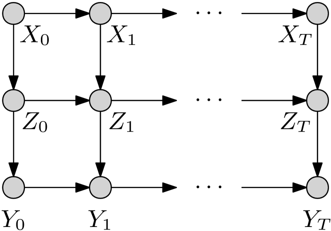
(a) dag 1

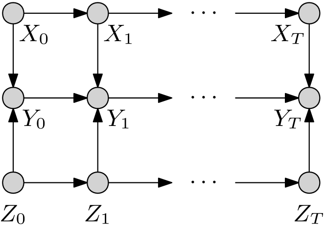
(b) dag 2

Figure 5: Dynamic Bayesian networks with different topologies. Figure 5(a) shows a dag in which (per time-slice) the manipulative variable $X$ flows through $Z$, whereas in Fig. 5(b) the manipulative variables are independent of each other (note the direction of the vertical edges).

C.1 Derivations for dag 1 in Fig. 5(a)

Consider the dag in Fig. 5(a) and assume that the optimal intervention implemented at time $t=0$ is given by $I_{0}=\operatorname{do}\!\left(Z_{0}=z_{0}^{\star}\right)$ and gives a target value of $y_{0}^{\star}$. At $t=1$ the target variable is $Y_{1}$, $Y_{t}^{\textsc{PT}}=\{Y_{0}\}$ and $Y_{t}^{\textsc{PNT}}=\{Z_{1}\}$. Given $I_{0}$ we have $I_{0:t-1}^{\textsc{PY}}=\varnothing$ and $I_{0:t-1}^{\textsc{NPY}}=Z_{0}$. We can write the objective functions by noticing that, for $\mathbf{X}_{s,1}=\{Z_{1}\}$ we have $\mathbf{X}_{s,t}^{\textsc{PY}}=\{Z_{1}\}$, $\mathbf{X}_{s,t}^{\textsc{NPY}}=\varnothing$ and $W=\varnothing$, while for $\mathbf{X}_{s,1}=\{X_{1}\}$ we have $\mathbf{X}_{s,t}^{\textsc{PY}}=\varnothing$, $\mathbf{X}_{s,t}^{\textsc{NPY}}=\{X_{1}\}$ and $W=\{Z_{1}\}$. We do not compute the objective function for $\mathbf{X}_{s,1}=\{X_{1},Z_{1}\}$ as this is equal to the function for $\mathbf{X}_{s,1}=\{Z_{1}\}$. Starting with $\mathbf{X}_{s,1}=\{Z_{1}\}$ we have:

$$\mathbb{E}{\left[Y_{1}|\operatorname{do}\!\left(Z_{1}=z\right),I_{0}\right]} =\int y_{1}p(y_{1}|\operatorname{do}\!\left(Z_{1}=z\right),I_{0})\text{d}y_{1}$$

$$=\int\int y_{1}p(y_{1}|y_{0},\operatorname{do}\!\left(Z_{1}=z\right),I_{0})p(y_{0}|\operatorname{do}\!\left(Z_{1}=z\right),I_{0})\text{d}y_{1}\text{d}y_{0}$$

$$=\int\mathbb{E}{\left[Y_{1}|y_{0},\operatorname{do}\!\left(Z_{1}=z\right)\right]}p(y_{0}|\operatorname{do}\!\left(Z_{1}=z\right),I_{0})\text{d}y_{0}$$

$$=\int[f_{Y}^{Y}(y_{0})+f_{Y}^{\text{NY}}(z)]p(y_{0}|I_{0})\text{d}y_{0}$$

$$=\int f_{Y}^{Y}(y_{0})p(y_{0}|I_{0})\text{d}y_{0}+f_{Y}^{\text{NY}}(z)$$

$$=f_{Y}^{Y}(y_{0}^{\star})+f_{Y}^{\text{NY}}(z)$$

Notice that here $\mathbf{X}_{s,t}^{\textsc{PY}}=\{Z_{1}\}$, $I_{0:t-1}^{\textsc{PY}}=\varnothing$ and $W=\varnothing$ thus $\mathbb{E}_{p(\mathbf{w}|\operatorname{do}\!\left(\mathbf{X}_{s,t}=\mathbf{x}_{s,t}\right),I_{0:t-1})}{\left[f_{Y}^{\text{NY}}(\mathbf{x}^{\textsc{PY}},\mathbf{i}^{\textsc{PY}},\mathbf{w})\right]}=f_{Y}^{\text{NY}}(z)$. The objective function for $\mathbf{X}_{s,1}=\{X_{1}\}$ can be written as:

$$\mathbb{E}{\left[Y_{1}|\operatorname{do}\!\left(X_{1}=x\right),I_{0}\right]} =\int y_{1}p(y_{1}|\operatorname{do}\!\left(X_{1}=x\right),I_{0})\text{d}y_{1}$$

$$=\int\int\int y_{1}p(y_{1}|y_{0},z_{1},\operatorname{do}\!\left(X_{1}=x\right),I_{0})p(y_{0},z_{1}|\operatorname{do}\!\left(X_{1}=x\right),I_{0})\text{d}y_{1}\text{d}y_{0}\text{d}z_{1}$$

$$=\int\int\int y_{1}p(y_{1}|y_{0},z_{1})p(y_{0},z_{1}|\operatorname{do}\!\left(X_{1}=x\right),I_{0})\text{d}y_{1}\text{d}y_{0}\text{d}z_{1}$$

$$=\int\int\mathbb{E}{\left[Y_{1}|y_{0},z_{1}\right]}p(y_{0},z_{1}|\operatorname{do}\!\left(X_{1}=x\right),I_{0})\text{d}y_{0}\text{d}z_{1}$$

$$=\int\int[f_{Y}^{Y}(y_{0})+f_{Y}^{\text{NY}}(z_{1})]p(y_{0},z_{1}|\operatorname{do}\!\left(X_{1}=x\right),I_{0})\text{d}y_{0}\text{d}z_{1}$$

$$=\int\int f_{Y}^{Y}(y_{0})p(y_{0},z_{1}|\operatorname{do}\!\left(X_{1}=x\right),I_{0})\text{d}y_{0}\text{d}z_{1}$$ (14)

$$+\int\int f_{Y}^{\text{NY}}(z_{1})p(y_{0},z_{1}|\operatorname{do}\!\left(X_{1}=x\right),I_{0})\text{d}y_{0}\text{d}z_{1}$$

$$=\int f_{Y}^{Y}(y_{0})p(y_{0}|I_{0})\text{d}y_{0}+\int\int f_{Y}^{\text{NY}}(z_{1})p(z_{1}|\operatorname{do}\!\left(X_{1}=x\right),I_{0})\text{d}z_{1}$$

$$=f_{Y}^{Y}(y_{0}^{\star})+\int f_{Y}^{\text{NY}}(z_{1})p(z_{1}|\operatorname{do}\!\left(X_{1}=x\right),I_{0})\text{d}z_{1}$$ (15)

In this case $\mathbf{X}_{s,t}^{\textsc{PY}}=\varnothing$, $I_{0:t-1}^{\textsc{PY}}=\varnothing$ and $\mathbf{W}=\{Z_{1}\}$ thus

$$\mathbb{E}_{p(\mathbf{w}|\operatorname{do}\!\left(\mathbf{X}_{s,t}=\mathbf{x}_{s,t}\right),I_{0:t-1})}{\left[f_{Y}^{\text{NY}}(\mathbf{x}^{\textsc{PY}},\mathbf{i}^{\textsc{PY}},\mathbf{w})\right]}=\mathbb{E}_{p(z_{1}|\text{do}(X_{1}=x),I_{0})}{\left[f_{Y}^{\text{NY}}(z_{1})\right]}.$$ (16)

We can further expand Eq. (15) noticing that in this case $\mathbf{W}=\{Z_{1}\}\not\subseteq\{X_{1},Z_{0}\}$ but $\mathbf{X}_{s,t}^{PW}=\{X_{1}\}$, $I_{0:t-1}^{PW}=\{Z_{0}\}$ and $R=\varnothing$. Therefore we have $C(Z_{1})=f_{Z_{1}}(\epsilon_{Z_{1}},x_{1},z_{1})$ and Eq. (15) becomes:

$$\mathbb{E}{\left[Y|\operatorname{do}\!\left(X_{1}=x\right),I_{0}\right]} =f_{Y}^{Y}(y_{0}^{\star})+\int f_{Y}^{\text{NY}}(z_{1})p(z_{1}|\operatorname{do}\!\left(X_{1}=x\right),I_{0})\text{d}z_{1}$$

$$=f_{Y}^{Y}(y_{0}^{\star})+\int\int f_{Y}^{\text{NY}}(z_{1})p(z_{1}|\epsilon_{Z_{1}},\operatorname{do}\!\left(X_{1}=x\right),I_{0})p(\epsilon_{Z_{1}}|\operatorname{do}\!\left(X_{1}=x\right),I_{0})\text{d}z_{1}\text{d}\epsilon_{Z_{1}}$$

$$=f_{Y}^{Y}(y_{0}^{\star})+\int\int f_{Y}^{\text{NY}}(z_{1})\delta(z_{1}=f_{Z_{1}}(\epsilon_{Z_{1}},x,z_{0}^{\star}))p(\epsilon_{Z_{1}})\text{d}z_{1}\text{d}\epsilon_{Z_{1}}$$

$$=f_{Y}^{Y}(y_{0}^{\star})+\mathbb{E}_{p(\epsilon_{Z_{1}})}{\left[f_{Y}^{\text{NY}}(f_{Z_{1}}(\epsilon_{Z_{1}},x,z_{0}^{\star}))\right]}.$$

C.2 Derivations for dag 2 in Fig. 5(b)

Next we consider the dag in Fig. 5(b) and assume that the optimal interventions implemented at time $t=0$ and $t=1$ are given by $I_{0}=\operatorname{do}\!\left(X_{0}=x_{0}^{\star}\right)$ and $I_{1}=\operatorname{do}\!\left(Z_{1}=z_{1}^{\star}\right)$. The optimal target values associated with these two interventions are given by $y_{0}^{\star}$ and $y_{1}^{\star}$ respectively. We are interested in computing two objective functions: $\mathbb{E}{\left[Y_{2}|\operatorname{do}\!\left(X_{2}=x_{2}\right),I_{0},I_{1}\right]}$ and $\mathbb{E}{\left[Y_{2}|\operatorname{do}\!\left(Z_{2}=z_{2}\right),I_{0},I_{1}\right]}$. In this case $\mathbf{y}_{t}^{\textsc{PT}}=\{Y_{1}\}$, $Y_{t}^{\textsc{PNT}}=\{X_{2},Z_{2}\}$, $I_{0:t-1}^{\textsc{PY}}=\varnothing$ and $I_{0:t-1}^{\textsc{NPY}}=\{X_{0},Z_{1}\}$. Starting from $\mathbb{E}{\left[Y_{2}|\operatorname{do}\!\left(X_{2}=x_{2}\right),I_{0},I_{1}\right]}$, when $\mathbf{X}_{s,2}=\{X_{2}\}$ we have $\mathbf{X}_{s,t}^{\textsc{PY}}=\{X_{2}\}$, $\mathbf{X}_{s,t}^{\textsc{NPY}}=\varnothing$ and $W=\{Z_{2}\}$. We can write:

$$\mathbb{E}{\left[Y_{2}|\operatorname{do}\!\left(X_{2}=x_{2}\right),I_{0},I_{1}\right]} =\int y_{2}p(y_{2}|\operatorname{do}\!\left(X_{2}=x_{2}\right),I_{0},I_{1})\text{d}y_{2}$$

$$=\int\int\int y_{2}p(y_{2}|y_{1},z_{2},\operatorname{do}\!\left(X_{2}=x_{2}\right),I_{0},I_{1})p(y_{1},z_{2}|\operatorname{do}\!\left(X_{2}=x_{2}\right),I_{0},I_{1})\text{d}y_{2}\text{d}y_{1}\text{d}z_{2}$$

$$=\int\int\int y_{2}p(y_{2}|y_{1},z_{2},\operatorname{do}\!\left(X_{2}=x_{2}\right))p(y_{1},z_{2}|\operatorname{do}\!\left(X_{2}=x_{2}\right),I_{0},I_{1})\text{d}y_{2}\text{d}y_{1}\text{d}z_{2}$$

$$=\int\int\mathbb{E}{\left[Y_{2}|y_{1},z_{2},\operatorname{do}\!\left(X_{2}=x_{2}\right)\right]}p(y_{1},z_{2}|\operatorname{do}\!\left(X_{2}=x_{2}\right),I_{0},I_{1})\text{d}y_{1}\text{d}z_{2}$$

$$=\int\int[f_{Y}^{Y}(y_{1})+f_{Y}^{\text{NY}}(x_{2},z_{2})]p(y_{1},z_{2}|\operatorname{do}\!\left(X_{2}=x_{2}\right),I_{0},I_{1})\text{d}y_{1}\text{d}z_{2}$$

$$=\int\int f_{Y}^{Y}(y_{1})p(y_{1},z_{2}|\operatorname{do}\!\left(X_{2}=x_{2}\right),I_{0},I_{1})\text{d}y_{1}\text{d}z_{2}$$

$$+\int\int f_{Y}^{\text{NY}}(x_{2},z_{2})p(y_{1},z_{2}|\operatorname{do}\!\left(X_{2}=x_{2}\right),I_{0},I_{1})\text{d}y_{1}\text{d}z_{2}$$

$$=\int f_{Y}^{Y}(y_{1})p(y_{1}|I_{0},I_{1})\text{d}y_{1}+\int f_{Y}^{\text{NY}}(x_{2},z_{2})p(z_{2}|\operatorname{do}\!\left(X_{2}=x_{2}\right),I_{0},I_{1})\text{d}z_{2}$$

$$=f_{Y}^{Y}(y_{1}^{\star})+\int f_{Y}^{\text{NY}}(x_{2},z_{2})p(z_{2}|I_{1})\text{d}z_{2}$$

$$=f_{Y}^{Y}(y_{1}^{\star})+\mathbb{E}_{p(\epsilon_{Z_{2}})}{\left[f_{Y}^{\text{NY}}(x_{2},f_{Z_{2}}(z_{1}^{\star},\epsilon_{Z_{2}}))\right]}$$

Next we compute $\mathbb{E}{\left[Y_{2}|\operatorname{do}\!\left(Z_{2}=z_{2}\right),I_{0},I_{1}\right]}$ by noticing that, when $\mathbf{X}_{s,2}=\{Z_{2}\}$, we have $\mathbf{X}_{s,t}^{\textsc{PY}}=\{Z_{2}\}$, $\mathbf{X}_{s,t}^{\textsc{NPY}}=\varnothing$ and $W=\{X_{2}\}$. In this case we have:

$$\mathbb{E}{\left[Y_{2}|\operatorname{do}\!\left(Z_{2}=z_{2}\right),I_{0},I_{1}\right]} =\int y_{2}p(y_{2}|\operatorname{do}\!\left(Z_{2}=z_{2}\right),I_{0},I_{1})\text{d}y_{2}$$

$$=\int\int\int y_{2}p(y_{2}|y_{1},x_{2},\operatorname{do}\!\left(Z_{2}=z_{2}\right),I_{0},I_{1})p(y_{1},x_{2}|\operatorname{do}\!\left(Z_{2}=z_{2}\right),I_{0},I_{1})\text{d}y_{2}\text{d}y_{1}\text{d}x_{2}$$

$$=\int\int\int y_{2}p(y_{2}|y_{1},x_{2},\operatorname{do}\!\left(Z_{2}=z_{2}\right))p(y_{1},x_{2}|\operatorname{do}\!\left(Z_{2}=z_{2}\right),I_{0},I_{1})\text{d}y_{2}\text{d}y_{1}\text{d}x_{2}$$

$$=\int\int\mathbb{E}{\left[Y_{2}|y_{1},x_{2},\operatorname{do}\!\left(Z_{2}=z_{2}\right)\right]}p(y_{1},x_{2}|\operatorname{do}\!\left(Z_{2}=z_{2}\right),I_{0},I_{1})\text{d}y_{1}\text{d}x_{2}$$

$$=\int\int[f_{Y}^{Y}(y_{1})+f_{Y}^{\text{NY}}(x_{2},z_{2})]p(y_{1},x_{2}|\operatorname{do}\!\left(Z_{2}=z_{2}\right),I_{0},I_{1})\text{d}y_{1}\text{d}x_{2}$$

$$=\int f_{Y}^{Y}(y_{1})p(y_{1}|I_{0},I_{1})\text{d}y_{1}+\int f_{Y}^{\text{NY}}(x_{2},z_{2})p(x_{2}|\operatorname{do}\!\left(Z_{2}=z_{2}\right),I_{0},I_{1})\text{d}x_{2}$$

$$=f_{Y}^{Y}(y_{1}^{\star})+\int f_{Y}^{\text{NY}}(x_{2},z_{2})p(x_{2}|\operatorname{do}\!\left(Z_{2}=z_{2}\right),I_{0},I_{1})\text{d}x_{2}$$ (17)

Let’s now focus on Eq. 17. Here $\mathbf{W}=\{X_{2}\}\not\subseteq\{Z_{2},X_{0},Z_{1}\}$, $\mathbf{X}_{s,t}^{\textsc{PW}}=\varnothing$, $I_{0:t-1}^{\textsc{PW}}=\varnothing$ and $R=\{X_{1}\}$. Therefore we have $C(X_{2})=f_{X_{2}}(\epsilon_{X_{2}},C(R))$ as $R\not\subseteq\{Z_{2},X_{0},Z_{1}\}$. We thus need to compute $C(R)=C(X_{1})$. When $W=X_{1}$, $\mathbf{X}_{s,t}^{PW}=\varnothing$ but $I_{0:t-1}^{PW}=\{X_{0}\}$ and $R=\varnothing$. We can thus write $C(X_{2})=f_{X_{2}}(\epsilon_{X_{2}},f_{X_{1}}(\epsilon_{X_{1}},x_{0}))$ and replace it in Eq. (17) to get:

$$\mathbb{E}{\left[Y_{2}|\operatorname{do}\!\left(Z_{2}=z_{2}\right),I_{0},I_{1}\right]} =f_{Y}^{Y}(y_{1}^{\star})+\mathbb{E}_{p(\epsilon_{X_{2}})p(\epsilon_{X_{1}})}{\left[f_{Y}^{\text{NY}}(f_{X_{2}}(\epsilon_{X_{2}},f_{X_{1}}(\epsilon_{X_{1}},x_{0})),z_{2})\right]}.$$

Supplementary material for
Dynamic Causal Bayesian Optimisation D Reducing the search space

In this section we give the proof for Proposition 3.1 in the main text. Denote by $\mathbb{M}_{t}\subseteq\mathcal{P}(\mathbf{X}_{t})$ the set of miss at time $t$ and let $\mathbb{S}_{t}=\mathcal{P}(\mathbf{X}_{t})\backslash\mathbb{M}_{t}$ include the sets that are not mis. For any set $\mathbf{X}_{s,t}\in\mathbb{S}_{t}$ we denote the superfluous variables by $\mathbf{S}_{s,t}$. These are the variables not needed in the computation of the objective functions that is those variables for which $\mathbb{E}{\left[Y_{t}|\operatorname{do}\!\left(\mathbf{X}_{s,t}=\mathbf{x}_{s,t}\right),I_{0:t-1}\right]}=\mathbb{E}{\left[Y_{t}|\operatorname{do}\!\left(\mathbf{X}_{s,t}^{\prime}=\mathbf{x}_{s,t}^{\prime}\right),I_{0:t-1}\right]}$ where $\mathbf{X}_{s,t}^{\prime}=\mathbf{X}_{t}\backslash\mathbf{S}_{s,t}$. Given the initial set of miss at time $t=0$ represented by $\mathbb{M}_{0}$ we have:

Proposition D.1.

Minimal intervention sets in time. If $\mathcal{G}_{t}=\mathcal{G},\forall t$ then $\mathbb{M}_{t}=\mathbb{M}_{0}$ for $t>0$.

Proof.

Consider a generic set $\mathbf{X}_{s,t}\in\mathbb{S}_{t}$. The corresponding objective function can be written as:

$$\mathbb{E}{\left[Y_{t}|\operatorname{do}\!\left(\mathbf{X}_{s,t}=\mathbf{x}_{s,t}\right),I_{0:t-1}\right]} =\mathbb{E}{\left[Y_{t}|\operatorname{do}\!\left(\mathbf{X}_{s,t}^{\prime}=\mathbf{x}_{s,t}^{\prime}\right),\operatorname{do}\!\left(\mathbf{S}_{s,t}=\mathbf{s}_{s,t}\right),I_{0:t-1}\right]}$$

$$=\int\mathbb{E}{\left[Y_{t}|\operatorname{do}\!\left(\mathbf{X}_{s,t}^{\prime}=\mathbf{x}_{s,t}^{\prime}\right),\operatorname{do}\!\left(\mathbf{S}_{s,t}=\mathbf{s}_{s,t}\right),I_{0:t-1},\mathbf{V}_{0:t-1}\backslash I_{0:t-1}\right]}$$

$$\;\;\;\;\;\times p(\mathbf{V}_{0:t-1}\backslash I_{0:t-1}|\operatorname{do}\!\left(\mathbf{X}_{s,t}^{\prime}=\mathbf{x}_{s,t}^{\prime}\right),\operatorname{do}\!\left(\mathbf{S}_{s,t}=\mathbf{s}_{s,t}\right),I_{0:t-1})\text{d}\mathbf{V}_{0:t-1}$$

$$=\int\mathbb{E}{\left[Y_{t}|\operatorname{do}\!\left(\mathbf{X}_{s,t}^{\prime}=\mathbf{x}_{s,t}^{\prime}\right),I_{0:t-1},\mathbf{V}_{0:t-1}\backslash I_{0:t-1}\right]}$$ (18)

$$\;\;\;\;\;\times p(\mathbf{V}_{0:t-1}\backslash I_{0:t-1}|\operatorname{do}\!\left(\mathbf{X}_{s,t}^{\prime}=\mathbf{x}_{s,t}^{\prime}\right),I_{0:t-1})\text{d}\mathbf{V}_{0:t-1}$$

$$=\mathbb{E}{\left[Y_{t}|\operatorname{do}\!\left(\mathbf{X}_{s,t}^{\prime}=\mathbf{x}_{s,t}^{\prime}\right),I_{0:t-1}\right]}$$ (19)

where Eq. (18) can be obtained by noticing that $Y_{t}\rotatebox[origin={c}]{90.0}{$\models$}\mathbf{S}_{s,t}|\mathbf{X}_{s,t}^{\prime},I_{0:t-1},\mathbf{V}_{0:t-1}\backslash I_{0:t-1}$ in $\mathcal{G}_{\overline{\mathbf{S}_{s,t},I_{0:t-1},\mathbf{X}_{s,t}^{\prime}}}$. This is due to the fact that $\mathbf{S}_{s,t}$ does not have back door paths to $Y_{t}$ in $\mathcal{G}_{\overline{\mathbf{S}_{s,t},I_{0:t-1},\mathbf{X}_{s,t}^{\prime}}}$ and its front door paths to $Y_{t}$ in $\mathcal{G}_{\overline{\mathbf{S}_{s,t},I_{0:t-1},\mathbf{X}_{s,t}^{\prime}}}$ are blocked by $\mathbf{X}_{s,t}^{\prime}$. Indeed, $\mathbf{S}_{s,t}$ cannot have outgoing edges to variables in $0:t-1$ and the front door paths to $Y_{t}$ going through variables at time $t$ are blocked by definition of a mis set by $\mathbf{X}_{s,t}^{\prime}$ in $\mathcal{G}_{t}=\mathcal{G},\forall t$. ∎

Supplementary material for
Dynamic Causal Bayesian Optimisation E Additional experimental details and results

This section contains additional experimental details associated to the experiments discussed in Section 4 of the main text.

E.1 Stationary dag and scm (Stat.)

The scm used for this experiments is given by:

$$X_{t} =X_{t-1}\mathds{1}_{t>0}+\epsilon_{X}$$

$$Z_{t} =\exp(-X_{t})+Z_{t-1}\mathds{1}_{t>0}+\epsilon_{Z}$$

$$Y_{t} =\text{cos}(Z_{t})-\exp(-Z_{t}/20)+Y_{t-1}\mathds{1}_{t>0}+\epsilon_{Y}$$

where $\epsilon_{i}\sim\mathcal{N}(0,1)$ for $i\in\{X,Z,Y\}$ and $\mathds{1}_{t>0}$ represent an indicator function that is equal to one $t>0$ and zero otherwise. We run this experiment 10 times by setting $T=3$, $N=10$, $D(X_{t})=\{-5.0,5.0\}$ and $D(Z_{t})=\{-5.0,20.0\}$. Notice that given the dag (Fig. X) we have $\mathbb{M}_{t}=\{\{X_{t}\},\{Z_{t}\}\}$.

The right panel of Fig. 6 shows the true objective functions together with the optimal intervention per time step ($1^{\text{st}}$ row), the dynamic causal gp model for the intervention on $Z$ ($2^{\text{nd}}$ row) and the convergence of the dcbo algorithm to the optimum ($3^{\text{rd}}$ row). Notice how the location of the optimum changes significantly both in terms of optimal set and intervention value when going from $t=0$ to $t=1$. dcbo quickly identifies the optimum via the prior dependency on $y^{\star}_{0:t-1}$.

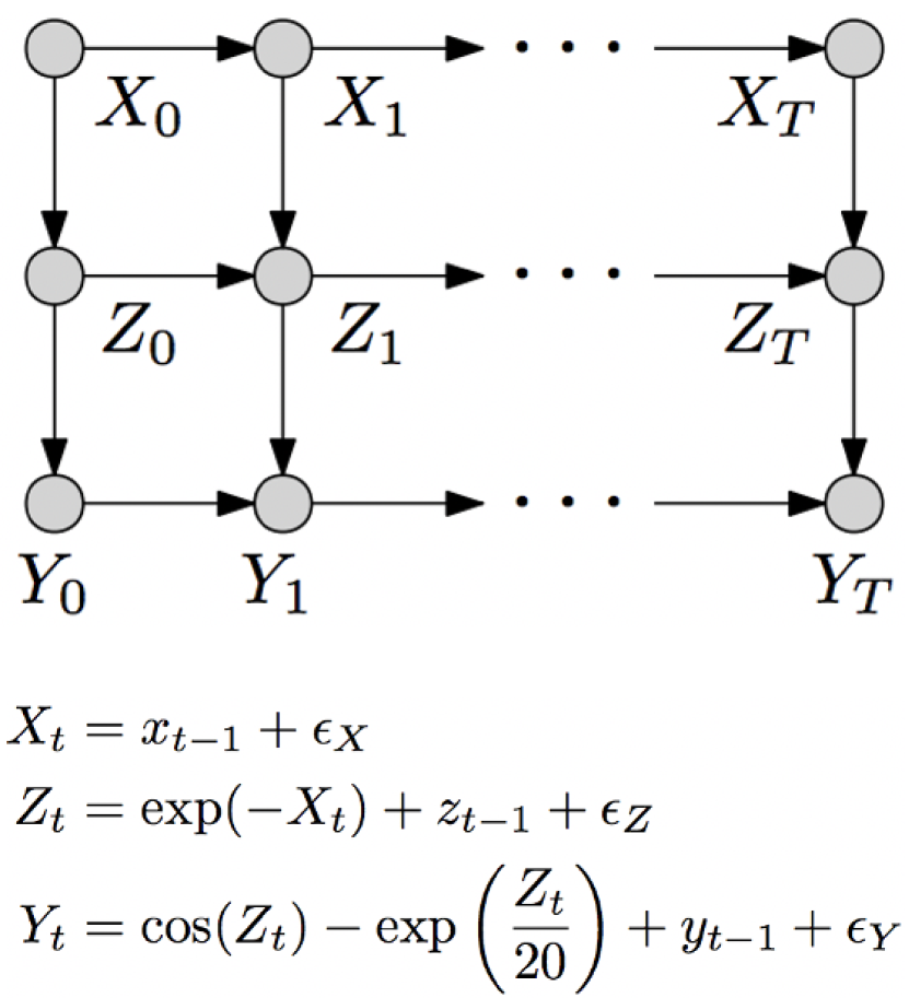
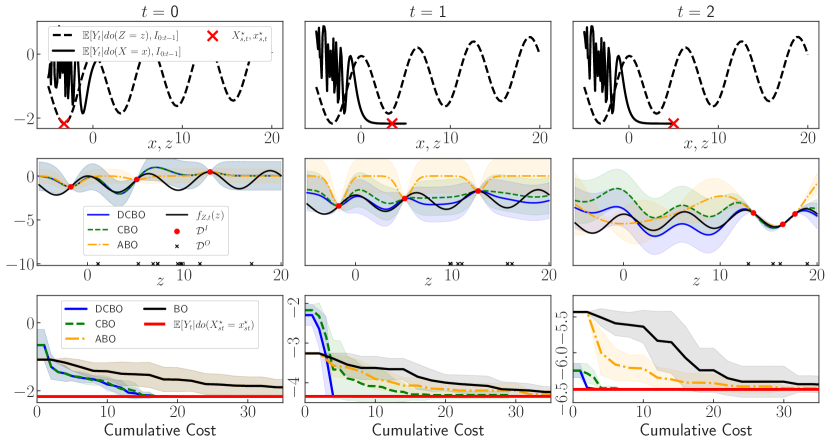
Figure 6: Stationary synthetic experiment (Stat.). Left panel: $\mathcal{G}_{0:T}$ and scm. Right panel, 1^st row: Objective functions for the sets in $\mathbb{M}=\{\{Z\},\{X\}\}$. Right panel, 2^nd row: Posterior gp obtained when using the dynamic causal gp construction vs alternative models. Right panel, 3^rd row: Convergence of dcbo and alternative models to the true optimum (red line) across 10 replicates. Shaded areas give $\pm$ one standard deviation.

E.2 Noisy manipulative variables (Noisy)

The scm used for this experiments is given by:

$$X_{t} =X_{t-1}\mathds{1}_{t>0}+\epsilon_{X}$$

$$Z_{t} =\exp(-X_{t})+Z_{t-1}\mathds{1}_{t>0}+\epsilon_{Z}$$

$$Y_{t} =\text{cos}(Z_{t})-\exp(-Z_{t}/20)+Y_{t-1}\mathds{1}_{t>0}+\epsilon_{Y}$$

where, differently from before, we have $\epsilon_{Y}\sim\mathcal{N}(0,1)$ and $\epsilon_{i}\sim\mathcal{N}(2,4)$ for $i\in\{X,Z\}$. We keep the remaining parameters equal to the previous experiment. This means $T=3$, $N=10$, $D(X_{t})=\{-5.0,5.0\}$ and $D(Z_{t})=\{-5.0,20.0\}$.

E.3 Missing observational data (Miss.)

For this experiment we use the same scm of the experiment Stat. However, we set $T=6$, $N=10$ for the first three time steps and $N=0$ afterwards. Fig. 7 shows the convergence paths for this experiment. In this setting dcbo consistently outperform cbo at every time step. However, notice how abo performance improves over time and outperforms dcbo starting from $t=5$. This is due to the ability of abo to learn the time dynamic of the objective function and exploit all interventional data collected over time to predict at the next time step.

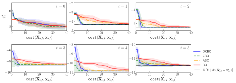
Figure 7: Experiment Miss.. Convergence of dcbo and competing methods across replicates. The red line gives the optimal $y^{*}_{t},\forall t$. Shaded areas are $\pm$ standard deviation.

E.4 Multivariate intervention sets (Multiv.)

The scm used for this experiments is given by:

$$W_{t} =\epsilon_{W}$$

$$X_{t} =-X_{t-1}\mathds{1}_{t>0}+\epsilon_{X}$$

$$Z_{t} =\text{sin}(W_{t})-Z_{t-1}\mathds{1}_{t>0}+\epsilon_{Z}$$

$$Y_{t} =-2*\exp(-(X_{t}-1)^{2})-\text{exp}(-(X_{t}+1)^{2})-(Z_{t}-1)^{2}$$

$$\;\;\;\;-Z_{T}^{2}+\text{cos}(Z_{t}*Y_{t-1})-Y_{t-1}\mathds{1}_{t>0}+\epsilon_{Y}$$

where $\epsilon_{i}\sim\mathcal{N}(0,1)$ for $i\in\{X,Z,W,Y\}$. We set $T=3$, $N=500$, $D(X_{t})=\{-5.0,5.0\}$, $D(Z_{t})=\{-5.0,20.0\}$ and $D(W_{t})=\{-3.0,3.0\}$. Notice that here dcbo and cbo explore the set $\mathbb{M}_{t}=\{\{X_{t}\},\{Z_{t}\},\{X_{t},Z_{t}\}\}$ while bo and abo intervene on $\{X_{t},Z_{t},W_{t}\}$. Fig. 8 shows the convergence paths for this experiment.

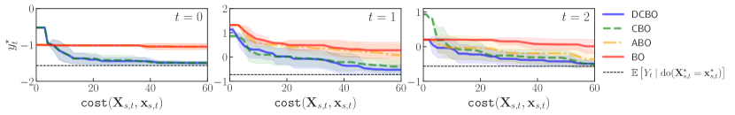
Figure 8: Experiment Multiv.. Convergence of dcbo and competing methods across replicates. The red line gives the optimal $y^{*}_{t},\forall t$. Shaded areas are $\pm$ standard deviation.

E.5 Independent manipulative variables (Ind.)

The scm used for this experiments is given by:

$$X_{t} =-X_{t-1}\mathds{1}_{t>0}+\epsilon_{X}$$

$$Z_{t} =-Z_{t-1}\mathds{1}_{t>0}+\epsilon_{Z}$$

$$Y_{t} =-2*\exp(-(X_{t}-1)^{2})-\text{exp}(-(X_{t}+1)^{2})-(Z_{t}-1)^{2}$$

$$\;\;\;\;-Z_{T}^{2}+\text{cos}(Z_{t}*Y_{t-1})-Y_{t-1}\mathds{1}_{t>0}+\epsilon_{Y}$$

where $\epsilon_{i}\sim\mathcal{N}(0,1)$ for $i\in\{X,Z,Y\}$. We set $T=3$, $N=10$, $D(X_{t})=\{-5.0,5.0\}$ and $D(Z_{t})=\{-5.0,20.0\}$. Notice that here dcbo and cbo explore the set $\mathbb{M}_{t}=\{\{X_{t}\},\{Z_{t}\},\{X_{t},Z_{t}\}\}$ while bo and abo intervene on $\{X_{t},Z_{t}\}$. In this case, exploring $\mathbb{M}_{t}$ and propagating uncertainty in the causal prior slows down dcbo convergence, see Fig. 9.

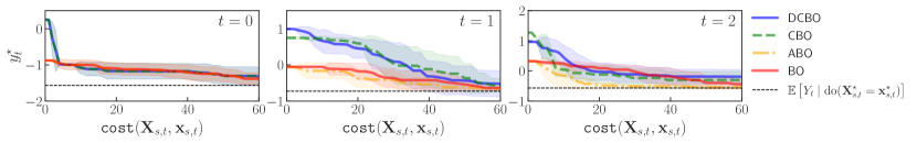
Figure 9: Experiment Ind. Convergence of dcbo and competing methods across replicates. The red line gives the optimal $y^{*}_{t},\forall t$. Shaded areas are $\pm$ standard deviation.

E.6 Non-stationary dag and scm (NonStat.)

The scm used for this experiment is more complex than the others due to the fact that the dag is non-stationary but so too is the scm:

$$\begin{cases}f(t)&\text{if }t=0\\ g(t)&\text{if }t=1\\ h(t)&\text{if }t=2\end{cases}$$ (20)

where

$$f(t)=\begin{cases}X_{t}&=\epsilon_{X}\\ Z_{t}&=X_{t}+\epsilon_{Z}\\ Y_{t}&=\sqrt{|36-(Z_{t}-1)^{2}|}+1+\epsilon_{Y}\end{cases}$$

$$g(t)=\begin{cases}X_{t}&=X_{t-1}+\epsilon_{X}\\ Z_{t}&=-\frac{X_{t}}{X_{t-1}}+Z_{t-1}+\epsilon_{Z}\\ Y_{t}&=Z_{t}\cos(Z_{t}\pi)-Y_{t-1}+\epsilon_{Y}\end{cases}$$

$$h(t)=\begin{cases}X_{t}&=X_{t-1}+\epsilon_{X}\\ Z_{t}&=X_{t}+Z_{t-1}+\epsilon_{Z}\\ Y_{t}&=Z_{t}-Y_{t-1}-Z_{t-1}+\epsilon_{Y}\end{cases}$$

where $\epsilon_{i}\sim\mathcal{N}(0,1)$ for $i\in\{X,Z,Y\}$. We set $T=3$, $N=10$, $D(X_{t})=\{-5.0,5.0\}$ and $D(Z_{t})=\{-5.0,20.0\}$. Notice that here dcbo and cbo explore the set $\mathbb{M}_{t}=\{\{X_{t}\},\{Z_{t}\},\{X_{t},Z_{t}\}\}$ while bo and abo intervene on $\{X_{t},Z_{t}\}$.

E.7 Real-World Economic data (Econ.)

We create an observational data set by extracting the following indicators from the oecd data portal (https://data.oecd.org/):

• gdp = gdp in milion of US dollars.

• cpi = annual growth of inflation measured by consumer price index cpi.

• taxrev = tax revenues measured as a percentage of gdp.

• hur = unemployment rate as measured by the numbers of unemployed people as a percentage of the labour force.

We manipulate these indicators to get the nodes in the dag of Fig.. 3(d). We define

$$U_{t} =\log(\textsc{hur}_{t})$$

$$T_{t} =\frac{\textsc{taxrev}_{t}*\textsc{gdp}_{t}-\textsc{taxrev}_{t-1}*\textsc{gdp}_{t-1}}{\textsc{taxrev}_{t-1}*\textsc{gdp}_{t-1}}$$

$$G_{t} =\frac{\textsc{gdp}_{t}-\textsc{gdp}_{t-1}}{\textsc{gdp}_{t-1}}$$

$$I_{t} =\textsc{cpi}_{t}$$

For this analysis we consider the annual data for 10 countries namely Australia, Canada, France, Germany, Italy, Japan, Korea, Mexico, Turkey, Great Britain and the United States of America for the period (2000 - 2019). We fit the following scm:

$$T_{t} =f_{T}(t)+\epsilon_{T}$$

$$I_{t} =f_{I}(t)+\epsilon_{I}$$

$$G_{t} =f_{G}(T_{t},I_{t})+\epsilon_{G}$$

$$U_{t} =f_{U}(G_{t},I_{t})+\epsilon_{U}$$

by placing gps on all functions $f_{i}(\cdot),i\in\{T,I,G,U\}$. This scm is then used to generate interventional data and compute the values of $y^{\star}_{t},t=2010,\dots,2012$.

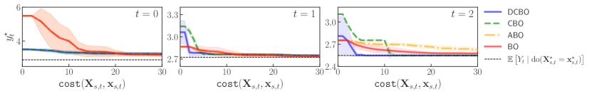
Figure 10: Experiment Econ. Convergence of dcbo and competing methods across replicates. The black line gives the optimal $y^{*}_{t},\forall t$. Shaded areas are $\pm$ one standard deviation.

We run the optimization 10 times and plot the convergence path for dcbo and competing models (see Fig. 10). While all method perform similarly at $t=2010$ and $t=2011$, dcbo outperforms competing approaches at $t=2012$. On average (see Table 1) dcbo finds the optimal intervention faster.

E.8 Results without convergence

We repeat all experiments in the paper allowing the algorithms to perform a lower number of trials at every time steps. This means that, for $t>0$, when moving to step $t$ the convergence of the algorithm at step $t-1$ is not guaranteed. In turn this affect the optimum value that the algorithm can reach at subsequent steps. Results are given in Table 3 and Table 4. The convergence paths for dcbo and competing methods are given in Fig. 11 to Fig. 15.

Table 3: Average modified gap measure (10 replicates) across time steps and for different experiments. See Fig. 1 for a summary of the compared methods. Higher values are better. The best result for each experiment is bolded. Standard errors in brackets.

	Synthetic data						Real data
	Stat.	Miss.	Noisy	Multiv.	Ind.	NonStat.	Econ.	ode
dcbo	0.88	0.72	0.73	0.49	0.47	0.47	0.40	0.67
	(0.00)	(0.07)	(0.00)	(0.00)	(0.05)	(0.00)	(0.04)	(0.00)
cbo	0.57	0.51	0.67	0.47	0.48	0.47	0.41	0.65
	(0.02)	(0.09)	(0.01)	(0.04)	(0.04)	(0.00)	(0.04)	(0.00)
abo	0.43	0.45	0.42	0.40	0.50	0.41	0.38	0.47
	(0.06)	(0.04)	(0.06)	(0.05)	(0.00)	(0.03)	(0.04)	(0.01)
bo	0.42	0.41	0.41	0.38	0.50	0.40	0.40	0.46
	(0.06)	(0.05)	(0.07)	(0.07)	(0.01)	(0.04)	(0.04)	(0.03)

Table 4: Average percentage of replicates across time steps and for different experiments for which the optimal intervention set is identified. See Fig. 1 for a summary of the compared methods. Higher values are better. The best result for each experiment is bolded.

	Synthetic data						Real data
	Stat.	Miss.	Noisy	Multiv.	Ind.	NonStat.	Econ.	ode
dcbo	90.0	70.00	93.00	93.33	96.67	66.67	73.33	33.33
cbo	76.67	63.33	76.67	86.67	93.33	33.33	80.00	33.33
abo	0.00	0.00	0.00	0.00	100.00	0.00	66.67	0.00
bo	0.00	0.00	0.00	0.00	100.00	0.00	66.67	0.00

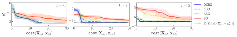
Figure 11: Experiment Stat. with maximum number of trials $H=30$. Convergence of dcbo and competing methods across replicates. The black line gives the optimal $y^{*}_{t},\forall t$. Shaded areas are $\pm$ one standard deviation.

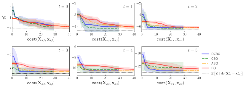
Figure 12: Experiment Miss. with maximum number of trials $H=30$. Convergence of dcbo and competing methods across replicates. The black line gives the optimal $y^{*}_{t},\forall t$. Shaded areas are $\pm$ one standard deviation.

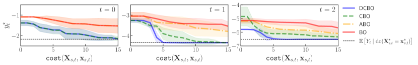
Figure 13: Experiment Noisy. with maximum number of trials $H=30$. Convergence of dcbo and competing methods across replicates. The black line gives the optimal $y^{*}_{t},\forall t$. Shaded areas are $\pm$ one standard deviation.

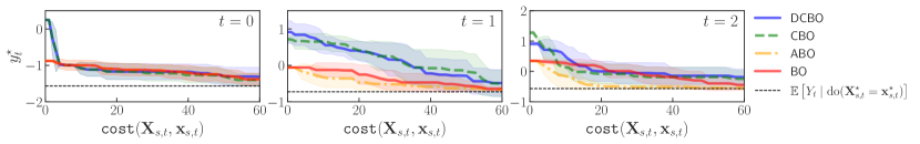
Figure 14: Experiment Ind. with maximum number of trials $H=30$. Convergence of dcbo and competing methods across replicates. The black line gives the optimal $y^{*}_{t},\forall t$. Shaded areas are $\pm$ one standard deviation.

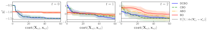
Figure 15: Experiment Multiv. with maximum number of trials $H=30$. Convergence of dcbo and competing methods across replicates. The black line gives the optimal $y^{*}_{t},\forall t$. Shaded areas are $\pm$ one standard deviation.

E.9 Results over multiple datasets and replicates

In this section we show the results obtained running all the experiments in the main paper across 10 different observational dataset sampled from the scm given above. Results are given in Table 5.

Table 5: Average modified gap measure across 10 observational datasets and 10 replicates. Results are average figures across time steps. See Fig. 1 for a summary of the compared methods. Higher values are better. The best result for each experiment is bolded. Standard errors in brackets.

	Synthetic data
	Stat.	Miss.	Noisy	Multiv.	Ind.	NonStat.
dcbo	0.83	0.82	0.82	0.48	0.46	0.63
	(0.06)	(0.05)	(0.05)	(0.02)	(0.03)	(0.06)
cbo	0.80	0.68	0.74	0.48	0.47	0.64
	(0.05)	(0.04)	(0.09)	(0.01)	(0.02)	(0.04)
abo	0.47	0.49	0.47	0.45	0.48	0.38
	(0.01)	(0.00)	(0.01)	(0.08)	(0.00)	(0.01)
bo	0.47	0.47	0.47	0.40	0.50	0.38
	(0.01)	(0.01)	(0.01)	(0.07)	(0.00)	(0.01)

Supplementary material for
Dynamic Causal Bayesian Optimisation F Intervening on differential equations (ode)

In this section we describe in detail the experiment conducted in Section 4.2. This example is based on the work by Blasius et al. [8]. In this demonstration we continue along that paradigm when we investigate a biological systems in which two species interact, one as a predator and the other as prey. Blasius et al. [8] performed microcosm experiments (in a chemostat or bioreactor) with a planktonic predator–prey system.

We use the provided ODE (Section F.2) from the paper [8, Methods], which describes a stage-structured predator–prey community in a chemostat, as our scm. As $\mathcal{D}^{O}$ we use the experimental data collected in vitro (for raw data see supplementary material of [8]). The corresponding dag (Section F.3) and scm (Section F.4) is constructed from the ODE (see overleaf), by rolling out the temporal variable dependencies in the ODE (the idea is well illustrated in [55, Fig. 1]).

Using this setup we investigate a requisite intervention policy necessary to reduce the concentration of dead animals in the chemostat – $D_{t}$ in Fig. 3(e).

F.1 Interpreting differential equations as causal models

A lot of work [47, 31, 41, 10, 27, 55] has been dedicated to interpreting ordinary differential equations as structural causal models and consequently the associated task of intervening therein. More precisely, attention has been placed on extending causal theory [45, 52] to the cyclic case, thereby enabling causal modelling of systems that involve feedback [41, 33, 17, 42, 30, 49, 47].

Naively, the simplest extension to the cyclical case is by simply dropping the acyclicity constraint from the scm [41, §1]. But then we are faced with a new problem: how do we “interpret cyclic structural equations” [41]? The most common approach is to “assume an underlying discrete-time dynamical system, in which the structural equations are used as fixed point equations” [41]. This renders a simple schema wherein which we use the scm as a set of updates rules, to find the values of the variables at $t+1$, using the information from $t$. This is a popular paradigm, advanced by e.g. Spirtes [52], Hyttinen et al. [30], Dash [15], Lacerda et al. [34], Mooij et al. [40]. This is also the one we will use herein.

Another philosophy that deals with interventions in systems, was developed by Casini et al. [12]. In the same vein is the work by Gebharter [22], Gebharter & Schurz [23]. This suite of work comes from the philosophy of science domain, rather than the statistical and machine learning literature, briefly reviewed in the previous two paragraphs. Theirs is primarily a concern with mechanisms (specifically “mechanistic biological models with complex dynamics” in the case of Kaiser [31]) – fundamentally they are the same thing as our causal effects but the perspective is different. Casini et al. [12] suggests that modelling (acyclical) mechanisms should be done by way of recursive Bayesian networks (RBN). Gebharter [22] points out some shortcomings with Caisini’s approach and proposes the multilevel causal model (MLCM) as a remedy. Notably though, both works assume acyclicity (and so cannot feature mechanisms with feedback) of the problem domain a shortcoming that Gebharter & Schurz [23] deals with by extending the MLCM to allow for cycles. For completeness we should also say that the RBN was extended to handle cycles by Clarke et al. [13] (their approach was used Gebharter & Schurz [23] for extending the MLCM).

F.2 Ordinary differential equation

Blasius et al. [8] develop a mathematical model, the set of ordinary differential equations in Eq. 21–Eq. 26, to describe a stage-structured predator–prey community in a chemostat, which closely follows their experimental setup.

$$\frac{\text{d}N}{\text{d}t} =\delta N_{\textrm{in}}-F_{P}(N)P-\delta N$$ (21)

$$\frac{\text{d}P}{\text{d}t} =F_{P}(N)P-\frac{F_{B}(P)B}{\varepsilon}-\delta P$$ (22)

$$\frac{\text{d}E}{\text{d}t} =R_{E}-R_{J}-\delta E$$ (23)

$$\frac{\text{d}J}{\text{d}t} =R_{J}-R_{A}-(m+\delta)J$$ (24)

$$\frac{\text{d}A}{\text{d}t} =\beta R_{A}-(m+\delta)A$$ (25)

$$\frac{\text{d}D}{\text{d}t} =m(J+A)-\delta D$$ (26)

A full description of all variables and parameters can be found in Table 6.

Table 6: Table describing variable and parameters of ODE in Eq. 21 – Eq. 26.

Variable	Description	Value	Unit
$N$	Nitrogen (prey) concentration	$\in\mathbb{R}^{1}$	$\mu\text{mol}\cdot\text{N}\cdot\text{L}^{-1}$
$P$	Phytoplankton (predator) concentration	$\in\mathbb{R}^{1}$	$\mu\text{mol}\cdot\text{N}\cdot\text{L}^{-1}$
$E$	Predator egg concentration	$\in\mathbb{R}^{1}$	$\mu\text{mol}\cdot\text{N}\cdot\text{L}^{-1}$
$J$	Predator juvenile concentration	$\in\mathbb{R}^{1}$	$\mu\text{mol}\cdot\text{N}\cdot\text{L}^{-1}$
$A$	Predator adult concentration	$\in\mathbb{R}^{1}$	$\mu\text{mol}\cdot\text{N}\cdot\text{L}^{-1}$
$D$	Dead animal concentration	$\in\mathbb{R}^{1}$	$\mu\text{mol}\cdot\text{N}\cdot\text{L}^{-1}$
Parameter	Description	Value	Unit
$N_{\text{in}}$	Nitrogen concentration in the external medium	80	$\mu\text{mol}\cdot\text{N}\cdot\text{L}^{-1}$
$F_{P}$	Algal nutrient uptake	-	$\mu\text{mol}\cdot\text{N}\cdot\text{L}^{-1}$
$F_{B}$	Rotifer nutrient uptake	-	$\mu\text{mol}\cdot\text{N}\cdot\text{L}^{-1}$
$\varepsilon$	Predator assimilation efficiency	0.55	-
$R_{E}$	Egg recruitment rate	-	-
$R_{J}$	Juvenile recruitment rate	-	-
$R_{A}$	Adult recruitment rate	-	-
$m$	Rotifer (predator) mortality rate	0.15	Per day
$\beta$	Adult/juvenile mass ratio	5	-

For additional details see [8, Methods].

F.3 Corresponding directed acyclical graph

The original rolled-out dag (Fig. 16(b)) is modified to remove graph cycles (Fig. 16(c)), where the corresponding dependencies are replicated in the scm. Now, note first that the temporal roll-out of Fig. 16(a) contains no cycles (once the self-cycles have been re-purposed as temporal transition functions). Nonetheless, comparing Fig. 16(b) and Fig. 16(c) it can be seen that two edges have been removed to simplify the causal dependencies on the phytoplankton (predator) concentration i.e. to make it only dependent on the nitrogen concentration in the external medium as well as the most immediate predator concentration at time $t-1$.

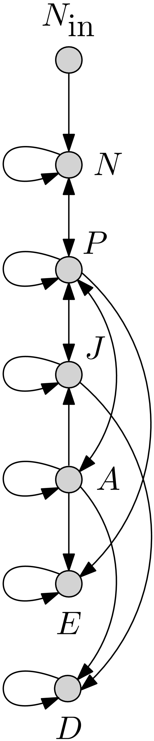
(a) ODE variable dependencies.

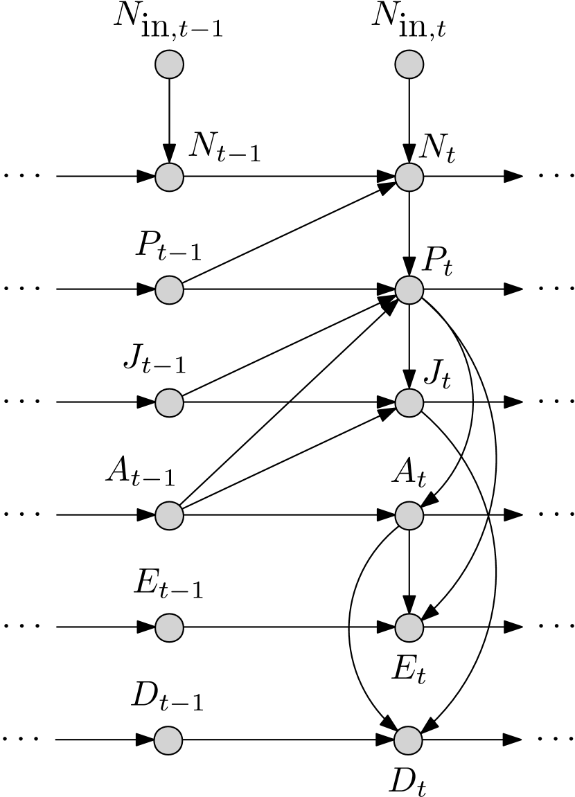
(b) First DAG approximation.

(c) Second DAG approximation.

Figure 16: Proposed time-indexed DAG representing the causal dependencies in the stage-structured predator–prey community in a chemostat. The vertices of the graph represent the concentrations of the different chemostat compounds at different discrete time points, where time is moving from left to right. Fig. 16(a) shows the variable dependencies as described in the original ODE found in Eq. 21 – Eq. 26 – notice the presence of self-loops and cycles. Figure 16(b) shows a first approximation to a corresponding causal graph, where the ODE has been ‘rolled’ out in time – note the absence of self-loops and cycles. Figure 16(c) shows a second approximation to the original ODE dynamics but this time removing two parent dependencies from $P_{t}$.

One large deviation from the original set of ODEs, is that we treat the $N_{\text{in}}$ as an instrument variable and moreover allow it to be manipulative. This means that in order to reduce the concentration $D_{t}$ we allow the optimisation frameworks to intervene also on $N_{\text{in}}$.

F.4 ODE as SEM

We fit the following scm, based on the dag in Fig. 16(c):

$$N_{\text{in},t} =\epsilon_{N_{\text{in}}}$$ (27)

$$N_{t} =f_{N}(N_{\textrm{in},t},N_{t-1},P_{t-1})+\epsilon_{N}$$ (28)

$$P_{t} =f_{P}(N_{t},P_{t-1})+\epsilon_{P}$$ (29)

$$J_{t} =f_{J}(P_{t},J_{t-1},A_{t-1})+\epsilon_{J}$$ (30)

$$A_{t} =f_{A}(P_{t},A_{t-1})+\epsilon_{A}$$ (31)

$$E_{t} =f_{E}(P_{t},A_{t},E_{t-1})+\epsilon_{E}$$ (32)

$$D_{t} =f_{D}(J_{t},A_{t},D_{t-1})+\epsilon_{D}$$ (33)

by placing gps on all functions $\{f_{i}(\cdot)\mid i\in\{N_{\text{in}},N,P,E,J,A,D\}\}$. This scm is then used to generate interventional data and compute the values of $\{d^{\star}_{t}\mid t=0,1,2\}$.

Further, $\{\epsilon_{j}\sim\mathcal{N}(0,1)\mid j\in\{N_{\text{in}},N,P,E,J,A,D\}\}$. We set $T=3$, $N=4$ where the manipulative variables are: $N_{\text{in},t},J_{t}$ and $A_{t}$. This means in practise that we are interested in the start of the simulation where we are trying to reduce the mortality concentration, in the chemostat, from beginning where our observational samples $\mathcal{D}^{O}$ are formed from four time-series.

Intervention domains are given by

$$D(N_{\text{in},t}) =[40.0,160.0]$$

$$D(J_{t}) =[0.0,20.0]$$

$$D(A_{t}) =[0.0,100.0]$$

Notice that dcbo and cbo explore the set

$$\mathbb{M}_{t}=\{\{N_{\text{in},t}\},\{J_{t}\},\{A_{t}\},\{N_{\text{in},t},J_{t}\},\{N_{\text{in},t},A_{t}\},\{J_{t},A_{t}\},\{N_{\text{in},t},J_{t},A_{t}\}\}$$

while bo and abo will only intervene on $\{N_{\text{in},t},J_{t},A_{t}\}$. The optimal sequence of interventions is given by $\{\{J_{0},A_{0}\},\{M_{1}\},\{M_{2}\}\}$.

Results are shown in Fig. 17. Note that the performance of dcbo and cbo are almost identical.

Figure 17: Experiment ode with maximum number of trials $H=20$. Convergence of dcbo and competing methods across replicates. The black line gives the optimal $y^{*}_{t},\forall t$. Shaded areas are $\pm$ one standard deviation.

Supplementary material for
Dynamic Causal Bayesian Optimisation G Applicability of dcbo to real-world problems

As previously done in cbo [4] and other causal decision-making frameworks (e.g. [6]) for static settings, in dcbo we assume to be able to repeatedly intervene in the system with interventions that have an instantaneous effect observed within the time slice duration. In other words, within every time step, we perform an intervention that changes the system and that leads to an effect for which we collect the corresponding target experimental value. However, the system reverts back once the experiment has been implemented and the agent can then explore alternative interventions and measure their effect too. In dcbo, the dynamics of the time resolution specified by the graph time indices is slower than the time you can take actions and see the effects.

While this assumption can be difficult to verify when interacting directly with the psychical world, it does not limit the applicability of the proposed framework to real-world problems. Indeed, in a variety of real-world settings, simulators or digital twins of real-world assets/processes are used in industrial settings and are fundamental in selecting actions before intervening in the real physical world. Digital twins provide virtual replicas of a physical object or system, such as a bridge or an engine, that engineers use for simulations before something is created or to monitor its operation in real-time. Examples are given by the digital twin of a 3D-printed stainless steel bridge [bridge], nasa and u.s. Air Force vehicles [24], jet-engine monitoring, infrastructure inspection as well as cardiac medicine [2]. In all these settings, observational data are used to build the emulator which is “a living computer model which is continuously learning to imitate the physical world” [bridge]. We can then intervene on the digital twin to collect interventional data and measure the causal effects. Intervening in a simulator has a cost e.g. a computationally cost thus interventions need to be carefully picked by employing a probabilistic model that correctly quantifies uncertainty and integrates different sources of information. In dcbo this is done by using the dynamic causal gp model. Once an intervention has been implemented, the digital twin “reverts” to its unperturbed/observational nature (i.e. without intervention), allowing the user to investigate other interventions without having changed the “underlying state of the system” nor, indeed, the true system. Once an optimal intervention is found, the agent can implement it in the real system thus changing it. Note that our approach allows for noise in the likelihood function thus the simulator can be a noisy version of the physical world.

Supplementary material for
Dynamic Causal Bayesian Optimisation H Connections

We conclude by providing a discussion of the links between dcbo, the two methodologies used as benchmarks in the experimental session, namely the cbo algorithm [4] and the abo algorithm [43], and the literature on bandits and rl. We discuss how their problem setups differ from our and highlight the reasons why dcbo is needed to solve the problem in Eq. (1).

cbo algoritm

The cbo algorithm [4] can be used to find optimal interventions to perform in a causal graph so as to optimize a single target node $Y$. cbo addresses static settings where variables in $\mathcal{G}$ are i.i.d. across time steps, i.e. $p(\mathbf{V}_{t})=p(\mathbf{V})\text{,}\forall t$, and only one static target variable exists. For instance, cbo can be used to find the optimal intervention for $Y$ in the dag of Fig. 1b. In order to use cbo for the dag of Fig. 1a, one would need to identify a unique target among $Y_{0:T}$, e.g. $Y_{T}$. However, optimizing $Y_{T}$ might lead to chose interventions that are sub-optimal for $Y_{0:T-1}$ thus not solving the problem in Eq. (1). In addition, to find the optimal intervention for $Y_{T}$, cbo explores all interventions in $\mathcal{P}(\mathbf{X}_{0:T})$ which results in a large search space and requires performing a high number of interventions. This slows down the convergence of the algorithm and increases the optimization cost. One can alternatively run cbo $T$ times optimizing $Y_{t}$ at each time step. Doing that would require re-initializing the surrogate models for the objective functions at every $t$ and would thus imply loosing all the information collected from previous interventions. Finally, in optimizing $Y_{t}$, cbo does not account for how the previously taken interventions have changed the system again slowing down the convergence of the algorithm. In order to recursively optimise intermediate outputs given the previously taken decisions one need to resort to dcbo. By changing the objective function at every time step, incorporating prior interventional information in the objective function and limiting the search space at every time step based on the topology of the $\mathcal{G}$, dcbo addresses the cbo issues mentioned above making it a framework that can be practically used for sequential decision making in a variety of applications.

abo algorithm

While cbo tackles the causal dimension of the dcgo problem but not the temporal dimension, the abo algorithm also addresses dynamic settings but does not account for the causal relationships among variables, see Fig. 1 for a graphical representation of the relationship between these methods. As in bo, abo finds the optimal intervention values by breaking the causal dependencies between the inputs and intervening simultaneously on all of them thus setting $\mathbf{X}_{s,t}=\mathbf{X}_{t}$ for all $t$. Additionally, considering the inputs as fixed and not as random variables, abo does not account for their temporal evolution. This is reflected in the dag of Fig. 1(c) where both the horizontal links between the inputs and the edges amongst the input variables are missing. In solving the problem in Eq. (1) for the dag in Fig. 1a, bo would disregard both the temporal dependencies in $Y$ and the input dependencies (dag in Fig. 1d) while abo would keep the former but ignore the latter. Differently from our approach, abo considers a continuous time space and places a surrogate model on $Y_{t}=f(\mathbf{x},t)$. $f(\mathbf{x},t)$ is then modelled via a spatio-temporal gp with separable kernel. The abo acquisition function for $f(\mathbf{x},t)$ is then restricted to avoid collecting points in the past or too far ahead in the future where the gp predictions have high uncertainty. The spatio-temporal gp allows abo to predict the objective function ahead in time and track the evolution of the optimum. However, in order for abo to work the objective function rate of change over time must be slow enough to gather enough samples to learn the relationships in space and time. In our discrete time setting this condition is equivalent to ask that, at every time step, it is possible to perform different interventions with an underlying true function that does not change. Note that also in dcbo, Assumptions 1 imply a certain level of regularity in the objective functions. For instance, in the dag of Fig. 1a, given that $\text{Pa}\!\left(Y_{t}\right)=\{Z_{t},Y_{t-1}\},\forall t>0$, the objective functions have a constant shape and are only shifted vertically by the performed interventions. While some regularity is also required in dcbo, through the causal graph we impose more structure on the objective function and its input thus lowering the need for exploration. The more accurate the estimation of the functions in the scm is the more we can track the dynamic of the objective function and we can deal with sharp changes in the objectives. One additional important difference between abo and dcbo is in the exploration of different intervention set. Indeed, by intervening on all variables, abo can lead to sub-optimal solution. As mentioned for bo in [4], depending on the structural relationships between variables, intervening on a subgroup might lead to a propagation of effects in the causal graph and a higher final target. In addition, intervening on all variables is cost-ineffective in cases when the same target can be obtained by setting only a subgroup of them. This is particularly true in the time setting as the optimal intervention set might not only be a subset of $\mathcal{P}(\mathbf{X}_{t})$ but might also evolve overtime.

Bandits and rl In the broader decision-making literature, causal relationships have been previously considered in the context of multi-armed bandit problems [mab, 6, 35, 36, 37] and reinforcement learning [rl, 38, 11, 20, 58, 39]. In these cases, the actions or arms correspond to interventions on an arbitrary causal graph where there exists complex links between the agent’s decisions and the received rewards. Causal mab algorithms focus on static settings where the distribution of the rewards is stationary and is not affected by the pulled arms. In addition, mab focus on intervention on discrete variable and only deal with the problem of selecting the right intervention set but not the intervention value. Differently from dcbo, rl algorithms explicitly model the state dynamic and account for the way each action affect the state of the environment. dcbo setting differs from both causal rl and causal mab. dcbo does not have a notion of state and therefore does not require an explicit model of its dynamic. The system is fully specified by the causal graph and the connected structural equation model. As in bo, dcbo does not aim at learning an optimal policy but rather a set of optimal actions. Furthermore, within each time step, dcbo allows the agent to perform a number of explorative interventions which are not modifying the environment. Once the optimal action is identified this is propagated in the system thus changing it. Differently from both mab and rl, dcbo is myopic that is interventions are decided by maximizing the one-step ahead utility function. We leave the integration of dcbo with a non-myopic bo scheme to future work.

References

• [1] Digital twin of the world’s first 3d printed stainless steel bridge. https://www.turing.ac.uk/research/research-projects/digital-twin-worlds-first-3d-printed-stainless-steel-bridge. Accessed: August 7th, 2021.
• [2] Creating a virtual replica. https://www.ingenia.org.uk/getattachment/dc398efc-4995-46b8-ad8b-8414a413b27a/Digital-twins.pdf. Accessed: August 7th, 2021.
• Aglietti et al. [2020a] Aglietti, V., Damoulas, T., Álvarez, M., and González, J. Multi-task Causal Learning with Gaussian Processes. In Advances in Neural Information Processing Systems 33 pre-proceedings (NeurIPS), 2020a.
• Aglietti et al. [2020b] Aglietti, V., Lu, X., Paleyes, A., and González, J. Causal Bayesian Optimization. In Proceedings of the Twenty Third International Conference on Artificial Intelligence and Statistics, volume 108 of Proceedings of Machine Learning Research, pp.  3155–3164. PMLR, 26–28 Aug 2020b.
• Azimi et al. [2011] Azimi, J., Jalali, A., and Fern, X. Dynamic batch bayesian optimization. arXiv preprint arXiv:1110.3347, 2011.
• Bareinboim et al. [2015] Bareinboim, E., Forney, A., and Pearl, J. Bandits with unobserved confounders: A causal approach. Advances in Neural Information Processing Systems, 28:1342–1350, 2015.
• Besbes et al. [2014] Besbes, O., Gur, Y., and Zeevi, A. Stochastic multi-armed-bandit problem with non-stationary rewards. Advances in neural information processing systems, 27:199–207, 2014.
• Blasius et al. [2020] Blasius, B., Rudolf, L., Weithoff, G., Gaedke, U., and Fussmann, G. F. Long-term cyclic persistence in an experimental predator–prey system. Nature, 577(7789):226–230, 2020.
• Bogunovic et al. [2016] Bogunovic, I., Scarlett, J., and Cevher, V. Time-varying gaussian process bandit optimization. In Artificial Intelligence and Statistics, pp.  314–323. PMLR, 2016.
• Bongers & Mooij [2018] Bongers, S. and Mooij, J. M. From random differential equations to structural causal models: The stochastic case. arXiv preprint arXiv:1803.08784, 2018.
• Buesing et al. [2018] Buesing, L., Weber, T., Zwols, Y., Racaniere, S., Guez, A., Lespiau, J.-B., and Heess, N. Woulda, coulda, shoulda: Counterfactually-guided policy search. arXiv preprint arXiv:1811.06272, 2018.
• Casini et al. [2011] Casini, L., Illari, P. M., Russo, F., and Williamson, J. Models for prediction, explanation and control: recursive bayesian networks. THEORIA. Revista de Teoría, Historia y Fundamentos de la Ciencia, 26(1):5–33, 2011.
• Clarke et al. [2014] Clarke, B., Leuridan, B., and Williamson, J. Modelling mechanisms with causal cycles. Synthese, 191(8):1651–1681, 2014.
• Cruz et al. [2011] Cruz, C., González, J. R., and Pelta, D. A. Optimization in dynamic environments: a survey on problems, methods and measures. Soft Computing, 15(7):1427–1448, 2011.
• Dash [2005] Dash, D. Restructuring dynamic causal systems in equilibrium. In AISTATS. Citeseer, 2005.
• De et al. [2006] De, M. K., Slawomir, N. J., and Mark, B. Stochastic diffusion search: Partial function evaluation in swarm intelligence dynamic optimisation. In Stigmergic optimization, pp.  185–207. Springer, 2006.
• Dechter [1996] Dechter, R. Identifying independencies in causal graphs with feedback. In Uncertainty in Artificial Intelligence: Proceedings of the… Conference on Uncertainty in Artificial Intelligence, pp.  420. Morgan Kaufmann Pub., 1996.
• Duvenaud [2014] Duvenaud, D. Automatic model construction with Gaussian processes. PhD thesis, University of Cambridge, 2014.
• Duvenaud et al. [2011] Duvenaud, D., Nickisch, H., and Rasmussen, C. E. Additive Gaussian Processes. arXiv preprint arXiv:1112.4394, 2011.
• Foerster et al. [2018] Foerster, J., Farquhar, G., Afouras, T., Nardelli, N., and Whiteson, S. Counterfactual multi-agent policy gradients. In Proceedings of the AAAI Conference on Artificial Intelligence, volume 32, 2018.
• Fogel et al. [1966] Fogel, L. J., Owens, A. J., and Walsh, M. J. Artificial intelligence through simulated evolution. 1966.
• Gebharter [2014] Gebharter, A. A formal framework for representing mechanisms? Philosophy of Science, 81(1):138–153, 2014.
• Gebharter & Schurz [2016] Gebharter, A. and Schurz, G. A modeling approach for mechanisms featuring causal cycles. Philosophy of Science, 83(5):934–945, 2016.
• Glaessgen & Stargel [2012] Glaessgen, E. and Stargel, D. The digital twin paradigm for future nasa and us air force vehicles. In 53rd AIAA/ASME/ASCE/AHS/ASC structures, structural dynamics and materials conference 20th AIAA/ASME/AHS adaptive structures conference 14th AIAA, pp.  1818, 2012.
• Glymour et al. [2019] Glymour, C., Zhang, K., and Spirtes, P. Review of causal discovery methods based on graphical models. Frontiers in Genetics, 10, 2019.
• Goldberg & Smith [1987] Goldberg, D. E. and Smith, R. E. Nonstationary function optimization using genetic algorithms with dominance and diploidy. In Genetic algorithms and their applications: proceedings of the second International Conference on Genetic Algorithms: July 28-31, 1987 at the Massachusetts Institute of Technology, Cambridge, MA. Hillsdale, NJ: L. Erlhaum Associates, 1987., 1987.
• Hansen et al. [2014] Hansen, N., Sokol, A., et al. Causal interpretation of stochastic differential equations. Electronic Journal of Probability, 19, 2014.
• Huang et al. [2019] Huang, B., Zhang, K., Gong, M., and Glymour, C. Causal discovery and forecasting in nonstationary environments with state-space models. In International Conference on Machine Learning, pp. 2901–2910. PMLR, 2019.
• Huang et al. [2006] Huang, D., Allen, T. T., Notz, W. I., and Zeng, N. Global optimization of stochastic black-box systems via sequential kriging meta-models. Journal of global optimization, 34(3):441–466, 2006.
• Hyttinen et al. [2012] Hyttinen, A., Eberhardt, F., and Hoyer, P. O. Learning linear cyclic causal models with latent variables. The Journal of Machine Learning Research, 13(1):3387–3439, 2012.
• Kaiser [2016] Kaiser, M. I. On the limits of causal modeling: spatially-structurally complex biological phenomena. Philosophy of Science, 83(5):921–933, 2016.
• Koller & Friedman [2009] Koller, D. and Friedman, N. Probabilistic Graphical Models: Principles and Techniques - Adaptive Computation and Machine Learning. The MIT Press, 2009. ISBN 0262013193.
• Koster et al. [1996] Koster, J. T. et al. Markov properties of nonrecursive causal models. Annals of statistics, 24(5):2148–2177, 1996.
• Lacerda et al. [2012] Lacerda, G., Spirtes, P. L., Ramsey, J., and Hoyer, P. O. Discovering cyclic causal models by independent components analysis. arXiv preprint arXiv:1206.3273, 2012.
• Lattimore et al. [2016] Lattimore, F., Lattimore, T., and Reid, M. D. Causal bandits: Learning good interventions via causal inference. In Advances in Neural Information Processing Systems, pp. 1181–1189, 2016.
• Lee & Bareinboim [2018] Lee, S. and Bareinboim, E. Structural causal bandits: where to intervene? Advances in Neural Information Processing Systems 31, 31, 2018.
• Lee & Bareinboim [2019] Lee, S. and Bareinboim, E. Structural causal bandits with non-manipulable variables. In Proceedings of the AAAI Conference on Artificial Intelligence, volume 33, pp.  4164–4172, 2019.
• Lu et al. [2018] Lu, C., Schölkopf, B., and Hernández-Lobato, J. M. Deconfounding reinforcement learning in observational settings. arXiv preprint arXiv:1812.10576, 2018.
• Madumal et al. [2020] Madumal, P., Miller, T., Sonenberg, L., and Vetere, F. Explainable reinforcement learning through a causal lens. In Proceedings of the AAAI Conference on Artificial Intelligence, volume 34, pp.  2493–2500, 2020.
• Mooij et al. [2011] Mooij, J. M., Janzing, D., Heskes, T., and Schölkopf, B. On causal discovery with cyclic additive noise model. In Advances in Neural Information Processing Systems 33 pre-proceedings (NeurIPS), 2011.
• Mooij et al. [2013] Mooij, J. M., Janzing, D., and Schölkopf, B. From ordinary differential equations to structural causal models: The deterministic case. In Proceedings of the Twenty-Ninth Conference on Uncertainty in Artificial Intelligence, UAI’13, pp.  440–448, Arlington, Virginia, USA, 2013. AUAI Press.
• Neal [2000] Neal, R. M. On deducing conditional independence from d-separation in causal graphs with feedback (research note). Journal of Artificial Intelligence Research, 12:87–91, Mar 2000. ISSN 1076-9757. doi: 10.1613/jair.689. URL http://dx.doi.org/10.1613/jair.689.
• Nyikosa et al. [2018] Nyikosa, F. M., Osborne, M. A., and Roberts, S. J. Bayesian optimization for dynamic problems, 2018.
• Pearl [1995] Pearl, J. Causal diagrams for empirical research. Biometrika, 82(4):669–688, 1995.
• Pearl [2000] Pearl, J. Causality: models, reasoning and inference, volume 29. Springer, 2000.
• Pelta et al. [2009] Pelta, D., Cruz, C., and Verdegay, J. L. Simple control rules in a cooperative system for dynamic optimisation problems. International Journal of General Systems, 38(7):701–717, 2009.
• Peters et al. [2020] Peters, J., Bauer, S., and Pfister, N. Causal models for dynamical systems. arXiv preprint arXiv:2001.06208, 2020.
• Rasmussen [2003] Rasmussen, C. E. Gaussian processes in machine learning. In Summer School on Machine Learning, pp.  63–71. Springer, 2003.
• Rubenstein et al. [2016] Rubenstein, P. K., Bongers, S., Schölkopf, B., and Mooij, J. M. From deterministic odes to dynamic structural causal models. arXiv preprint arXiv:1608.08028, 2016.
• Shahriari et al. [2015] Shahriari, B., Swersky, K., Wang, Z., Adams, R. P., and De Freitas, N. Taking the human out of the loop: A review of bayesian optimization. Proceedings of the IEEE, 104(1):148–175, 2015.
• Silva & Gramacy [2010] Silva, R. and Gramacy, R. B. Gaussian Process Structural Equation Models with Latent Variables. arXiv preprint arXiv:1002.4802, 2010.
• Spirtes [1995] Spirtes, P. Directed cyclic graphical representations of feedback models. In Proceedings of the Eleventh Conference on Uncertainty in Artificial Intelligence, UAI’95, pp.  491–498, San Francisco, CA, USA, 1995. Morgan Kaufmann Publishers Inc. ISBN 1558603859.
• Trojanowski & Wierzchoń [2009] Trojanowski, K. and Wierzchoń, S. T. Immune-based algorithms for dynamic optimization. Information Sciences, 179(10):1495–1515, 2009.
• Villar et al. [2015] Villar, S. S., Bowden, J., and Wason, J. Multi-armed bandit models for the optimal design of clinical trials: benefits and challenges. Statistical science: a review journal of the Institute of Mathematical Statistics, 30(2):199, 2015.
• Weber [2016] Weber, M. On the incompatibility of dynamical biological mechanisms and causal graphs. Philosophy of Science, 83(5):959–971, 2016.
• Witty et al. [2020] Witty, S., Takatsu, K., Jensen, D., and Mansinghka, V. Causal Inference using Gaussian Processes with Structured Latent Confounders. In International Conference on Machine Learning, pp. 10313–10323. PMLR, 2020.
• Wu et al. [2018] Wu, Q., Iyer, N., and Wang, H. Learning contextual bandits in a non-stationary environment. In The 41st International ACM SIGIR Conference on Research & Development in Information Retrieval, pp.  495–504, 2018.
• Zhang & Bareinboim [2019] Zhang, J. and Bareinboim, E. Near-optimal reinforcement learning in dynamic treatment regimes. In Advances in Neural Information Processing Systems 32 pre-proceedings (NeurIPS), 2019.
• Zhang et al. [2012] Zhang, K., Schölkopf, B., and Janzing, D. Invariant Gaussian Process Latent Variable Models and Application in Causal Discovery. arXiv preprint arXiv:1203.3534, 2012.
\listofatoc