Breaking the Moments Condition Barrier: No-Regret Algorithm for Bandits with Super Heavy-Tailed Payoffs

Abstract

Despite a large amount of effort in dealing with heavy-tailed error in machine learning, little is known when moments of the error can become non-existential: the random noise $\eta$ satisfies Pr$\left[|\eta|>|y|\right]\leq 1/|y|^{\alpha}$ for some $\alpha>0$. We make the first attempt to actively handle such super heavy-tailed noise in bandit learning problems: We propose a novel robust statistical estimator, mean of medians, which estimates a random variable by computing the empirical mean of a sequence of empirical medians. We then present a generic reductionist algorithmic framework for solving bandit learning problems (including multi-armed and linear bandit problem): the mean of medians estimator can be applied to nearly any bandit learning algorithm as a black-box filtering for its reward signals and obtain similar regret bound as if the reward is sub-Gaussian. We show that the regret bound is near-optimal even with very heavy-tailed noise. We also empirically demonstrate the effectiveness of the proposed algorithm, which further corroborates our theoretical results.

1 Introduction

Multi-armed bandit (MAB) problems have been introduced by Robbins (Robbins, 1952), and have since become a standard model for modeling sequential decision-making problems. In an MAB instance, there are finite number of arms, pulling each of which an agent receives a random reward (payoff) with unknown distribution. An agent then aims to maximize the received rewards by pulling the arms strategically for a number of times. The MAB problems frequently arise in practice: e.g., clinical trials and online advertising. When the number of arms becomes infinite in practice, the stochastic linear bandit (Abe and Long, 1999; Auer, 2002; Dani et al., 2008) generalizes the classical MAB by assuming the underlying reward distribution possesses a linear structure. Linear bandits achieve tremendous success such as online advertisement and recommendation systems (Li et al., 2010; Chu et al., 2011; Li et al., 2016).

Due to the online learning nature of a bandit problem, we measure the performance of an agent via regret, which measures the differences of the rewards collected from the best arm to those collected from the agent. When the reward distribution is benign, e.g., with sub-Gaussian tails, there are a number of efficient algorithms (Bubeck and Cesa-Bianchi, 2012; Lattimore and Szepesvári, 2020), which obtain a worst-case regret bound of the form $\widetilde{O}(\sqrt{AT})$, where $A$ is the number of arms and $T$ is the total number of arm pulls. Any algorithm with regret bound sublinear in $T$ is effectively learning as its average regret tends to $0$ when $T\to\infty$. In the linear setting, a number of results (Dani et al., 2008; Abbasi-Yadkori et al., 2011) achieve $\widetilde{O}(\mathrm{poly}(d)\sqrt{T})$ regret bounds, eliminating the dependence on $A$. Here $d$ is the ambient dimension of the problem. A related performance measure is about the number of pulls to identify the best arm (Soare et al., 2014; Tao et al., 2018; Jedra and Proutiere, 2020). We note that usually a regret minimization algorithm can be converted to identify the best arm with high probability.

Nevertheless, in many practical scenarios, we encounter non-sub-Gaussian noises in the observed payoffs, e.g., the price fluctuations in financial markets (Cont and Bouchaud, 2000; Rachev, 2003; Hull, 2012), and/or fluctuations of neural oscillations (Roberts et al., 2015). In such scenarios, the previously mentioned algorithms may fail. To tackle this problem, Bubeck et al. (2013) makes the first attempt to study the stochastic MAB problem with heavy-tailed noise. Specifically, for the rewards with a finite second order moment, by utilizing more robust statistical estimators, Bubeck et al. (2013) achieves regret bound of the same order as in the bounded/sub-Gaussian loss setting. Then, Medina and Yang (2016); Shao et al. (2018); Xue et al. (2020) study the heavy-tailed linear bandits. They consider a general characterization of heavy-tailed payoffs in bandits, where the reward takes the form $r=\mu+\eta$, where $\mu$ is an unknown but fixed number and $\eta$ is a random noise, whose distribution has a finite moment of order $1+\epsilon$. Here $\epsilon\in(0,1]$. For this setting, they establish a sublinear regret bound $\widetilde{O}(T^{\frac{1}{1+\epsilon}})$. Unfortunately, when $\epsilon=0$, these regret bounds will be linear in $T$, failing to learn in such situations. To further account for many such real-world scenarios, where the payoff noise has super-heavy tails (e.g., only $(1+\epsilon)$-th moment for $\epsilon\in(0,1)$ exists, or Cauchy distribution whose mean does not exist), new algorithms need to be developed:

Can we design an efficient algorithm that provably learns for bandits
with super heavy-tailed payoffs?

In this paper, we give the affirmative answer to this question. Without loss of generality, we consider the linear setting, which includes MAB as a special case. In this setting, each arm is viewed as a vector in $\mathbb{R}^{d}$. The random reward of the arm $x$ is specified as $\theta^{\top}x+\eta$, where $\theta\in\mathbb{R}^{d}$ is an unknown but fixed vector and $\eta$ is a super heavy-tailed symmetric random noise such that $\Pr(|\eta|>y)\leq 1/y^{\alpha}$ for any $y>0$ and some $\alpha>0$. One of the key challenges in this setting is that the mean of $y$ may not exist. The previous robust mean estimators (Bubeck et al., 2013), such as truncated empirical mean and median of means (Bubeck et al., 2013; Medina and Yang, 2016; Shao et al., 2018; Xue et al., 2020) which require the estimation of the mean, cannot effectively handle this super heavy-tailed noise. On the other hand, since the mean does not exist, we are also required to measure the performance of the agent with high-probability pseudo-regret (defined in Section 2.2). To tackle these challenges, we propose a novel estimator: mean of medians. We then present a generic algorithmic framework to apply it in any existing bandit algorithm. Below, we summarize our contributions:

• We propose a novel robust statistical estimator: mean of medians. Specifically, we simply split $\widetilde{n}$ samples into $k$ blocks and takes the mean of the median in each block. Theoretically, we can prove that, by utilizing $\widetilde{n}(\alpha)$ samples, the super heavy-tailed noise is reduced to the bounded noise with high probability. Here $\widetilde{n}(\alpha)$ is a constant which depends on $\alpha$.

• For the super heavy-tailed linear bandits, we propose a new algorithmic framework. In detail, by simply combing the above mean of medians estimator and an arbitrary provably efficient bandit algorithm, we obtain a new algorithm that can be proved efficient for regret minimization problems and best arm identification problems. Our obtained sample bounds and regret bounds can be nearly optimal.

• We instantiate our framework with Student’s $t$-noises and compare with previous methods. Our experiments demonstrate our method can significantly outperform existing algorithms in these environments, and is strictly consistent with our theoretical guarantees.

1.1 Related Works

A line of recent work (Bubeck et al., 2013; Medina and Yang, 2016; Shao et al., 2018; Xue et al., 2020) on the heavy-tailed MAB or linear bandits uses the truncated empirical mean and median of means as the robust estimators. However, without assuming the finite moments of order $1+\epsilon$ for some $\epsilon\in(0,1]$, it remains unclear whether one can attain equivalent regret/sample complexity for the more heavy-tailed setting, e.g, the noise of the payoff follows a Student’s $t$-distribution, or whether sublinear regret algorithms of any form are even possible at all. In comparison, by incorporating the mean of medians estimator, we can design a general provably efficient algorithmic framework for the super heavy-tailed linear bandits.

Our work also adds to the vast body of existing literature on the regret minimization problem on linear bandits (Auer, 2002; Dani et al., 2008; Rusmevichientong and Tsitsiklis, 2010; Abbasi-Yadkori et al., 2011; Lattimore and Szepesvari, 2017; Combes et al., 2017). A remarkable analysis is given by Auer (2002) who builds confidence regions for the true model parameter and then optimistically selects the action minimizing the loss over these sets. In the theoretical view, for the setting where the arm set is finite, Auer (2002) establishes a $\widetilde{O}(\sqrt{dT})$ regret bound. Then, Dani et al. (2008); Rusmevichientong and Tsitsiklis (2010); Abbasi-Yadkori et al. (2011) construct the confidence ellipsoids for the setting where the arm set is infinite and establish a $\widetilde{O}(d\sqrt{T})$ regret bound.

Our work is also closely related to another line of work (Soare et al., 2014; Soare, 2015; Garivier and Kaufmann, 2016; Tao et al., 2018; Xu et al., 2018; Fiez et al., 2019; Jedra and Proutiere, 2020) on the best arm identification problem for linear bandits. This problem is also referred as pure exploration problem since there is no price to be paid for exploring and thus we don’t need to carefully balance exploration against exploitation. Hence, an algorithm that is optimal for the best arm identification problem may be suboptimal for the regret minimization since its exploration is too aggressive. The reverse is also true because the exploration for the regret minimization algorithm might be too slow.

2 Preliminaries

2.1 Notation

For a positive integer $K$, we use $[K]$ to denote $\{1,2,\cdots,K\}$. For $r\in\mathbb{R}$, its absolute value is $|r|$, its ceiling integer is $\lceil r\rceil$, and its floor integer is $\lfloor r\rfloor$. Also, let $1_{\{\cdot\}}$ be the indicator function.

2.2 Linear Bandits

We consider a linear bandit problem specified by a tuple $(\mathcal{X},\theta)$, where $\mathcal{X}$ is the set of arms, and $\theta\in\mathbb{R}^{d}$ is an unknown but fixed parameter with $\|\theta\|_{2}\leq 1$. Without loss of generality, we assume that $\mathcal{X}\subset\mathbb{R}^{d}$ and $\|x\|\leq 1$ for any $x\in\mathcal{X}$. At each round $t$, a learner chooses an action $x_{t}\in\mathcal{X}$ and observes the reward $r_{t}=\theta^{\top}x_{t}+\eta_{t}$, where $\eta_{t}$ is a symmetric and independent noise. We denote $x^{*}\in\mathop{\mathrm{argmax}}_{x\in\mathcal{X}}\theta^{\top}x$ as an optimal arm. Note that the linear setting includes the MAB problem as a special case. In the MAB setting, each arm $a\in\mathcal{X}$ is corresponding to a $|\mathcal{X}|$-dimensional standard unit vector (all entries are 0 except for the $a$-th entry).

In the online setting, i.e., an agent interacts with the bandit instance for at most $T\geq 1$ rounds, the performance of the agent is measured by the cumulative (pseudo) regret, which is defined by

$$\text{Regret}(T)=\sum_{t=1}^{T}(\theta^{\top}x^{*}-\theta^{\top}x_{t}).$$

In order to obtain a small regret, the agent needs to figure out a vector close to $\theta$, even with the presence of the noise $\eta_{t}$. A related performance measure is the sample complexity of identifying a near-optimal arm. In this case, an agent is asked to output an arm $\widehat{x}$ such that

$$|\theta^{\top}x^{*}-\theta^{\top}\widehat{x}|\leq\epsilon$$

with probability at least $1-\delta$. The sample complexity of the algorithm is measured by the smallest number of steps the agent interacts with the bandit instance. If $\text{Regret}(T)$ of an algorithm is sublinear, then we can use standard technique to covert it into an algorithm that outputs an $\epsilon$-accurate arm in time $T$ such that $\text{Regret}(T)/T=O(\epsilon)$. When $\epsilon=0$, the problem reduces to the best arm identification problem. Note that best arm identification is usually not possible for a continuous action space $\mathcal{X}$.

2.3 Super Heavy-Tailed Noise

We now introduce the concept of characterizing the tail of the noise $\eta$.

Definition 2.1 ($\alpha$-heavy-tail).

We say a random variable, $\eta$, has $\alpha$-heavy-tail for some $\alpha>0$, if $\alpha$ is the largest positive real number such that for all $y>0$, we have $\Pr(|\eta|>y)\leq\frac{1}{y^{\alpha}}$. A linear bandit instance, $(\mathcal{X},\theta)$, is called with $\alpha$-heavy-tail noise, if for any arm $x\in\mathcal{X}$, its reward is a random variable $\theta^{\top}x+\eta$, for some symmetrical $\alpha$-heavy tail noise $\eta$.

Remark 2.2.

For the random variable $\eta^{\prime}$ such that $\Pr(|\eta^{\prime}|>y)\leq\frac{c}{y^{\alpha}}$ for some absolute constant $c>0$, we have $\eta=\frac{\eta^{\prime}}{c^{1/\alpha}}$ satisfies that $\Pr(|\eta|>y)\leq\frac{1}{y^{\alpha}}$. Therefore, for ease of presentation, we assume $\Pr(|\eta|>y)\leq\frac{1}{y^{\alpha}}$ here.

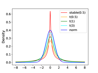
Figure 1: Probability density function (PDF) of normal distribution, 0.5-stable distribution, and Student’s $t$-distribution with df = 0.5, 1, and 3.

Note that the smaller the $\alpha$, the heavier the tail. Figure 1 shows several examples of the $\alpha$-heavy-tail noise. In particular, for a Cauchy random (Student’s $t$-distribution with $\text{df}=1$.) variable $\eta$ with PDF, $f(x)=\frac{1}{\pi}\cdot\frac{1}{1+x^{2}}$, $\alpha=1$; for a Student’s $t(\text{df})$-distribution with PDF, $f(x)=\frac{1}{\sqrt{\text{df}}\cdot\text{B}(\frac{1}{2},\frac{\text{df}}{2})}\cdot(1+\frac{x^{2}}{\text{df}})^{-\frac{\text{df + 1}}{2}}$, $\alpha=\text{df}$. The asymptotic behavior of $\alpha$-stable distribution is described by $f(x)\sim\frac{1}{|x|^{\alpha+1}}$, which shows that $\alpha$-stable distribution also has the $\alpha$-heavy tail. We also point out that normal distribution is not $\alpha$-heavy tail for any finite $\alpha$.

Note that the symmetry assumption in the noise distribution is necessary. For $\alpha<1$, the mean of $\eta$ is not necessarily existential. Hence, symmetry is needed for the problem to be well-defined. We note that for $\alpha>1$, we can relax the assumption of symmetry by simply assuming $\mathbb{E}[\eta]=0$. For the sake of presentation, we assume symmetry through out.

In comparison with existing literature, we require no assumptions on the bound or sub-Gaussianity of $\eta$, e.g., in (Abbasi-Yadkori et al., 2011). Meanwhile, we also impose no restrictions on the existence of the $(1+\epsilon)$-th moment of the noise, which is required in Bubeck et al. (2013); Medina and Yang (2016); Shao et al. (2018); Xue et al. (2020). Indeed, the $\alpha^{\prime}$-th moment of $\eta$ for any $\alpha^{\prime}<\alpha$ does exist. However, when $\alpha\leq 1$, previous algorithms fail to guarantee a sub-linear regret bound.

3 Robust Estimator for Super Heavy-tailed Noises

To introduce our estimator, we first briefly review previous robust estimators and provide some motivations of designing a new robust estimator. For rest of the section, we consider i.i.d. copies of random variable $X=x+\eta$, where $x$ is a fixed number and $\eta$ is a symmetric noise. Consider a sequence of $\widetilde{n}$ i.i.d. copies of $X$: $X_{1},X_{2},\cdots,X_{\widetilde{n}}$. There are two notable robust estimators for estimating $x$ in the heavy-tail setting.

The first robust estimator is the truncated empirical mean estimator, selects the random variables with magnitude smaller than certain threshold $c>0$ and computes the empirical mean after selection:

$$\widehat{\mu}_{1}=\frac{1}{\widetilde{n}}\sum_{i=1}^{\widetilde{n}}X_{i}1_{\{|X_{i}|\leq c\}}.$$ (3.1)

The second one is called the median of means, which is defined as follows,

$$\widehat{\mu}_{2}=\text{median}\Bigl{(}\Big{\{}\frac{1}{k}\sum_{i=1}^{k}X_{(j-1)k+i}\Big{\}}_{j=1}^{k^{\prime}}\Bigr{)},$$ (3.2)

where $k$ is a parameter to be decided.

Unfortunately, as shown in Bubeck et al. (2013), these two robust estimators critically rely on the existence of mean of the random noise, and hence cannot be applied to super heavy-tailed noise with no mean. Indeed, the truncated random variable can significantly distort the center whereas the median of means estimator does not concentrate enough. We illustrate in more detail in Section 3.3 about their performance. Thus, for $\alpha$-heavy-tail random variables with $\alpha<1$, new robust estimators are needed to effectively handle such noise.

3.1 Mean of Medians

The fundamental reason of the failure of the above estimators is due to the requirement of the existence of mean in the noise. To resolve this issue, we propose to use the empirical median, which is super robust against heavy tails as it characterizes the properties of the distribution, instead of moments. For instance, no matter how heavy the tail of the noise is, as long as it has certain probability of being close to $0$, the median will have high probability being close to $0$.

To leverage the above observation, we propose a novel statistical estimator: mean of medians (mom). Specifically, we split the $\widetilde{n}$ samples into $k^{\prime}$ blocks and takes the mean of the median in each block. For $\widetilde{n}$ i.i.d. symmetric random variables $X_{1},X_{2},\cdots,X_{\widetilde{n}}$, we define the mean of medians estimator by

$$X_{\text{mom}}=\frac{1}{k^{\prime}}\sum_{j=1}^{k^{\prime}}\text{median}(X_{(j-1)k+1},X_{(j-1)k+2},\cdots,X_{jk}),$$ (3.3)

where $k=\lceil\widetilde{n}^{\varepsilon}\rceil$ and $k^{\prime}=\lfloor\widetilde{n}/k\rfloor$. Here $\varepsilon\in(0,1)$ is a parameter depends $\epsilon$ and will be specified later.

3.2 Theoretical Guarantees of Mean of Medians Estimator

In this subsection, we provide the theoretical guarantees for the mean of medians estimator. First, we have the following lemma, which characterizes the median of heavy-tailed noises.

Lemma 3.1.

Let $X_{1},X_{2},\cdots,X_{m}$ be $m$ i.i.d. symmetric random variables satisfying $\Pr(|X_{i}|>y)\leq\frac{1}{y^{\alpha}}$. Suppose $Y$ is the median of $X_{1},X_{2},\cdots,X_{m}$, we have

$$\Pr(|Y|\leq 4^{1/\alpha})\geq 1-2e^{-m/8}.$$

Proof.

First, we define the random variables $\widehat{X_{i}}=1_{\{|X_{i}|>4^{1/\alpha}\}}$ for $i\in[m]$. By the fact that $\Pr(|X_{i}|>y)\leq\frac{1}{y^{\alpha}}$, we have $p_{i}=\Pr(\widehat{X_{i}}=1)\leq 1/4$. Together with Hoeffding’s inequality, we obtain

$$\Pr\left(\sum_{i=1}^{m}\widehat{X}_{i}\geq m/2\right)\leq\Pr\left(\sum_{i=1}^{m}\widehat{X}_{i}-p_{i}\geq m/4\right)\leq e^{-m/8}.$$

Note that the median $Y$ satisfies $Y>4^{1/\alpha}$ if and only if at least half of the estimates $X_{i}$ are above $4^{1/\alpha}$, which is equivalent to $\Pr(\sum_{i=1}^{m}\widehat{X}_{i}\geq m/2)$. Hence, we have $Y>4^{1/\alpha}$ with probability at most $e^{-m/8}$. Similarly, we can obtain that $Y<4^{1/\alpha}$ with probability at most $e^{-m/8}$. Thus, it holds that

$$\Pr(|Y|>4^{1/\alpha})\leq 2e^{-m/8},$$

which concludes the proof of Lemma 3.1. ∎

Lemma 3.1 shows that, when the number of samples $m$ is large, the median of $m$ i.i.d. super heavy tailed noise random variables is bounded by $4^{1/\alpha}$ with high probability. Equipped with this lemma, we formally describe the main results for the mean of medians estimator as follows.

Theorem 3.2.

Let $\varepsilon,\alpha>0$ be parameters. Let $X_{1},X_{2},\cdots,X_{\widetilde{n}}$ be $\widetilde{n}$ i.i.d. symmetric $\alpha$-heavy-tail random variables. When $\widetilde{n}\geq\max\{C,\big{(}16\log(2/\delta)\bigr{)}^{1/\varepsilon}\}$, for the mean of medians estimator defined in (3.3), we have

$$\mathbb{E}[X_{\text{mom}}]=0,\qquad\text{and}\quad|X_{\text{mom}}|\leq\sqrt{\frac{2\cdot 4^{2/\alpha}}{\widetilde{n}^{1-\varepsilon}}\cdot\log(4/\delta)}$$

with probability $1-\delta$. Here $C$ is a constant depending on $\varepsilon$ such that $2C^{1-\varepsilon}e^{-C^{\varepsilon}/16}\leq 1$.

Proof.

To facilitate our analysis, we denote the median of $(X_{(j-1)k+1},X_{(j-1)k+2},\cdots,X_{jk})$ by $Y_{j}$. Here $k=\lceil\widetilde{n}^{\varepsilon}\rceil$ and $k^{\prime}=\lfloor\widetilde{n}/k\rfloor$. Under this notation, by Lemma 3.1, we obtain that

$$\Pr(|Y_{j}|\leq 4^{1/\alpha})\geq 1-2e^{-k/8}$$ (3.4)

for any $j\in[k^{\prime}]$. Let $Z_{j}=Y_{j}\cdot{\bf 1}_{\{|Y_{j}|\leq 4^{1/\alpha}\}}$, we have

$$\Pr(|X_{\text{mom}}|>t) =\Pr\Bigl{(}\Big{|}\frac{1}{k^{\prime}}\sum_{j=1}^{k^{\prime}}Y_{j}\Big{|}>t\Bigr{)}$$

$$\leq\Pr\Bigl{(}\Big{|}\frac{1}{k^{\prime}}\sum_{j=1}^{k^{\prime}}Z_{j}\Big{|}>t\Bigr{)}+\sum_{j=1}^{k^{\prime}}\Pr(|Y_{j}|>4^{1/\alpha})$$

$$\leq 2\exp\Big{(}-\frac{k^{\prime}t^{2}}{2\cdot 4^{2/\alpha}}\Big{)}+2k^{\prime}e^{-k/8},$$

where the last inequality follows from Hoeffding’s inequality and Equation (3.4). When choosing

$$\widetilde{n}\geq\max\{C,\big{(}16\log(2/\delta)\bigr{)}^{1/\varepsilon}\},$$

where $C$ is a sufficient large constant depending on $\varepsilon$ such that $2C^{1-\varepsilon}e^{-C^{\varepsilon}/16}\leq 1$, we have that $2k^{\prime}e^{-k/8}\leq\delta/2$. Hence, by setting $t=\sqrt{\frac{2\cdot 4^{2/\alpha}}{\widetilde{n}^{1-\varepsilon}}\cdot\log(4/\delta)}$, we have

$$|X_{\text{mom}}|\leq\sqrt{\frac{2\cdot 4^{2/\alpha}}{\widetilde{n}^{1-\varepsilon}}\cdot\log(4/\delta)}$$

with probability at least $1-\delta$. Together with the fact that the noise is symmetric, we conclude the proof of Theorem 3.2. ∎

Remark 3.3 (Sample Complexity).

Solving the inequality $|X_{\text{mom}}|\leq\zeta$ gives that $\widetilde{n}\geq\bigl{(}\frac{2\cdot 4^{2/\alpha}}{\zeta^{2}}\cdot\log(4/\delta)\bigr{)}^{\frac{1}{1-\varepsilon}}$. Together with the constraint that $\widetilde{n}\geq\max\{C,(16\log(2/\delta))^{1/\varepsilon}\}$, we have $\widetilde{n}\geq\max\{C,(16\log(2/\delta))^{1/\varepsilon},\bigl{(}2\cdot\frac{4^{2/\alpha}}{\zeta^{2}}\cdot\log(4/\delta)\bigr{)}^{\frac{1}{1-\varepsilon}}\}$. If we choose $\varepsilon$ near to $0$, $C$ and $(16\log(2/\delta))^{1/\varepsilon}$ are large. If we choose $\varepsilon$ near to $1$, $\bigl{(}\frac{2\cdot 4^{2/\alpha}}{\zeta^{2}}\cdot\log(4/\delta)\bigr{)}^{\frac{1}{1-\varepsilon}}$ is large. In other words, there is a trade-off in $\varepsilon$ to balance these three terms.

3.3 Comparison with Previous Robust Estimators

Coming back to the other robust estimators, truncated empirical mean and median of means have good guarantees when the mean of the random variables exist. Let us consider $\widetilde{n}>0$ i.i.d. random variables $\{X_{1},X_{2},\cdots,X_{\widetilde{n}}\}$ and follow the notation in Bubeck et al. (2013). Specifically, suppose $X_{i}$ satisfies that

$$\mathbb{E}[X_{i}]=\mu,\quad\text{and}\quad\mathbb{E}[|X_{i}-\mu|^{1+\epsilon}]\leq v,\quad\forall i\in[\widetilde{n}]$$

for some $\epsilon\in(0,1)$. Bubeck et al. (2013) shows that, when we set $c$ and $k$ properly in (3.1) or (3.2), we have

$$|\mu-\widehat{\mu}|\lesssim v^{\frac{1}{1+\epsilon}}\Bigl{(}\frac{C(\epsilon)\log(1/\delta)}{\widetilde{n}}\Bigr{)}^{\frac{\epsilon}{1+\epsilon}},$$ (3.5)

where $\widehat{\mu}$ is an estimator computed by (3.1) or (3.2). On the other hand, by Theorem 3.2, we have that the mean of medians estimator has an error rate of $\widetilde{O}(1/\widetilde{n}^{\frac{1-\varepsilon}{2}})$. In what follows, we compare the mean of medians estimator with previous robust estimators throughout two regimes of $\epsilon$.

• When $\epsilon\leq 0$ , truncated empirical mean and median of means are not valid any more. In contrast, our estimator can still tackle such heavy tailed random variables.

• When $0<\epsilon<1$, by choosing $\varepsilon<\frac{1-\epsilon}{1+\epsilon}$ in (3.3), we know that mean of medians enjoys the convergence rate $\widetilde{O}(1/\widetilde{n}^{\frac{1-\varepsilon}{2}})$, which is better than the rate $\widetilde{O}(1/\widetilde{n}^{\frac{\epsilon}{1+\epsilon}})$ of truncated empirical mean and median of means.

For heavy tailed linear bandits, we mainly focus on the setting where $\epsilon<1$ because Bubeck et al. (2013) proposes a nearly optimal algorithm with $O(\sqrt{T})$ regret when the noises have finite variance ($\epsilon\geq 1$). Therefore, we can conclude that our mean of medians estimator are preferable than previous robust estimator for heavy tailed linear bandits (especially for the super heavy-tailed linear bandits).

4 Generic Algorithmic Framework for Super Heavy-Tailed Linear Bandits

4.1 A Generic Bandit Algorithm

In this section, we propose a new algorithmic framework for the super heavy-tailed linear bandits defined in Definition 2.1. Specifically, by utilizing mean of medians (Algorithm 2) as a subroutine, we can transform any existing algorithm, e.g., (Dani et al., 2008; Rusmevichientong and Tsitsiklis, 2010; Abbasi-Yadkori et al., 2011; Soare et al., 2014; Jedra and Proutiere, 2020), into an efficient algorithm for super heavy-tailed linear bandits. The procedure is rather basic: the outer algorithm simply collects rewards of an arm and pass them into the mean of medians estimator, and use the output value as a new reward, which will have a light tail (by Theorem 3.2). The details are given in Algorithm 1.

Algorithm 1 Synthetic Algorithm

1:  Input: A bandit algorithm $\mathcal{A}$, $\delta>0$, $\varepsilon>0$ and an integer $\widetilde{n}$.

2:  for $t=1,2,\cdots$ do

3:     Algorithm $\mathcal{A}$ chooses the arm $x_{t}$.

4:     Receive the reward $r_{t}\leftarrow$ Mean of Medians$(x_{t},\widetilde{n},\varepsilon)$. (Algorithm 2)

5:  end for

Algorithm 2 Mean of Medians

1:  Input: An arm $y$ and an integer $\widetilde{n}$, and a parameter $\varepsilon\in(0,1)$.

2:  Set $k=\lceil{\widetilde{n}}^{\varepsilon}\rceil$ and $k^{\prime}=\lfloor{\widetilde{n}}/k\rfloor$.

3:  Pull the arm $y$ for $\widetilde{n}$ times and obtain the corresponding rewards $r_{1},r_{2},\cdots,r_{\widetilde{n}}$.

4:  Let $Y_{j}$ be the median of $\{r_{(j-1)k+1},r_{(j-1)k+2},\cdots,r_{jk}\}$ for $j\in[k^{\prime}]$.

5:  Set $r=\frac{1}{k^{\prime}}\sum_{j=1}^{k^{\prime}}Y_{j}$.

6:  return  $r$.

4.2 Theoretical Guarantees

In this subsection, we establish theoretical guarantees for our algorithmic framework (Algorithm 1).

Theorem 4.1 (Regret Minimization).

Suppose a linear bandit instance, $(\mathcal{X},\theta)$, has $\alpha$-heavy-tail noise for some $\alpha>0$. Fix $\varepsilon\in(0,1)$. Let $\widetilde{n}=\lceil\max\{C,\big{(}16\log(2T/\delta)\bigr{)}^{1/\varepsilon},(2\cdot 4^{2/\alpha}\log(4/\delta))^{\frac{1}{1-\varepsilon}}\}\rceil$, $C$ is a constant depending on $\varepsilon$ such that $2C^{1-\varepsilon}e^{-C^{\varepsilon}/16}\leq 1$ in Algorithm 1. Let $\mathcal{A}$ be a linear bandit algorithm, which achieves regret bound $R(d,T,\delta)$ under $1$-sub-Gaussian noises with probability at least $1-\delta$. Then, Algorithm 1 with input $(\mathcal{A},\delta,\varepsilon,\widetilde{n})$ enjoys a regret bound

$$\widetilde{n}\cdot R(d,T/\widetilde{n},\delta)$$

with probability at least $1-2\delta$.

Proof.

Fix $T>0$. We divide total $T$ steps into $\widetilde{T}=\lfloor T/\widetilde{n}\rfloor$ blocks, each of which consists of $\widetilde{n}$ steps. With each block, we pull an arm for $\widetilde{n}$ times. For $t$-th block, we assume that $r_{t}=\theta^{\top}x_{t}+\eta_{t}$. By Theorem 3.2, for any $t\in[T]$, we have

$$\mathbb{E}[\eta_{t}]=0,\quad\text{and}\quad|\eta_{t}|\leq 1$$

with probability at least $1-\delta/T$. Thus, we reduce the super heavy tailed linear bandits into linear bandits with $1$-sub-Gaussian noises. Together with our assumption that $\mathcal{A}$ achieves regret $R(d,T,\delta)$ for the $1$-sub-Gaussian linear bandits with probability at least $1-\delta$, we have

$$\text{Regret}(T)\leq\widetilde{n}\cdot R(d,T/\widetilde{n},\delta),$$

with probability at least $1-2\delta$, which concludes the proof of Theorem 4.1. ∎

Remark 4.2.

The parameter $\alpha$ does not need to be known exactly. Any lower bound of the true $\alpha$ suffices to ensure the same guarantee. It can also be treated as a hyper parameter in the algorithm.

Remark 4.3.

Shao et al. (2018); Xue et al. (2020) establish an expected regret lower bound $\Omega(T^{\frac{1}{1+\epsilon}})$ for the linear bandits with heavy-tailed payoffs, where the payoffs admit finite $1+\epsilon$ moments for some $\epsilon\in(0,1]$. This is not inconsistent with our conclusion since we consider the pseudo regret instead of the expected regret. Moreover, it is reasonable to consider the pseudo regret since we cannot define the expected regret when the mean of the noise does not exist.

Remark 4.4.

Note that for any fixed $\alpha>0$, $\widetilde{n}$ is only logarithmically depending on $T$. Hence the overall regret bound is only a factor of $\mathrm{poly}\log(T)$ worse compared to the light tail counterpart. If algorithm $\mathcal{A}$ obtains a near-optimal regret for sub-Gaussian noise (e.g., algorithms in Abbasi-Yadkori et al. (2011)), then our regret bound is near optimal for $\alpha$-heavy-tail noise as well. To instantiate Algorithm 1, we apply the near-optimal algorithm in Abbasi-Yadkori et al. (2011), and immediately obtain the following near-optimal regret bound.

Corollary 4.5.

Suppose a linear bandit instance, $(\mathcal{X},\theta)$, has $\alpha$-heavy-tail noise for some $\alpha>0$. We use the OFUL algorithm in Abbasi-Yadkori et al. (2011) as the input in Algorithm 1 and set $\varepsilon=1/2$. Let $\widetilde{n}=\lceil\max\{C,\big{(}16\log(2T/\delta)\bigr{)}^{2},(2\cdot 4^{2/\alpha}\log(4/\delta))^{2}\}\rceil$, where $C$ is a constant such that $2\sqrt{C}e^{-\sqrt{C}/16}\leq 1$ in Algorithm 1. Then, by using Algorithm 1 achieves a regret bound $\widetilde{O}(d\sqrt{\widetilde{n}T}\log(T/\delta))$ with probability at least $1-\delta$.

5 Experiment

In this section, we conduct numerical experiments to demonstrate the effectiveness of our algorithmic framework for super heavy-tailed linear bandit problems. Experiments are run in a Windows 10 laptop with Intel(R) Core(TM) i7-8750H CPU and 16GB memory.

We adopt state-of-the-art algorithms, i.e., SupBMM and SupBTC, proposed by Xue et al. (2020) as the input algorithm $\mathcal{A}$ in Algorithm 1, yielding synthetic algorithms SupBMM_mom and SupBTC_mom respectively. Here “mom” means using our mean of medians estimator to process noise as in Algorithm 1. Apart from SupBMM and SupBTC of Xue et al. (2020), we also make comparisons with MoM and CRT of Medina and Yang (2016), MENU and TOFU of Shao et al. (2018). All the traditional algorithms require moments condition, i.e., for some $\epsilon\in(0,1]$, $(1+\epsilon)$-th central moment of the heavy-tailed noise is bounded under some $v>0$.

For comparison, we show cumulative regret with respect to number of rounds of bandits played over a fixed finite-arm decision set $\mathcal{X}$. We generate 10 independent paths for each algorithms and show the average cumulative regret. We use the following experimental setup corresponding to that in Medina and Yang (2016); Xue et al. (2020). Let the feature dimension $d=10$, the number of arms $|\mathcal{X}|=K=20$. For the chosen arm $x_{t}\in\mathcal{X}$, reward is $\theta^{*\top}x_{t}+\eta_{t}$, where $\theta^{*}=\mathbf{1}_{d}/\sqrt{d}\in\mathbb{R}^{d}$ so that $\|\theta^{*}\|_{2}=1$ and $\eta_{t}$ is sampled from a Student’s $t$-distribution with degree of freedom df as a parameter to be specified. Every contextual information of time $t$, i.e., $x_{t,a},a\in[K]$ , is sampled from uniform distribution of $[0,1]$ respectively for each dimension, with normalization made to ensure $\|x_{t,a}\|_{2}=1$.

This section is divided into 2 parts: First, we choose an environment with heavy-tailed noise, whose $(1+\epsilon)$-th central moment is finite for some $\epsilon\in(0,1]$. Student’s $t$-noises with $\text{df}\in\{3,1.02\}$ are chosen, whose moment parameter $\epsilon\in\{1,0.01\}$ and bound parameter $v\in\{3,65.19\}$ respectively. Then we consider linear bandits with super heavy-tailed noise. Student’s $t$-noises with $\text{df}\in\{1,0.5\}$ are chosen. In this setting, $(1+\epsilon)$-th central moment no longer exists for any $\epsilon\geq 0$. In theory, none of the algorithms mentioned above could work properly. In order to make other algorithms work, we input $\epsilon=0.01$ and treat $v$ as a hyper parameter that needs to be tuned for relatively good performance. We remark that Algorithm 1 is relatively not sensitive to the choice of $v$ (See appendix).

Our algorithm’s parameter $\varepsilon$ is set to $0.5$ since results vary little with $\varepsilon$ empirically (See appendix for more information). And $\widetilde{n},k,k^{\prime}$ is set according to Theorem 4.1 and Algorithm 2. For the noise processed by our mean of medians estimator (Algorithm 2), we input $\epsilon=1$ and tune $v$ to ensure the performance of Algorithm 1. Specifically, no matter how heavy-tailed original noise is, our mean of medians estimator can reduce super heavy-tailed noise to bounded noise with high probability, as is shown in Theorem 3.2. So it is reasonable to assume the processed noise has a finite second moment, which is bounded by an unknown $v$ to be tuned, i.e. $\mathbb{E}[|\eta_{\text{mom}}|^{2}]\leq v$.

Figure 2: Comparison of our algorithms versus MoM, CRT, MENU, TOFU, SupBMM and SupBTC in heavy-tailed linear bandit problems for $1\times 10^{4}$ rounds.

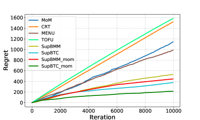
(a) Student’s $t$-Noise with $\text{df}=3$

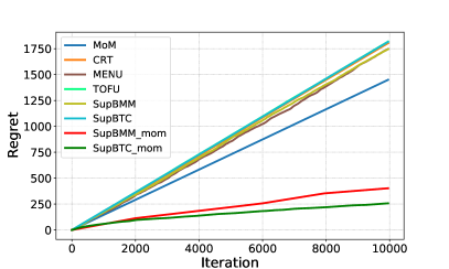
(b) Student’s $t$-Noise with $\text{df}=1.02$

We show experimental results of heavy-tailed linear bandit problems in Figure 2 for $1\times 10^{4}$ rounds. Figure 2(a) compares our algorithms with the aforementioned six algorithms under Student’s $t$-noise with $\text{df}=3$, which corresponds to the results in Xue et al. (2020). Figure 2(b) presents regret versus iteration with $\text{df}=1.02$. In Figure 2(b), our algorithms outperform MoM, CRT, MENU, TOFU, SupBMM and SupBTC with heavy-tailed noise as expected. Specially, in Figure 2(b), $\text{df}=1.02$, so $1.01$-th central moment exists, which is bounded by a rather big number $v=65.19$. In this setting, all of other algorithms perform poorly, whereas our algorithms work perfectly well, which verifies effectiveness of our algorithms as in Section 3.3 and Theorem 4.1.

Figure 3: Comparison of our algorithms versus MoM, CRT, MENU, TOFU, SupBMM and SupBTC in super heavy-tailed linear bandit problems for $1\times 10^{4}$ rounds.

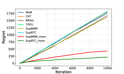
(a) Student’s $t$-Noise with $\text{df}=1$

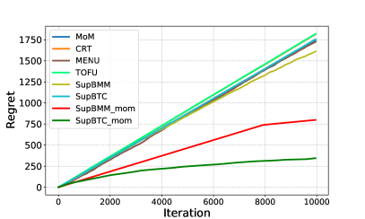
(b) Student’s $t$-Noise with $\text{df}=0.5$

Experimental results of super heavy-tailed linear bandit problems are demonstrated in Figure 3 for $1\times 10^{4}$ rounds. Figure 3(a) and (b) consider $\text{df}=1,0.5$ respectively. As is shown in Figure 3, our algorithms perform significantly better than other algorithms. And SupBTC_mom performs better than SupBMM_mom.

In a word, our algorithms outperform the state-of-the-art algorithms even when $\epsilon>0$, and have comparably good performance when $\epsilon\leq 0$, which is consistent with the theoretical results in Theorem 4.1.

6 Conclusion

In this work, we have proposed a generic algorithmic framework for super heavy-tailed linear bandits. Such an algorithmic framework incorporates a classical linear bandit algorithm to tackle existing challenges such as the trade-off between exploration and exploitation, and more importantly, adopts the mean of medians estimator to handle the challenge of super heavy-tailed noises. We show that our algorithmic framework is provably efficient for regret minimization. Meanwhile, we conducted numerical experiments to validate the effectiveness of our framework in practice. To the best of our knowledge, we make the first attempt to study the super heavy-tailed linear bandits and propose the first provably efficient method that successfully handles super heavy-tailed noises.

7 Acknowledgments

The authors would like to thank anonymous reviewers for their valuable advice. Part of the work was done while Han Zhong and Jiayi Huang were students in University of Science and Technology of China. This work was supported by National Key R$\&$D Program of China (2018YFB1402600), Key-Area Research and Development Program of Guangdong Province (No. 2019B121204008), BJNSF (L172037) and Beijing Academy of Artificial Intelligence. Project 2020BD006 supported by PKU-Baidu Fund.

Appendix A Additional Experimental Results

This section provides additional experimental results of Section 5.

Figure 4: Comparison of our algorithms versus MoM, CRT, MENU, TOFU, SupBMM and SupBTC under Student’s $t$-Noise with $\text{df}=3$. The figures at the bottom of each subfigure represent estimation error $\|\widehat{\theta}_{t}-\theta^{*}\|_{2}/\|\theta^{*}\|_{2}$, except for SupBMM and SupBTC since $\widehat{\theta}_{t}$ is not available.

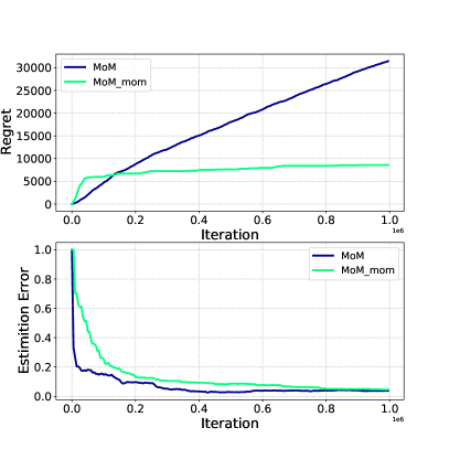
(a) MoM

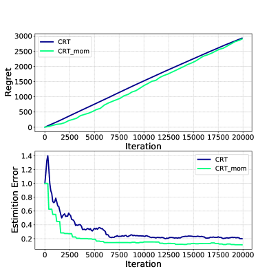
(b) CRT

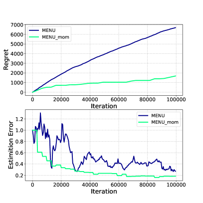
(c) MENU

(d) TOFU

(e) SupBMM

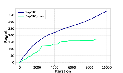
(f) SupBTC

Figure 5: Comparison of our algorithms versus MoM, CRT, MENU, TOFU, SupBMM and SupBTC under Student’s $t$-Noise with $\text{df}=1.02$. The figures at the bottom of each subfigure represent estimation error $\|\widehat{\theta}_{t}-\theta^{*}\|_{2}/\|\theta^{*}\|_{2}$, except for SupBMM and SupBTC since $\widehat{\theta}_{t}$ is not available.

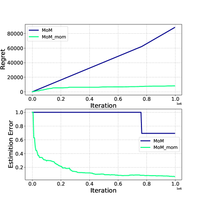
(a) MoM

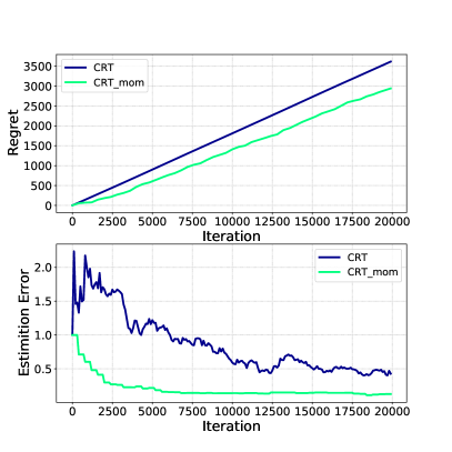
(b) CRT

(c) MENU

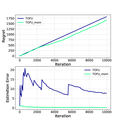
(d) TOFU

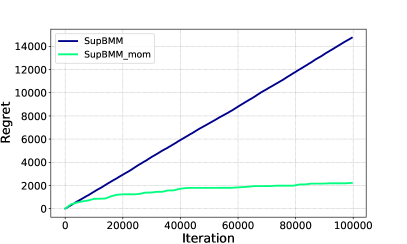
(e) SupBMM

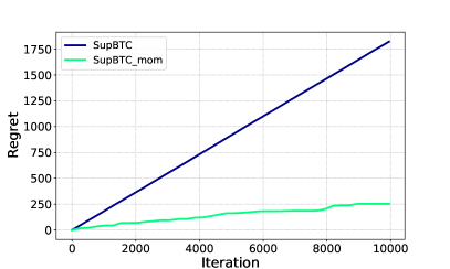
(f) SupBTC

Figure 4 and 5 try to explain the reason why our algorithms have much better performance than the other algorithms in super heavy-tailed linear bandit problems. For every algorithm from MoM, CRT, MENU, TOFU, SupBMM and SupBTC, we transform it into an efficient algorithm for super heavy-tailed linear bandits by Algorithm 1. The counterpart is named as the original name with suffix “_mom”, which represents our mean of medians estimator. Figure 4 considers Student’s $t$-noise with $\text{df}=3$ while Figure 5 focuses on more heavy-tailed case, where $\text{df}=1.02$. We notice that in Figure 4, when $\text{df}=3$, all algorithms make an accurate estimation of $\theta^{*}$, thus perform well. However, in Figure 5, when $\text{df}=1.02$, the estimation error of other algorithms seems to vary more and even not converge. While the counterparts by our algorithmic framework have estimation error approaching $0$ stably. In this way, no matter how heavy-tailed the noise is, as long as we choose $\widetilde{n}$ large enough according to Theorem 4.1, our algorithms will have comparably good performance.

What’s more, we notice that in Figure 5, performance improvement varies with different algorithms. For example, if we take TOFU and MENU as input algorithm $\mathcal{A}$ in Algorithm 1 respectively, the performance of TOFU_mom is not as good as MENU_mom, even TOFU and MENU have comparable performance. In this way, we only adopt SupBMM_mom and SupBTC_mom for comparisons in Figure 2 for better performance.

Appendix B The Selection of Parameter $\varepsilon$

In this section, we further illustrate the selection of parameter $\varepsilon$.

First we discuss the choice of $\varepsilon$ with respect to $\alpha$. In order to approximate the optimal value of $\varepsilon$, according to Theorem 4.1, we let $\big{(}16\log(2T/\delta)\bigr{)}^{1/\varepsilon}=(2\cdot 4^{2/\alpha}\log(4/\delta))^{\frac{1}{1-\varepsilon}}$. Figure 6 shows the relationship between $\varepsilon$ and $\alpha$, where we set $\delta=0.01$ and $T=10000$.

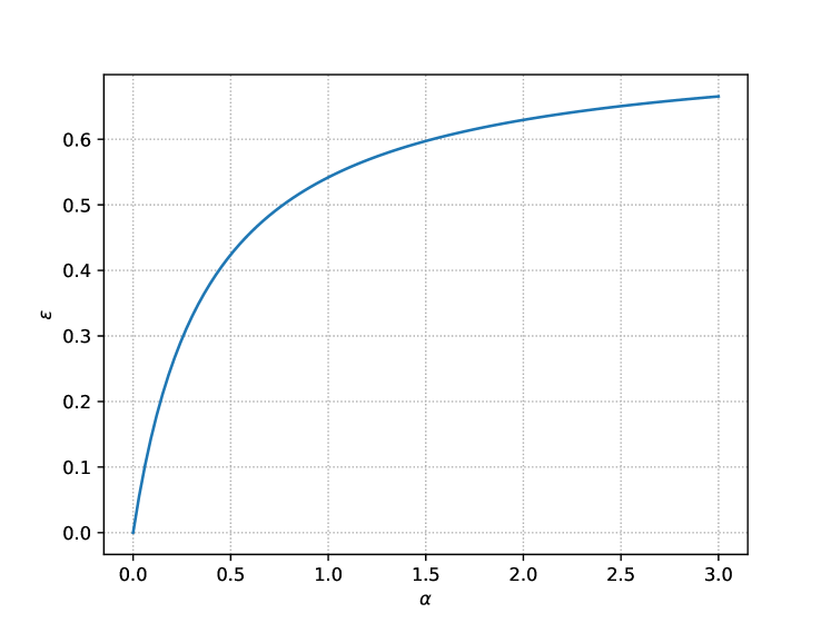
Figure 6: Optimal $\varepsilon$ with respect to $\alpha$.

Then we concern about how sensitive our mom-algorithms are to the choice of $\varepsilon\in(0,1)$. Figure 7 demonstrates the mean regret of 100 independent paths under Student’s $t$-noise with $\text{df}=1(\alpha=1)$, which corresponds to the setting of Figure 3(a) in our paper. Each sample path contains $10000$ iterations. We choose $\varepsilon\in[0.3,0.8]$ to avoid extreme situation, i.e. we can’t choose $\varepsilon$ close to $0$ or $1$.

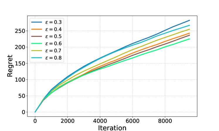
Figure 7: Mean regret of $100$ independent paths under Student’s $t$-noise with $\text{df}=1$ by algorithm SupBTC_mom.

We observe that the optimal $\varepsilon$ is between $0.5$ and $0.6$, which is consistent with the result in Figure 6.

Appendix C The Selection of Parameter $v$

In the experiments, for the noise processed by our mean of medians estimator, we choose to tune the bound parameter $v$ satisfying $\mathbb{E}[|\eta_{\text{mom}}|^{2}]\leq v$ to ensure performance. In this section, we show that our algorithms are not sensitive to $v$ according to the plots.

Additional plots are provided here for further illustration. Under the same setting of Section 5, multiple independent paths are generated by algorithm SupBTC_mom and SupBTC_mom respectively. Figures 8 and 9 shows the mean and median regret of $500$ independent paths under Student’s $t$-noise with $\text{df}=0.5$. Each sample path contains $10000$ iterations. And three values of parameter $v$ are selected over a suitably large range. Figure 8 is for algorithm SupBMM_mom and Figure 9 is for SupBTC_mom.

Figure 8: Mean and median regret of $500$ independent paths under Student’s $t$-noise with $\text{df}=0.5$ by algorithm SupBMM_mom.

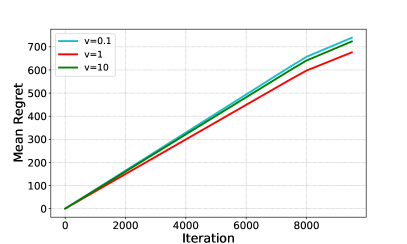
(a) Mean regret

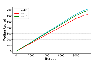
(b) Median regret

Figure 9: Mean and median regret of $500$ independent paths under Student’s $t$-noise with $\text{df}=0.5$ by algorithm SupBTC_mom.

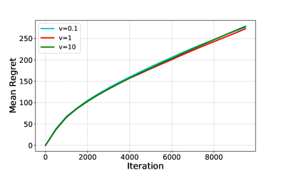
(a) Mean regret

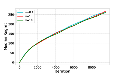
(b) Median regret

References

- Abbasi-Yadkori et al. [2011] Yasin Abbasi-Yadkori, Dávid Pál, and Csaba Szepesvári. Improved algorithms for linear stochastic bandits. In NIPS, volume 11, pages 2312–2320, 2011.
- Abe and Long [1999] Naoki Abe and Philip M Long. Associative reinforcement learning using linear probabilistic concepts. In ICML, pages 3–11. Citeseer, 1999.
- Auer [2002] Peter Auer. Using confidence bounds for exploitation-exploration trade-offs. Journal of Machine Learning Research, 3(Nov):397–422, 2002.
- Bubeck and Cesa-Bianchi [2012] Sébastien Bubeck and Nicolo Cesa-Bianchi. Regret analysis of stochastic and nonstochastic multi-armed bandit problems. arXiv preprint arXiv:1204.5721, 2012.
- Bubeck et al. [2013] Sébastien Bubeck, Nicolo Cesa-Bianchi, and Gábor Lugosi. Bandits with heavy tail. IEEE Transactions on Information Theory, 59(11):7711–7717, 2013.
- Chu et al. [2011] Wei Chu, Lihong Li, Lev Reyzin, and Robert Schapire. Contextual bandits with linear payoff functions. In Proceedings of the Fourteenth International Conference on Artificial Intelligence and Statistics, pages 208–214. JMLR Workshop and Conference Proceedings, 2011.
- Combes et al. [2017] Richard Combes, Stefan Magureanu, and Alexandre Proutiere. Minimal exploration in structured stochastic bandits. arXiv preprint arXiv:1711.00400, 2017.
- Cont and Bouchaud [2000] Rama Cont and Jean-Philipe Bouchaud. Herd behavior and aggregate fluctuations in financial markets. Macroeconomic dynamics, 4(2):170–196, 2000.
- Dani et al. [2008] Varsha Dani, Thomas P Hayes, and Sham M Kakade. Stochastic linear optimization under bandit feedback. 2008.
- Fiez et al. [2019] Tanner Fiez, Lalit Jain, Kevin Jamieson, and Lillian Ratliff. Sequential experimental design for transductive linear bandits. arXiv preprint arXiv:1906.08399, 2019.
- Garivier and Kaufmann [2016] Aurélien Garivier and Emilie Kaufmann. Optimal best arm identification with fixed confidence. In Conference on Learning Theory, pages 998–1027. PMLR, 2016.
- Hull [2012] John Hull. Risk management and financial institutions,+ Web Site, volume 733. John Wiley & Sons, 2012.
- Jedra and Proutiere [2020] Yassir Jedra and Alexandre Proutiere. Optimal best-arm identification in linear bandits. arXiv preprint arXiv:2006.16073, 2020.
- Lattimore and Szepesvari [2017] Tor Lattimore and Csaba Szepesvari. The end of optimism? an asymptotic analysis of finite-armed linear bandits. In Artificial Intelligence and Statistics, pages 728–737. PMLR, 2017.
- Lattimore and Szepesvári [2020] Tor Lattimore and Csaba Szepesvári. Bandit algorithms. Cambridge University Press, 2020.
- Li et al. [2010] Lihong Li, Wei Chu, John Langford, and Robert E Schapire. A contextual-bandit approach to personalized news article recommendation. In Proceedings of the 19th international conference on World wide web, pages 661–670, 2010.
- Li et al. [2016] Shuai Li, Alexandros Karatzoglou, and Claudio Gentile. Collaborative filtering bandits. In Proceedings of the 39th International ACM SIGIR conference on Research and Development in Information Retrieval, pages 539–548, 2016.
- Medina and Yang [2016] Andres Munoz Medina and Scott Yang. No-regret algorithms for heavy-tailed linear bandits. In International Conference on Machine Learning, pages 1642–1650. PMLR, 2016.
- Rachev [2003] Svetlozar Todorov Rachev. Handbook of Heavy Tailed Distributions in Finance: Handbooks in Finance, Book 1. Elsevier, 2003.
- Robbins [1952] Herbert Robbins. Some aspects of the sequential design of experiments. Bulletin of the American Mathematical Society, 58(5):527–535, 1952.
- Roberts et al. [2015] James A Roberts, Tjeerd W Boonstra, and Michael Breakspear. The heavy tail of the human brain. Current opinion in neurobiology, 31:164–172, 2015.
- Rusmevichientong and Tsitsiklis [2010] Paat Rusmevichientong and John N Tsitsiklis. Linearly parameterized bandits. Mathematics of Operations Research, 35(2):395–411, 2010.
- Shao et al. [2018] Han Shao, Xiaotian Yu, Irwin King, and Michael R Lyu. Almost optimal algorithms for linear stochastic bandits with heavy-tailed payoffs. arXiv preprint arXiv:1810.10895, 2018.
- Soare [2015] Marta Soare. Sequential resource allocation in linear stochastic bandits. PhD thesis, Université Lille 1-Sciences et Technologies, 2015.
- Soare et al. [2014] Marta Soare, Alessandro Lazaric, and Rémi Munos. Best-arm identification in linear bandits. arXiv preprint arXiv:1409.6110, 2014.
- Tao et al. [2018] Chao Tao, Saúl Blanco, and Yuan Zhou. Best arm identification in linear bandits with linear dimension dependency. In International Conference on Machine Learning, pages 4877–4886. PMLR, 2018.
- Xu et al. [2018] Liyuan Xu, Junya Honda, and Masashi Sugiyama. A fully adaptive algorithm for pure exploration in linear bandits. In International Conference on Artificial Intelligence and Statistics, pages 843–851. PMLR, 2018.
- Xue et al. [2020] Bo Xue, Guanghui Wang, Yimu Wang, and Lijun Zhang. Nearly optimal regret for stochastic linear bandits with heavy-tailed payoffs. arXiv preprint arXiv:2004.13465, 2020.