Abstract

Within an effective field theory method to general relativity, we calculate the fifth-order post–Newtonian (5PN) Hamiltonian dynamics also for the tail terms, extending earlier work on the potential contributions, working in harmonic coordinates. Here we calculate independently all (local) 5PN far-zone contributions using the in–in formalism, on which we give a detailed account. The five expansion terms of the Hamiltonian in the effective one body (EOB) approach, $q_{82},q_{63},q_{44},\bar{d_{5}}$ and $an$, can all be determined from the local contributions to the periastron advance $K^{\rm loc,h}(\hat{E},j)$, without further assumptions on the structure of the symmetric mass ratio, $\nu$, of the expansion coefficients of the scattering angle $\chi_{k}$. The $O(\nu^{2})$ contributions to the 5PN EOB parameters have been unknown in part before. We perform comparisons of our analytic results with the literature and also present numerical results on some observables.

1 Introduction

The discovery of gravitational wave signals from merging black holes and neutron stars [1] has been a recent milestone for general relativity and astrophysics. The different present and planned gravitational wave detectors are reaching higher and higher sensitivity [2], which requires more detailed predictions on the theoretical side than currently available. The motion of gravitating massive binary systems was studied perturbatively expanding in higher post–Newtonian (PN) orders right after the theory of general relativity has been found [3, 4]. Later on the corrections at 2PN [5], 3PN [6] and 4PN [7, 8, 9, 10, 11] have been calculated using a variety of techniques. First results at 5PN have been obtained in Refs. [12, 13, 14, 15, 16, 17] and at 6PN in Refs. [20, 18, 19]. In the Schwarzschild limit the contributions of $O(\nu^{0})$ are obtained to all post–Newtonian orders and the terms of $O(\nu)$ are know to $O(G_{N}^{21.5})$ [25, 26, 27] from the self–force formalism [28], where $G_{N}$ denotes Newton’s constant. The following kinematic variables are used

$$\nu=\frac{m_{1}m_{2}}{M^{2}}\in\left[0,\tfrac{1}{4}\right],\leavevmode\nobreak\ \leavevmode\nobreak\ \leavevmode\nobreak\ M=m_{1}+m_{2},\leavevmode\nobreak\ \leavevmode\nobreak\ \leavevmode\nobreak\ m_{1,2}=\frac{1}{2}M\left[1\pm\sqrt{1-4\nu}\right],\leavevmode\nobreak\ \leavevmode\nobreak\ \mu=M\nu,$$ (1)

where $m_{1}$ and $m_{2}$ are the two gravitating masses.

In this paper we complete the calculation of the 5PN corrections of the conservative dynamics for binary systems using an effective field theory (EFT) method [29, 4] and present main physical results. The calculation needs to be performed in $D=4-2\varepsilon$ dimensions because pole terms of $O(1/\varepsilon)$ are occurring in intermediate steps. One first considers gravity in $d=D-1$ integer spatial dimensions for all contributing pieces in the Lagrangian and then performs an analytic continuation. The multipole moments are dealt with in configuration space, while the graviton dynamics is calculated in momentum–space, after the post–Newtonian expansion has been performed via a Fourier–transform. Concerning the Feynman-diagrammatic representation of the far-zone contributions we follow Ref. [30] and extend it. The conservative Hamiltonian of the binary system, $H$, consists of the potential, $H_{\rm pot}$, and the far-zone terms involving back scattered radiation, $H_{\text{{rad}}}$, or can be likewise decomposed into the local, $H_{\rm loc}$, and non–local, $H_{\rm nl}$, contributions

$$H=H_{\rm pot}+H_{\text{{rad}}}=H_{\rm loc}+H_{\rm nl}.$$ (2)

We calculate the 5PN Hamiltonian ab initio starting with the path integral for classical gravity, for which a post–Newtonian expansion is performed by applying an EFT description [29, 4]. Methods originally developed for Quantum Field Theories are applied. About 190.000 Feynman diagrams contribute. They are generated by QGRAF [31]. Main parts of the calculation are performed using FORM [32]. The reduction to a very small set of master integrals is performed using Crusher [33] using the integration-by-parts relations [34]. The 5PN potential terms have been calculated by us in Ref. [16]. There we also described how the singularities in the potential and far-zone terms [7, 15, 19, 35, 36, 37, 38, 30] are canceling, together with an additional canonical transformation. The whole 5PN calculation is performed starting in the Lagrange formalism and finally deriving the Hamiltonian. Also the non–local 5PN contributions were presented, see also [15]. What remained to be calculated beyond the contributions given in [16] is a series of local far-zone contributions. These terms contribute at $O(\nu)$ and $O(\nu^{2})$. They are due to the 1PN correction to the electric quadrupole moment, written symbolically, $EQ_{ij}Q_{ji}$, with $E$ the energy, [38], the octupole moment, $EO_{ijk}O_{ijk}$, the magnetic quadrupole moment, $EJ_{ij}J_{ji}$, the angular momentum failed tail, $L_{k}\varepsilon_{ijk}Q_{il}Q_{jl}$, with $\vec{L}$ the angular momentum, and the memory terms, $Q_{ij}Q_{jk}Q_{ki}$, which have also been considered in Ref. [30]. These multipole contributions are calculated in $D$ dimensions starting with harmonic coordinates. As has been outlined in [30, 16] only the contributions involving two electric quadrupole, octupole, or magnetic quadrupole moments have poles of $O(1/\varepsilon)$ and receive logarithmic contributions. All other multipole moments can be calculated in $D=4$ dimensions and form rational contributions to the 5PN Hamiltonian. We have performed an independent calculation of these and related contributions and performed a detailed comparison with [30].

The Hamiltonian $H$ in Eq. (2) is gauge dependent and singular. To compare different approaches one has to either relate the Hamiltonians by canonical transformations or to compare the predictions for the resulting observables. This applies to the case of harmonic coordinates in the present approach and effective one body coordinates in [15]. In Ref. [15] different methods and constraints implied by the $\nu$-structure of the expansion coefficients of the scattering angle $\chi_{k}$, (48), have been used to construct the Hamiltonian and all but two $O(\nu^{2})$ parameters, $\bar{d}_{5}$ and $a_{6}$, were determined in this way for $H_{\rm EOB}$ up to 5PN.

In Ref. [16] we obtained all terms except the rational terms of $O(\nu^{2})$, the calculation of which we had not yet completed, as far as local far-zone contributions were concerned. For $\bar{d}_{5}$ and $a_{6}$ we have, more than in Ref. [15], obtained the $O(\nu^{2}\pi^{2})$ terms, which stem from the potential contributions. We remind that the magnetic quadrupole contribution necessitates a finite renormalization due to the analytic continuation of $\varepsilon_{ijk}$ in dimensional regularization, which implies the contribution $\delta_{J}H$, Eq. (61) in [16]. We observe the same finite renormalization in the $O(\nu)$ term for the binding energy and the local contribution to periastron advance $K^{\rm loc,h}(\hat{E},j)$, cf. [16]. Here ‘h’ stands for harmonic coordinates.

In the present paper we calculate the 5PN $O(\nu^{2})$ terms and perform a series of comparisons to the literature. In Section 2 we calculate the 5PN local far-zone terms. To compare with Ref. [15] we express our results for the local contributions obtained in the harmonic gauge in terms of effective one body (EOB) potentials in Section 3. To fix the five new EOB parameters at 5PN we are solely using the local contributions to periastron advance $K^{\rm loc,h}(\hat{E},j)$, which is an observable [44] since the non–local terms are known in explicit form via an eccentricity expansion, cf. [15, 16], and does not require any regularization. Furthermore, we will not use assumptions on the $\nu$ dependence of the observables used but perform a direct calculation within the framework of an effective field theory approach. The binding energy and periastron advance in the circular case are used for consistency checks for two parameters. Finally, we also discuss the determination of the 5PN parameters using the expansion coefficients of the scattering angle and compare to the literature. We summarize phenomenological results in Section 4 and Section 5 contains the conclusions. Some technical aspects are given in the Appendices A–E on the Feynman rules, invariant functions, the in–in formalism, calculation of the far-zone terms and relations for the scattering angle.

2 The local far-zone terms of the pole–free Hamiltonian

The far-zone terms can be derived both classically and by using EFT methods applying methods from Quantum Field Theory. Both methods have to lead to the same result. There are two types of far-zone contributions, i) singular ones, which have to be calculated in $D$ dimensions and ii) non–singular ones, which can be calculated in $D=4$ space–time dimensions. The corresponding contributions are expressed in terms of a multipole expansion, known in gravity since long, starting with the quadrupole moment [45], the current quadrupole moment and the mass octupole moment [46].

We will use this paradigm in the following as working assumption. To 4PN and 5PN we observe a cancellation of the pole terms with those from the potential contribution (up to a canonical transformation from harmonic coordinates [11, 16]). Moreover, the logarithmic contributions come out correctly and the $O(\nu)$ terms all come out correctly and in accordance with the self–force predictions, as well as, all terms of $O(\nu^{k}),\leavevmode\nobreak\ \leavevmode\nobreak\ k\geq 3$. What remains is the detailed understanding of the 5PN non–singular contributions of $O(\nu^{2})$. Despite of this success, it still may turn out in the future, that this paradigm has to be extended from 5PN onward. Let us also stress that we will fix the kinematics, e.g. in form of the EOB parameters, using information on elliptic orbits only, but not also using the kinematically different scattering process, as done in [15, 18, 19]. There a different orbit average is performed, making it difficult to perform the analytic continuation to the inspiraling process.

The non–local far-zone terms, if viewed from a $D$ dimensional calculation, arise as logarithmic corrections in the $\varepsilon$ expansion. To 5PN their structure was derived by classical methods in [35, 47], see also [15], and using EFT methods in [30, 27, 16]. Both methods lead to the same results for the electric quadrupole moment, $EQ_{ij}Q_{ji}$,[38], the octupole moment, $O_{ijk}O_{ijk}$, and the magnetic quadrupole moment, $EJ_{ij}J_{ji}$, which develop logarithmic and pole contributions in the EFT–approach. Their normalization coefficients are the same as for their imaginary part, contributing to $dE/dt$, [35], Eq. (4.16’).

The associated $D$–dimensional terms up to the constant parts were calculated in [30, 16], see also [38, 48], and do also agree. This concerns the 1PN correction to the electric quadrupole moment, $EQ_{ij}Q_{ji}$,[38], the octupole moment, $EO_{ijk}O_{ijk}$, and the magnetic quadrupole moment, $EJ_{ij}J_{ji}$. The angular momentum failed tail, $L_{k}\varepsilon_{ijk}Q_{il}Q_{jl}$, and the memory term, $Q_{ij}Q_{jk}Q_{ki}$, are non singular and contribute only local $O(\nu^{2})$ terms. The latter two contributions were calculated in [30, 49], however, not using the Schwinger–Keldysh formalism (also called in–in or closed time path formalism), which has been developed in Refs. [50, 51, 52, 54, 55, 56, 57, 58, 59, 60, 53, 61, 62, 49]. The angular momentum failed tail had been calculated by us at the time of [16] obtaining the same result as in [30].

The action, by which the vertices of the multipole moments in the diagrams Ref. [30] are defined has been derived using group–theoretical methods in $D=4$ dimensions in Ref. [37], Eq. (100), e.g., and reads

$$S_{\rm mp} = -\int_{-\infty}^{+\infty}dt\left[{\frac{1}{2}}Eh_{00}+{\frac{1}{2}}L^{i}\varepsilon_{ijk}\partial_{j}h_{0k}+\sum_{l=2}^{\infty}\frac{1}{l!}I^{L}\partial_{L-2}E_{k_{l-1},k_{l}}\right.$$ (3)

$$\hskip 56.9055pt\left.-\sum_{l=2}^{\infty}\frac{2l}{(l+1)!}J^{L}\partial_{L-2}B_{k_{l-1},k_{l}}+{\dots}\right],$$

with

$$h^{\mu\nu}=g^{\mu\nu}-\eta^{\mu\nu},$$ (4)

$g^{\mu\nu}$ the metric, $\eta^{\mu\nu}$ the Minkowski metric, and $L$ a multi–index. We set the velocity of light, $c$, in many places to $c=1$, except of those at which we would like to use this parameter for the explicit counting of the post–Newtonian orders. The tensors $E_{ij}$ and $B_{ij}$ are given by

$$E_{ij} = R_{0i0j}\simeq\frac{1}{2}\left[h_{00,ij}+\ddot{h}_{ij}-\dot{h}_{0i,j}-\dot{h}_{0j,i}\right]+O(h_{\mu\nu}^{2})$$ (5)

$$B_{ij} = \frac{1}{2}\varepsilon_{ikl}R_{0jkl}\simeq\frac{1}{4}\varepsilon_{ikl}\left[\dot{h}_{jk,l}-\dot{h}_{jl,k}+h_{0l,jk}-h_{0k,jl}\right]+O(h_{\mu\nu}^{2}),$$ (6)

$R^{\mu}_{\nu\rho\sigma}$ denotes the Riemann tensor and $\dot{x}=dx/dt$. Later we will also consider vertices of multipole moments and two gravitons, see also Appendix A.

The multipole–moment terms $K_{L}^{(k)}K_{L}^{(k)}$ where

$${X^{(k)}=\frac{d^{k}}{dt^{k}}X(t)},$$ (7)

$K=I,J,O$, and $L$ the corresponding multi–index, have the following structure

$$[K_{L}^{(k)}K_{L}^{(k)}](\varepsilon)=[K_{L}^{(k)}K_{L}^{(k)}]+\varepsilon\overline{[K_{L}^{(k)}K_{L}^{(k)}]}+O(\varepsilon^{2}).$$ (8)

We calculate the corresponding contributions to the action, obtaining

$$\begin{split}{S_{\text{rad}}^{\text{loc}}=\int dt\ G_{N}^{2}\Biggl{[}}&{\frac{1}{10}\Biggl{(}\frac{1}{\varepsilon}+\frac{41}{15}\Biggr{)}EQ^{(4)}_{ij}Q^{(4)}_{ij}+\frac{1}{378}\Biggl{(}\frac{1}{\varepsilon}+\frac{164}{35}\Biggr{)}MO^{(4)}_{ikl}O^{(4)}_{ikl}+\frac{8}{45}\Biggl{(}\frac{1}{\varepsilon}+\frac{67}{30}\Biggr{)}}\\ &{\times MJ^{(3)}_{ij}J^{(3)}_{ij}-\frac{8}{15}\varepsilon_{ijk}L_{k}Q_{il}^{(4)}Q_{jl}^{(3)}+\Biggl{(}\frac{1}{24}-\frac{1}{20}\Biggr{)}Q_{ij}Q_{jk}^{(4)}Q_{ki}^{(4)}-\frac{1}{35}Q_{ij}^{(2)}Q_{jk}^{(3)}Q_{ki}^{(3)}\Biggr{]}.}\end{split}$$ (9)

In the contribution proportional to $Q_{ij}Q_{jk}^{(4)}Q_{ki}^{(4)}$ we distinguish between the contributions from two diagram topologies, see below. A Legendre transformation leads to the following Hamiltonian for the finite far-zone contributions

$$H_{\text{rad, finite}}^{\rm loc,5PN} = \eta^{10}\Biggl{\{}H_{\rm el.quad}^{\rm 5PN}+G_{N}^{2}\Biggl{[}-M\Biggl{(}\frac{82}{6615}O_{ikl}^{(4)}O_{ikl}^{(4)}+\frac{1}{378}\overline{O_{ikl}^{(4)}O_{ikl}^{(4)}}+\frac{268}{675}J_{ij}^{(3)}J_{ij}^{(3)}$$ (10)

$$+\frac{8}{45}\overline{J_{ij}^{(3)}J_{ij}^{(3)}}\Biggr{)}+\frac{8}{15}\varepsilon_{ijk}L_{k}Q_{il}^{(4)}Q_{jl}^{(3)}\Biggr{]}+H_{\rm mem.1}+H_{\rm mem.2}+H_{\rm mem.3}\Biggr{\}}.$$

We performed the canonical transformation to eliminate the $1/\varepsilon$ pole terms in Ref. [16] before, where the corresponding terms have been given already. Here the multipole–moments have to be used in $D$ dimensions, except for the last four terms in (10). One obtains

$$H_{\text{{rad}, finite}}^{\rm loc,5PN} = \eta^{10}\Biggl{\{}H_{\rm el.quad}^{\rm 5PN}+H_{\rm oct.}+H_{\rm mag.quad.}+H_{\rm ang.}+H_{\rm mem.1}+H_{\rm mem.2}+H_{\rm mem.3}\Biggr{\}}.$$ (11)

The calculation is performed in the in–in formalism. For the discussion in Section 4 it is essential to quantify the local 5PN far-zone terms to the pole–free Hamiltonian.

The structure of the diagrams contributing to the far-zone terms of the Hamiltonian in EFT is illustrated in Figure 1. The following velocity counting holds,

• each graviton propagator scales with $v^{-2}$

• each momentum integral yields a factor of $v^{3}$

• each post–Newtonian correction more adds a factor of $v^{2}$

• the graviton triple vertex is $\sim v^{3}$

• graviton coupling to $E\sim v$, $L_{k}\sim v^{2}$, $Q_{ij},J_{ij}\sim v^{3}$, and $O_{ijk}\sim v^{4}$

• multipole moments $L_{k},J_{ij}\sim v$

• the double graviton vertex to $Q_{ij}\sim v^{4}$.

Figure 1: Schematic diagrams for the 5PN far-zone contributions in the in–in formalism. The symbols MP_i denote the three multipole moments, $V$ the triple vertex between the different contributing fields, the propagators in the decomposition of Ref. [4] of which have been depicted as dashed, full and curly lines, although some of them can denote the same field. Left: 2-graviton diagrams; Right: 3-graviton diagrams.

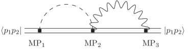
The action (3) allows for a wide variety of triple multipole diagrams. The lowest contributing terms are those containing two electric quadrupole moments, because $E$ and $L_{k}$ are conserved in the stationary case we are considering. The diagram QEQ is of $O(v^{10})$ or of lowest order 4PN. The diagrams QLQ, JEJ, OEO and QQQ are of $O(v^{12})$ and of lowest order 5PN. Other valid combinations are of higher than 5PN order or vanish, except the QQQ combination with two gravitons and one two–graviton $Q_{ij}$ interaction.

In the following we list the local finite 5PN contributions from the electric quadrupole moment, $H_{\rm el.quad}^{\rm 5PN}$, the octupole term, $H_{\rm oct.}$, the magnetic quadrupole moment, $H_{\rm mag.quad.}$, the angular momentum term $H_{\rm ang.}$, and the three contributions to the memory term, $H_{\rm mem.1,2,3}$, expressed in terms of the rescaled orbital distance $r=r_{\text{phys}}c^{2}/(G_{N}M)$.

$$H_{\rm el.quad}^{\rm 5PN} = \nu\Biggl{[}-(1-3\nu)\frac{1}{r^{3}}\Biggl{(}\frac{392}{75}p^{6}-\frac{3508}{75}p^{4}(p.n)^{2}+\frac{124}{3}p^{2}(p.n)^{4}\Biggr{)}$$ (12)

$$+\frac{1}{r^{4}}\Biggl{(}-\frac{2(4573+32831\nu)p^{4}}{3675}-\frac{2(-598985+122233\nu)p^{2}(p.n)^{2}}{3675}$$

$$+\frac{4(-286508+54209\nu)(p.n)^{4}}{3675}\Biggr{)}+\frac{1}{r^{5}}\Biggl{(}\Biggl{(}\frac{696}{1225}+\frac{77428\nu}{3675}\Biggr{)}p^{2}$$

$$+\Biggl{(}\frac{30904}{3675}+\frac{19168\nu}{735}\Biggr{)}(p.n)^{2}\Biggr{)}+\frac{8(-244+137\nu)}{525r^{6}}\Biggr{]},$$

$$H_{\rm oct.} = (1-4\nu)\nu\Biggl{[}\frac{1}{r^{4}}\Biggl{(}\frac{17657p^{4}}{2205}-\frac{130058p^{2}(p.n)^{2}}{3675}+\frac{60409(p.n)^{4}}{2205}\Biggr{)}$$ (13)

$$+\frac{1}{r^{5}}\Biggl{(}-\frac{2848p^{2}}{1575}+\frac{20848(p.n)^{2}}{11025}\Biggr{)}+\frac{4}{7r^{6}}\Biggr{]},$$

$$H_{\rm mag.quad.} = (1-4\nu)\nu\Biggl{[}\frac{1}{r^{4}}\Biggl{(}\frac{58p^{4}}{45}-\frac{604p^{2}(p.n)^{2}}{75}+\frac{1522(p.n)^{4}}{225}\Biggr{)}-\frac{1}{r^{5}}\frac{488}{225}(p^{2}-(p.n)^{2})\Biggr{]},$$

$$H_{\rm ang.} = \nu^{2}\Biggl{[}\frac{1}{r^{4}}\Biggl{(}-\frac{256p^{4}}{5}+\frac{1056p^{2}(p.n)^{2}}{5}-160(p.n)^{4}\Biggr{)}+\frac{1}{r^{5}}\frac{256}{15}(p^{2}-(p.n)^{2})\Biggr{]}.$$ (15)

Note that the terms $\propto\ln(r/r_{0})$ occurring have been considered together with the non–local terms here.

For all these terms we agree with the principle structure given in Ref. [30], where the multipole moments were not inserted, with the exception that $H_{\rm mag.quad.}$ still needs the finite renormalization as described in Ref. [13], which here has already been considered. In the same way we agree with the 4PN tail term ${\sf QEQ}$.

In the EFT calculation the choice of the time dependence of the propagators in these 5PN cases turns out to be irrelevant in the explicit calculation, since the causal and the in–in formalism lead to the same result. The reason for this is that the internal multipole moment, either $E$ or $L^{k}$, is a conserved quantity, implying a $\delta$–distribution for the energy components at their vertex. The associated propagator is therefore an (effective) space–like potential and the corresponding diagram only depends on a single energy variable, $k_{0}$. In the case of the potential terms, cf. [9, 11], the reason for the same agreement is different. Here the propagators in Fourier–space are expanded as

$$\frac{1}{\vec{k}^{2}-k_{0}^{2}\pm i\varepsilon}=\frac{1}{\vec{k}^{2}}\sum_{l=0}^{\infty}\left(\frac{k_{0}^{2}}{\vec{k}^{2}}\right)^{l},$$ (16)

in which the $i\varepsilon$–prescription does not play a role. When the in–in formalism is used for all these terms, it leads to the same results as using the usual (causal) path integral [63, 64].

Indeed, a fundamental argument has been raised for the general use of the in–in formalism by B. DeWitt [59]. In using $S$–matrix theory the LSZ–formalism [65] requires a clear definition of the Hilbert spaces both for the initial state at $t=-\infty$ and for the final state at $t=+\infty$, made of (interaction) free states in both cases. This is fulfilled in elementary particle scattering processes, however, not in inspiraling processes like the merging of two large masses. While the initial state can be very well defined as

$$|p_{1}p_{2}\rangle=|p_{1}\rangle|p_{2}\rangle,$$ (17)

with $p_{1}$ and $p_{2}$ the 4–momenta of the non–interacting masses at $t=-\infty$, the synonymous information on the final state of the merging process at $t=+\infty$ is not really known. The in–in formalism, however, requires only to know the initial state.

The contributions to the far-zone term require retarded boundary conditions, as known from the Feynman–Wheeler formalism [69, 70] in Quantum Electrodynamics. The Schwinger formalism using in–in states provides this description. As well–known, both the usual path–integral formalism [63, 64], leading to causal Green’s functions with $T^{*}$–ordering, and, analogously, the so-called in–in formalism, cf. [50, 61], are exactly defined, also concerning the type of the contributing propagators. The in–in formalism has also applications in statistical physics, cf. [52, 55]. A critical question concerns the unitarity of the respective formalism. As has been shown in [57] this is obeyed for the in–in formalism at least at two–loop order, the level necessary at 5PN. In the EFT approach the far-zone diagrams up 5PN read structurally as shown in Figure 1 using the in–in formalism: these are diagrams containing three multipole moments with single or double graviton interaction between two in–states. Also here the gravitons have at most self–couplings and all end at the worldline being connected to one of the multipole moment insertions.

The only contributing diagrams at 5PN are two–loop diagrams. In the action, the 2–loop graviton exchange is integrated out. The necessary Feynman rules are listed in Appendix A. One then may read off the contributions to the conservative far-zone Lagrangian (Hamiltonian) from the action directly. The in–in formalism is described in detail in Appendix C.

In the following we calculate the contributions to the memory term in the in–in formalism. This differs from the previous work [30], which employed a variant of the in–out formalism with Feynman Green’s functions replaced by advanced or retarded ones. Further differences may arise in the Feynman rules, which are not stated explicitly in [30]. The $D$ dimensional tensor integrals are decomposed using the Passarino–Veltman representation [71] and the momentum integrals are performed using hypergeometric techniques [72, 73] after a Feynman parameterization. In the final result the $\varepsilon$ dependence cancels, as the case of $H_{\rm ang.}$, leaving the integrals over the energy components.

The results for the diagrams in Figure 1 are

$$H_{\rm mem.1} = \nu^{2}\Biggl{[}\frac{1}{r^{4}}\Biggl{(}{-}\frac{10p^{4}}{3}{+}\frac{967p^{2}(p.n)^{2}}{54}{-}\frac{83(p.n)^{4}}{6}\Biggr{)}+\frac{1}{r^{5}}\Biggl{(}{+}\frac{77p^{2}}{27}{-}\frac{97(p.n)^{2}}{27}\Biggr{)}{-}\frac{11}{27r^{6}}\Biggr{]}$$

for the term in the l.h.s. and we obtain for the two contributions of the second diagram

$$H_{\rm mem.2} = \nu^{2}\Biggl{[}\frac{1}{r^{4}}\Biggl{(}4p^{4}{-}\frac{967p^{2}(p.n)^{2}}{45}{+}\frac{83(p.n)^{4}}{5}\Biggr{)}+\frac{1}{r^{5}}\Biggl{(}{-}\frac{154p^{2}}{45}{+}\frac{194(p.n)^{2}}{45}\Biggr{)}{+}\frac{22}{45r^{6}}\Biggr{]},$$

$$H_{\rm mem.3} = \nu^{2}\Biggl{[}\frac{1}{r^{4}}\Biggl{(}\frac{16p^{4}}{315}{+}\frac{152p^{2}(p.n)^{2}}{105}{-}\frac{8(p.n)^{4}}{7}\Biggr{)}+\frac{1}{r^{5}}\Biggl{(}{-}\frac{16p^{2}}{105}{+}\frac{256(p.n)^{2}}{315}\Biggr{)}{+}\frac{32}{315r^{6}}\Biggr{]}.$$

Details of the calculation of the $H_{\rm mem.}$ terms are given in Appendix D. The results in (2–2) differ from those given in [30] by a factor and the calculation of the contribution (2) is new. We have repeated the calculation of (2–2) in the same manner as described in [30] and agree. However, our result is based on the derivation of the corresponding graph using the path integral in the in–in formalism and differs from that in [30]. There a specific choice for linking the advanced and retarded propagators has been made, which is not confirmed.

We also would like to mention that we have slightly modified the Hamiltonian given in [13], by treating higher time derivatives in the action, which are now eliminated by partial integration. This change, however, just corresponds to a canonical transformation, as we will show below in calculating observables which come out the same. The complete local pole–free Hamiltonian, with tags on different contributions, is given in computer readable form in the ancillary file HAMILTONIAN.m to this paper.

3 Determining the EOB potentials from the Hamiltonian in harmonic coordinates

In Ref. [16] we have calculated the 5PN potential contributions to the Hamiltonian using dimensional regularization in $D=4-2\varepsilon$ space–time dimensions, including the pole terms and the non–local far-zone contribution in complete form using harmonic coordinates. The sum of these terms does still contain a pole contribution $1/\varepsilon$. A canonical transformation leads to a pole–free Hamiltonian. In [16] we have left out finite rational 5PN terms of $O(\nu^{2})$, i.e. local far-zone contributions which are purely rational. We have presented already all the $\pi^{2}$ terms of $O(\nu^{2})$ since they stem from the potential terms.

A central point of our investigation is to compare to previous results given in Ref. [15], which have been presented based on a 5PN EOB Hamiltonian. For the local parts of both Hamiltonians one may either perform a canonical transformation, as done in Ref. [16], or determine the EOB potentials by an observable. We will choose the latter way and use the local contribution to periastron advance $K^{\rm loc,h}(\hat{E},j)$. Corresponding consistency checks can be performed by additional observables, such as the binding energy and periastron advance for circular motion and also the expansion coefficients of the scattering angle.

3.1 The EOB parameters

The EOB Hamiltonian is given by [15]

$$H_{\rm EOB}^{\rm loc,eff}=\sqrt{A(1+AD\eta^{2}(p.n)^{2}+\eta^{2}(p^{2}-(p.n)^{2})+Q)},$$ (21)

which we consider up to the contributions to 5PN. Here $\eta=1/c$ denotes the post–Newtonian expansion parameter, with $c$ the velocity of light. The potentials $A,D$ and $Q$ are parameterized by

$$A = 1+\sum_{k=1}^{6}a_{k}(\nu)\eta^{2k}u^{k},\leavevmode\nobreak\ \leavevmode\nobreak\ a_{2}=0,$$ (22)

$$D = 1+\sum_{k=2}^{5}d_{k}(\nu)\eta^{2k}u^{k},$$ (23)

$$Q = \eta^{4}(p.n)^{4}[q_{42}(\nu)\eta^{4}u^{2}+q_{43}(\nu)\eta^{6}u^{3}+q_{44}(\nu)\eta^{8}u^{4}]+\eta^{6}(p.n)^{6}[q_{62}(\nu)\eta^{4}u^{2}+q_{63}(\nu)\eta^{6}u^{3}]$$ (24)

$$+\eta^{12}(p.n)^{8}u^{2}q_{82}(\nu),$$

where $u=1/r$.

The known 4PN Hamiltonians [7, 8, 9, 10, 11] in harmonic and ADM coordinates are connected by canonical transformations to $H_{\rm EOB}$, cf. [11],which imply the expansion parameters

$${\rm N},u\leavevmode\nobreak\ : \leavevmode\nobreak\ a_{1} = \leavevmode\nobreak\ -2,$$ (25)

$${\rm 2PN},u^{2}: \leavevmode\nobreak\ d_{2} = \leavevmode\nobreak\ 6\nu,$$ (26)

$$u^{3}: \leavevmode\nobreak\ a_{3} = \leavevmode\nobreak\ 2\nu,$$ (27)

$${\rm 3PN},u^{2}: \leavevmode\nobreak\ q_{42} = \leavevmode\nobreak\ 8\nu-6\nu^{2},$$ (28)

$$u^{3}: \leavevmode\nobreak\ d_{3} = \leavevmode\nobreak\ 52\nu-6\nu^{2},$$ (29)

$$u^{4}: \leavevmode\nobreak\ a_{4} = \leavevmode\nobreak\ \left(\frac{94}{3}-\frac{41}{32}\pi^{2}\right)\nu,$$ (30)

$${\rm 4PN},u^{2}: \leavevmode\nobreak\ q_{62} = \leavevmode\nobreak\ -\frac{9}{5}\nu-\frac{27}{5}\nu^{2}+6\nu^{3},$$ (31)

$$u^{3}: \leavevmode\nobreak\ q_{43} = \leavevmode\nobreak\ 20\nu-83\nu^{2}+10\nu^{3},$$ (32)

$$u^{4}: \leavevmode\nobreak\ d_{4} = \leavevmode\nobreak\ \left(\frac{1679}{9}-\frac{23761}{1536}\pi^{2}\right)\nu+\left(-260+123\pi^{2}\right)\nu^{2},$$ (33)

$$u^{5}: \leavevmode\nobreak\ a_{5} = \leavevmode\nobreak\ \left(-\frac{4237}{60}+\frac{2275}{512}\pi^{2}\right)\nu+\left(-\frac{221}{6}+\frac{41}{32}\pi^{2}\right)\nu^{2}.$$ (34)

The expansion coefficients $a_{6},\bar{d}_{5},q_{44},q_{63}$ and $q_{82}$ emerge at 5PN. In [15] the following values were obtained

$${\rm 5PN},u^{2}\leavevmode\nobreak\ : \leavevmode\nobreak\ q_{82} = \leavevmode\nobreak\ \frac{6}{7}\nu+\frac{18}{7}\nu^{2}+\frac{24}{7}\nu^{3}-6\nu^{4},$$ (35)

$$u^{3}\leavevmode\nobreak\ : \leavevmode\nobreak\ q_{63} = \leavevmode\nobreak\ \frac{123}{10}\nu-\frac{69}{5}\nu^{2}+116\nu^{3}-14\nu^{4},$$ (36)

$$u^{4}\leavevmode\nobreak\ : \leavevmode\nobreak\ q_{44} = \leavevmode\nobreak\ \left(\frac{1580641}{3150}-\frac{93031}{1536}\pi^{2}\right)\nu+\left(-\frac{9367}{15}+\frac{31633}{512}\pi^{2}\right)\nu^{2}+\left(640-\frac{615}{32}\pi^{2}\right)\nu^{3},$$ (37)

$$u^{5}: \leavevmode\nobreak\ \bar{d}_{5} = \leavevmode\nobreak\ \left(\frac{331054}{175}-\frac{63707}{512}\pi^{2}\right)\nu+\bar{d}_{5}^{\nu^{2}}\nu^{2}+\left(\frac{1069}{3}-\frac{205}{16}\pi^{2}\right)\nu^{3},$$ (38)

$$u^{6}: \leavevmode\nobreak\ a_{6} = \leavevmode\nobreak\ \left(-\frac{1026301}{1575}+\frac{246367}{3072}\pi^{2}\right)\nu+a_{6}^{\nu^{2}}\nu^{2}+4\nu^{3}.$$ (39)

In Ref. [13] we have calculated the $\pi^{2}$ contributions to $\bar{d}_{5}^{\nu^{2}}$ and $a_{6}^{\nu^{2}}$ which read

$$\bar{d}_{5}^{\pi^{2}\nu^{2}} = \frac{306545}{512}\pi^{2}\nu^{2},$$ (40)

$$a_{6}^{\pi^{2}\nu^{2}} = \frac{25911}{256}\pi^{2}\nu^{2}.$$ (41)

All 5PN coefficients can be obtained from the periastron advance $K^{\rm loc,h}(\hat{E},j)$, expressed in terms of the energy $\hat{E}$ obtained from the reduced Hamiltonian,

$${\hat{H}=\frac{H-Mc^{2}}{\mu c^{2}}},$$ (42)

and the rescaled angular momentum defined in eq. (53). Explicit formulas for the calculation of $K^{\rm loc,h}(\hat{E},j)$ from a Hamiltonian are given e.g. in [16]. Comparing the results obtained from the Hamiltonian (2) in harmonic coordinates and the EOB Hamiltonian (21) one finds

$$q_{82} = \frac{6}{7}\nu+\frac{18}{7}\nu^{2}+\frac{24}{7}\nu^{3}-6\nu^{4},$$ (43)

$$q_{63} = \frac{123}{10}\nu-\frac{69}{5}\nu^{2}+116\nu^{3}-14\nu^{4},$$ (44)

$$q_{44} = \left(\frac{1580641}{3150}-\frac{93031\pi^{2}}{1536}\right)\nu+\left({-\frac{3670222}{4725}}+\frac{31633\pi^{2}}{512}\right)\nu^{2}+\left(640-\frac{615}{32}\pi^{2}\right)\nu^{3},$$ (45)

$$\bar{d}_{5} = \left(\frac{331054}{175}-\frac{63707}{512}\pi^{2}\right)\nu+\left({-\frac{31295104}{4725}}+\frac{306545}{512}\pi^{2}\right)\nu^{2}+\left(\frac{1069}{3}-\frac{205}{16}\pi^{2}\right)\nu^{3},$$

$$a_{6} = \left(-\frac{1026301}{1575}+\frac{246367}{3072}\pi^{2}\right)\nu+\left({-\frac{1749043}{1575}}+\frac{25911}{256}\pi^{2}\right)\nu^{2}+4\nu^{3}.$$ (47)

Here $q_{82}$ is uniquely determined by comparing the respective coefficients of $\hat{E}^{4}/j^{2}$, whereas $q_{63}$ and $q_{44}$ follow from the $\hat{E}^{3}/j^{4}$ term, etc. Values for $\bar{d}_{5}$ and $a_{6}$, which are consistent with (3.1) and (47), are also obtained from the binding energy and periastron advance in the circular case, which do not depend on the $Q$–potentials.

3.2 The scattering angle

We will now study the expansion coefficients $\chi_{k}$ of the scattering angle starting with its local contributions. We use the well known relations

$$\frac{\chi^{\rm loc}+\pi}{2}=\sum_{k=1}^{\infty}\frac{\chi_{k}^{\rm loc}}{j^{k}}={\sf Reg}_{u_{\rm max}}\int_{\varepsilon}^{u_{\rm max}(\varepsilon)}\frac{jdy}{(p.n)(y,j)},\leavevmode\nobreak\ \leavevmode\nobreak\ p.n\leavevmode\nobreak\ :=\leavevmode\nobreak\ \sqrt{p_{\infty}^{2}-j^{2}y^{2}+W(y,p_{\infty})},$$ (48)

with $u_{\rm max}(\varepsilon)=(1+\sqrt{1+j^{2}p_{\infty}^{2}})/(jp_{\infty})-\varepsilon$, cf. also [23], Eq. (3.39). One also has

$$\frac{\chi^{\rm loc}}{2}={\sf Reg}_{\varepsilon}\sum_{n=1}^{\infty}\int_{\varepsilon}^{1-\varepsilon}dx\binom{-\tfrac{1}{2}}{n}(1-x^{2})^{-\frac{1}{2}-n}\left[\tilde{w}\left(\frac{x}{j}\right)\right]^{n},$$ (49)

with

$$\tilde{w}=\sum_{k=1}^{\infty}w_{k}\frac{x^{k}}{j^{k}}.$$ (50)

Here the operator ${\sf Reg}_{\varepsilon}$ drops the singular terms in $\varepsilon$ in the limit $\varepsilon\rightarrow 0$.

Some of the integrals are listed in Appendix E. Here the following kinematic variables are used, cf. [20, 75],

$$p_{\infty}\leavevmode\nobreak\ = \leavevmode\nobreak\ \sqrt{\gamma^{2}-1},$$ (51)

$$\gamma\leavevmode\nobreak\ = \leavevmode\nobreak\ \frac{1}{m_{1}m_{2}}[E_{1}E_{2}+p^{2}],\leavevmode\nobreak\ \leavevmode\nobreak\ \leavevmode\nobreak\ E_{i}=\sqrt{p^{2}+m_{i}^{2}},$$ (52)

$$j\leavevmode\nobreak\ = \leavevmode\nobreak\ \frac{J}{G_{N}m_{1}m_{2}},$$ (53)

$$\Gamma\leavevmode\nobreak\ = \leavevmode\nobreak\ \sqrt{1+2\nu(\gamma-1)},$$ (54)

$E_{i}$ are the corresponding energies, $p$ the cms momentum, and $J$ the angular momentum. Note that in the definition of the scattering angle in Ref. [15], Eq. (9.1), the regularization operator has not been written, although being necessary, cf. e.g. Eq. (3.49) in [23] (in the energy gauge), since both the expansion in $1/j$ and the post–Newtonian expansion is finally carried out.

The quantity $q_{63}$ can be extracted from the component $\chi_{3}^{\rm h,loc}$ of the scattering angle from the contribution $O(p_{\infty}^{7})$

$$\chi_{3}^{\rm h,loc} = -\frac{1}{3p_{\infty}^{3}}+\frac{4\eta^{2}}{p_{\infty}}+\eta^{4}(24-8\nu)p_{\infty}+\eta^{6}\left(\frac{64}{3}-36\nu+8\nu^{2}\right)p_{\infty}^{3}+\eta^{8}\left(-\frac{91}{5}\nu+34\nu^{2}\right.$$ (55)

$$\left.-8\nu^{3}\right)p_{\infty}^{5}+\eta^{10}\left(\frac{96}{35}\nu+\frac{288}{35}\nu^{2}-\frac{108}{7}\nu^{3}+6\nu^{4}-\frac{1}{7}q_{63}\right)p_{\infty}^{7}.$$

From

$$\chi_{3}^{\rm h,loc} = \chi_{3}^{\rm Schw}-\frac{2\nu p_{\infty}}{\Gamma^{2}}\left[\frac{2}{3}\gamma(14\gamma^{2}+25)+\frac{4(4\gamma^{4}-12\gamma^{2}-3)}{p_{\infty}}{\rm arcsinh}\left(\sqrt{\frac{\gamma-1}{2}}\right)\right]$$ (56)

$$= -\frac{1}{3p_{\infty}^{3}}+\frac{4\eta^{2}}{p_{\infty}}+(24-8\nu)\eta^{3}p_{\infty}+\left(\frac{64}{3}-36\nu+8\nu^{2}\right)\eta^{6}p_{\infty}^{3}+\left(-\frac{91}{5}\nu+34\nu^{2}-8\nu^{3}\right)$$

$$\times\eta^{8}p_{\infty}^{5}+\left(\frac{69}{70}\nu+\frac{51}{5}\nu^{2}-32\nu^{3}+8\nu^{4}\right)\eta^{10}p_{\infty}^{7}$$

and (LABEL:eq:chi31) one obtains $q_{63}$ as in Eq. (44).

In Eq. (48) $(p.n)$ is calculated as in the case for periastron advance [13] and by setting

$$\hat{E}=\frac{\Gamma-1}{\nu}$$ (57)

and expanding to the respective post–Newtonian order. The operator ${\sf Reg}_{u_{\rm max}}$ removes all pole terms in $\varepsilon$, which are implied in the integral (48) by

$$y=u_{\rm max}:=\frac{1}{jp_{\infty}}\left[1+\sqrt{1+j^{2}p_{\infty}^{2}}\right]-\varepsilon,$$ (58)

where we choose $|\varepsilon|\ll 1$. In using (48) for the calculation of $\chi_{k}^{\rm loc}$, singular terms in $\varepsilon$ in the corresponding integrals are disregarded. Here the expansion coefficients of the Schwarzschild scattering angle $\chi_{k}^{\rm Schw}$ are given by

$$\frac{\chi^{\rm Schw}}{2}=\sum_{k=1}^{\infty}\frac{1}{j^{k}}\chi_{k}^{\rm Schw},$$ (59)

with

$$\chi^{\rm Schw}_{k} ={\sf Reg}_{\varepsilon}\binom{-\tfrac{1}{2}}{k}\eta^{k}\int_{0}^{\sqrt{\eta^{2}p_{\infty}^{2}-\varepsilon}}dy\frac{[2y(1+y^{2})]^{k}}{(p_{\infty}^{2}\eta^{2}-y^{2})^{k+1/2}}, \leavevmode\nobreak\ {k\leavevmode\nobreak\ \leavevmode\nobreak\ \rm even}$$

$$=\frac{(-1)^{k+1}2^{k-1}}{p_{\infty}^{k}}\binom{-\tfrac{1}{2}}{k}\frac{\Gamma(\tfrac{k+1}{2})\Gamma(\tfrac{1}{2}-k)}{\Gamma(1-\tfrac{k}{2})}{}_{2}F_{1}\biggl{[}\genfrac{.}{.}{0.0pt}{}{-k\mskip 8.0mu\tfrac{k+1}{2}}{1-\tfrac{k}{2}};-\eta^{2}p^{2}_{\infty}\biggr{]}, \leavevmode\nobreak\ {k\leavevmode\nobreak\ \leavevmode\nobreak\ \rm odd}.$$ (60)

${\sf Reg}_{\varepsilon}$ projects onto the constant part in the $\varepsilon$-expansion, which correspondingly implies a regularization scheme dependence. However, the relation

$$\chi_{2k}^{\rm h,loc}(p_{\infty},\nu)=\frac{\pi}{2}K^{\rm loc,h}_{2k}(\hat{E}),$$ (61)

with

$$K^{\rm loc,h}(\hat{E},j)=\sum_{k=1}^{\infty}\frac{1}{j^{2k}}K^{\rm loc,h}_{2k}(\hat{E}),$$ (62)

cf. [22], can be used in the limit $\nu\rightarrow 0$, fixing the regularization scheme. In Eq. (61) it is understood, that $\hat{E}$ of (57) is used and an expansion in $p_{\infty}$ to the respective PN order is performed. In the present case we use the choice (3.2). We label the different post–Newtonian contributions by the parameter $\eta$. For the first orders in the expansion of (59) one obtains

$$\chi^{\rm Schw}_{1} = \frac{1}{p_{\infty}}+2p_{\infty}\eta^{2},$$ (63)

$$\chi^{\rm Schw}_{2} = \pi\left(\frac{3}{2}\eta^{2}+\frac{15}{8}p_{\infty}^{2}\eta^{4}\right),$$ (64)

$$\chi^{\rm Schw}_{3} = -\frac{1}{3p_{\infty}^{3}}+\frac{4\eta^{2}}{p_{\infty}}+24p_{\infty}\eta^{4}+\frac{64}{3}p_{\infty}^{3}\eta^{6},$$ (65)

$$\chi^{\rm Schw}_{4} = \pi\left(\frac{105}{8}\eta^{4}+\frac{315}{8}p_{\infty}^{2}\eta^{6}+\frac{3465}{128}p_{\infty}^{4}\eta^{8}\right).$$ (66)

Higher–order expansion coefficients are listed in Appendix E. The coefficients $q_{82}$ and $q_{44}$ can also be extracted from the component $\chi_{2}^{\rm h}$ and $\chi_{4}^{\rm h}$ of the scattering angle, respectively, using relation (61) by expanding to $O(p_{\infty}^{6})$. One obtains the values given in Eqs. (43, 45). For $q_{44}$ we observe the difference

$$q_{44}-q_{44}^{\rm Ref.\text{\cite[cite]{[\@@bibref{}{Bini:2020wpo}{}{}]}}}={-\frac{719617}{4725}\nu^{2}}.$$ (67)

This coefficient is related to the $\hat{E}^{3}/j^{4}$ term of the periastron advance $K^{\rm loc,h}(\hat{E},j)$. The potential contributions to this quantity are of $O(G_{N}^{4})$ and have been first obtained in [16]. They have recently been confirmed by the $O(G_{N}^{4})$ post–Minkowskian results of [76], cf. also [77, 78]. The $O(\nu^{2}\pi^{2})$ contribution to this term is implied by $q_{44}$, since $q_{82}$ and $q_{63}$ are purely rational in $\nu$. We also would like to mention that the $\pi^{2}$ terms of $\bar{d}_{5}$ and $a_{6}$, as determined using the scattering angle in [42], using the potential terms given in [16], are equivalently obtained by using Eqs. (61, 62), which has been presented before in Ref. [16].

The above expansion coefficients at 5PN were all derived without referring to a specific $\nu$ dependence of the combination [23]

$$\Gamma^{k-1}\chi_{k}-\chi_{k}^{\rm Schw}.$$ (68)

The equations determining the rational $O(\nu^{2})$ terms of $q_{44},\bar{d}_{5}$ and $a_{6}$ contain also local far-zone contributions, which are finite and just of $O(\nu^{2})$ together with the $O(\nu^{2})$ from singular far-zone terms, which are fully predicted in relation to their $O(\nu)$ contributions, cf. [16]. This aspect will be also discussed in Section 4.

From the results obtained in the previous sections we determine now the $O(\nu^{2})$ contributions to $q_{44},a_{6}$ and $\bar{d}_{5}$. We first consider $\chi_{4}^{\rm total,h}$,

$$\chi_{4}^{\rm total,h}=\chi_{4}^{\rm nonloc,h}+\chi_{4}^{\rm loc,h}.$$ (69)

The non–local contribution, $\chi_{4}^{\rm nonloc,h}$, has been calculated in [15] and is given by

$$\chi_{4}^{\rm nonloc,h} = \nu\eta^{8}p_{\infty}^{4}\pi\Biggl{\{}-\frac{63}{4}-\eta^{2}\left(\frac{2753}{1120}-\frac{1071}{40}\nu\right)p_{\infty}^{2}-\ln\left(\frac{p_{\infty}}{2}\right)\Biggl{[}\frac{37}{5}+\eta^{2}\left(\frac{1357}{280}-\frac{111}{10}\nu\right)p_{\infty}^{2}\Biggr{]}\Biggr{\}}$$

Its transform to the f–scheme for $\Gamma^{3}\chi_{4}^{\rm f-h}$ is given in Eq. (8.6) there, to eliminate the term of $O(\pi\nu^{2}p_{\infty}^{6})$. One has

$$\Gamma^{3}\chi_{4}^{\rm nonloc,h} = \nu\eta^{8}p_{\infty}^{4}\pi\Biggl{\{}-\frac{63}{4}-\frac{37}{5}\ln\left(\frac{p_{\infty}}{2}\right)+\eta^{2}p_{\infty}^{2}\Biggl{[}-\frac{2753}{1120}-\frac{1357}{280}\ln\left(\frac{p_{\infty}}{2}\right)+\frac{63}{20}\nu\Biggr{]}\Biggr{\}}.$$ (71)

The local contribution is obtained from Eq. (61) including all local contributions to the Hamiltonian, and reads

$$\chi_{4}^{\rm loc,h} = \pi\Biggl{\{}\eta^{4}\Biggl{(}\frac{105}{8}-\frac{15}{4}\nu\Biggr{)}+\eta^{6}\Biggl{[}\frac{315}{8}-\Biggl{(}\frac{109}{2}-\frac{123}{256}\pi^{2}\Biggr{)}\nu+\frac{45}{8}\nu^{2}\Biggr{]}p_{\infty}^{2}$$ (72)

$$+\eta^{8}\Biggl{[}\frac{3465}{128}-\Biggl{(}\frac{19597}{192}-\frac{33601}{16384}\pi^{2}\Biggr{)}\nu+\Biggl{(}\frac{4827}{64}-\frac{369}{512}\pi^{2}\Biggr{)}\nu^{2}-\frac{225}{32}\nu^{3}\Biggr{]}p_{\infty}^{4}$$

$$+\eta^{10}\Biggl{[}-\Biggl{(}\frac{1945583}{33600}-\frac{93031}{32768}\pi^{2}\Biggr{)}\nu+\Biggl{(}{\frac{12605197}{100800}}-\frac{94899}{32768}\pi^{2}\Biggr{)}\nu^{2}$$

$$-\Biggl{(}\frac{2895}{32}-\frac{1845}{2048}\pi^{2}\Biggr{)}\nu^{3}+\frac{525}{64}\nu^{4}\Biggr{]}p_{\infty}^{6}\Biggr{\}},$$

and one obtains

$$\Gamma^{3}\chi_{4}^{\rm loc,h}-\chi_{4}^{\rm Schw} = \pi\nu\Biggl{[}-\frac{15}{4}\eta^{4}+\eta^{6}p_{\infty}^{2}\left(-\frac{557}{16}+\frac{123}{256}\pi^{2}\right)+\eta^{8}p_{\infty}^{4}\left(-\frac{4601}{96}+\frac{33601}{16384}\pi^{2}\right)$$ (73)

$$+\eta^{10}p_{\infty}^{6}\left(-\frac{3978707}{134400}+\frac{93031}{32768}\pi^{2}+{\frac{402097}{100800}}\nu\right)\Biggr{]}.$$

Forming the combination (68) and expanding to $O(\eta^{10})$ (5PN) we obtain

$$\left[\Gamma^{3}\chi_{4}^{\rm total,h}-\chi_{4}^{\rm Schw}\right]-\left[\Gamma^{3}\chi_{4}^{\rm total,h}-\chi_{4}^{\rm Schw}\right]^{\text{\rm Ref.\leavevmode\nobreak\ \cite[cite]{[\@@bibref{}{Bini:2020wpo}{}{}]}}}={\frac{719617}{100800}}\eta^{10}\pi\nu^{2}p_{\infty}^{6},$$ (74)

comparing with the result of Ref. [15], Eqs. (8.2, 8.6, 10.1c, 10.2d), and thus observe a breaking of the rule

$$\left[\Gamma^{k-1}\chi_{k}^{\rm total,h}-\chi_{k}^{\rm Schw}\right]=P_{k}(\nu)$$ (75)

with degree of $[(k-1)/2]$ of the polynomial $P_{k}(\nu)$.

On the other hand, one observes for $k\in[1,3]$, that (75) holds. It is trivially obeyed for $k=1,2$ because of the post–Minkowskian structure [79], see also [23], and is implied for $k=3$ by

$$\Gamma^{3}{\chi}^{\rm h,loc}_{3}-\chi_{3}^{\rm Schw}\leavevmode\nobreak\ = \leavevmode\nobreak\ \nu\left[-\frac{\eta^{2}}{3p_{\infty}}-\frac{47}{12}\eta^{4}p_{\infty}-\frac{313}{24}\eta^{6}p_{\infty}^{3}-\frac{749}{320}\eta^{8}p_{\infty}^{5}-\frac{7519}{4480}\eta^{10}p_{\infty}^{7}\right]+O(p_{\infty}^{9}),$$

referring to the $O(G_{N}^{3})$ post–Minkowskian Hamiltonian [24]. Note that for $k\leq 3$ no far-zone terms contribute and the scattering angle stems from the potential contributions only. The post–Minkowskian result of $O(G_{N}^{3})$ [24] has been checked to 6PN in [20].

Finally we would like to discuss the hypothetical possibility to accommodate the result of the present paper on $q_{44}$ with the one in [15]. In a later paper, [42], the authors of [15] claim to have still a missing term in Eq. (10.2) of [42] on radiation reaction, which is not yet quantified. It is of the type

$$\delta H_{\text{{rad}}}=a\eta^{10}\nu^{2}\frac{(p.n)^{4}}{r^{4}},$$ (77)

with $a\in\mathbb{R}$. We stress that to the best of our knowledge no such contributions are missing in the present EFT approach. Terms of the kind (77) can imply the mapping

$$q_{44}^{\rm h}\rightarrow q_{44}^{\text{\rm Ref.\leavevmode\nobreak\ \cite[cite]{[\@@bibref{}{Bini:2020wpo}{}{}]}}}$$ (78)

here with the value

$$a={\frac{402097}{9450}},$$ (79)

to reach full agreement. It transforms $K(\hat{E},j)^{\rm 5PN}_{\rm loch}$ into [19], Eq. (F.5). This also applies e.g. to $\chi_{k}^{\rm loc},\leavevmode\nobreak\ k=4,5,6$, while $E^{\rm circ}$ and $K^{\rm circ}$ remain unaffected, see Section 4. We finally note that in the post–Minkowskian apprach $\chi_{k}(j)$ is derived from the terms of $O(G_{N}^{k})$ and are presently known for all contributions to $k=4$.

4 Phenomenological results

In the following we summarize the results of the present calculation for observables and present numerical results. We illustrate the result for the local 5PN contribution to the local contributions to general periastron advance $K^{\rm loc,h}(\hat{E},j)$ and the circular limits of the binding energy $E^{\rm circ}(j)$ and periastron advance $K^{\rm circ}(j)$ which are given by

$$K(\hat{E},j)_{\rm loc,h}^{\rm 5PN} = \Biggl{\{}\Biggl{[}\frac{15\nu^{2}}{16}-\frac{15}{4}\nu^{3}+3\nu^{4}\Biggr{]}\frac{\hat{E}^{4}}{j^{2}}+\Biggl{[}\frac{3465}{16}+\left(-\frac{12160657}{8400}+\frac{15829\pi^{2}}{256}\right)\nu+\Biggl{(}{\frac{10575547}{6300}}$$ (80)

$$-\frac{35569\pi^{2}}{1024}\Biggr{)}\nu^{2}+\Biggl{(}\frac{1107\pi^{2}}{128}-\frac{7113}{8}\Biggr{)}\nu^{3}+75\nu^{4}\Biggr{]}\frac{\hat{E}^{3}}{j^{4}}+\Biggl{[}\frac{315315}{32}+\Biggl{(}-\frac{33023719}{840}$$

$$+\frac{4899565\pi^{2}}{4096}\Biggr{)}\nu+\Biggl{(}-\frac{3289285\pi^{2}}{1024}+{\frac{139190707}{2520}}\Biggr{)}\nu^{2}+\Biggl{(}\frac{35055\pi^{2}}{256}-\frac{240585}{32}\Biggr{)}\nu^{3}$$

$$+\frac{1575}{8}\nu^{4}{\Biggr{]}}\frac{\hat{E}^{2}}{j^{6}}+\Biggl{[}\frac{765765}{16}+\Biggl{(}-\frac{30690127}{240}+\frac{16173395\pi^{2}}{8192}\Biggr{)}\nu+\Biggl{(}{\frac{67444909}{432}}$$

$$-\frac{77646205\pi^{2}}{8192}\Biggr{)}\nu^{2}+\Biggl{(}\frac{121975\pi^{2}}{512}-\frac{271705}{24}\Biggr{)}\nu^{3}+\frac{2205}{16}\nu^{4}\Biggr{]}\frac{\hat{E}}{j^{8}}+\Biggl{[}\frac{2909907}{64}$$

$$+\Biggl{(}-\frac{61358067}{640}+\frac{1096263\pi^{2}}{1024}\Biggr{)}\nu+\Biggl{(}{\frac{169533949}{1920}}-\frac{87068961\pi^{2}}{16384}\Biggr{)}\nu^{2}+\Biggl{(}\frac{90405\pi^{2}}{1024}$$

$$-\frac{127995}{32}\Biggr{)}\nu^{3}+\frac{3465}{128}\nu^{4}\Biggr{]}\frac{1}{j^{10}}\Biggr{\}}\eta^{10}+O(\eta^{12})$$

Figure 2: The binding energy in the quasi-circular case for equal masses. Lower full line: Newtonian case (N); Dotted line: 1PN; Dashed line: 2PN; Dash-dotted line: 3PN; Upper dashed line: 4PN; Upper full line: 5PN; Upper dotted line: test particle solution (TP). Dashed vertical line: the innermost stable circular orbit (ISCO) at 5PN. The other vertical lines mark the frequency spectrum for neutron star (NS) and black hole (BH) merging at LIGO.

and

$$\frac{E^{\rm circ,h}(j)}{\mu c^{2}} = -\frac{1}{2j^{2}}-\left(\frac{9}{8}+\frac{\nu}{8}\right)\frac{1}{j^{4}}\eta^{2}+\left(-\frac{81}{16}+\frac{7\nu}{16}-\frac{\nu^{2}}{16}\right)\frac{1}{j^{6}}\eta^{4}+\Biggl{[}-\frac{3861}{128}+\left(\frac{8833}{384}-\frac{41\pi^{2}}{64}\right)\nu$$

$$+\frac{5\nu^{2}}{64}-\frac{5\nu^{3}}{128}\Biggr{]}\frac{1}{j^{8}}\eta^{6}+\Biggl{[}-\frac{53703}{256}+\left(\frac{989911}{3840}-\frac{6581\pi^{2}}{1024}\right)\nu+\left(-\frac{8875}{768}+\frac{41\pi^{2}}{128}\right)\nu^{2}$$

$$+\frac{3\nu^{3}}{128}-\frac{7\nu^{4}}{256}\Biggr{]}\frac{1}{j^{10}}\eta^{8}+\Biggl{[}-\frac{1648269}{1024}+\left(\frac{3747183493}{1612800}-\frac{31547\pi^{2}}{1536}\right)\nu+\left(-{\frac{400240439}{403200}}\right.$$

$$\left.+\frac{132979\pi^{2}}{2048}\right)\nu^{2}+\left(-\frac{3769}{3072}+\frac{41\pi^{2}}{512}\right)\nu^{3}+\frac{5\nu^{4}}{1024}-\frac{21\nu^{5}}{1024}\Biggr{]}\frac{1}{j^{12}}\eta^{10}+\frac{E^{\rm circ}_{\rm nl}}{\mu c^{2}}+O\left(\eta^{12}\right),$$

$$K^{\rm circ,h}(j) = 1+3\frac{1}{j^{2}}\eta^{2}+\left(\frac{45}{2}-6\nu\right)\frac{1}{j^{4}}\eta^{4}+\left[\frac{405}{2}+\left(-202+\frac{123}{32}\pi^{2}\right)\nu+3\nu^{2}\right]\frac{1}{j^{6}}\eta^{6}+\left[\frac{15795}{8}\right.$$ (82)

$$\left.+\left(-\frac{105991}{36}+\frac{185767}{3072}\pi^{2}\right)\nu+\left(\frac{2479}{6}-\frac{41}{4}\pi^{2}\right)\nu^{2}\right]\frac{1}{j^{8}}\eta^{8}+\Biggl{[}\frac{161109}{8}+\left(-\frac{18144676}{525}\right.$$

$$\left.+\frac{488373}{2048}\pi^{2}\right)\nu+\left({\frac{105496222}{4725}}-\frac{1379075}{1024}\pi^{2}\right)\nu^{2}+\left(-\frac{1627}{6}+\frac{205}{32}\pi^{2}\right)\nu^{3}\Biggr{]}\frac{1}{j^{10}}\eta^{10}$$

$$+K^{\rm nl}_{\rm 4+5PN}(j)+O\left(\eta^{12}\right).$$

The non–local contributions to Eqs. (4) and (82) have been given in [16], Eqs. (44, 54, 55).

Figure 3: The periastron advance in the circular limit. The labeling of the curves is the same as in Figure 2.

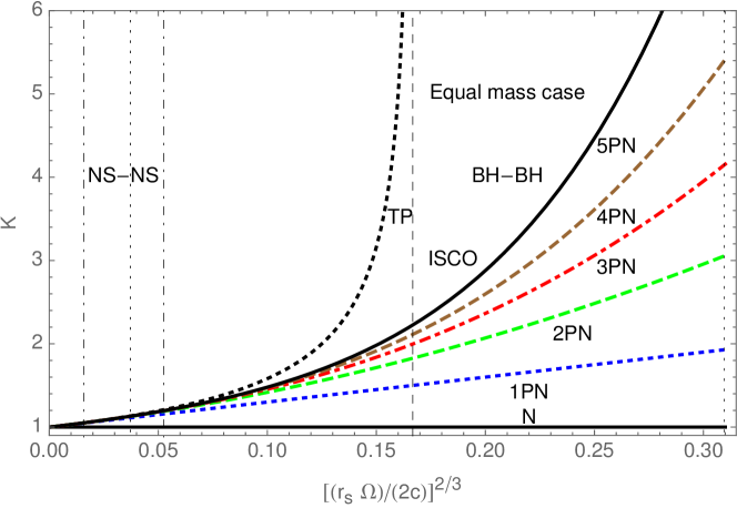
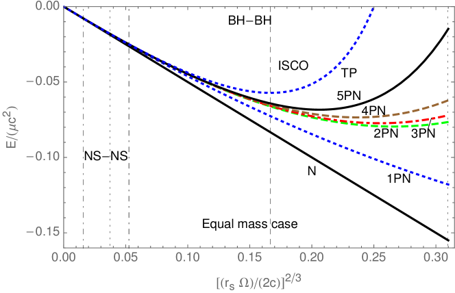
We illustrate the different post–Newtonian contributions to the binding energy, $E^{\rm circ}(x)$, and the periastron advance, $K^{\rm circ}(x)$ for circular orbits, setting $m_{1}=m_{2},\leavevmode\nobreak\ \leavevmode\nobreak\ (\nu=1/4)$, with $x=(G_{N}M\Omega/c^{3})^{2/3}$, $\Omega=\Omega_{\phi}$ the angular frequency, and $r_{s}$ the Schwarzschild radius. The relation between $j$ and $x$ to 5PN is given by

$$j = \frac{1}{\sqrt{x}}\Biggl{\{}1+\frac{1}{6}\eta^{2}x(9+\nu)+\frac{1}{24}\eta^{4}x^{2}\big{(}81-57\nu+\nu^{2}\big{)}+\eta^{6}x^{3}\Bigg{[}\frac{135}{16}+\frac{1}{144}\big{(}-6889+246\pi^{2}\big{)}\nu$$ (83)

$$+\frac{31\nu^{2}}{24}+\frac{7\nu^{3}}{1296}\Biggr{]}+\eta^{8}x^{4}\Biggl{[}\frac{2835}{128}+\nu\Biggl{(}\frac{98869}{5760}-\frac{128\gamma_{E}}{3}-\frac{6455\pi^{2}}{1536}-\frac{256\ln(2)}{3}-\frac{64\ln(x)}{3}\Biggr{)}$$

$$+\frac{5\big{(}71207-2706\pi^{2}\big{)}}{3456}\nu^{2}-\frac{215\nu^{3}}{1728}-\frac{55\nu^{4}}{31104}\Biggr{]}+\eta^{10}x^{5}\Biggl{[}\frac{15309}{256}+\Biggl{(}\frac{59112343}{44800}+\frac{19952\gamma_{E}}{105}$$

$$-\frac{126779\pi^{2}}{768}+\frac{47344\ln(2)}{105}-\frac{486\ln(3)}{7}+\frac{9976\ln(x)}{105}\Biggr{)}\nu+\Biggl{(}{\frac{99980267}{50400}}+\frac{2624\gamma_{E}}{15}$$

$$-\frac{289595\pi^{2}}{1536}+\frac{6976\ln(2)}{105}+\frac{1944\ln(3)}{7}+\frac{1312\ln(x)}{15}\Biggr{)}\nu^{2}+\frac{1}{256}\nu^{3}\big{(}-25189+902\pi^{2}\big{)}$$

$$-\frac{55\nu^{4}}{768}-\frac{\nu^{5}}{768}\Biggr{]}\Biggr{\}}+O(\eta^{12}).$$

We also add the the test–particle lines (TP), which are given by [80]

$$\frac{E^{\rm circ}_{\rm TP}}{\mu c^{2}} = \frac{1-2x\eta^{2}}{\sqrt{1-3x\eta^{2}}}-1$$ (84)

and

$$K_{\rm TP}^{\rm circ} = \frac{1}{\sqrt{1-6\eta^{2}x}}$$ (85)

with

$$j_{\rm TP}=\frac{1}{\sqrt{x(1-3\eta^{2}x)}}.$$ (86)

The different post–Newtonian corrections are all positive correcting lower order results. Even at 5PN the convergence is not yet perfect both for the binding energy and periastron advance, considering the range $x\in[0,0.30]$, which is calling for effective resummations of these contributions. We also mention that the post–Minkowskian corrections to $O(G_{N}^{4})$ given in [68] recently represent the bound state dynamics to the 3rd post–Newtonian order. Starting with 4PN there are deviations both in the potential and tail terms, because of the yet missing higher powers in $1/r$ and also the fact that these corrections are derived for scattering kinematics, still to be kinematically continued to the elliptic orbit kinematics. On the other hand, our formalism allowed to predict the post–Newtonian expansion terms of the results of [68] up to 6PN, cf. [20, 77]

Finally, we present the PN–expansion of the local scattering angle, cf. (48–50).

$$\chi_{1}^{\rm h,loc} = \frac{w_{1}}{2p_{\infty}}=\frac{1}{p_{\infty}}+2\eta^{2}p_{\infty},$$ (87)

$$\chi_{2}^{\rm h,loc} = \pi\frac{w_{2}}{4}=\pi\Biggl{[}\frac{3\eta^{2}}{2}+\frac{3}{8}\eta^{4}(5-2\nu)p_{\infty}^{2}+\frac{3}{16}\eta^{6}\nu(-4+3\nu)p_{\infty}^{4}+\eta^{8}\Biggl{(}\frac{9\nu}{64}+\frac{27\nu^{2}}{64}-\frac{15\nu^{3}}{32}\Biggr{)}p_{\infty}^{6}$$ (88)

$$+\eta^{10}\Biggl{(}-\frac{15\nu}{256}-\frac{45\nu^{2}}{256}-\frac{15\nu^{3}}{64}+\frac{105\nu^{4}}{256}\Biggr{)}p_{\infty}^{8}\Biggr{]},$$

$$\chi_{3}^{\rm h,loc} = -\frac{w_{1}^{3}}{24p_{\infty}^{3}}+\frac{w_{1}w_{2}}{2p_{\infty}}+w_{3}p_{\infty},$$ (89)

$$\chi_{4}^{\rm h,loc} = \pi\left(\frac{3w_{2}^{2}}{16}+\frac{3w_{1}w_{3}}{8}+\frac{3w_{4}}{8}p_{\infty}^{2}\right),$$ (90)

$$\chi_{5}^{\rm h,loc} = \frac{w_{1}^{5}}{160p_{\infty}^{5}}-\frac{w_{1}^{3}w_{2}}{12p_{\infty}^{3}}+\frac{w_{1}^{2}w_{3}+w_{1}w_{2}^{2}}{2p_{\infty}}+\left(2w_{2}w_{3}+2w_{1}w_{4}\right)p_{\infty}+\frac{4w_{5}}{3}p_{\infty}^{3}$$ (91)

$$= \frac{1}{5p_{\infty}^{5}}-\frac{2\eta^{2}}{p_{\infty}^{3}}+\frac{8\eta^{4}(4-\nu)}{p_{\infty}}+\eta^{6}p_{\infty}\left(320-\left(\frac{1168}{3}-\frac{41\pi^{2}}{8}\right)\nu+24\nu^{2}\right)$$

$$+\eta^{8}p_{\infty}^{3}\left(640-\frac{3632944-76035\pi^{2}}{2160}\nu+\frac{1}{72}\big{(}58736-861\pi^{2}\big{)}\nu^{2}-40\nu^{3}\right)$$

$$+\eta^{10}p_{\infty}^{5}\Biggl{(}\frac{1792}{5}-\frac{93470656-3886715\pi^{2}}{33600}\nu+\left({\frac{64770686}{14175}}-\frac{107249}{480}\right)\nu^{2}$$

$$-\frac{1}{72}\big{(}88864-1353\pi^{2}\big{)}\nu^{3}+56\nu^{4}\Biggr{)},$$

$$\chi_{6}^{\rm h,loc} = \pi\Biggl{[}\frac{5w_{2}^{3}}{32}+\frac{15w_{1}w_{2}w_{3}}{16}+\frac{15w_{1}^{2}w^{4}}{32}+\left(\frac{15w_{3}^{2}}{32}+\frac{15w_{2}w_{4}}{16}+\frac{15w_{1}w_{5}}{16}\right)p_{\infty}^{2}+\frac{15w_{6}}{32}p_{\infty}^{4}\Biggr{]}$$ (92)

$$= \pi\Biggl{[}\eta^{6}\left(\frac{1155}{8}-\left(\frac{625}{4}-\frac{615\pi^{2}}{256}\right)\nu+\frac{105}{16}\nu^{2}\right)+\eta^{8}p_{\infty}^{2}\Biggl{(}\frac{45045}{64}-\frac{37556864-771585\pi^{2}}{24576}\nu$$

$$+\frac{5}{64}\big{(}7013-123\pi^{2}\big{)}\nu^{2}-\frac{525}{32}\nu^{3}\Biggr{)}+\eta^{10}p_{\infty}^{4}\Biggl{(}\frac{135135}{128}-\frac{8099529344-243724425\pi^{2}}{1720320}\nu$$

$$+\left({\frac{288262859}{40320}-\frac{13335615}{32768}\pi^{2}}\right)\nu^{2}-\frac{25\big{(}87872-1599\pi^{2}\big{)}}{2048}\nu^{3}+\frac{3675}{128}\nu^{4}\Biggr{)}\Biggr{]}.$$

The parameters $w_{i}$ the expansions need to be expanded up to $O(p_{\infty}^{8})$ in accordance with 5PN accuracy,

$$w_{i} = \sum_{k=0}^{4}v_{i,k}(\nu)p_{\infty}^{2k}$$ (93)

and can be obtained recursively from (87–92). For $\chi_{3,4}^{\rm h,loc}$ the explicit expressions are given in (LABEL:eq:chi31, 72). Leaving the 5PN EOB parameters open, one obtains

$$\chi_{2}^{{\rm h,loc},p_{\infty}^{8}} = -\pi\eta^{10}p_{\infty}^{8}\frac{35}{512}q_{82}$$ (94)

$$\chi_{3}^{{\rm h,loc},p_{\infty}^{7}} = \eta^{10}p_{\infty}^{7}\left(\frac{18\nu}{5}+\frac{54\nu^{2}}{5}-12\nu^{3}-\frac{1}{7}q_{63}-q_{82}\right)$$ (95)

$$\chi_{4}^{{\rm h,loc},p_{\infty}^{6}} = \pi\eta^{10}p_{\infty}^{6}\left(-\frac{1971}{64}\nu+\frac{5601}{64}\nu^{2}-\frac{975}{32}\nu^{3}-\frac{3}{64}q_{44}-\frac{15}{64}q_{63}-\frac{105}{128}q_{82}\right)$$ (96)

$$\chi_{5}^{{\rm h,loc},p_{\infty}^{5}} = \eta^{10}p_{\infty}^{5}\left(\frac{1792}{5}-\frac{415658\nu}{225}+\frac{32492\nu^{2}}{15}-\frac{1896\nu^{3}}{5}-\frac{1}{120}\nu(-4085+1722\nu)\pi^{2}\right.$$ (97)

$$\left.-\frac{4}{15}\bar{d}_{5}-\frac{4}{5}q_{44}-2q_{63}-\frac{14}{3}q_{82}\right)$$

$$\chi_{6}^{{\rm h,loc},p_{\infty}^{4}} = \eta^{10}p_{\infty}^{4}\pi\left[\frac{135135}{128}+\left(-\frac{180377}{48}+\frac{1283765\pi^{2}}{16384}\right)\nu+\left(\frac{190655}{64}-\frac{36285\pi^{2}}{1024}\right)\nu^{2}\right.$$ (98)

$$\left.-\frac{9945}{32}\nu^{3}-\frac{15}{32}a_{6}-\frac{15}{32}\bar{d}_{5}-\frac{45}{64}q_{44}-\frac{75}{64}q_{63}-\frac{525}{256}q_{82}\right].$$

The other parts are determined by the 4PN contributions.

If we consider the phenomenological addition, Eq. (77), the following changes are implied. Let $X$ be one of the following observables and the change $\delta X$ defined by

$$\delta X=X(H)-X(H+\delta H_{\text{{rad}}}).$$ (99)

Then one obtains

$$\delta K(\hat{E},j)^{\rm 5PN}_{\rm loc,h}\leavevmode\nobreak\ = \leavevmode\nobreak\ a\eta^{10}\nu^{2}\left[\frac{63}{16j^{10}}+\frac{105\hat{E}}{8j^{8}}+\frac{45\hat{E}^{2}}{4j^{6}}+\frac{3\hat{E}^{3}}{2j^{4}}\right],$$ (100)

$$\delta E^{\rm circ}(j)\leavevmode\nobreak\ = \leavevmode\nobreak\ 0,$$ (101)

$$\delta K^{\rm circ}(j)\leavevmode\nobreak\ = \leavevmode\nobreak\ 0,$$ (102)

$$\delta j(x)\leavevmode\nobreak\ = \leavevmode\nobreak\ 0,$$ (103)

$$\delta\chi_{4}^{\rm h,loc}\leavevmode\nobreak\ = \leavevmode\nobreak\ a\pi\eta^{10}\nu^{2}\frac{3}{32}p_{\infty}^{6},\leavevmode\nobreak\ \leavevmode\nobreak\ \text{\rm etc.},$$ (104)

which, again, is a consequence of the transformation of $q_{44}$ only. The expressions for $\chi_{k}^{\rm h},\leavevmode\nobreak\ k=1,2,3$ remain the same. Yet no consistent solution demanding the constraint (75) and referring to the Hamiltonian in the multipole–picture for the far-zone terms is obtained.

5 Conclusions

We have calculated the 5PN Hamiltonian in the harmonic gauge using an EFT method both for the potential and the far-zone terms. For the memory term we obtain a different result comparing to [30] and find one more contributing diagram. From the local contributions to periastron advance $K^{\rm loc,h}(\hat{E},j)$ it has been possible to derive the five 5PN EOB parameters $q_{82},q_{63},q_{44},\bar{d}_{5}$ and $a_{6}$. The rational contributions of $O(\nu^{2})$ to $q_{44},\bar{d}_{5}$ and $a_{6}$ do also depend on the non–singular multipole moments $L_{k}\varepsilon_{ijk}Q_{il}Q_{jl}$ and $Q_{ij}Q_{jk}Q_{ki}$, which enter as $D=4$ dependent quantities and are of $O(\nu^{2})$. We are not aware of other far-zone contributions in the EFT approach.

Our results on the observables $K^{\rm loc,h}(\hat{E},j)$, the total circular peristron advance $K^{\rm tot}(j)$, the circular binding energy $E^{\rm circ}$ and the contributions to the scattering angle $\chi_{k},\leavevmode\nobreak\ \leavevmode\nobreak\ k\in[1,6]$, do agree with the results of Ref. [15], in the case of the parameters given there, except of the rational $O(\nu^{2})$ term of $q_{44}$. Furthermore, we have also newly obtained the rational contributions of $O(\nu^{2})$ to $\bar{d}_{5}$ and $a_{6}$ for the first time. The $O(\nu^{2}\pi^{2})$ contributions to $q_{44}$ were obtained in [14] and those to $\bar{d}_{5}$ and $a_{6}$ in [16] before. These terms stem from the potential contributions. For them the relation (75) holds. Our calculation of the 5PN Hamiltonian ab initio leads to a violation of relation (75) for the $O(\nu^{2})$ rational term in $q_{44}$. As has been outlined in Section 4, the results of [14] could be obtained by invoking the additional term (77, 79) changing only $q_{44}$, but leaving $\bar{d}_{5}$ and $a_{6}$ invariant. We presented numerical results to 5PN for $E^{\rm circ}$ and $K^{\rm circ}$.

We are aware of the fact that one may perform resummations of the exact results obtained for the Hamiltonian dynamics to a certain post–Newtonian order, see e.g. [81, 75], even with a matching to results from numerical gravity, to be performed in a gauge invariant way. However, it is well–known that resummations of this kind, also applied in phenomenological implementations of exact quantum field theoretic calculations sometimes, cannot accommodate for exact results, since some of the higher order corrections are necessarily not included. The latter ones may be of the same order or even larger than the resummed terms. One example can be found in Ref. [82].

The level of the 5PN corrections to Hamiltonian dynamics exhibits a complexity which currently could only be solved using the effective field theory approach. The latter has been originally developed for renormalizable quantum field theories. There refined algorithms for the automated computer algebraic derivation of all dynamical contributions and very efficient algorithms for term reduction exist [34, 33]. Likewise, many methods to compute the contributing integrals analytically have been developed [73]. By these methods the problem at hand could be solved. Any theory having a path integral representation, including classical mechanics, can be formulated in this way. Here the path integral [63] is a consequence of the variational principles of mechanics [83], the basis of any dynamical physical law. Symbioses of different fields in science lead to progress in the present case. Future calculations will use similar technologies at higher post-Newtonian orders. Given the fast growth of complexity, however, even more refined technologies have to be developed to solve these problems.

Appendix A The Feynman rules and integrals

In the following we list the Feynman rules, which are necessary to calculate the convergent far-zone contributions. We first present the Feynman rules in the standard case [4] and turn then to those in the in–in formalism.

$$\phi:\raisebox{-14.51091pt}{\includegraphics{phiprop}}={} -\frac{i}{2c_{d}}D(p)\,,$$ (105)

$$A:\raisebox{-14.51091pt}{\includegraphics{Aprop}}={} \frac{i\delta_{ij}}{2}D(p)\,,$$ (106)

$$\sigma:\raisebox{-14.51091pt}{\includegraphics{sigmaprop}}={} -\frac{i}{2}D(p)[\delta_{i_{1}j_{1}}\delta_{i_{2}j_{2}}+\delta_{i_{1}j_{2}}\delta_{i_{2}j_{1}}+(2-c_{d})\delta_{i_{1}i_{2}}\delta_{j_{1}j_{2}}]\,,$$ (107)

$$\vbox{\hbox{\includegraphics{vphibinary}}}={} -\frac{i}{\Lambda}\biggl{(}E{-}\frac{1}{2}Q_{ij}p_{i}p_{j}{-}\frac{i}{6}O_{ijk}p_{i}p_{j}p_{k}\biggr{)}\,,$$ (108)

$$\vbox{\hbox{\includegraphics{vAbinary}}}={} \frac{i}{\Lambda}\biggl{(}-\frac{i}{2}L_{j}\varepsilon_{ijk}p_{k}{-}\frac{1}{2}Q_{ij}p_{0}p_{j}+\frac{1}{3}J_{jk}\varepsilon_{ijl}p_{k}p_{l}{-}\frac{i}{6}O_{ijk}p_{j}p_{k}p_{0}\biggr{)}\,,$$ (109)

$$\vbox{\hbox{\includegraphics{vsigmabinary}}}={} \frac{i}{\Lambda}\biggl{(}-\frac{1}{4}Q_{ij}p_{0}^{2}+\frac{1}{6}(J_{ik}\varepsilon_{jkl}+J_{jk}\varepsilon_{ikl})p_{l}p_{0}{-}\frac{i}{12}O_{ijk}p_{k}p_{0}^{2}\biggr{)}\,,$$ (110)

$$\vbox{\hbox{\includegraphics{vsigmasigmabinary}}}={} \begin{aligned} \tfrac{i}{16\Lambda^{2}}p_{10}p_{20}(&\delta_{i_{1}i_{2}}Q_{j_{1}j_{2}}+\delta_{i_{1}j_{2}}Q_{i_{2}j_{1}}\\ &+\delta_{i_{2}j_{1}}Q_{i_{1}j_{2}}+\delta_{j_{1}j_{2}}Q_{i_{1}i_{2}}+\dots)\,,\end{aligned}$$ (111)

$$\vbox{\hbox{\includegraphics{vphiphiphi}}}={} \frac{2ic_{d}^{2}}{\Lambda}(p_{10}p_{20}+p_{10}p_{30}+p_{20}p_{30})\,,$$ (112)

$$\vbox{\hbox{\includegraphics{vphiphiA}}}={} -\frac{2ic_{d}}{\Lambda}(p_{10}p_{2i_{3}}+p_{1i_{3}}p_{20})\,,$$ (113)

$$\vbox{\hbox{\includegraphics{vphiphisigma}}}={} \frac{ic_{d}}{\Lambda}(-p_{1_{3}i}p_{2j_{3}}-p_{1j_{3}}p_{2i_{3}}+\delta_{i_{3}j_{3}}p_{1}\cdot p_{2})\,,$$ (114)

$$\vbox{\hbox{\includegraphics{vphiAA}}}={} \frac{2ic_{d}}{\Lambda}(-p_{2i_{2}}p_{3i_{3}}+p_{2i_{3}}p_{3i_{2}}-2\delta_{i_{2}i_{3}}p_{2i}p_{3i})\,,$$ (115)

$$\vbox{\hbox{\includegraphics{vphiAsigma}}}={} \begin{aligned} \tfrac{ic_{d}}{\Lambda}(&-\delta_{i_{3}i_{2}}p_{10}p_{2i_{3}}+\delta_{i_{3}i_{2}}p_{1j_{3}}p_{20}+\delta_{i_{3}j_{3}}p_{10}p_{2i_{2}}\\ &-\delta_{i_{3}j_{3}}p_{1i_{2}}p_{20}-\delta_{i_{2}j_{3}}p_{10}p_{2i_{3}}+\delta_{i_{2}j_{3}}p_{1i_{3}}p_{20})\,,\end{aligned}$$ (116)

$$\vbox{\hbox{\includegraphics{vphisigmasigma}}}={} \frac{ic_{d}}{2\Lambda}p_{20}p_{30}(\delta_{i_{2}i_{3}}\delta_{j_{2}j_{3}}-\delta_{i_{2}j_{2}}\delta_{i_{3}j_{3}}+\delta_{i_{2}j_{3}}\delta_{i_{3}j_{2}})\,,$$ (117)

$$\vbox{\hbox{\includegraphics{vAAA}}}={} \begin{aligned} \tfrac{2i}{\Lambda}(&-\delta_{i_{1}i_{2}}p_{10}p_{2i_{3}}-\delta_{i_{1}i_{2}}p_{10}p_{3i_{3}}+\delta_{i_{1}i_{2}}p_{1i_{3}}p_{20}+\delta_{i_{1}i_{2}}p_{1i_{3}}p_{30}\\ &+\delta_{i_{1}i_{2}}p_{20}p_{3i_{3}}+\delta_{i_{1}i_{2}}p_{2i_{3}}p_{30}+\delta_{i_{1}i_{3}}p_{10}p_{2i_{2}}+\delta_{i_{1}i_{3}}p_{10}p_{3i_{2}}\\ &-\delta_{i_{1}i_{3}}p_{1i_{2}}p_{20}+\delta_{i_{1}i_{3}}p_{1i_{2}}p_{30}-\delta_{i_{1}i_{3}}p_{20}p_{3i_{2}}+\delta_{i_{1}i_{3}}p_{2i_{2}}p_{30}\\ &+\delta_{i_{2}i_{3}}p_{10}p_{2i_{1}}+\delta_{i_{2}i_{3}}p_{10}p_{3i_{1}}+\delta_{i_{2}i_{3}}p_{1i_{1}}p_{20}-\delta_{i_{2}i_{3}}p_{1i_{1}}p_{30}\\ &+\delta_{i_{2}i_{3}}p_{20}p_{3i_{1}}-\delta_{i_{2}i_{3}}p_{2i_{1}}p_{30})\,,\end{aligned}$$ (118)

$$\vbox{\hbox{\includegraphics{vAAsigma}}}={} \begin{aligned} \tfrac{i}{\Lambda}(&p_{1}\cdot p_{2}(-\delta_{i_{1}i_{2}}\delta_{i_{3}j_{3}}+\delta_{i_{1}i_{3}}\delta_{i_{2}j_{3}}+\delta_{i_{2}i_{3}}\delta_{i_{1}j_{3}})\\ &+\delta_{i_{1}i_{2}}(p_{1i_{3}}p_{2j_{3}}+p_{1j_{3}}p_{2i_{3}})+\delta_{i_{1}i_{3}}(p_{1i_{2}}p_{2j_{3}}-p_{1j_{3}}p_{2i_{2}})\\ &-\delta_{i_{2}i_{3}}(p_{1i_{1}}p_{2j_{3}}-p_{1j_{3}}p_{2i_{1}})+\delta_{i_{1}j_{3}}(p_{1i_{2}}p_{2i_{3}}-p_{1i_{3}}p_{2i_{2}})\\ &-\delta_{i_{2}j_{3}}(p_{1i_{1}}p_{2i_{3}}-p_{1i_{3}}p_{2i_{1}})+\delta_{i_{3}j_{3}}(p_{1i_{1}}p_{2i_{2}}-p_{1i_{2}}p_{2i_{1}}))\,,\end{aligned}$$ (119)

$$\vbox{\hbox{\includegraphics{vAsigmasigma}}}={} \frac{i}{8\Lambda}(V^{A\sigma\sigma}_{i_{1},i_{2}j_{2},i_{3}j_{3}}+V^{A\sigma\sigma}_{i_{1},i_{2}j_{2},j_{3}i_{3}}+V^{A\sigma\sigma}_{i_{1},j_{2}i_{2},i_{3}j_{3}}+V^{A\sigma\sigma}_{i_{1},j_{2}i_{2},j_{3}i_{3}})$$ (120)

$$V^{A\sigma\sigma}_{i_{1},i_{2}j_{2},i_{3}j_{3}}={} \delta_{i_{2}i_{3}}\delta_{j_{2}j_{3}}[4p_{20}p_{2i_{1}}+2(p_{1i_{1}}p_{20}+p_{10}p_{2i_{1}})]+\delta_{i_{3}j_{3}}[-2p_{20}(\delta_{i_{1}i_{2}}p_{1j_{2}}$$

$$+\delta_{i_{2}j_{2}}p_{2i_{1}})-\delta_{i_{2}j_{2}}(p_{1i_{1}}p_{20}+p_{10}p_{2i_{1}})]+\delta_{i_{1}i_{2}}[2\delta_{i_{3}j_{3}}p_{10}p_{2j_{2}}$$

$$+\delta_{i_{3}j_{2}}(4p_{1j_{3}}p_{20}-4p_{10}p_{2j_{3}})]+\delta_{i_{1}i_{3}}[\delta_{i_{2}j_{3}}(-4p_{1j_{2}}p_{20}$$

$$+4p_{10}p_{2j_{2}})+\delta_{i_{2}j_{2}}(2p_{1j_{3}}p_{20}-2p_{10}p_{2j_{3}})]$$ (121)

$$\vbox{\hbox{\includegraphics{vsigmasigmasigma}}}={} \frac{i}{32\Lambda}(\tilde{V}^{\sigma\sigma\sigma}_{i_{1}j_{1},i_{2}j_{2},i_{3}j_{3}}+\tilde{V}^{\sigma\sigma\sigma}_{j_{1}i_{1},i_{2}j_{2},i_{3}j_{3}})$$ (122)

$$\tilde{V}^{\sigma\sigma\sigma}_{i_{1}j_{1},i_{2}j_{2},i_{3}j_{3}}={} V^{\sigma\sigma\sigma}_{i_{1}j_{1},i_{2}j_{2},i_{3}j_{3}}+V^{\sigma\sigma\sigma}_{i_{1}j_{1},j_{2}i_{2},i_{3}j_{3}}+V^{\sigma\sigma\sigma}_{i_{1}j_{1},i_{2}j_{2},j_{3}i_{3}}+V^{\sigma\sigma\sigma}_{i_{1}j_{1},j_{2}i_{2},j_{3}i_{3}}$$ (123)

$$V^{\sigma\sigma\sigma}_{i_{1}j_{1},i_{2}j_{2},i_{3}j_{3}}={} ({p}_{1}^{2}+{p}_{1}\cdot{p}_{2}+{p}_{2}^{2})\*\Bigl{(}-\delta_{i_{2}j_{2}}\*\bigl{(}2\*\delta_{i_{1}i_{3}}\*\delta_{j_{1}j_{3}}-\delta_{i_{1}j_{1}}\*\delta_{i_{3}j_{3}}\bigr{)}$$

$$\quad+2\*\bigl{[}\delta_{i_{1}i_{2}}\*\bigl{(}4\*\delta_{j_{1}i_{3}}\*\delta_{j_{2}j_{3}}-\delta_{j_{1}j_{2}}\*\delta_{i_{3}j_{3}}\bigr{)}-\delta_{i_{1}j_{1}}\*\delta_{i_{2}i_{3}}\*\delta_{j_{2}j_{3}}\bigr{]}\Bigr{)}$$

$$+2\*\Bigl{\{}4\*\bigl{(}p_{1j_{3}}\*p_{2j_{1}}-p_{1j_{1}}\*p_{2j_{3}}\bigr{)}\*\delta_{i_{1}i_{2}}\*\delta_{j_{2}i_{3}}$$

$$\quad+2\*\bigl{[}\bigl{(}p_{1i_{1}}+p_{2i_{1}}\bigr{)}\*p_{2j_{1}}\*\delta_{i_{2}i_{3}}\*\delta_{j_{2}j_{3}}-p_{1i_{3}}\*p_{2j_{3}}\*\delta_{i_{1}i_{2}}\*\delta_{j_{1}j_{2}}\bigr{]}$$

$$\quad+\delta_{i_{2}j_{2}}\*\bigl{[}p_{1i_{3}}\*p_{2j_{3}}\*\delta_{i_{1}j_{1}}+2\*\bigl{(}p_{1j_{3}}\*p_{2j_{1}}-p_{1j_{1}}\*p_{2j_{3}}\bigr{)}\*\delta_{i_{1}i_{3}}$$

$$\quad-\bigl{(}p_{1i_{1}}+p_{2i_{1}}\bigr{)}\*p_{2j_{1}}\*\delta_{i_{3}j_{3}}\bigr{]}$$

$$\quad+p_{2j_{2}}\*\Bigl{(}4\*p_{1j_{1}}\*\delta_{i_{1}i_{3}}\*\delta_{i_{2}j_{3}}+p_{1i_{2}}\*\bigl{(}2\*\delta_{i_{1}i_{3}}\*\delta_{j_{1}j_{3}}-\delta_{i_{1}j_{1}}\*\delta_{i_{3}j_{3}}\bigr{)}$$

$$\qquad+2\*\bigl{[}\delta_{i_{1}i_{2}}\*\bigl{(}p_{1j_{1}}\*\delta_{i_{3}j_{3}}-2\*p_{1j_{3}}\*\delta_{j_{1}i_{3}}\bigr{)}-p_{1j_{3}}\*\delta_{i_{1}j_{1}}\*\delta_{i_{2}i_{3}}\bigr{]}\Bigr{)}$$

$$\quad+p_{1j_{2}}\*\Bigl{(}p_{1i_{2}}\*\bigl{(}2\*\delta_{i_{1}i_{3}}\*\delta_{j_{1}j_{3}}-\delta_{i_{1}j_{1}}\*\delta_{i_{3}j_{3}}\bigr{)}-4\*p_{2j_{1}}\*\delta_{i_{1}i_{3}}\*\delta_{i_{2}j_{3}}$$

$$\qquad+2\*\bigl{[}p_{2j_{3}}\*\delta_{i_{1}j_{1}}\*\delta_{i_{2}i_{3}}+\delta_{i_{1}i_{2}}\*\bigl{(}2\*p_{2j_{3}}\*\delta_{j_{1}i_{3}}-p_{2j_{1}}\*\delta_{i_{3}j_{3}}\bigr{)}\bigr{]}\Bigr{)}\Bigr{\}},$$ (124)

with

$$c_{d}=\frac{2(d-1)}{d-2},$$ (125)

$\Lambda^{-1}=\sqrt{32\pi G_{N}}$ and $d=3-2\varepsilon$. The scalar propagators $D(p)$ are left generic and will be specified either as causal, retarded, or advanced propagators, cf. Section B. Furthermore, in the specific in–in calculations below one has to replace in (110, 111) for the electric quadrupole moment the vertices as given in (159–161). Furthermore, we list the contributing field combinations in Table 1.

Eq.	contributions
(112), (118), (122)	$++-,---$
(113), (114), (119)	$++-,+-+,---$
(115), (117), (120)	$++-,-++,---$
(116)	$++-,+-+,-++,---$

Table 1: The contributing field combinations in the in–in formalism.

Here the bulk vertices have to be rescaled by $1/\sqrt{2}$. The free–field combinations are defined in Eq. (155).

The $D$–dimensional integral over an Euclidean momentum $k_{E}$ is given by, cf. e.g. [84],

$$\int\frac{d^{D}\vec{k}_{E}}{(2\pi)^{D}}\frac{(\vec{k}^{2}_{E})^{r}}{(\vec{k}^{2}_{E}+R^{2})^{m}}=\frac{(-1)^{r-m}}{(4\pi)^{D/2}}\frac{\Gamma(r+D/2)}{\Gamma(D/2)}\Gamma(m-r-D/2)(R^{2})^{D/2+r-m}.$$ (126)

Appendix B Invariant functions

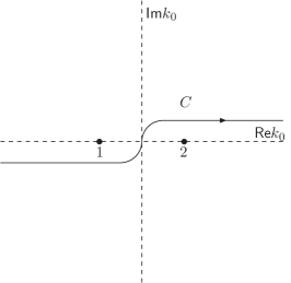
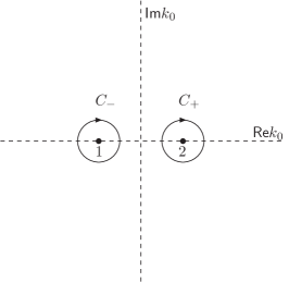
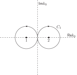
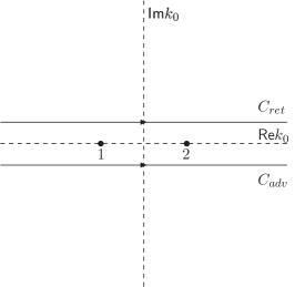
In the following we summarize different functions, related to the scalar field operators $\Phi(x_{1})$ and $\Phi(x_{2})$, and $x=x_{1}-x_{2}$, leading to the different kind of propagators, [85], which are distribution–valued in part [86, 87]. The corresponding contours for the defining integrals are shown in Figure 4.

We start with the commutator

$$i\Delta(x)=[\Phi(x_{1}),\Phi(x_{2})]_{-}=-i\int\frac{d^{D-1}k}{(2\pi)^{D-1}}\frac{1}{\omega_{k}}\frac{e^{-ikx}}{k^{2}-m^{2}},$$ (127)

with $\omega_{k}=\sqrt{\vec{k}^{2}+m^{2}}$, denoting the Jordan–Pauli function [88]. It has the contour integral representation

$$\Delta(x) = \int_{C_{0}}\frac{d^{D}k}{(2\pi)^{D}}\frac{e^{ik.x}}{k^{2}-m^{2}}=\Delta_{+}(x)+\Delta_{-}(x)=\Delta_{\rm ret}(x)-\Delta_{\rm adv}(x),$$ (128)

showing also the relation to other quantities

$$\Delta_{1}(x) = \int_{C_{1}}\frac{d^{D}k}{(2\pi)^{D}}\frac{e^{ik.x}}{k^{2}-m^{2}}=\Delta_{+}(x)-\Delta_{-}(x)$$ (130)

$$\Delta_{\pm}(x) = \int_{C_{\pm}}\frac{d^{D}k}{(2\pi)^{D}}\frac{e^{ik.x}}{k^{2}-m^{2}}=\frac{1}{2}\left[\Delta(x)\pm\Delta_{1}(x)\right],$$ (131)

$$\Delta_{c}(x) = -i\int_{C}\frac{d^{D}k}{(2\pi)^{D}}\frac{e^{ik.x}}{k^{2}-m^{2}}=-i\left[\Theta(t)\Delta_{+}(x)+\Theta(-t)\Delta_{-}(x)\right],$$

$$\Delta_{D}(x) = -i\left[\Theta(t)\Delta_{-}(x)+\Theta(-t)\Delta_{+}(x)\right],$$

$$\Delta_{\rm ret}(x) = \int_{C_{\rm ret}}\frac{d^{D}k}{(2\pi)^{D}}\frac{e^{ik.x}}{k^{2}-m^{2}}=\Theta(t)\Delta(x),$$ (134)

$$\Delta_{\rm adv}(x) = \int_{C_{\rm adv}}\frac{d^{D}k}{(2\pi)^{D}}\frac{e^{ik.x}}{k^{2}-m^{2}}=-\Theta(-t)\Delta(x),$$ (135)

with $\Theta(t)$ the Heaviside function.

The causal Green’s function $\Delta_{c}(x)$ [89] is also called Feynman function $\Delta_{F}(x)$ and the Dyson function $\Delta_{D}(x)$ is also called anti–causal Green’s function.

In momentum space the causal, retarded and advanced propagators read

$$\Delta_{c}(k)\leavevmode\nobreak\ = \leavevmode\nobreak\ \frac{1}{k^{2}-m^{2}+i0},$$ (136)

$$\Delta_{\rm ret}(k)\leavevmode\nobreak\ = \leavevmode\nobreak\ \frac{1}{k^{2}-m^{2}+(2k_{0})i0},$$ (137)

$$\Delta_{\rm adv}(k)\leavevmode\nobreak\ = \leavevmode\nobreak\ \frac{1}{k^{2}-m^{2}-(2k_{0})i0},$$ (138)

where the distribution relations [90, 86, 87]

$$\frac{1}{x\pm i0}={\cal P}\frac{1}{x}\mp i\pi\delta(x)$$ (139)

hold, with ${\cal P}$ Cauchy’s principal value.

Figure 4: The integration paths in the complex $k_{0}$ plane for the different types of propagator functions. The paths correspond to the integrals given in the text and correspond to the causal Green’s function $(C)$, the Jordan–Pauli function $(C_{0})$, the two Wightman functions $(C_{\pm})$, the anticommutator $(C_{1})$, and the retarded and advanced Green’s functions $(C_{\rm ret(adv)})$, where $C_{1}$ denotes a single path.

Appendix C The in-in formalism

The in–in formalism for binary systems in classical gravity refers to a well–defined initial state at $t=-\infty$, which is also defined to be the final state, and one integrates over the time paths $t_{F}$ and $t_{B}$

$$t_{F}\leavevmode\nobreak\ =\leavevmode\nobreak\ (-\infty,+\infty),\leavevmode\nobreak\ \leavevmode\nobreak\ \leavevmode\nobreak\ \leavevmode\nobreak\ \leavevmode\nobreak\ \leavevmode\nobreak\ \leavevmode\nobreak\ t_{B}\leavevmode\nobreak\ =\leavevmode\nobreak\ (+\infty,-\infty),$$ (140)

which are linked together, with $t_{F}=t_{1}$ and $t_{B}=t_{2}$ labeling the time path. One should note that different authors use a quite different notation. For definiteness we refer to the one by Keldysh [52] also given in [55]. In the following 2–dimensional representations the Pauli matrices

$$\sigma_{1}\leavevmode\nobreak\ =\leavevmode\nobreak\ \left(\begin{array}[]{rr}0\nobreak\leavevmode\nobreak\leavevmode&\leavevmode\nobreak\ \leavevmode\nobreak\ 1\\ 1\nobreak\leavevmode\nobreak\leavevmode&\leavevmode\nobreak\ \leavevmode\nobreak\ 0\end{array}\right),\leavevmode\nobreak\ \leavevmode\nobreak\ \leavevmode\nobreak\ \leavevmode\nobreak\ \leavevmode\nobreak\ \sigma_{2}\leavevmode\nobreak\ =\leavevmode\nobreak\ \left(\begin{array}[]{rr}0\nobreak\leavevmode&\leavevmode\nobreak\ -i\\ i\nobreak\leavevmode&\leavevmode\nobreak\ 0\end{array}\right),\leavevmode\nobreak\ \leavevmode\nobreak\ \leavevmode\nobreak\ \leavevmode\nobreak\ \leavevmode\nobreak\ \sigma_{3}\leavevmode\nobreak\ =\leavevmode\nobreak\ \left(\begin{array}[]{rr}1\nobreak\leavevmode&\leavevmode\nobreak\ 0\\ 0\nobreak\leavevmode&\leavevmode\nobreak\ -1\end{array}\right)$$ (147)

are of use. One has

$$\left(\begin{array}[]{c}\Psi_{1}\\ \Psi_{2}\end{array}\right)=\frac{1}{\sqrt{2}}(1+i\sigma_{2})\left(\begin{array}[]{c}\Psi_{-}\\ \Psi_{+}\end{array}\right)=\frac{1}{\sqrt{2}}\left(\begin{array}[]{c}\Psi_{+}+\Psi_{-}\\ \Psi_{+}-\Psi_{-}\end{array}\right)$$ (154)

for the fields, coordinates, and Schwinger–parameters, as well as later also the multipole moments, leaving the action invariant. The free fields are doubled to allow for a single time, i.e. we set

$$\Phi(\vec{x},t_{i})=\Phi_{i}(x,t)$$ (155)

and use (154) to form the $\pm$ combinations.

We first consider the path integral for the general motion of the gravitating two–body system, not specifying yet either to the near or far zones. In the in–in formalism it is given by [61]

$$\exp\left[iW(\{\vec{j}_{k,1}\},\{\vec{j}_{k,2}\},J_{1},J_{2})\right]\leavevmode\nobreak\ = \leavevmode\nobreak\ \int\prod_{k=1}^{2}{\cal D}\vec{x}_{k,1}{\cal D}\vec{x}_{k,1}\exp\Biggl{\{}i\sum_{k=1}^{2}\left(S_{pp}(\vec{x}_{k,1})-S_{pp}(\vec{x}_{k,2})\right)$$

$$+i\sum_{k=1}^{2}\int dt\left(\vec{j}_{k,1}.\vec{x}_{k,1}-\vec{j}_{k,2}.\vec{x}_{k,2}\right)$$

$$+i\int d^{D}x{\cal L}_{\rm int}\left[\{\vec{x}_{k,1}\},\{\vec{x}_{k,2}\},-i\delta_{J_{1}},-i\delta_{J_{2}}\right]\Biggr{\}}Z_{0}\left[J_{1},J_{2}\right].$$

Here $\vec{x}_{k}$ denote the positions of the gravitating masses, $\vec{j}_{k}$ the associated Schwinger parameters, $S_{pp}$ the point particle action, Eq. (10) [13], ${\cal L}_{\rm int}$ the interaction Lagrangian density, $J_{i}$ are the Schwinger parameters to $\Phi_{i}$, with

$$\delta_{J_{k}}\equiv\frac{\delta}{\delta J_{k}},$$ (157)

and $Z_{0}$ denotes the free gravitational field part of the path integral.

As has been shown in [92], Eq. (2.22), the functional derivative of the coarse grained effective action $S_{\rm CGEA}$

$$\left.\frac{\delta S_{\rm CGEA}}{\delta x_{k-}}\right|_{x_{1}=x_{2}=\bar{x}}=0,$$ (158)

which implies that in the far-zone terms being dealt with below the contributing functions are at most $\propto x_{k-}$. This is implied by the ${\mathbb{Z}}_{-}$ operator applied to the path integrals for the far-zone term below.

We are now specifying to the calculation of contributions in the far zone. For this purpose the multipole expansion has to be carried out and the multipole moments appear in the effective interaction Lagrangian, cf. (3), as new entities.

Let us consider the vertex functions, with $Q_{1(2)}$ the electric quadrupole moments with indices suppressed, which contribute to the far-zone terms shown in Figure 1 and the graviton self–interaction vertex. The symbols $h_{1(2)}$ denote the respective field couplings given by $O_{k}(\Phi_{1(2)})$ as different linear differential operators acting on the decomposition of the gravitational field into 10 fields $\Phi$, as described in [4]. One obtains

$$V_{Qh}\leavevmode\nobreak\ = \leavevmode\nobreak\ Q_{1}h_{1}-Q_{2}h_{2}\leavevmode\nobreak\ =\leavevmode\nobreak\ Q_{-}h_{+}+Q_{+}h_{-},$$ (159)

$$V_{Qh^{2}}\leavevmode\nobreak\ = \leavevmode\nobreak\ Q_{1}h_{1}^{2}-Q_{2}h_{2}^{2}\leavevmode\nobreak\ =\leavevmode\nobreak\ \frac{1}{\sqrt{2}}\left[2h_{+}h_{-}Q_{+}+(h_{+}^{2}+h_{-}^{2})Q_{-}\right],$$ (160)

$$V_{h^{3}}\leavevmode\nobreak\ = \leavevmode\nobreak\ \left[h_{1}^{3}-h_{2}^{3}\right]\leavevmode\nobreak\ =\leavevmode\nobreak\ \frac{1}{\sqrt{2}}\left[3h_{+}^{2}h_{-}+h_{-}^{3}\right].$$ (161)

This notation is symbolic, but sufficient to derive the corresponding Feynman diagrams by functional differentiation for the Schwinger parameters. It is understood that the respective Feynman rules given in Appendix A are used in the final result. From Eq. (159) one obtains for the electric quadrupole moments at leading order (0PN)

$$Q_{ij,1(2)}=\sum_{a=1}^{2}m_{a}\left(x_{a,1(2),i}{x}_{a,1(2),j}-\delta_{ij}\frac{{x}_{a,1(2),k}{x}_{a,1(2),k}}{d}\right),$$ (162)

the $\pm$ projections

$$Q_{ij,-}\leavevmode\nobreak\ = \leavevmode\nobreak\ \sum_{a=1}^{2}\frac{m_{a}}{\sqrt{2}}\left(x_{a,-,i}x_{a,+,j}+x_{a,+,i}x_{a,-,j}-2\frac{\delta_{ij}}{d}{x}_{a,-,k}{x}_{a,+,k}\right)$$ (163)

$$Q_{ij,+}\leavevmode\nobreak\ = \leavevmode\nobreak\ \sum_{a=1}^{2}\frac{m_{a}}{\sqrt{2}}\left[x_{a,+,i}x_{a,+,j}+x_{a,-,j}x_{a,-,j}-\frac{\delta_{ij}}{d}({x}_{a,+,k}{x}_{a,+,k}+{x}_{a,-,k}{x}_{a,-,k})\right],$$ (164)

with $x_{l}\equiv x_{l}(t)$.

The contribution of the interaction terms to the path integral read

$$\exp\left[-iS_{\rm int}\right]=\exp\left[-i\int d^{D}z\left(V_{Qh}(z)+V_{Qh^{2}}(z)+V_{h^{3}}(z)\right)\right],$$ (165)

where the fields $\Phi_{\pm}$ are replaced by the folloing functional derivative

$$\Phi_{\pm}\rightarrow i\frac{\delta}{\delta J_{\pm}}.$$ (166)

Equivalently on may use

$$h_{\pm}\rightarrow i\frac{\delta}{\delta J_{\pm}}\frac{\partial O_{k}(\Phi_{\pm})}{\partial\Phi_{\pm}}\equiv i\delta_{J_{\pm}}\frac{\partial O_{k}(\Phi_{\pm})}{\partial\Phi_{\pm}}.$$ (167)

For the free–field part the path integral can be integrated to [93, 94]

$$\exp[-\frac{i}{2}{\bf J}^{T}\hat{G}{\bf J}]\leavevmode\nobreak\ \leavevmode\nobreak\ \leavevmode\nobreak\ \leavevmode\nobreak\ \text{with}\leavevmode\nobreak\ \leavevmode\nobreak\ \leavevmode\nobreak\ \leavevmode\nobreak\ {\bf J}=\left(\begin{array}[]{c}J_{1}\\ J_{2}\end{array}\right)$$ (170)

and

$$\hat{G}=\left(\begin{array}[]{cc}\Delta_{11}\nobreak\leavevmode&\leavevmode\nobreak\ \Delta_{12}\\ \Delta_{21}\nobreak\leavevmode&\leavevmode\nobreak\ \Delta_{22}\end{array}\right),$$ (173)

where

$$\Delta_{11}\leavevmode\nobreak\ = \leavevmode\nobreak\ -i\Theta(t)\Delta_{-}-i\Theta(-t)\Delta_{+},$$ (174)

$$\Delta_{12}\leavevmode\nobreak\ = \leavevmode\nobreak\ -i\Delta_{+}$$ (175)

$$\Delta_{21}\leavevmode\nobreak\ = \leavevmode\nobreak\ -i\Delta_{-}$$ (176)

$$\Delta_{22}\leavevmode\nobreak\ = \leavevmode\nobreak\ -i\Theta(-t)\Delta_{-}-i\Theta(t)\Delta_{+}.$$ (177)

The following relation holds

$$\Delta_{11}+\Delta_{22}\leavevmode\nobreak\ =\leavevmode\nobreak\ \Delta_{12}+\Delta_{21}.$$ (178)

Eq. (173) can be rewritten by

$$\hat{G}=\frac{1}{2}\left(\begin{array}[]{cc}\Delta_{\rm ret}+\Delta_{\rm adv}+\Delta_{\rm C}\nobreak\leavevmode\nobreak\leavevmode&\leavevmode\nobreak\ \leavevmode\nobreak\ -\Delta_{\rm ret}+\Delta_{\rm adv}+\Delta_{\rm C}\\ \\ \Delta_{\rm ret}-\Delta_{\rm adv}+\Delta_{\rm C}\nobreak\leavevmode\nobreak\leavevmode&\leavevmode\nobreak\ \leavevmode\nobreak\ -\Delta_{\rm ret}-\Delta_{\rm adv}+\Delta_{\rm C}\end{array}\right),$$ (182)

where

$$\Delta_{\rm adv}\leavevmode\nobreak\ = \leavevmode\nobreak\ \frac{1}{2}\left[\Delta_{11}-\Delta_{21}+\Delta_{12}-\Delta_{22}\right],$$ (183)

$$\Delta_{\rm ret}\leavevmode\nobreak\ = \leavevmode\nobreak\ \frac{1}{2}\left[\Delta_{11}-\Delta_{12}+\Delta_{21}-\Delta_{22}\right],$$ (184)

$$\Delta_{\rm C}\leavevmode\nobreak\ = \leavevmode\nobreak\ \frac{1}{2}\left[\Delta_{11}+\Delta_{22}+\Delta_{12}+\Delta_{21}\right].$$ (185)

After functional differentiation retarded and advanced propagators appear in different directions, which one may synchronize using

$$\Delta_{\rm adv,ret}(x_{j}-x_{i})\leavevmode\nobreak\ =\leavevmode\nobreak\ \Delta_{\rm ret,adv}(x_{i}-x_{j}).$$ (186)

One further considers the transformed matrix $\tilde{G}$ [52] and the transformed vectors

$$\tilde{G}\leavevmode\nobreak\ = \leavevmode\nobreak\ \frac{1}{\sqrt{2}}(1-i\sigma_{2})\hat{G}\frac{1}{\sqrt{2}}(1+i\sigma_{2})\leavevmode\nobreak\ =\leavevmode\nobreak\ \left(\begin{array}[]{cc}0\nobreak\leavevmode&\leavevmode\nobreak\ \Delta_{\rm adv}\\ \Delta_{\rm ret}\nobreak\leavevmode&\leavevmode\nobreak\ \Delta_{\rm C}\end{array}\right),$$ (189)

appearing in the combination

$$\tilde{\bf J}^{T}\tilde{G}\tilde{\bf J}={\bf J}^{T}\hat{G}{\bf J},$$ (190)

with

$$\tilde{\bf J}=\frac{1}{\sqrt{2}}(1-i\sigma_{2}){\bf J}=\left(\begin{array}[]{c}J_{-}\\ J_{+}\end{array}\right)\leavevmode\nobreak\ \leavevmode\nobreak\ \leavevmode\nobreak\ \text{and}\leavevmode\nobreak\ \leavevmode\nobreak\ \leavevmode\nobreak\ J_{\pm}=\frac{1}{\sqrt{2}}(J_{1}\pm J_{2}).$$ (193)

This leads to the free propagator contribution (170)

$$\exp\left[-iS_{\rm free}\right] = \exp\Biggl{[}-\frac{i}{2}\int dx\int dy\left(J_{-}(x)\Delta_{\rm adv}(x-y)J_{+}(y)+J_{+}(x)\Delta_{\rm ret}(x-y)J_{-}(y)\right.$$ (194)

$$\left.+J_{+}(x)\Delta_{\rm C}(x-y)J_{+}(y)\right)\Biggr{]}.$$

In deriving the Feynman diagrams of Figure 1 we consider the connected Green’s function from the beginning [64], since the disconnected diagrams are canceled by the denominator function and apply the ${\mathbb{Z}}_{-}$ operator,

$${\mathbb{Z}}_{-}\left[\exp\left[-iS_{\rm int}(\delta J_{\pm})\right]\exp\left[-iS_{\rm free}(J_{\pm})\right]\right]_{\rm conn.}$$ (195)

Within the in–in formalism one ends up with representations in which the multipole moments, $M_{I}$, appear in terms of their projections $M_{I,\pm}$. At 5PN the far-zone contributions calculated in Appendix C depend on the electric quadrupole moment only. The ${\mathbb{Z}}_{-}$ operator projects onto contributions containing one multipole moment $Q^{ij}_{-}$ only. For the translation from $Q^{ij}_{\pm}$ to $Q^{ij}$ see Ref. [92].

Appendix D Calculation of far-zone diagrams

All contributing Feynman diagrams are of two–loop order with maximally three propagators. We employ integration-by-parts [34, 33]. With the definition of the integrals

$$I_{i_{1},i_{2},i_{3}}=\int d^{d}\vec{k}\int d^{d}\vec{q}\frac{1}{(\vec{k}^{2}-k_{0}^{2})^{i_{1}}(\vec{q}^{2}-q_{0}^{2})^{i_{2}}((\vec{k}+\vec{q})^{2}-(k_{0}+q_{0})^{2})^{i_{3}}}$$ (196)

we obtain

$$I_{1,1,1}=\left(-\frac{1}{4\varepsilon}+\frac{1}{2}\right)\left(\frac{I_{0,1,1}}{q_{0}\left(k_{0}+q_{0}\right)}+\frac{I_{1,0,1}}{k_{0}\ \left(k_{0}+q_{0}\right)}-\frac{I_{1,1,0}}{k_{0}q_{0}}\right)\,.$$ (197)

There are also other possibilities to calculate the three–propagator integrals, like hypergeometric methods [72, 73] and/or the use of one Mellin–Barnes integral [95]. In all these representations one has to maintain the distribution character of these integrals in all intermediary steps, which can be technically demanding. The IBP method, on the other hand, maintains the propagator structure in all these respects and is therefore the method of choice in the following.

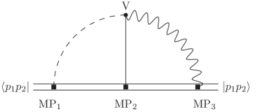
In the following we present the explicit calculation of the diagrams shown in Figure 1. The 5PN diagram on the r.h.s. is obtained as the closed Green’s function

$$I_{1} = {\mathbb{Z}}_{-}\Biggl{[}\tfrac{1}{3!}\prod_{l=1}^{3}\left[-i\int d^{D}w_{l}(V_{Qh}(w_{l})+V_{Qh^{2}}(w_{l})]\right]\tfrac{1}{2!}\prod_{k=1}^{2}\Biggl{[}-\frac{i}{2}\left(\int dy_{k}^{D}dz_{k}^{D}J_{-}(y_{k})\Delta_{\rm adv}(y_{k}-z_{k})\right.$$ (198)

$$\hskip 19.91684pt\left.\times J_{+}(z_{k})+J_{+}(y_{k})\Delta_{\rm ret}(y_{k}-z_{k})J_{-}(z_{k})+J_{+}(y_{k})\Delta_{\rm C}(y_{k}-z_{k})J_{+}(z_{k})\right)\Biggr{]}\Biggr{]},$$

i.e. integrating over the coordinates $x_{1}$ to $x_{3}$ and applying the ${\mathbb{Z}}_{-}$ operator, leading to

$$I_{1} = \Biggl{[}\frac{(-i)^{3}i^{4}}{3!}\int dx_{1}^{D}\int dx_{2}^{D}\int dx_{3}^{D}\Bigl{[}\delta_{J_{-}(x_{1})}Q_{+}(x_{1})V_{+}(x_{1})\delta_{J_{+}(x_{2})}^{2}Q_{-}(x_{2})V_{-}(x_{2})\delta_{J_{-}(x_{3})}Q_{+}(x_{3})V_{+}(x_{3})$$

$$\hskip 125.19194pt+\delta_{J_{+}(x_{1})}^{2}Q_{-}(x_{1})V_{-}(x_{1})\delta_{J_{-}(x_{2})}Q_{+}(x_{2})V_{+}(x_{2})\delta_{J_{-}(x_{3})}Q_{+}(x_{3})V_{+}(x_{3})$$

$$\hskip 125.19194pt+\delta_{J_{-}(x_{1})}Q_{+}(x_{1})V_{+}(x_{1})\delta_{J_{-}(x_{2})}Q_{+}(x_{2})V_{+}(x_{2})\delta_{J_{+}(x_{3})}^{2}Q_{-}(x_{3})V_{-}(x_{3})$$

$$\hskip 59.75095pt+2\big{[}\delta_{J_{-}(x_{1})}Q_{+}(x_{1})V_{+}(x_{1})\delta_{J_{-}(x_{2})}\delta_{J_{+}(x_{2})}Q_{+}(x_{2})V_{+}(x_{2})\delta_{J_{+}(x_{3})}Q_{-}(x_{3})V_{-}(x_{3})$$

$$\hskip 71.13188pt+\delta_{J_{-}(x_{1})}\delta_{J_{+}(x_{1})}Q_{+}(x_{1})V_{+}(x_{1})\delta_{J_{-}(x_{2})}Q_{+}(x_{2})V_{+}(x_{2})\delta_{J_{+}(x_{3})}Q_{-}(x_{3})V_{-}(x_{3})$$

$$\hskip 71.13188pt+\delta_{J_{+}(x_{1})}Q_{-}(x_{1})V_{-}(x_{1})\delta_{J_{-}(x_{2})}\delta_{J_{+}(x_{2})}Q_{+}(x_{2})V_{+}(x_{2})\delta_{J_{-}(x_{3})}Q_{+}(x_{3})V_{+}(x_{3})$$

$$\hskip 71.13188pt+\delta_{J_{-}(x_{1})}\delta_{J_{+}(x_{1})}Q_{+}(x_{1})V_{+}(x_{1})\delta_{J_{+}(x_{2})}Q_{-}(x_{2})V_{-}(x_{2})\delta_{J_{-}(x_{3})}Q_{+}(x_{3})V_{+}(x_{3})$$

$$\hskip 71.13188pt+\delta_{J_{-}(x_{1})}Q_{+}(x_{1})V_{+}(x_{1})\delta_{J_{+}(x_{2})}Q_{-}(x_{2})V_{-}(x_{2})\delta_{J_{-}(x_{3})}\delta_{J_{+}(x_{3})}Q_{+}(x_{3})V_{+}(x_{3})$$

$$\hskip 71.13188pt+\delta_{J_{+}(x_{1})}Q_{-}(x_{1})V_{-}(x_{1})\delta_{J_{-}(x_{2})}Q_{+}(x_{2})V_{+}(x_{2})\delta_{J_{-}(x_{3})}\delta_{J_{+}(x_{3})}Q_{+}(x_{3})V_{+}(x_{3})\big{]}\Bigr{]}$$

$$\leavevmode\nobreak\ \leavevmode\nobreak\ \leavevmode\nobreak\ \leavevmode\nobreak\ \times\tfrac{1}{2!}\prod_{k=4}^{5}\left[-\frac{i}{2}\left(\int dx_{k}^{D}dy_{k}^{D}J_{-}(x_{k})\Delta_{\rm adv}(x_{k}-y_{k})J_{+}(y_{k})\right.\right.$$

$$\left.\left.\leavevmode\nobreak\ \leavevmode\nobreak\ \leavevmode\nobreak\ +J_{+}(x_{k})\Delta_{\rm ret}(x_{k}-y_{k})J_{-}(y_{k})+J_{+}(x_{k})\Delta_{\rm C}(x_{k}-y_{k})J_{+}(y_{k})\right)\right]\Biggr{]}_{\rm conn.},$$

$$= -2\int dx_{1}^{D}\int dx_{2}^{D}\int dx_{3}^{D}\Delta_{\rm adv}(x_{1}-x_{2})Q_{+}(x_{1})V_{+}(x_{1})$$

$$\times\left[\Delta_{\rm adv}(x_{2}-x_{3})Q_{+}(x_{2})V_{+}(x_{2})Q_{-}(x_{3})V_{-}(x_{3})+\frac{\Delta_{\rm ret}(x_{2}-x_{3})}{2}Q_{-}(x_{2})V_{-}(x_{2})Q_{+}(x_{3})V_{+}(x_{3})\right].$$

Here $V_{\pm}(x_{i})$ denote the numerator functions at the respective vertices, while $G_{r(a)}(x_{i}-x_{j})$ are the retarded and advanced propagators in configuration space. In the diagrams of Figure 1 the propagator $\Delta_{\rm C}(x-y)$ does not contribute.

The Fourier transform from momentum to configuration space and its inverse are defined by [86, 87]

$${\bf F}[f](r) = \int\frac{d^{D}k}{(2\pi)^{D}}\exp[ik.r]f(k)$$ (201)

$${\bf F}^{-1}[g](k) = \int d^{D}r\exp[-ik.r]g(r).$$ (202)

One obtains the following contribution to the action in momentum space

$${\sf S}_{1} = {\frac{8}{3}\sqrt{2}\pi^{2}G_{N}^{2}}\int_{-\infty}^{+\infty}\frac{dl_{1}^{0}}{2\pi}\int_{-\infty}^{+\infty}\frac{dl_{2}^{0}}{2\pi}\int\frac{d^{d}{\bf l}_{1}}{(2\pi)^{d}}\int\frac{d^{d}{\bf l}_{2}}{(2\pi)^{d}}\frac{\tilde{Q}^{ij}_{+}(l_{1}^{0})}{|{\bf l}_{1}|^{2}-(l_{1}^{0}+i\delta)^{2}}$$ (203)

$$\times\Biggl{[}\frac{P_{11}[l_{1}^{0},l_{2}^{0}]\tilde{Q}^{jk}_{+}(-l_{1}^{0}-l_{2}^{0})\tilde{Q}^{ki}_{-}(l_{2}^{0})}{|{\bf l_{2}}|^{2}-(l_{2}^{0}+i\delta)^{2}}+\frac{1}{2}\frac{P_{12}[l_{1}^{0},l_{2}^{0}]\tilde{Q}^{jk}_{-}(-l_{1}^{0}-l_{2}^{0})\tilde{Q}^{ki}_{+}(l_{2}^{0})}{|{\bf l_{2}}|^{2}-(l_{2}^{0}-i\delta)^{2}}\Biggr{]},$$

with

$$-\int\frac{d^{d}{\mathbf{l}}_{1}}{(2\pi)^{d}}\frac{1}{|{\mathbf{l}}_{1}|^{2}-(l_{1}^{0}-i\delta)^{2}} = \frac{i}{4\pi}l_{1}^{0},$$ (204)

$$-\int\frac{d^{d}{\mathbf{l}}_{1}}{(2\pi)^{d}}\frac{1}{|{\mathbf{l}}_{1}|^{2}-(l_{1}^{0}+i\delta)^{2}} = -\frac{i}{4\pi}l_{1}^{0}\leavevmode\nobreak\$$ (205)

for $d=3$ represented by an analytic continuation in case [96]. Eq. (203) has been obtained after tensor decomposition and the use of master integrals, such that the three momenta appear only in the propagators.

We use

$$\tilde{Q}_{\pm}(k_{0})=\int_{-\infty}^{+\infty}dt\exp[-ik_{0}t]Q_{\pm}(t)$$ (206)

leading to

$${\sf S}_{1} = \frac{\sqrt{2}}{6}G_{N}^{2}\int_{-\infty}^{+\infty}\frac{dl_{1}^{0}}{2\pi}\int_{-\infty}^{+\infty}\frac{dl_{2}^{0}}{2\pi}l_{1}^{0}l_{2}^{0}\tilde{Q}_{+}(l_{1}^{0})$$ (207)

$$\times\Biggl{[}P_{11}[l_{1}^{0},l_{2}^{0}]\tilde{Q}_{+}(-l_{1}^{0}-l_{2}^{0})\tilde{Q}_{-}(l_{2}^{0})-\frac{1}{2}P_{12}[l_{1}^{0},l_{2}^{0}]\tilde{Q}_{-}(-l_{1}^{0}-l_{2}^{0})\tilde{Q}_{+}(l_{2}^{0})\Biggr{]},$$

with

$$P_{11}(x,y)=P_{12}(x,y)=x^{3}y^{3},$$ (208)

resulting in

$${\sf S}_{1}=\frac{\sqrt{2}}{12}G_{N}^{2}\int_{-\infty}^{+\infty}dt\leavevmode\nobreak\ {\rm tr}\left\{2Q_{+}(t)Q_{+}^{(4)}(t)Q_{-}^{(4)}(t)-Q_{-}(t)(Q_{+}^{(4)}(t))^{2}\right\}.$$ (209)

.

Let us also remark on the mathematical structure in the causal case for completeness, which does not contribute in the present case. Here the derivation of the final result requires a different technique. One has

$${\sf\tilde{S}}_{1}^{\rm c} = 8\pi^{2}G_{N}^{2}\int_{-\infty}^{+\infty}\frac{dl_{1}^{0}}{2\pi}\int_{-\infty}^{+\infty}\frac{dl_{2}^{0}}{2\pi}\int\frac{d^{D-1}{\mathbf{l}}_{1}}{(2\pi)^{D-1}}\int\frac{d^{D-1}{\mathbf{l}}_{2}}{(2\pi)^{D-1}}P_{2}[l_{1}^{0},l_{2}^{0}]\frac{\tilde{Q}(l_{1}^{0})\tilde{Q}(l_{2}^{0})\tilde{Q}(-l_{1}^{0}-l_{2}^{0})}{[(l_{1}^{0})^{2}-{\mathbf{l}}_{1}^{2}+i\delta][(l_{2}^{0})^{2}-{\mathbf{l}}_{2}^{2}+i\delta]}.$$

This integral leads to terms $\left((l_{k}^{0})^{2}+i\delta\right)^{1/2}$ which are Schwartz ${\mathcal{S}}^{\prime}$ distributions [86]. One has, cf. [87],

$$(z+i\delta)^{\lambda} = z_{+}^{\lambda}+\exp(+i\pi\lambda)z_{-}^{\lambda}$$ (211)

$$(z-i\delta)^{\lambda} = z_{+}^{\lambda}+\exp(-i\pi\lambda)z_{-}^{\lambda},$$ (212)

with $z,\lambda\in\mathbb{R}$ and $\lambda\neq 0,-1,-2,-3,...$ and

$$z_{+}^{\lambda} = \theta(+z)z^{\lambda}$$ (213)

$$z_{-}^{\lambda} = \theta(-z)(-z)^{\lambda}.$$ (214)

Due to the polynomial $P_{2}$ in (D) we have to consider Fourier-transforms of $f\in{\cal S}^{\prime}$ distributions of the kind

$${\bf F}^{-1}[x^{m}f(x)](\sigma)=(-i)^{m}\frac{\partial^{m}}{\partial\sigma^{m}}{\bf F}^{-1}[f(x)](\sigma),\leavevmode\nobreak\ \leavevmode\nobreak\ \leavevmode\nobreak\ m\in\mathbb{N}.$$ (215)

Since $(l_{1}^{0})^{2}>0$ one has

$$\left((l_{1}^{0})^{2}+i\delta\right)^{1/2}=\left[\sqrt{(l_{1}^{0})^{2}}\right]_{+}=|l_{1}^{0}|.$$ (216)

We consider now the one-dimensional Fourier transform of the distribution $z_{\pm}^{\lambda}$, cf. [87].

$${\bf F}^{-1}[z_{+}^{\lambda}](t) = i\frac{\Gamma(\lambda+1)}{2\pi}\frac{\exp[i\lambda\pi/2]}{(-t+i\delta)^{\lambda+1}},$$ (217)

$${\bf F}^{-1}[z_{-}^{\lambda}](t) = -i\frac{\Gamma(\lambda+1)}{2\pi}\frac{\exp[-i\lambda\pi/2]}{(-t-i\delta)^{\lambda+1}}$$ (218)

and one has

$${\bf F}^{-1}[|z|](t) = {\bf F}^{-1}[z_{+}](t)+{\bf F}^{-1}[z_{-}](t)=-\frac{1}{2\pi}\Biggl{[}\frac{1}{(t+i\delta)^{2}}+\frac{1}{(t-i\delta)^{2}}\Biggr{]}.$$ (219)

Only the first term in the r.h.s. contributes to the contour integral using the residue theorem.

As an example we consider

$$P_{2}(l_{1}^{0},l_{2}^{0})=(l_{1}^{0})^{2}(l_{2}^{0})^{2}[l_{1}^{0}+l_{2}^{0}]^{2}.$$ (220)

According to (215) the polynomial implies the term

$$-\frac{1}{4\pi^{2}}\Biggl{[}\frac{1440}{(t_{1}-t+i\delta)^{6}(t_{2}-t+i\delta)^{4}}+\frac{1152}{(t_{1}-t+i\delta)^{5}(t_{2}-t+i\delta)^{5}}\Biggr{]}.$$ (221)

Therefore we have

$${\sf\tilde{S}}_{1}^{\rm c} = 8\pi^{2}G_{N}^{2}\int_{-\infty}^{+\infty}dtQ(t)\int_{-\infty}^{+\infty}dt_{1}\int_{-\infty}^{+\infty}dt_{2}\frac{(-1)}{16\pi^{2}}\frac{(-1)}{4\pi^{2}}$$

$$\times\Biggl{\{}\frac{1440}{(t_{1}-t+i\delta)^{6}(t_{2}-t+i\delta)^{4}}+\frac{1152}{(t_{1}-t+i\delta)^{5}(t_{2}-t+i\delta)^{5}}\Biggr{\}}Q(t_{1})Q(t_{2})$$

$$= {-}16\pi^{2}G_{N}^{2}\frac{(-1)^{2}}{64\pi^{4}}(2\pi i)^{2}\int_{-\infty}^{+\infty}dtQ(t)\Biggl{\{}\left[\frac{d^{5}}{dt^{5}}Q(t)\right]\left[\frac{d^{3}}{dt^{3}}Q(t)\right]+\left[\frac{d^{4}}{dt^{4}}Q(t)\right]^{2}\Biggr{\}}$$

$$= G_{N}^{2}\int_{-\infty}^{+\infty}dtQ(t)\Biggl{\{}\left[\frac{d^{5}}{dt^{5}}Q(t)\right]\left[\frac{d^{3}}{dt^{3}}Q(t)\right]+\left[\frac{d^{4}}{dt^{4}}Q(t)\right]^{2}\Biggr{\}}$$ (223)

$$= \frac{G_{N}^{2}}{2}\int_{-\infty}^{+\infty}dt\left[\frac{d^{2}}{dt^{2}}Q(t)\right]\left[\frac{d^{3}}{dt^{3}}Q(t)\right]^{2},$$ (224)

using the residue theorem, [97], since $Q(t)$ is bounded and obeys a Taylor expansion. The result is given in (223). In (224) it has been further assumed, that $Q(t)$ and the derivatives of $Q(t)$ vanish in the limit $t\rightarrow\pm\infty$. (224) is again a Riemann integral.

We finally turn to the memory term, Figure 1 r.h.s. The corresponding Green’s function is obtained by carrying out the functional derivations in $I_{2}$

$$I_{2}\leavevmode\nobreak\ = \leavevmode\nobreak\ \biggl{[}\frac{i^{10}}{3!}\int dx^{D}_{1}\int dx^{D}_{2}\int dx^{D}_{3}\int dx^{D}_{4}\ \Bigl{[}\delta_{J_{-}(x_{1})}Q_{+}(x_{1})V_{+}(x_{1})\delta_{J_{-}(x_{2})}Q_{+}(x_{2})V_{+}(x_{2})$$ (225)

$$\times\delta_{J_{+}(x_{3})}Q_{-}(x_{3})V_{-}(x_{3})$$

$$+\delta_{J_{-}(x_{1})}Q_{+}(x_{1})V_{+}(x_{1})\delta_{J_{+}(x_{2})}Q_{-}(x_{2})V_{-}(x_{2})\delta_{J_{-}(x_{3})}Q_{+}(x_{3})V_{+}(x_{3})$$

$$+\delta_{J_{+}(x_{1})}Q_{-}(x_{1})V_{-}(x_{1})\delta_{J_{-}(x_{2})}Q_{+}(x_{2})V_{+}(x_{2})\delta_{J_{-}(x_{3})}Q_{+}(x_{3})V_{+}(x_{3})\Bigr{]}\delta_{J_{+}(x_{4})}^{2}\delta_{J_{-}(x_{4})}v(x_{4})$$

$$\times\frac{1}{3!}\prod_{k=5}^{8}\biggl{[}-\frac{i}{2}\int dx_{k}^{D}dy_{k}^{D}\ (J_{-}(x_{k})\Delta_{\text{adv}}(x_{k}-y_{k})J_{+}(y_{k})$$

$$+J_{+}(x_{k})\Delta_{\text{ret}}(x_{k}-y_{k})J_{-}(y_{k})+J_{+}(x_{k})\Delta_{\text{C}}(x_{k}-y_{k})J_{+}(y_{k}))\biggr{]}\biggr{]}_{\text{conn.}}$$

and setting the Schwinger parameters to zero. Here the function $v$ refers to the contributing triple bulk vertices, including their combinatorics, and also account for the propagator numerators as also $V_{\pm}$ at the multipole vertices. Unlike the case for $I_{1}$, here various fields are contributing. By analogous operations as in the case of ${\sf S}_{1}$ one obtains

$${\sf{S}}_{2} = {-}G_{N}^{2}\sqrt{2}\frac{1}{10}\int_{-\infty}^{+\infty}dt\leavevmode\nobreak\ {\rm tr}\Bigl{\{}\frac{4}{7}\left[3Q_{+}^{(2)}(t)Q_{+}^{(3)}(t)Q_{-}^{(3)}(t)-2Q_{-}^{(2)}(t)Q_{+}^{(3)}(t)Q_{+}^{(3)}(t)\right]$$ (226)

$$+\left[2Q_{+}(t)Q_{+}^{(4)}(t)Q_{-}^{(4)}(t)-Q_{-}(t)Q_{+}^{(4)}(t)Q_{+}^{(4)}(t)\right]\Bigr{\}}.$$

Finally one obtains from these terms the contributions (2–2).

To extract the conservative part of the action, we express $\textsf{S}_{1}$ and $\textsf{S}_{2}$ in terms of $Q_{1},Q_{2}$:

$$\textsf{S}_{i}={} \int dt\ \bigl{(}L_{i}[Q_{1}]-L_{i}[Q_{2}]+R_{i}[Q_{1},Q_{2}]\bigr{)}\qquad i=1,2,$$ (227)

$$L_{1}[Q_{j}]={} \frac{G_{N}^{2}}{24}\operatorname{tr}\left[Q_{j}Q_{j}^{(4)}Q_{j}^{(4)}\right],$$ (228)

$$L_{2}[Q_{j}]={} {-}G_{N}^{2}\operatorname{tr}\left[\frac{1}{20}Q_{j}Q_{j}^{(4)}Q_{j}^{(4)}+\frac{1}{35}Q_{j}^{(2)}Q_{j}^{(3)}Q_{j}^{(3)}\right],$$ (229)

$$R_{1}[Q_{1},Q_{2}]={} G_{N}^{2}\operatorname{tr}\left[{-}\frac{1}{12}Q_{1}Q_{1}^{(4)}Q_{2}^{(4)}{+}\frac{1}{8}Q_{2}Q_{1}^{(4)}Q_{1}^{(4)}\right]-(1\leftrightarrow 2),$$ (230)

$$R_{2}[Q_{1},Q_{2}]={} G_{N}^{2}\operatorname{tr}\left[\frac{1}{10}Q_{1}Q_{1}^{(4)}Q_{2}^{(4)}{-}\frac{3}{20}Q_{2}Q_{1}^{(4)}Q_{1}^{(4)}{+}\frac{4}{35}Q_{1}^{(2)}Q_{1}^{(3)}Q_{2}^{(3)}{-}\frac{1}{7}Q_{2}^{(2)}Q_{1}^{(3)}Q_{1}^{(3)}\right]$$

$$-(1\leftrightarrow 2),$$ (231)

cf. (162). Following [62], we identify $L_{1}$ and $L_{2}$ with the conservative contribution to the Lagrangian. We therefore add $L_{1}[Q]+L_{2}[Q]$ to the Lagrangian derived in [16] by integrating out the potential modes. After eliminating accelerations and higher time derivatives as outlined in [16], we perform a Legendre transformation to obtain a Hamiltonian. The contribution resulting from $\textsf{S}_{1}$ is given by equation (2). For $\textsf{S}_{2}$, the first term in equation (229) gives rise to equation (2) and the second term to equation (2).

Appendix E Scattering angle integrals

In the following we list integrals, which appear in the calculation of the scattering angle, using relations given in [74].

At the Newtonian level one obtains the well–known integral

$$I_{0} = \int_{0}^{x_{\rm max}}{dx}\frac{1}{\displaystyle\sqrt{1-x^{2}+\frac{2x}{jp_{\infty}}}}=-\frac{\pi}{2}+{\rm arcsin}\left(\frac{1}{\sqrt{1+j^{2}p_{\infty}^{2}}}\right).$$ (232)

It implies the value $\pi/2$ in (48). Its $\eta$–expansion delivers the $\nu$ and $\eta$–independent terms of $\chi_{2k+1}$ with

$$I_{0}^{\rm(reg)} = -\frac{\pi}{2}+\frac{1}{p_{\infty}j}-\frac{1}{3p_{\infty}^{3}j^{3}}+\frac{1}{5p_{\infty}^{5}j^{5}}+O\left(\frac{1}{j^{7}}\right).$$ (233)

The $O(\eta^{2})$ term reads

$$I_{2} = \eta^{2}\Biggl{[}\frac{2p_{\infty}}{j}+\frac{3\pi}{2j^{2}}+\frac{4}{j^{3}p_{\infty}}-\frac{2}{j^{5}p_{\infty}^{3}}-\frac{10}{7j^{9}p_{\infty}^{7}}+\frac{8}{5j^{7}p_{\infty}^{5}}+\frac{4}{3j^{11}p_{\infty}^{9}}\Biggr{]}+O\left(\frac{1}{p_{\infty}^{11}}\right)+O\left(\frac{1}{\sqrt{\varepsilon}}\right).$$

The $O(\eta^{4})$ is given by

$$I_{4} = \eta^{4}\Biggl{[}\pi\left(\frac{15}{8}-\frac{3}{4}\nu\right)p_{\infty}^{2}\frac{1}{j^{2}}+(24-8\nu)p_{\infty}\frac{1}{j^{3}}+\pi\left(\frac{105}{8}-\frac{15}{4}\nu\right)\frac{1}{j^{4}}+(32-8\nu)\frac{1}{j^{5}p_{\infty}}$$

$$-\left(16-\frac{16}{5}\nu\right)\frac{1}{j^{7}p_{\infty}^{3}}+\left(\frac{96}{7}-\frac{16}{7}\nu\right)\frac{1}{j^{9}p_{\infty}^{5}}-\left(\frac{40}{3}-\frac{40}{21}\nu\right)\frac{1}{j^{11}p_{\infty}^{7}}\Biggr{]}+O\left(\frac{1}{p_{\infty}^{9}}\right)+O\left(\frac{1}{\varepsilon^{3/2}}\right).$$

Similar structures are obtained for the higher order terms in $\eta$. Here the singularity in $\varepsilon$ becomes stronger by one unit going from $I_{2k}$ to $I_{2k+2}$. One easily sees that these integrals form the first terms of the coefficients $\chi_{k}$ given in Eq. (87–92).

We also list a series of higher expansion coefficients for $\chi^{\rm Schw}_{k}$ for convenience, which result from (3.2),

$$\chi^{\rm Schw}_{5} = \frac{1}{5p_{\infty}}-\frac{2\eta^{2}}{p_{\infty}^{3}}+\frac{32\eta^{4}}{p_{\infty}}+320p_{\infty}\eta^{6}+640p_{\infty}^{3}\eta^{8}+\frac{1792}{5}p_{\infty}^{5}\eta^{10},$$ (236)

$$\chi^{\rm Schw}_{6} = \pi\left(\frac{1155}{8}\eta^{6}+\frac{45045}{64}p_{\infty}^{2}\eta^{8}+\frac{135135}{128}p_{\infty}^{4}\eta^{10}+\frac{255255}{512}p_{\infty}^{6}\eta^{12}\right),$$ (237)

$$\chi^{\rm Schw}_{7} = -\frac{1}{7p_{\infty}^{7}}+\frac{8\eta^{2}}{5p_{\infty}^{5}}-\frac{16\eta^{4}}{p_{\infty}^{3}}+\frac{320\eta^{6}}{p_{\infty}}+4480p_{\infty}\eta^{8}+14336p_{\infty}^{3}\eta^{10}+\frac{86016}{5}p_{\infty}^{5}\eta^{12}+\frac{49152}{7}p_{\infty}^{7}\eta^{14},$$

$$\chi^{\rm Schw}_{8} = \pi\left(\frac{225225}{128}\eta^{8}+\frac{765765}{64}p_{\infty}^{2}\eta^{10}+\frac{14549535}{512}p_{\infty}^{4}\eta^{12}+\frac{14549535}{512}p_{\infty}^{6}\eta^{14}+\frac{334639305}{32768}p_{\infty}^{8}\eta^{16}\right),$$

$$\chi^{\rm Schw}_{9} = \frac{1}{9p_{\infty}^{9}}-\frac{10\eta^{2}}{7p_{\infty}^{7}}+\frac{96\eta^{4}}{7p_{\infty}^{5}}-\frac{448\eta^{6}}{3p_{\infty}^{3}}+\frac{3584\eta^{8}}{p_{\infty}}+64512p_{\infty}\eta^{10}+286720p_{\infty}^{3}\eta^{12}+540672p_{\infty}^{5}\eta^{14}$$ (240)

$$+\frac{3244032}{7}p_{\infty}^{7}\eta^{16}+\frac{9371648}{63}p_{\infty}^{9}\eta^{18},$$

$$\chi^{\rm Schw}_{10} = \pi\left(\frac{2909907}{128}\eta^{10}+\frac{101846745}{512}p_{\infty}^{2}\eta^{12}+\frac{334639305}{512}p_{\infty}^{4}\eta^{14}+\frac{8365982625}{8192}p_{\infty}^{6}\eta^{16}\right.$$ (241)

$$\left.+\frac{25097947875}{32768}p_{\infty}^{8}\eta^{18}+\frac{29113619535}{131072}p_{\infty}^{10}\eta^{20}\right),$$

$$\chi^{\rm Schw}_{11} = -\frac{1}{11p_{\infty}^{11}}+\frac{4\eta^{2}}{3p_{\infty}^{9}}-\frac{40\eta^{4}}{3p_{\infty}^{7}}+\frac{128\eta^{6}}{p_{\infty}^{5}}-\frac{1536\eta^{8}}{p_{\infty}^{3}}+\frac{43008\eta^{10}}{p_{\infty}}+946176p_{\infty}\eta^{12}+5406720p_{\infty}^{3}\eta^{14}$$ (242)

$$+14057472p_{\infty}^{5}\eta^{16}+18743296p_{\infty}^{7}\eta^{18}+\frac{37486592p_{\infty}^{9}}{3}\eta^{20}+\frac{109051904p_{\infty}^{11}}{33}\eta^{22},$$

$$\chi^{\rm Schw}_{12} = \pi\left(\frac{156165009}{512}\eta^{12}+\frac{1673196525}{512}p_{\infty}^{2}\eta^{14}+\frac{225881530875}{16384}p_{\infty}^{4}\eta^{16}+\frac{242613496125}{8192}p_{\infty}^{6}\eta^{18}\right.$$ (243)

$$\left.+\frac{4512611027925}{131072}p_{\infty}^{8}\eta^{20}+\frac{2707566616755}{131072}p_{\infty}^{10}\eta^{22}+\frac{10529425731825}{2097152}p_{\infty}^{12}\eta^{24}\right),$$

$$\chi^{\rm Schw}_{13} = \frac{1}{13p_{\infty}^{13}}-\frac{14\eta^{2}}{11p_{\infty}^{11}}+\frac{448\eta^{4}}{33p_{\infty}^{9}}-\frac{128\eta^{6}}{p_{\infty}^{7}}+\frac{1280\eta^{8}}{p_{\infty}^{5}}-\frac{16896\eta^{10}}{p_{\infty}^{3}}+\frac{540672\eta^{12}}{p_{\infty}}+14057472p_{\infty}\eta^{14}$$ (244)

$$+98402304p_{\infty}^{3}\eta^{16}+328007680p_{\infty}^{5}\eta^{18}+599785472p_{\infty}^{7}\eta^{20}+\frac{1853882368p_{\infty}^{9}}{3}\eta^{22}$$

$$+\frac{3707764736p_{\infty}^{11}}{11}\eta^{24}+\frac{10838081536p_{\infty}^{13}}{143}\eta^{26},$$

$$\chi^{\rm Schw}_{14} = \pi\left(\frac{2151252675}{512}\eta^{14}+\frac{436704293025p_{\infty}^{2}}{8192}\eta^{16}+\frac{4512611027925p_{\infty}^{4}}{16384}\eta^{18}\right.$$ (245)

$$\left.+\frac{49638721307175p_{\infty}^{6}}{65536}\eta^{20}+\frac{157941385977375p_{\infty}^{8}}{131072}\eta^{22}+\frac{1168766256232575p_{\infty}^{10}}{1048576}\eta^{24}\right.$$

$$\left.+\frac{1168766256232575p_{\infty}^{12}}{2097152}\eta^{26}+\frac{977947275623175p_{\infty}^{14}}{8388608}\eta^{28}\right).$$

Acknowledgment. We thank Th. Damour, S. Foffa, R. Sturani, Z. Bern, M. Ruf, G. Kaelin, L. Blanchet, C. Kavanagh, and B. Wardell for discussions. This work has been funded in part by EU TMR network SAGEX agreement No. 764850 (Marie Skłodowska–Curie). G. Schäfer has been supported in part by Kolleg Mathematik Physik Berlin (KMPB) and DESY. The Feynman-type diagrams shown have been drawn using axodraw, [98] and Asymptote [99].

Note added. After completion of this paper two preprints appeared [100], in which the representation of the electric quadrupole moment have been given in $d$ dimensions, without the previously used additional Hadamard regularization [101]. This new representation has no impact on the results of the present calculation.

S. Foffa communicated to us a note in preparation [102], in which it is shown that the previously necessary finite renormalization of the magnetic quadrupole term JEJ, using a representation containing Levi-Civita symbols, can be avoided by utilizing a dual representation, free of them, giving the same result.

After submission of the present paper, Ref. [68] appeared, confirming Eq. (6.17) of [42] in the post-Minkowskian approach to $O(G_{N}^{4}/r^{4})$. The tail terms resulting from the multipole–expansion alone, within the Hamiltonian approach to the bound state problem, however, do not lead to this result, as has been shown by the explicit calculation in the present paper in detail. Ref. [68] compares to Ref. [42] not in the scattering angle defined in [15] but in the quantity ${\cal M}_{4}^{\rm radgrav,f}$. We mention that, on the other hand, the potential terms do fully agree between Refs. [76] and [77].

For future work it would be highly desirable to have a consistent field theoretic description of the tail terms ab initio with Feynman rules to all orders in the effective field theory approach. First steps in this direction have been undertaken in Ref. [16] already, by using expansion by regions, cf. [103] for a survey.

Very recently a phenomenological analysis on the impact of the numerical difference described in Section 3.2 on the scattering angle has been made in Ref. [104], coming to the result of an effect of $10^{-3}$ in $120$ and larger. Here velocities of $v\leq 1/2$ have been assumed. Despite of this, however, we will aim at the determination of the exact analytic result in the future.

References

• [1] B.P. Abbott et al. (Virgo, LIGO Scientific), Phys. Rev. Lett. 116 (2016) 061102 [arXiv:1602.03837 [gr-qc]]; Phys. Rev. X 6 (2016) 041015 [arXiv:1606.04856 [gr-qc]]; Phys. Rev. Lett. 119 (2017) 161101 (2017), [arXiv:1710.05832 [gr-qc]]; Phys. Rev. X 9 (2019) 031040 [arXiv:1811.12907 [astro-ph.HE]].
• [2] Y. Aso, Y. Michimura, K. Somiya, M. Ando, O. Miyakawa, T. Sekiguchi, D. Tatsumi, and H. Yamamoto (KAGRA), Phys. Rev. D 88 (2013) 043007 [arXiv:1306.6747 [gr-qc]];
F. Acernese et al. (VIRGO), Class. Quant. Grav. 32 (2015) 024001 [arXiv:1408.3978 [gr-qc]];
J. Aasi et al. (LIGO Scientific), Class. Quant. Grav. 32 (2015) 074001 [arXiv:1411.4547 [gr-qc]];
B. Iyer et al. (LIGO Collaboration), LIGO-India, Proposal of the Consortium for Indian Initiative in Gravitational-wave Observations (2011), LIGO Document M1100296-v2.
• [3] A. Einstein, Sitzungsber. Preuss. Akad. Wiss. (1915) 831–839;
J. Droste, Proc. Acad. Sci. Amst. 19 (1916) 447–455;
H. Lorentz and J. Droste, in: The motion of a system of bodies under the influence of their mutual attraction, according to Einstein’s theory, (Nijhoff, The Hague, 1937) pp. 330–355;
A. Einstein, L. Infeld and B. Hoffmann, Annals Math.  39 (1938) 65–100;
H.P. Robertson, Annals Math. 39 (1938) 101–104;
A. Eddington and G.L. Clark, Proc. R. Soc. London A 166 (1938) 465–475.
• [4] B. Kol and M. Smolkin, Class. Quant. Grav. 25 (2008) 145011 [arXiv:0712.4116 [hep-th]].
• [5] S. Chandrasekhar, Astrophys. J.  142 (1965) 1488–1512;
Astrophys. J. 158 (1969) 45–54;
S. Chandrasekhar and Y. Nutku, Astrophys. J. 158 (1969) 55–79;
S. Chandrasekhar and F. Esposito, Astrophys. J. 160 (1970) 153–179;
C. Hoenselaers, Prog. Theor. Phys. 56 (1976) 324–326;
T. Damour and G. Schäfer, C.R. Acad. Sci. Paris 305, série II, (1987) 839–842; Nuovo Cim. B 101 (1988) 127–176;
T. Ohta and T. Kimura, Prog. Theor. Phys. 81 (1989) 679–689;
G. Schäfer and N. Wex, Phys. Lett. A 174 (1993) 196–205;
T. Ohta, H. Okamura, K. Hiida and T. Kimura, Prog. Theor. Phys. 50 (1973) 492–514; 51 (1974) 1598–1612; 51 (1974) 1220–1238;
T. Damour and N. Deruelle, C. R. Acad. Sci. série II 293 (1981) 537–540;
T. Damour, C.R. Acad. Sci. série II 294 (1982) 1355–1357; and in: Gravitational Radiation, eds. N. Deruelle and T. Piran (NATO ASI, North-Holland, Amsterdam, 1983) 59–144;
T. Damour and G. Schäfer, Gen. Rel. Grav. 17 (1985) 879–905;
S.M. Kopeikin, Sov. Astron. 29 (1985) 516–524;
L.P. Grishchuk and S.M. Kopeikin, in: Relativity in Celestial Mechanics and Astrometry: High Precision Dynamical Theories and Observational Verifications, eds. J. Kovalevsky and V. A. Brumberg (D. Reidel Publishing, Dordrecht, 1986) 19–34;
M.E. Pati and C.M. Will, Phys. Rev. D 65 (2002) 104008 [arXiv:gr-qc/0201001 [gr-qc]];
J.B. Gilmore and A. Ross, Phys. Rev. D 78 (2008) 124021 [arXiv:0810.1328 [gr-qc]].
• [6] P. Jaranowski and G. Schäfer, Phys. Rev. D 57 (1998) 7274–7291 [Erratum: Phys. Rev. D 63 (2001) 029902] [arXiv:gr-qc/9712075 [gr-qc]]; Phys. Rev. D 60 (1999) 124003 [arXiv:gr-qc/9906092 [gr-qc]];
T. Damour, P. Jaranowski and G. Schäfer, Phys. Rev. D 62 (2000) 044024 [arXiv:gr-qc/9912092 [gr-qc]]; Phys. Rev. D 62 (2000) 021501 [Erratum: Phys. Rev. D 63 (2001), 029903] [arXiv:gr-qc/0003051 [gr-qc]]; Phys. Lett. B 513 (2001) 147–155 [arXiv:gr-qc/0105038 [gr-qc]];
L. Blanchet and G. Faye, Phys. Lett. A 271 (2000) 58–64 [arXiv:gr-qc/0004009 [gr-qc]];
V.C. de Andrade, L. Blanchet and G. Faye, Class. Quant. Grav. 18 (2001) 753–778 [arXiv:gr-qc/0011063 [gr-qc]];
L. Blanchet, T. Damour and G. Esposito-Farese, Phys. Rev. D 69 (2004) 124007 [arXiv:gr-qc/0311052 [gr-qc]];
Y. Itoh and T. Futamase, Phys. Rev. D 68 (2003) 121501 [arXiv:gr-qc/0310028 [gr-qc]];
Y. Itoh, Phys. Rev. D 69 (2004) 064018 [arXiv:gr-qc/0310029 [gr-qc]];
R.M. Memmesheimer, A. Gopakumar and G. Schäfer, Phys. Rev. D 70 (2004) 104011 [arXiv:gr-qc/0407049 [gr-qc]];
S. Foffa and R. Sturani, Phys. Rev. D 84 (2011) 044031 [arXiv:1104.1122 [gr-qc]].
• [7] T. Damour, P. Jaranowski and G. Schäfer, Phys. Rev. D 89 (2014) no.6, 064058 [arXiv:1401.4548 [gr-qc]].
• [8] P. Jaranowski and G. Schäfer, Phys. Rev. D 92 (2015) no.12, 124043 [arXiv:1508.01016 [gr-qc]];
L. Bernard, L. Blanchet, A. Bohé, G. Faye and S. Marsat, Phys. Rev. D 93 (2016) no.8, 084037 [arXiv:1512.02876 [gr-qc]];
T. Damour, P. Jaranowski and G. Schäfer, Phys. Rev. D 93 (2016) no.8, 084014 [arXiv:1601.01283 [gr-qc]];
T. Damour and P. Jaranowski, Phys. Rev. D 95 (2017) no.8, 084005 [arXiv:1701.02645 [gr-qc]];
S. Foffa, P. Mastrolia, R. Sturani and C. Sturm, Phys. Rev. D 95 (2017) no.10, 104009 [arXiv:1612.00482 [gr-qc]];
L. Bernard, L. Blanchet, A. Bohé, G. Faye and S. Marsat, Phys. Rev. D 95 (2017) no.4, 044026 [arXiv:1610.07934 [gr-qc]];
T. Marchand, L. Bernard, L. Blanchet and G. Faye, Phys. Rev. D 97 (2018) no.4, 044023 [arXiv:1707.09289 [gr-qc]];
L. Bernard, L. Blanchet, G. Faye and T. Marchand, Phys. Rev. D 97 (2018) no.4, 044037 [arXiv:1711.00283 [gr-qc]].
• [9] S. Foffa and R. Sturani, Phys. Rev. D 100 (2019) no.2, 024047 [arXiv:1903.05113 [gr-qc]].
• [10] S. Foffa, R.A. Porto, I. Rothstein and R. Sturani, Phys. Rev. D 100 (2019) no.2, 024048 [arXiv:1903.05118 [gr-qc]].
• [11] J. Blümlein, A. Maier, P. Marquard and G. Schäfer, Nucl. Phys. B 955 (2020) 115041 [arXiv:2003.01692 [gr-qc]].
• [12] S. Foffa, P. Mastrolia, R. Sturani, C. Sturm and W.J. Torres Bobadilla, Phys. Rev. Lett.  122 (2019) no.24, 241605 [arXiv:1902.10571 [gr-qc]].
• [13] J. Blümlein, A. Maier and P. Marquard, Phys. Lett. B 800 (2020) 135100 [arXiv:1902.11180 [gr-qc]].
• [14] D. Bini, T. Damour and A. Geralico, Phys. Rev. Lett.  123 (2019) no.23, 231104 [arXiv:1909.02375 [gr-qc]].
• [15] D. Bini, T. Damour and A. Geralico, Phys. Rev. D 102 (2020) no.2, 024062 [arXiv:2003.11891 [gr-qc]].
• [16] J. Blümlein, A. Maier, P. Marquard and G. Schäfer, Nucl. Phys. B 965 (2021) 115352 [arXiv:2010.13672 [gr-qc]].
• [17] S. Foffa, R. Sturani and W. J. Torres Bobadilla, JHEP 02 (2021) 165 [arXiv:2010.13730 [gr-qc]].
• [18] D. Bini, T. Damour and A. Geralico, Phys. Rev. D 102 (2020) no.2, 024061 [arXiv:2004.05407 [gr-qc]].
• [19] D. Bini, T. Damour and A. Geralico, Phys. Rev. D 102 (2020) no.8, 084047 [arXiv:2007.11239 [gr-qc]].
• [20] J. Blümlein, A. Maier, P. Marquard and G. Schäfer, Phys. Lett. B 807 (2020), 135496 [arXiv:2003.07145 [gr-qc]].
• [21] J. Blümlein, A. Maier, P. Marquard, G. Schäfer and C. Schneider, Phys. Lett. B 801 (2020) 135157 [arXiv:1911.04411 [gr-qc]];
M. Accettulli Huber, A. Brandhuber, S. De Angelis and G. Travaglini, Phys. Rev. D 102 (2020) no.4, 046014 [arXiv:2006.02375 [hep-th]];
G. Kälin, Z. Liu and R.A. Porto, Phys. Rev. Lett. 125 (2020) no.26, 261103 [arXiv:2007.04977 [hep-th]];
G. Kälin and R.A. Porto, JHEP 11 (2020), 106 [arXiv:2006.01184 [hep-th]]; G. Kälin and R.A. Porto, JHEP 01 (2020) 072 [arXiv:1910.03008 [hep-th]];
T. Damour, Phys. Rev. D 102 (2020) no.12, 124008 [arXiv:2010.01641 [gr-qc]].
• [22] G. Kälin and R. A. Porto, JHEP 02 (2020) 120 [arXiv:1911.09130 [hep-th]].
• [23] T. Damour, Phys. Rev. D 102 (2020) no.2, 024060 [arXiv:1912.02139 [gr-qc]].
• [24] Z. Bern, C. Cheung, R. Roiban, C.H. Shen, M.P. Solon and M. Zeng, Phys. Rev. Lett.  122 (2019) no.20, 201603 [arXiv:1901.04424 [hep-th]];
Z. Bern, C. Cheung, R. Roiban, C.H. Shen, M.P. Solon and M. Zeng, JHEP 1910 (2019) 206 [arXiv:1908.01493 [hep-th]];
• [25] D. Bini and T. Damour, Phys. Rev. D 89 (2014) no.10, 104047 [arXiv:1403.2366 [gr-qc]]; Phys. Rev. D 91 (2015), 064050 [arXiv:1502.02450 [gr-qc]];
C. Kavanagh, A.C. Ottewill and B. Wardell, Phys. Rev. D 92 (2015) no.8, 084025 [arXiv:1503.02334 [gr-qc]].
• [26] Electronic archive of post-newtonian coefficients,
http://www.barrywardell.net/research/code
• [27] L. Blanchet, S. Foffa, F. Larrouturou and R. Sturani, Phys. Rev. D 101 (2020) no.8, 084045 [arXiv:1912.12359 [gr-qc]].
• [28] S.L. Detweiler, Phys. Rev. D 77 (2008) 124026 [arXiv:0804.3529 [gr-qc]];
L. Barack and N. Sago, Phys. Rev. Lett. 102 (2009) 191101 [arXiv:0902.0573 [gr-qc]];
T. Damour, Phys. Rev. D 81 (2010) 024017 [arXiv:0910.5533 [gr-qc]];
L. Blanchet, S.L. Detweiler, A. Le Tiec and B.F. Whiting, Phys. Rev. D 81 (2010), 084033 [arXiv:1002.0726 [gr-qc]];
L. Barack and A. Pound, Rept. Prog. Phys. 82 (2019) no.1, 016904 [arXiv:1805.10385 [gr-qc]].
• [29] W.D. Goldberger and I.Z. Rothstein, Phys. Rev. D 73 (2006) 104029 [hep-th/0409156].
• [30] S. Foffa and R. Sturani, Phys. Rev. D 101 (2020) no.6, 064033 [Erratum: Phys. Rev. D 103 (2021) no.8, 089901] [arXiv:1907.02869v5 [gr-qc]].
• [31] P. Nogueira, J. Comput. Phys.  105 (1993) 279–289.
• [32] J.A.M. Vermaseren, New features of FORM, math-ph/0010025;
M. Tentyukov and J.A.M. Vermaseren, Comput. Phys. Commun.  181 (2010) 1419–1427 [hep-ph/0702279].
• [33] P. Marquard and D. Seidel, The Crusher algorithm, unpublished.
• [34] J. Lagrange, Nouvelles recherches sur la nature et la propagation du son, Miscellanea Taurinensis, t. II, 1760-61; Oeuvres t. I, p. 263;
C.F. Gauß, Theoria attractionis corporum sphaeroidicorum ellipticorum homogeneorum methodo novo tractate, Commentationes societas scientiarum Gottingensis recentiores, Vol III, 1813, Werke Bd. V pp. 5–7;
G. Green, Essay on the Mathematical Theory of Electricity and Magnetism, Nottingham, 1828 [Green Papers, pp. 1–115];
M. Ostrogradski, Mem. Ac. Sci. St. Peters., 6, (1831) 39–53;
K.G. Chetyrkin and F.V. Tkachov, Nucl. Phys. B 192 (1981) 159–204;
S. Laporta, Int. J. Mod. Phys. A 15 (2000) 5087–5159 [hep-ph/0102033].
• [35] K.S. Thorne, Rev. Mod. Phys. 52 (1980) 299–339.
• [36] L. Blanchet and T. Damour, Phil. Trans. Roy. Soc. Lond. A 320 (1986) 379–430;
L. Blanchet and T. Damour, Phys. Rev. D 37 (1988) 1410–1435;
L. Blanchet and G. Schäfer, Class. Quant. Grav. 10 (1993) 2699–2721;
O. Poujade and L. Blanchet, Phys. Rev. D 65 (2002) 124020 [arXiv:gr-qc/0112057 [gr-qc]];
W.D. Goldberger and I.Z. Rothstein, Phys. Rev. D 73 (2006) 104030 [arXiv:hep-th/0511133 [hep-th]];
G.L. Almeida, S. Foffa and R. Sturani, JHEP 11 (2020), 165 [arXiv:2008.06195 [gr-qc]].
• [37] A. Ross, Phys. Rev. D 85 (2012) 125033 [arXiv:1202.4750 [gr-qc]].
• [38] T. Marchand, Q. Henry, F. Larrouturou, S. Marsat, G. Faye and L. Blanchet, Class. Quant. Grav. 37 (2020) no.21, 215006 [arXiv:2003.13672 [gr-qc]].
• [39] A.N. Lins and R. Sturani, Phys. Rev. D 103 (2021) no.8, 084030 [arXiv:2011.02124 [gr-qc]].
• [40] S.A. Larin, Phys. Lett. B 303 (1993) 113–118 [arXiv:hep-ph/9302240 [hep-ph]].
• [41] Q. Henry, G. Faye and L. Blanchet, Class. Quant. Grav. 38 (2021) no.18, 185004 [arXiv:2105.10876 [gr-qc]].
• [42] D. Bini, T. Damour and A. Geralico, Phys. Rev. D 104 (2021) no.8, 084031 [arXiv:2107.08896 [gr-qc]].
• [43] L. Blanchet, private communication, 22.09.21.
• [44] W. Heisenberg, Z. Phys. 33 (1925) 879–893;
J. von Neumann, Mathematische Grundlagen der Quantenmechanik, (Springer, Berlin, 1932).
• [45] A. Einstein, Sitzungsber. Preuss. Akad. Wiss. Berlin (Math. Phys. ) 1918 (1918) 154–167
• [46] A. Papapetrou, C.R. Acad Sci Paris 255 (1962) 1578–1580; Annales de l’I. H. P., section A, 14 (1971) 79–95.
• [47] L. Blanchet and G. Schäfer, Mon. Not. Roy. Astron. Soc. 239 (1989), 845-867 [Erratum: Mon. Not. Roy. Astron. Soc. 242 (1990), 7
• [48] L. Blanchet, G. Compère, G. Faye, R. Oliveri and A. Seraj, JHEP 02 (2021) 029 [arXiv:2011.10000 [gr-qc]].
• [49] S. Foffa and R. Sturani, Phys. Rev. D 104 (2021) no.2, 024069 [arXiv:2103.03190 [gr-qc]].
• [50] J.S. Schwinger, J. Math. Phys. 2 (1961) 407–432; Proc. Nat. Acad. Sci. USA 46 (1961) 1401–1415.
• [51] P.M. Bakshi and K.T. Mahanthappa, J. Math. Phys. 4 (1963) 1–11; J. Math. Phys. 4 (1963) 12–16
• [52] L.V. Keldysh, Zh. Eksp. Teor. Fiz. 47 (1964) 1515–1527 [JETP 20 (1965) 1018–1026].
• [53] V. Korenman, Ann. Phys. (NY) 39 (1966) 72–126.
• [54] I.L. Buchbinder, D.M. Gitman and E.S. Fradkin, Fortsch. Phys. 29 (1981) 187–218;
E.S. Fradkin and D.M. Gitman, Fortsch. Phys. 29 (1981) 381–412.
• [55] K.C. Chou, Z.B. Su, B.L. Hao and L. Yu, Phys. Rept. 118 (1985) 1–131.
• [56] B. DeWitt, in: Quantum Concepts in Space and Time, eds. R. Penrose and C.J. Isham, Calendron Press, Oxford, Calendron, 1986).
• [57] R.D. Jordan, Phys. Rev. D 33 (1986) 444–454.
• [58] B.L. Hu and E. Verdaguer, Living Rev. Rel. 7 (2004) 3–89. [arXiv:gr-qc/0307032 [gr-qc]].
• [59] B. DeWitt, The Global Approach to Quantum Field Theory, Vol. 1,2, (Calendron Press, Oxford, 2003).
• [60] H. Kleinert, Path Integrals in Quantum Mechanics, Statistics, Polymer Physics, and Financial Markets, (World Scientific, Singapore, 2009), 5th Ed.
• [61] C.R. Galley and M. Tiglio, Phys. Rev. D 79 (2009), 124027 [arXiv:0903.1122 [gr-qc]].
• [62] C.R. Galley, A.K. Leibovich, R.A. Porto and A. Ross, Phys. Rev. D 93 (2016), 124010 [arXiv:1511.07379 [gr-qc].
• [63] R.P. Feynman and A.R. Hibbs, Quantum Mechanics and Path Integrals, (McGraw–Hill, New York, 1965).
• [64] G. Sterman, An Introduction to Quantum Field Theory, (Cambridge University Press, Cambridge,UK, 1993).
• [65] H. Lehmann, K. Symanzik and W. Zimmermann, Nuovo Cim. 1 (1955) 205–225.
• [66] A. J. Buras, Rev. Mod. Phys. 52 (1980) 199–276;
E. Reya, Phys. Rept. 69 (1981) 195–333;
J. Blümlein, Prog. Part. Nucl. Phys. 69 (2013) 28–84 [arXiv:1208.6087 [hep-ph]].
• [67] M.J.G. Veltman, Physica 29 (1963) 186–207.
• [68] Z. Bern, J. Parra-Martinez, R. Roiban, M.S. Ruf, C.H. Shen, M.P. Solon and M. Zeng, Phys. Rev. Lett. 128 (2022) no.16, 161103 [arXiv:2112.10750 [hep-th]].
• [69] J.A. Wheeler and R.P. Feynman, Rev. Mod. Phys. 17 (1945) 157–181; Rev. Mod. Phys. 21 (1949) 425–433.
• [70] P.A.M. Dirac, Proc. Roy. Soc. Lond. A 167 (1938) 148–169.
• [71] G. Passarino and M.J.G. Veltman, Nucl. Phys. B 160 (1979) 151–207.
• [72] F. Klein, Vorlesungen über die hypergeometrische Funktion, Wintersemester 1893/94, Die Grundlehren der Mathematischen Wissenschaften 39, (Springer, Berlin, 1933);
W.N. Bailey, Generalized Hypergeometric Series, (Cambridge University Press, Cambridge, 1935). L.J. Slater, Generalized hypergeometric functions, (Cambridge University Press, Cambridge, 1966);
P. Appell and J. Kampé de Fériet, Fonctions Hypergéométriques et Hypersphériques, Polynomes D’ Hermite, (Gauthier-Villars, Paris, 1926);
P. Appell, Les Fonctions Hypergëométriques de Plusieur Variables, (Gauthier-Villars, Paris, 1925);
J. Kampé de Fériet, La fonction hypergëométrique, (Gauthier-Villars, Paris, 1937);
H. Exton, Multiple Hypergeometric Functions and Applications, (Ellis Horwood, Chichester, 1976); Handbook of Hypergeometric Integrals, (Ellis Horwood, Chichester, 1978).
• [73] J. Blümlein and C. Schneider, Int. J. Mod. Phys. A 33 (2018) no.17, 1830015 [arXiv:1809.02889 [hep-ph]].
• [74] I.M. Ryshik and I.S. Gradstein, Summen-, Produkt- und Integraltafeln, (DVW, Berlin, 1963), 2nd Edition.
• [75] A. Antonelli, A. Buonanno, J. Steinhoff, M. van de Meent and J. Vines, Phys. Rev. D 99 (2019) no.10, 104004 [arXiv:1901.07102 [gr-qc]].
• [76] Z. Bern, J. Parra-Martinez, R. Roiban, M.S. Ruf, C.H. Shen, M.P. Solon and M. Zeng, Phys. Rev. Lett. 126 (2021) no.17, 171601 [arXiv:2101.07254 [hep-th]].
• [77] J. Blümlein, A. Maier, P. Marquard and G. Schäfer, Phys. Lett. B 816 (2021) 136260 [arXiv:2101.08630 [gr-qc]].
• [78] C. Dlapa, G. Kälin, Z. Liu and R.A. Porto, Dynamics of Binary Systems to Fourth Post-Minkowskian Order from the Effective Field Theory Approach [arXiv:2106.08276 [hep-th]].
• [79] K. Westpfahl and M. Goller, Lett. Nuovo Cim. 26 (1979) 573–576.
• [80] G. Schäfer and P. Jaranowski, Living Rev. Rel. 21 (2018) no.1, 7 [arXiv:1805.07240 [gr-qc]].
• [81] T. Damour, P. Jaranowski and G. Schäfer, Phys. Rev. D 62 (2000) 084011 [arXiv:gr-qc/0005034 [gr-qc]].
• [82] J. Blümlein and W.D. Kraeft, Ann. Phys. (Leipzig) 44 (1987) 461–467.
• [83] C. Lanczos, The Variational Principles of Mechanics, (Dover, New York, 1970), 4th Ed.
• [84] F.J. Yndurain, The Theory of Quark and Gluon Interactions (Springer, Berlin, 2006), 4th Ed.
• [85] A.I. Achieser and W.B. Berestezki, Quantenelektrodynamik, (H. Deutsch, Frankfurt a.M., 1962);
N.N. Bogoliubov and D.V. Shirkov, Introduction to the Theory of Quantized Fields, (Interscience Publ., New York, 1959);
W. Pauli, Lectures on Physics, Vol. 6 Selected topics in field quantization, Ed. Ch.P. Enz, (MIT Press, Cambridge,MA, 1977).
• [86] L. Schwartz, Théorie des distributions, Vol. 1,2, (Hermann, Paris, 1951);
V.S. Vladimirov, Gleichungen der mathematischen Physik, (DVW, Berlin, 1972).
• [87] I.M. Gelfand, G.E. Schilow und N.J. Wilenkin, Verallgemeinerte Funktionen, Vol. 1–4, (DVW, Berlin, 1960–1964).
• [88] P. Jordan and W. Pauli, 1928 Z. Phys. 47 (1928) 151–173.
• [89] E.C.G. Stückelberg and D. Rivier, Helv. Phys. Acta 23 (1950) 215–222.
• [90] J.-K.V. Sokhotski, On definite integrals and functions used in series expansions, Dissertation, St. Petersburg State University, 1873 (in Russian).
• [91] S. Foffa and R. Sturani, Phys. Rev. D 87 (2013) no.4, 044056 [arXiv:1111.5488 [gr-qc]].
• [92] C.R. Galley and B.L. Hu, Phys. Rev. D 72 (2005) 084023 [arXiv:gr-qc/0505085 [gr-qc]].
• [93] E.S. Fradkin, Dokl. Akad. Nauk. SSSR 98 (1954) 47–50; 100 (1955) 897–900.
• [94] S.F. Edwards and R.E. Peierls, Proc. Roy. Soc. Lond. A 224 (1954) no.1156 24–33.
• [95] E.W. Barnes, Quarterly Journal of Mathematics 41 (1910) 136–140;
H. Mellin, Math. Ann. 68, no. 3 (1910) 305–337.
• [96] E.T. Whittaker and G.N. Watson, A course of modern analysis, (Cambridge University Press, Cambridge, 1963), pp. 256.
• [97] I.I Priwalow, Einführung in die Funktionentheorie, Vol. II, (Teubner, Leipzig, 1969).
• [98] J.A.M. Vermaseren, Comput. Phys. Commun. 83 (1994) 45–58.
• [99] J. C. Bowman and A. Hammerlindl, Asymptote: A vector graphics language, TUGBOAT:
The Communications of the TeX Users Group, 29:2 (2008) 288–294;
https://asymptote.sourceforge.io/
• [100] F. Larrouturou, Q. Henry, L. Blanchet and G. Faye, The Quadrupole Moment of Compact Binaries to the Fourth post-Newtonian Order: I. Non-Locality in Time and Infra-Red Divergencies, arXiv:2110.02240 [gr-qc]; The Quadrupole Moment of Compact Binaries to the Fourth post-Newtonian Order: II. Dimensional Regularization and Renormalization, [arXiv:2110.02243 [gr-qc]].
• [101] J. Hadamard, Lectures on Cauchy’s Problem in Linear Partial Differential Equations, (Yale Univ. Press, New Haven, CT, 1923), (Dover, New York, 1952);
J. Lützen, The prehistory of the theory of distributions, (Springer, New York, 1982).
• [102] G.L. Almeida, S. Foffa and R. Sturani, Phys. Rev. D 104 (2021) no.12, 124075 [arXiv:2110.14146 [gr-qc]]; private communication Oct. 26, 2021.
• [103] B. Jantzen, JHEP 12 (2011), 076 [arXiv:1111.2589 [hep-ph]].
• [104] M. Khalil, A. Buonanno, J. Steinhoff and J. Vines, Energetics and scattering of gravitational two-body systems at fourth post-Minkowskian order, [arXiv:2204.05047 [gr-qc]].