ALMA chemical survey of disk-outflow sources in Taurus (ALMA-DOT)

Planet-forming disks are not isolated systems. Their interaction with the surrounding medium affects their mass budget and chemical content. In the context of the ALMA-DOT program, we obtained high-resolution maps of assorted lines from six disks that are still partly embedded in their natal envelope. In this work, we examine the SO and SO₂ emission that is detected from four sources: DG Tau, HL Tau, IRAS 04302+2247, and T Tau. The comparison with CO, HCO⁺, and CS maps reveals that the SO and SO₂ emission originates at the intersection between extended streamers and the planet-forming disk. Two targets, DG Tau and HL Tau, offer clear cases of inflowing material inducing an accretion shock on the disk material. The measured rotational temperatures and radial velocities are consistent with this view. In contrast to younger Class 0 sources, these shocks are confined to the specific disk region impacted by the streamer. In HL Tau, the known accreting streamer induces a shock in the disk outskirts, and the released SO and SO₂ molecules spiral toward the star in a few hundred years. These results suggest that shocks induced by late accreting material may be common in the disks of young star-forming regions with possible consequences for the chemical composition and mass content of the disk. They also highlight the importance of SO and SO₂ line observations in probing accretion shocks from a larger sample.

1 Introduction

Planetary systems form in protoplanetary disks around protostars through the assembly of gas and dust particles. Their architecture is inescapably influenced by the disk size and mass at the time of planet formation. Accretion onto the protostar and protoplanetary disk proceeds through the funnelling of material from the collapsing envelope surrounding the protostar (Terebey et al., 1984) and, for an isolated system, is expected to last as long as there is sufficient material shrouding the system ($\sim 10^{5}$ yr, Machida et al., 2010). However, the accretion timescale of cloud material onto the protostellar system is severely affected by the large-scale environment (Padoan et al., 2014; Kuffmeier et al., 2017) and can span up to an order of magnitude for similarly massive stars. Episodic accretion prolonged over time can explain both the observed luminosity spread of star-forming regions (Baraffe et al., 2009) and the stellar luminosity bursts imprinted in the disk chemical properties (Jørgensen et al., 2015). An interesting consequence of late accretion events is that the total mass budget available for the planet formation exceeds the mass measured in a protoplanetary disk at any given time because this is replenished, which provides a possible solution to the missing mass problem (Manara et al., 2018; Kuffmeier et al., 2020).

The (sub-)millimeter high-resolution imaging enabled by the Atacama Large Millimeter/submillimeter Array (ALMA) has brought to light both the dusty and gaseous structure of the protostellar and protoplanetary environment. The existence of substructures in the protoplanetary disk early in their evolution (ALMA Partnership et al., 2015) suggests that the planet formation might already be underway in the first $10^{6}$ yr of the life of a star. In such young stars, the emission from the envelope is still dominant over that from the protostar, and their spectral energy distribution (SED) peaks at far-infrared (FIR) wavelengths. These stars are observationally defined as Class I following Lada (1987), and are precursors of the most studied class, Class II, where the envelope has dissipated but the disk still accretes onto the star. The first, current census of Class I sources reveals the high occurrence of both dust substructures in the disk (Sheehan & Eisner, 2017; Sheehan et al., 2020; Segura-Cox et al., 2020) and complex non-Keplerian gaseous structures around the disk (Fernández-López et al., 2020; Huang et al., 2020; Alves et al., 2020). These two elements combined determine our need to characterize the interaction of disks with the environment in this type of object in order to constrain both the available mass budget and the physical processes at play when planets form. Of particular interest in this regard is the recent discovery of extended streamers feeding the central protostar or disk. These streamers are revealed with diverse molecular tracers, such as carbon monoxide (CO, Akiyama et al., 2019), formyl cation (HCO⁺, Yen et al., 2019), and cyanoacetylene (HC₃N, Pineda et al., 2020) which emphasizes the importance of datasets of assorted molecular lines.

The chemical characterization of partly embedded sources is the main goal of the ALMA chemical survey of disk-outflow sources in Taurus (ALMA-DOT, Garufi et al., 2021). In the context of this campaign, we obtained ALMA high-resolution images of 25 spectral lines of nine molecular species toward six Class I or Class I/II sources. The previous papers of this series focus on the disk molecular emission from specific targets (Podio et al., 2020a, b; Garufi et al., 2020) or on specific molecules (Podio et al., 2019; Codella et al., 2020). This is the sixth paper of the series and is devoted to the characterization of extended structures around the disks and to the line emission of sulfur monoxide (SO) and sulfur dioxide (SO₂ and ³⁴SO₂).

Sulfur-bearing species like SO and SO₂ are typically observed in shocked regions along protostellar jets and outflows (e.g., Bachiller & Pérez Gutiérrez, 1997; Lee et al., 2010; Tafalla et al., 2010; Codella et al., 2014; Podio et al., 2015, 2021). These shocks are perfect laboratories with which to study the enrichment of the chemical content of star forming regions thanks to sputtering (gas-grain collisions) and shattering (grain-grain) processes which cause the release of the grain mantles and cores into the gas phase (e.g., Flower & Pineau des Forets, 1994; Gusdorf et al., 2008a, b; Guillet et al., 2011, and references therein). In addition, the sudden increase in temperature and density in shocks triggers a hot gas-phase chemistry, which is otherwise not efficient in more quiescent and colder regions. As a consequence, the abundance of several molecular species in addition to S-bearing ones dramatically increases by several orders of magnitude (e.g., Bachiller & Pérez Gutiérrez, 1997; Bachiller et al., 2001; Codella et al., 2005; Jiménez-Serra et al., 2005; Jørgensen et al., 2007). The main S-reservoir on dust mantles is still unknown. It has been postulated to be H₂S, but this has never been detected in interstellar ices (e.g., Charnley, 1997; Boogert et al., 2015; Laas & Caselli, 2019). SO and SO₂ are between the most abundant S-bearing species associated with fast ($\geq$ 10 km s^-1) shocks driven by the propagation of supersonic protostellar jets (Bachiller & Pérez Gutiérrez, 1997; Tafalla et al., 2010). In addition to fast shocks along outflows, slow ($\sim$ 1 km s^-1) shocks have recently been observed at the centrifugal barrier, which is the transition region between the infalling rotating envelope and the accretion disk (e.g., Sakai et al., 2014, 2017; Oya et al., 2016; Lee et al., 2019; Codella et al., 2019). These slow shocks do not affect the refractory core of dust grains but sputter their icy mantles, enhancing the gas-phase abundance of several molecules. Again, sulphur-bearing species play a major role in this context, and indeed the imaging of SO emission towards L1527 using ALMA (Sakai et al., 2014) paved the way for studies of the so-called accretion shocks, which occur where the infalling envelope impacts onto the disk.

Table 1: Molecular lines probed.

Molecule	Transition	$\nu_{\rm rest}$	Eup	S${}_{\rm ij}\mu^{2}$
		(GHz)	(K)	(D2)
Band 5 – DG Tau
Cycle 5, 2017.1.01562.S
SO2	$2_{2,0}-1_{1,1}$	192.65102	13	3.9
SO2	$9_{1,9}-8_{0,8}$	193.60949	42	15.9
SO2	$12_{0,12}-11_{1,11}$	203.39155	70	22.5
SO2	$18_{3,15}-18_{2,16}$	204.24676	181	34.6
SO2	$7_{4,4}-8_{3,5}$	204.38430	65	1.7
SO	$4_{5}-3_{4}$	206.17601	39	8.9
Band 6 – DG Tau, HL Tau, IRAS04302, T Tau
Cycle 4 and 6, 2016.1.00846.S and 2018.1.01037.S
SO2	$11_{5,7}-12_{4,8}$	229.34763	122	3.1
SO2	$5_{2,4}-4_{1,3}$	241.61579	24	5.7
SO2	$5_{4,2}-6_{3,3}$	243.08764	53	0.7
SO2	$14_{0,14}-13_{1,13}$	244.25421	93	28.0
34SO2	$4_{2,2}-3_{1,3}$	229.85761	19	4.6
CO	$2-1$	230.53800	17	0.02
o-H2CO	$3_{1,2}-2_{1,1}$	225.69777	33	43.5
CS	$5-4$	244.93555	35	19.1
HCO+	$3-2$	267.55763	26	45.6
Band 7 – HL Tau
Cycle 5, 2017.1.01562.S
SO2	$3_{3,1}-2_{2,0}$	313.27972	28	6.7
Band 9 – HL Tau
Cycle 5, 2017.1.01562.S
SO	$14_{15}-13_{14}$	644.37892	254	32.9
SO	$15_{15}-14_{14}$	645.25493	261	35.2
SO	$16_{15}-15_{14}$	645.87592	253	37.6

In this work, we report the detection of SO and SO₂ from the class I/II DG Tau (at 125.3 pc, Gaia Collaboration et al., 2021) and HL Tau (at 147.3 pc, Galli et al., 2018) and of SO₂ from the Class I sources IRAS 04302+2247 (hereafter IRAS04302, at 161 pc, Galli et al., 2019) and T Tau (at 145.1, pc Gaia Collaboration et al., 2021). The SO and SO₂ emission is spatially connected with faint streamers visible in various gaseous tracers. The paper is organized as follows. In Sect. 2, we describe the observing setup and the data reduction. In Sect. 3 we present the results of the analysis, and in Sects. 4 and 5 we discuss our findings and present our conclusions.

Table 2: Observed lines properties and integrated fluxes.

Molecule	Transition	$\Delta$V	Briggs	r.m.s.	Beam size	Fluxdisk	Fluxbeam	Fluxbeam
		(km s-1)		(mJy beam-1)	(″)	(mJy km s-1)	(mJy km s-1)	(mJy km s-1)
DG Tau – Band 5							Outer disk
SO2	$2_{2,0}-1_{1,1}$	0.8	2.0	0.8	0.67$\times$0.49	$<18$	$<6$
SO2	$9_{1,9}-8_{0,8}$	0.8	2.0	0.6	0.66$\times$0.48	$<16$	$<6$
SO2 (*)	$12_{0,12}-11_{1,11}$	0.8	2.0	0.6	0.64$\times$0.47	(41)	$8\pm 6$
SO2	$18_{3,15}-18_{2,16}$	0.8	2.0	0.7	0.68$\times$0.49	$<20$	$<6$
SO2	$7_{4,4}-8_{3,5}$	0.8	2.0	0.8	0.64$\times$0.46	$<18$	$<6$
SO (*)	$4_{5}-3_{4}$	0.8	0.0	0.7	0.41$\times$0.29	285	$75\pm 6$
DG Tau – Band 6
SO2	$11_{5,7}-12_{4,8}$	0.16	0.0	1.7	0.14$\times$0.11	$<28$	$<6$
SO2	$5_{2,4}-4_{1,3}$	0.16	0.0	1.7	0.13$\times$0.11	$<33$	$<6$
SO2	$5_{4,2}-6_{3,3}$	0.16	0.0	1.8	0.13$\times$0.11	$<25$	$<6$
SO2	$14_{0,14}-13_{1,13}$	0.6	0.0	0.6	0.16$\times$0.13	(26)	$<6$
34SO2	$4_{2,2}-3_{1,3}$	0.16	0.0	1.5	0.13$\times$0.11	$<26$	$<6$
HL Tau – Band 6							Outer disk	Inner disk
SO2	$11_{5,7}-12_{4,8}$	0.2	2.0	2.1	0.40$\times$0.34	$<29$	$<6$	$<6$
SO2 (*)	$5_{2,4}-4_{1,3}$	0.2	0.0	2.0	0.30$\times$0.25	282	$30\pm 6$	$<6$
SO2	$5_{4,2}-6_{3,3}$	0.2	2.0	2.2	0.37$\times$0.32	$<19$	$<6$	$<6$
SO2 (*)	$14_{0,14}-13_{1,13}$	1.2	0.0	0.9	0.29$\times$0.27	441	$46\pm 9$	$25\pm 9$
34SO2	$4_{2,2}-3_{1,3}$	0.2	2.0	2.2	0.40$\times$0.34	$<18$	$<6$	$<6$
HL Tau – Band 7
SO2	$3_{3,1}-2_{2,0}$	1.1	2.0	1.0	0.13$\times$0.09	467	$21\pm 5$	$<5$
HL Tau – Band 9
SO	$14_{15}-13_{14}$	0.25	2.0	9.4	0.14$\times$0.10	8722	$151\pm 90$	$543\pm 90$
SO	$15_{15}-14_{14}$	0.25	2.0	12.4	0.15$\times$0.10	7010	$<90$	$591\pm 90$
SO (*)	$16_{15}-15_{14}$	0.25	2.0	13.8	0.15$\times$0.10	10351	$242\pm 90$	$653\pm 90$
IRAS04302 – Band 6							Outer disk	Inner disk
SO2	$11_{5,7}-12_{4,8}$	0.2	2.0	2.2	0.43$\times$0.34	$<22$	$<6$	$<6$
SO2	$5_{2,4}-4_{1,3}$	0.2	2.0	2.2	0.41$\times$0.32	(52)	$7\pm 6$	$<6$
SO2	$5_{4,2}-6_{3,3}$	0.2	2.0	2.0	0.40$\times$0.32	$<25$	$<6$	$<6$
SO2 (*)	$14_{0,14}-13_{1,13}$	1.2	2.0	0.9	0.41$\times$0.34	(47)	$<6$	$12\pm 6$
34SO2	$4_{2,2}-3_{1,3}$	0.2	2.0	2.3	0.43$\times$0.33	$<24$	$<6$	$<6$
T Tau S – Band 6							Disk	Knot
SO2	$11_{5,7}-12_{4,8}$	0.2	2.0	1.9	0.41$\times$0.34	$<25$	$<9$	$<9$
SO2 (*)	$5_{2,4}-4_{1,3}$	0.2	0.0	2.2	0.30$\times$0.24	411	$16\pm 9$	$17\pm 9$
SO2	$5_{4,2}-6_{3,3}$	0.2	2.0	2.2	0.38$\times$0.32	$<27$	$<9$	$<9$
SO2 (*)	$14_{0,14}-13_{1,13}$	1.2	0.0	0.9	0.29$\times$0.26	416	$79\pm 9$	$16\pm 9$
34SO2	$4_{2,2}-3_{1,3}$	0.2	2.0	2.2	0.38$\times$0.32	$<22$	$<9$	$<9$

2 Observations and data reduction

This work makes use of ALMA Band 5, 6, 7, and 9 observations from Cycles 4, 5, and 6. Within the ALMA-DOT program (P.I.: Podio, L.), six sources were observed in Band 6 during Cycle 4 (2016.1.00846.S) and Cycle 6 (2018.1.01037.S) using 12 narrow and high-resolution ($0.16$ km s^-1 and $0.2$ km s^-1) spectral windows (SPWs) and one broad and low-resolution SPW ($0.6$ km s^-1 and $1.2$ km s^-1) for the continuum. An overview of the ALMA-DOT dataset was presented by Garufi et al. (2021), while in the context of this paper we focus on the five spectral windows (SPWs) covering four SO₂ transitions and one ³⁴SO₂ transition, and on the four sources that show emission in SO₂, namely DG Tau, HL Tau, IRAS04302, and T Tau. In addition to the Band 6 observations, DG Tau was observed in Band 5 during Cycle 5 (2017.1.01562.S) using 12 narrow and high-resolution SPWS ($0.8$ km s^-1), covering four SO₂ transitions and one SO transition, and one broad and low-resolution SPW for the continuum. We also make use of ALMA Cycle 5 observations of HL Tau from program 2017.1.01178.S (P.I.: Humphreys, E.) covering one SO₂ transition in Band 7 and three SO transitions in Band 9. In total, 11 SO₂ lines (including the ³⁴SO₂ isotopolog) and 4 SO lines are probed by the observations presented in this work. The properties of these lines, based on the parameters from the Cologne Database for Molecular Spectroscopy (CDMS, Müller et al., 2005) are listed in Table 1.

Data reduction was performed with the Common Astronomy Software Applications package (CASA, McMullin et al., 2007) version 4.7.2 for the ALMA-DOT programs, and 5.7.2 for 2017.1.01178.S. Self-calibration was applied to the strong continuum emission improving the S/N of the continuum image by a factor of 2.4, 3.3, 3.4, and 4.5 for DG Tau, HL Tau, IRAS04302, and T Tau, respectively. These solutions were applied to the line-free continuum-subtracted SPWs. Spectral cubes were produced using tclean interactively through a manually selected mask on the visible signal. Maps were generated with a Briggs robustness of both 0.0 and 2.0. A posteriori, we adopted a value of 0.0 for the strong detections in order to maximize the angular resolution, and of 2.0 for the faint and nondetections to maximize the recovered flux, and for the 2017.1.01178.S high-angular-resolution data. The beam sizes of the final images span from 0.12″ to 0.58″ while the root mean square (r.m.s.) noise per channel goes from 0.6 to 13.8 mJy beam^-1. The properties of the obtained line cubes (spectral resolution, Briggs robustness, r.m.s per channel, and clean beam) of the obtained datacubes of all SO₂ and SO line observations are shown in Table 2.

Figure 1: Moment-0 maps of SO and SO₂ emission. The red and white contours indicate the continuum at 1.3 mm and line emission, respectively. The continuum contours of DG Tau are at 15$\sigma$, 90$\sigma$, and 160$\sigma$ significance while the line contours at 4$\sigma$, 8$\sigma$, and 12$\sigma$; the continuum contours of IRAS04302 are at 14$\sigma$, 200$\sigma$, and 400$\sigma$ while the line contours are at 3$\sigma$ and 4$\sigma$; the continuum contours of T Tau are at 50$\sigma$, 140$\sigma$, and 1000$\sigma$ while the line contours are at 3$\sigma$, 5$\sigma$, and 8$\sigma$; the continuum contours of HL Tau are at 8$\sigma$, 40$\sigma$, and 80$\sigma$ while the SO₂ line contours are at 5$\sigma$, 10$\sigma$, and 15$\sigma$ and SO line contours are at 3$\sigma$, 6$\sigma$, and 9$\sigma$. A zoom onto T Tau N and S is shown in the inset image of the source. Panels in the last column of HL Tau are the zoomed-in moment-0 and moment-1 maps of the stacked SO emission. We note that only contours at $\geq 5\sigma$ denote formal detection. The beam size is indicated by the gray ellipse to the bottom left. Color units are mJy beam^-1 km s^-1 in the moment-0 and km s^-1 in the moment-1 maps, respectively. North is up, east is left.

Cycle 4 and 6 observations also include molecular lines of ¹²CO, H₂CO, and CS. These two datasets were presented in detail by Podio et al. (2019, 2020a, 2020b) and Garufi et al. (2020, 2021), who focused on the molecular emission from the disk. In the present work, we make use of the same dataset to investigate the ambient emission around the four targets with observable SO₂ and SO emission (DG Tau, HL Tau, IRAS04302, and T Tau). Readers can find details on the ¹²CO, H₂CO, and CS line properties in Table 1 and on their observing settings in the referenced papers. Finally, we make use of the HCO⁺ $3-2$ line observations of HL Tau reduced and analyzed by Yen et al. (2019). The line properties can be found in Table 2 and the technical setup in Yen et al. (2019).

3 Data analysis and results

3.1 Detected SO and SO₂ lines

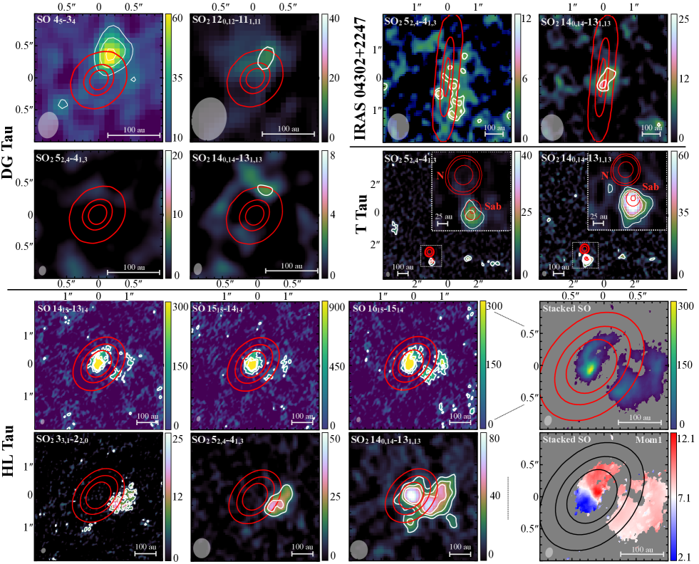
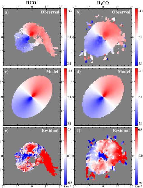
To survey the SO and SO₂ emission in the disks observed by the ALMA-DOT program we inspected the line cubes of the targeted SO and SO₂ lines (see Table 1). For the four disks where emission is detected in at least one of the SO and SO₂ lines, namely DG Tau, HL Tau, IRAS04302, and T Tau, we produce velocity-integrated intensity (moment-0) maps of the lines, integrating over the channels where emission is detected at $>3\sigma$ (the r.m.s. noise per channel of the line cubes is given in Table 2). For the lines showing no emission at the line cube inspection, we integrate over the same velocity range of the detected line(s). Finally, we integrate the moment-0 maps over the disk area (as defined by the area where the 1.3 mm flux is $>5\sigma$) to obtain the disk-integrated line flux summarized in Table 2. Based on the disk-integrated line intensities, three of the ten SO₂ lines probed are detected above 5$\sigma$ confidence in at least one source, one is tentatively detected ($3-5\sigma$), while the remaining six, as well as the ³⁴SO₂ line, are never detected ($<3\sigma$). The four SO₂ lines formally or tentatively detected are the $12_{0,12}-11_{1,11}$ (only surveyed and tentatively detected in DG Tau), the $3_{3,1}-2_{2,0}$ (only surveyed in HL Tau), the $5_{2,4}-4_{1,3}$ (detected in HL Tau, IRAS04302, and T Tau), and the $14_{0,14}-13_{1,13}$ (detected in all sources, although only tentatively in DG Tau and IRAS04302). The SO $4_{5}-3_{4}$ line, which is only probed in DG Tau, as well as the SO $14_{15}-13_{14}$, $15_{15}-14_{14}$, and $16_{15}-15_{14}$ lines, which are only probed in HL Tau, are all firmly detected. Figure 1 shows the moment-0 maps of the detected SO and SO₂ lines compared with the distribution of the disk continuum emission at 1.3 mm.

3.1.1 Spatial distribution of SO and SO₂ emission

Figure 1 shows that the strong SO $4_{5}-3_{4}$ line emission in DG Tau is not located along the direction of its well-known collimated jet, which is detected along $PA_{\rm jet}=225\degree$, i.e., perpendicular to the position angle (PA) of the disk ($PA_{\rm disk}=135\degree$) (e.g., Eislöffel & Mundt, 1998; Podio et al., 2020b). Moreover, the SO emission is not symmetrically distributed across the disk but instead originates from only one side of the disk, the northwest side along the disk major axis. The peak of the emission, detected at 12$\sigma$, is located at 0.4″ (50 au) to the northwest with respect to the continuum peak. The SO₂ $12_{0,12}-11_{1,11}$ line is tentatively detected (3$\sigma$) and peaks at the same position as SO. The SO₂ $14_{0,14}-13_{1,13}$ line is not detected although some marginal flux is visible at the same location after smoothing the image by 1″.

In HL Tau, the SO₂ 5${}_{2,4}-4_{1,3}$, $14_{0,14}-13_{1,13}$, and $3_{3,1}-2_{2,0}$ lines are promptly detected with fluxes up to 13$\sigma$, 17$\sigma$, and 18$\sigma$, respectively. Similarly to what is found for DG Tau, the SO₂ emission is not located along the collimated atomic jet direction ($PA_{\rm jet}=51\degree$, e.g., Mundt et al. 1990), or along the wide-angle outflow cavities probed by CO $1-0$ (ALMA Partnership et al., 2015). The low-excitation SO₂ 5${}_{2,4}-4_{1,3}$ and $3_{3,1}-2_{2,0}$ line emission ($E_{\rm up}\sim 24$ K and $28$ K, respectively) originates from a compact region on the southwest side of the disk. The emission is displaced to the west with respect to the jet direction and is displaced from the center of the continuum emission, extending from a radius of 0.6″ to 1.0″, corresponding to radii of 90 to 150 au. On the other hand, the high-excitation SO₂ $14_{0,14}-13_{1,13}$ line ($E_{\rm up}\sim 93$ K) exhibits both the same displaced component in the SW outer disk and a component from the inner disk, centered on the continuum peak. Similarly to the SO₂ $14_{0,14}-13_{1,13}$ line, the three high-excitation SO lines at $\sim$645 GHz ($E_{\rm up}\sim 253-261$ K) show bright emission in the inner disk and faint emission from the SW outer disk region. The moderate-resolution maps by Wu et al. (2018) resolved SO $5_{6}-4_{5}$ emission to the SW of HL Tau, in line with the SO₂ 5${}_{2,4}-4_{1,3}$ line emission. Our maps show that the central emission detected only in the high-excitation SO and SO₂ lines protrudes toward the north and seems to reconnect, although discontinuously, with the line emission in the SW outer disk region. Given their similar E_up, the three SO lines could be stacked to obtain the maps shown in the last column of the bottom part of Fig. 1. The high spectral and spatial resolution of these data also enables a meaningful intensity-weighted mean velocity (moment-1) map. This map shows that, while the outer component is detected at a constant redshifted velocity, the inner component shows a velocity gradient that is coherent with the disk rotation pattern (see Sect. 3.2.2).

Only weak SO₂ emission is visible from IRAS04302 (Fig. 1). The SO₂ 5${}_{2,4}-4_{1,3}$ line is tentatively detected with 3.5$\sigma$ confidence in the outer disk toward the SW of the star and peaks at a separation of 1.2″ (190 au). The SO₂ $14_{0,14}-13_{1,13}$ line is formally detected (peaking at 5.5$\sigma$) but is only seen close to the continuum center (i.e. in the inner disk).

Table 3: Beam-averaged column density of SO and SO₂ and gas temperature.

Species	Location	$N_{\rm X}$	$T_{\rm rot}$
		(cm-2)	(K)
SO	DG Tau outer disk	$(1.6-6.3)\cdot 10^{14}$	$40-300$a
SO2	DG Tau outer disk	$(0.5-2.3)\cdot 10^{14}$	$40-300$a
SO	HL Tau inner disk	$>2\cdot 10^{15}$	$>350$b
SO2	HL Tau inner disk	$>2\cdot 10^{15}$	$>350$c
SO	HL Tau outer disk	$(0.2-2)\cdot 10^{16}$	$58\pm 19$b
SO2	HL Tau outer disk	$(7\pm 3)\cdot 10^{14}$	$58\pm 19$
SO2	IRAS04302 inner disk	$>10^{14}$	$>75$c
SO2	T Tau S	$(0.3-3.7)\cdot 10^{15}$	$40-300$a
SO2	T Tau knot	$(3\pm 2)\cdot 10^{14}$	42$\pm$20

Finally, significant emission is detected from both the SO₂ 5${}_{2,4}-4_{1,3}$ and $14_{0,14}-13_{1,13}$ lines in proximity to the binary T Tau S (with a flux peak of 8$\sigma$ and 22$\sigma$, respectively). The emission from both lines is displaced from the continuum peak toward the south. Five to six times fainter line emission in the SO₂ 5${}_{2,4}-4_{1,3}$ and $14_{0,14}-13_{1,13}$ lines is also detected in a series of knots located west of T Tau S at a distance of $2.5-5\arcsec$, i.e., $\sim 360-720$ au. No SO₂ emission is detected towards T Tau N.

3.1.2 Column densities and excitation temperatures

To estimate the molecular column density and gas temperature in the SO₂- and SO-emitting regions, we integrate the line emission on a beam area centered on the peak of the SO₂ $14_{0,14}-13_{1,13}$ line which is detected in all the sources studied here. For HL Tau and IRAS04302, the SO₂ emission has two peaks, one in the outer disk and one in the inner disk, and so two integration areas are considered. The same is done for T Tau, where the emission is integrated on the disk of T Tau S and on the closer knot. The beam-integrated line fluxes are summarized in Table 2. For the sources where two or three lines of the same species are detected, the beam-averaged SO and SO₂ column density, $N$, and rotational temperature, $T_{\rm rot}$, can be derived from the beam-integrated line fluxes by performing a standard rotational diagram (RD) assuming local thermodynamic equilibrium (LTE), and optically thin lines. The assumption of LTE is well justified as the gas density in the disk molecular layer ($10^{8}-10^{12}$ cm^-3; e.g., Walsh et al. 2014) is above the critical density of the detected SO₂ lines ($\sim 10^{6}$ cm^-3 for kinetic temperatures of $50-350$ K) and SO lines ($\sim 6\times 10^{5}$ cm^-3 for the $4_{5}-3_{4}$ line detected in Band 5 for DG Tau, and $\sim 1.5\times 10^{7}$ cm^-3 for the high $E_{\rm up}$ lines detected in Band 9 for HL Tau, for kinetic temperatures of $50-350$ K). The line optical depth cannot be estimated as the emission from the ³⁴SO₂ isotopolog is undetected and only up to three lines of SO₂ and SO per source are detected, impeding a full radiative transfer analysis. The column densities estimated here assuming optically thin emission have to be considered as lower limits in the case where the lines are optically thick. For the sources where only one SO₂ line is detected (the SO₂ $14_{0,14}-13_{1,13}$ line, which has large line strength; see Table 1), we use the upper limit on the SO₂ $5_{2,4}-4_{1,3}$ (which is the line with the second highest line strength in Band 6) to perform a RD analysis and retrieve a lower limit on $T_{\rm rot}$ and $N$. The upper limit retrieved for the other undetected SO₂ lines in Band 6, which have lower line strengths, is less constraining and is not used in the linear fit of the RD. However, we check that these upper limits are consistent with the obtained solution as shown in the RD plots in Figure 8. Finally, for DG Tau, where two SO₂ lines are both tentatively detected (at $\sim 3\sigma$), and T Tau S, for which the two detected SO₂ transitions ($14_{0,14}-13_{1,13}$ and $5_{2,4}-4_{1,3}$) peak at different positions, we assumed a range of temperatures ($T=40-300$ K) and, under the assumption of LTE and optically thin emission, we estimate a range of column densities from the brightest detected line. The values of $T_{\rm rot}$ and $N$ obtained for all the sources are reported in Table 3.

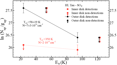
Stringent constraints on the gas temperature and molecular column density are obtained for HL Tau, where the two transitions in Band 6 with the largest line strengths, namely the SO₂ 5${}_{2,4}-4_{1,3}$ and $14_{0,14}-13_{1,13}$ lines, are detected with high S/N. The rotational temperature inferred for the central (inner disk) region probed only by the high-excitation SO₂ line ($E_{\rm up}=93$ K) clearly differs from that inferred for the displaced (outer disk) component where also low-excitation SO₂ lines are detected ($E_{\rm up}=24-28$ K) (see Sect. 3.1.1). In the inner disk, we find a lower limit of 350 K (where the limit is dictated by the nondetection of the 5${}_{2,4}-4_{1,3}$ line in the central region) while in the outer disk we constrain $T_{\rm rot}=58\pm 19$ K. The estimated SO₂ column density is $(7\pm 3)\cdot 10^{14}$ cm^-2 in the outer disk and a factor of two larger in the inner disk. On the other hand, the estimate of the gas temperature from the SO lines is challenged by the narrow range of $E_{\rm up}$ of the three detected lines (253$-$262 K, see Table 1). As the SO emission is co-spatial with the SO₂ emission both in the outer and inner disk, we assume that the gas temperature of the SO-emitting region is the same as for SO₂ (i.e., $58\pm 19$ K in the outer disk and $>350$ K in the inner disk) and estimate the SO column density. We find $N_{\rm SO}=(0.2-2)\cdot 10^{16}$ cm^-2 and $N_{\rm SO}>2\cdot 10^{15}$ cm^-2 for the outer and inner disk region, respectively.

As for DG Tau, the $T_{\rm rot}$ of the emitting region cannot be constrained from SO or SO₂ because of the availability of one SO line and of the faintness of all SO₂ lines. Therefore, we assumed a range of temperatures ($T=40-300$ K) deriving $N_{\rm SO_{2}}=(0.5-2.3)\cdot 10^{14}$ cm^-2, and $N_{\rm SO}=(1.6-6.3)\cdot 10^{14}$ cm^-2.

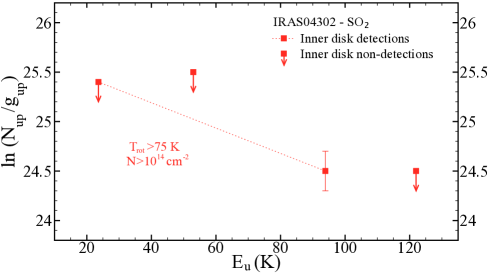
In IRAS04302, we examined the emission from the inner disk region, where the peak of the brightest SO₂ $14_{0,14}-13_{1,13}$ is found. The nondetection of the SO₂ 5${}_{2,4}-4_{1,3}$ emission towards this region leads to a lower limit on $T_{\rm rot}$ and $N_{\rm SO_{2}}$ (75 K and 10¹⁴ cm^-2, respectively).

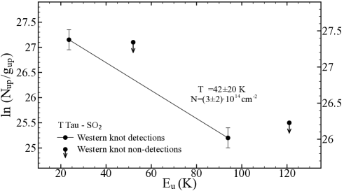
Also, given the large uncertainty affecting the SO₂ 5${}_{2,4}-4_{1,3}$ emission toward T Tau S when integrating over the area centered on the brightest SO₂ $14_{0,14}-13_{1,13}$ line (see the beam-integrated fluxes reported in Table 2) we assumed a range of temperatures ($T=40-300$ K), as done for DG Tau, and estimate the column density for this temperature range: $N_{\rm SO_{2}}=(0.3-3.7)\cdot 10^{15}$ cm^-2. On the other hand, two SO₂ lines were detected toward the brightest knot located at $2.5\arcsec$ on the west of T Tau S, and we were able to constrain $T_{\rm rot}$ as 42 K, yielding $N_{\rm SO_{2}}=(3\pm 2)\cdot 10^{14}$ cm^-2.

3.2 Circumstellar medium from CO, CS, and HCO⁺ lines

In this section, we examine the ambient medium around the disk of each source and relate it to the SO and SO₂ emission studied in Sect. 3.1.

Figure 2: Imagery of DG Tau. (a): moment-0 map of the ¹²CO 2$-$1 line. (b): moment-1 map of the ¹²CO 2$-$1 line. (c): moment-0 of the CS 5$-$4 line. (d): moment-1 of the CS 5$-$4 line. (e): Integrated spectra of CO and CS from the region labelled I in (c). (f): Integrated spectra of CO, SO, and CS from the region labelled II in (c). In each map, red and white (or black) contours indicate the continuum and SO $4_{5}-3_{4}$ line emission, respectively, as in Fig. 1. North is up, east is left.

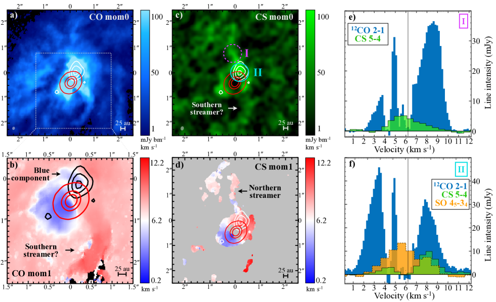
3.2.1 DG Tau

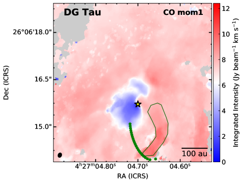
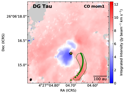
The ¹²CO map of DG Tau (see Fig. 2a) reveals the presence of extended structures on a complex kinematics around the disk. A very bright blueshifted component is present on the redshifted (NW) side of the disk. This component is even brighter than the disk itself (twice as bright as the CO emission on the other side of the disk at the same separation), yielding a blue region in the moment-1 map (Fig. 2b). Interestingly, this blue CO component is spatially coincident with the SO flux described in Sect. 3.1. Another peculiar structure of the CO map is a redshifted structure resembling a streamer to the South. Both the blue component and the putative southern streamer were detected by Güdel et al. (2018) who explained them with an outflow driven by magnetic fields or a stellar wind.

The CS and H₂CO emission from the disk of DG Tau originates from a narrow disk ring (see Podio et al., 2019, 2020b). The emission from both molecules is maximized on the NW side of the disk, which is the region where we detect the CO blue component and SO emission. In Fig. 2c, we show a smoothed version of the CS moment-0 map by Podio et al. (2020b). Two tenuous streamers are visible from both this map (northern and southern streamers in Fig. 2c and d, see also Podio et al., 2020b) and the moment-1 map (Fig. 2d) obtained after clipping fluxes below 5$\sigma$. The faint southern streamer is spatially coincident with the CO counterpart.

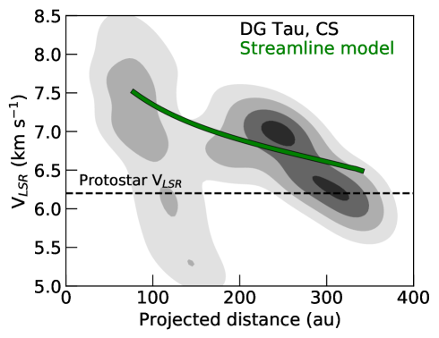
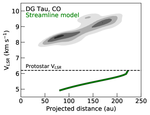
The CS data was analyzed by applying an analytic streamline solution of a rotating sphere collapsing towards a central mass (Mendoza et al., 2009; Pineda et al., 2020) to search for signs of infall (see Appendix B for a description of the modeling process and Appendix B.1 for the modeling results of the DG Tau streamers). The results indicate that the northern streamer is indeed infalling and impacting the disk where the SO emission appears, but the analytic streamline model did not well-describe the southern red-shifted arc-shaped streamer. This may be because the southern streamer is actually an extension of the northern streamer piercing through the disk and in the process of turning back towards the central mass.

Figure 2e shows the spectra of CO and CS integrated on the brightest part of the northern streamer (region I in Fig. 2c). The CS emission is detected over a relatively large velocity range around the systemic velocity ($V_{\rm sys}=6.2$ km s ^-1, Garufi et al. 2021) but peaks at slightly blueshifted velocities ($\sim$5.5 km s^-1). From the comparison with CO, it is clear that the northern streamer cannot be promptly detected in CO because of the absorption by the large-scale cloud from 5.2 to 6.6 km s^-1 (as well as from 3.8 to 4.6 km s^-1). Finally, Fig. 2f reveals that the SO spectrum integrated on the NW outer disk component (region II in Fig. 2c) is spectrally broad ($\sim$7 km s^-1) and peaks at a slightly blueshifted velocity of 5.5 km s^-1, and is therefore closer in kinematics to the northern streamer seen in CS and the CO blue component than to the local redshifted disk (at $\sim$8.5 km s^-1 from the CS).

Figure 3: Imagery of HL Tau. (a) Moment 0 of the HCO⁺ 3$-$2 line (Yen et al., 2019). a_zoom): zoom onto the central region of (a). (b) Moment 1 of the HCO⁺ 3$-$2 line. (c) Moment 0 of the CS 5$-$4 line. (d) Moment 1 of the CS 5$-$4 line. (e) Integrated spectra of HCO⁺, SO₂ $14_{0,14}-13_{1,13}$, and SO $15_{15}-14_{14}$ from the region labelled I in (d). (f) Integrated spectra of HCO⁺, SO₂ $14_{0,14}-13_{1,13}$ and $5_{2,4}-4_{1,3}$ from the region labeled II in (b). In each map, red and white (or black) contours indicate the continuum and SO₂ $14_{0,14}-13_{1,13}$ line emission as in Fig. 1, except contours from (a_zoom) that indicate the SO $15_{15}-14_{14}$ line emission. The arrow points to the inner part of the HCO⁺ streamer visible as a SO protrusion. North is up, east is left.

3.2.2 HL Tau

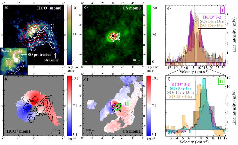
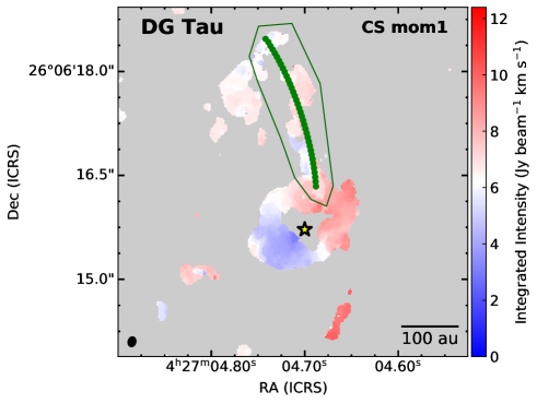
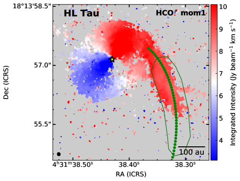
The CO emission from HL Tau is dominated by the prominent outflow cones (see ALMA Partnership et al., 2015). Here, we make use of the HCO⁺ 3$-$2 maps described by Yen et al. (2019) and shown in Fig. 3a and 3b. The comparison with the SO and SO₂ detection described in Sect. 3.1 highlights that the inflowing spiral described by Yen et al. (2019) and designated as a streamer in our figures reconnects with the disk at the position where the outer component of the SO and SO₂ is detected. The SO₂ map even shows a weak protrusion that is spatially coincident with the HCO⁺ streamer. A zoom onto the inner disk region (see Fig. 3a_zoom) highlights the spatial consistency of the HCO⁺ and SO $15_{15}-14_{14}$ line emission. More precisely, the inner part of the HCO⁺ streamer corresponds to the northern protrusion of the central SO component shown in Fig. 1.

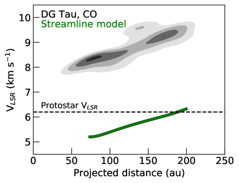
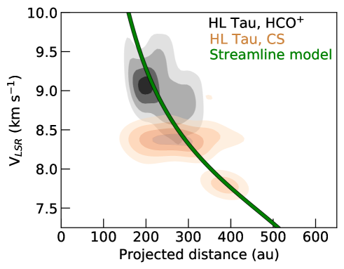
On a larger scale, relatively bright, diffuse CS emission is detected to the west of the star (Fig. 3c). Even though there is no morphologically defined structure like the HCO⁺ streamer, the velocity-weighted map clipped at 5$\sigma$ (Fig. 3d) indicates that the CS to the SW has a peculiar, redshifted velocity comparable to that of the HCO⁺ streamer. When we apply an analytic streamline model to the HCO⁺ and CS data together, we indeed find that both are consistent with an infalling streamer landing where the SO emission extends to the west (see Appendix B.2).

The integrated spectra of the SO and SO₂ lines reveal that the emission from the intersection of disk and streamer (region II in 3d) has the same velocity pattern of the local disk traced by the HCO⁺ emission (Fig. 3f) while the central component (region I) is very broad ($\sim$35 km s^-1, thus matching the tail of HCO⁺) and approximately peaks at systemic velocity ($V_{\rm sys}=+7.1$ km s^-1, Garufi et al. 2021) (Fig. 3e).

Figure 4: Imagery of IRAS 04302+2247. (a) Moment 0 of the ¹²CO 2$-$1 line. b) Moment 1 of the ¹²CO 2$-$1 line. (c) Same as (a) on smaller scale. (d) Same as (b) on smaller scale. (e) Integrated spectra of CO and SO₂ 5${}_{2,4}-4_{1,3}$ from the region labeled I in (d). (f) Integrated spectra of CO from the region labeled II in (d). In each map, red and black contours indicate the continuum and line emission as in Fig. 1. North is up, east is left.

3.2.3 IRAS 04302+2247

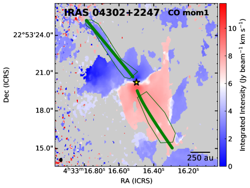
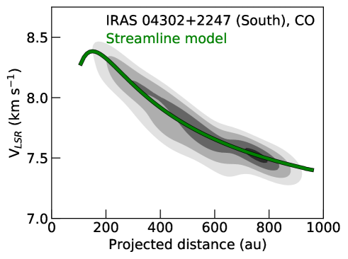
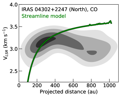
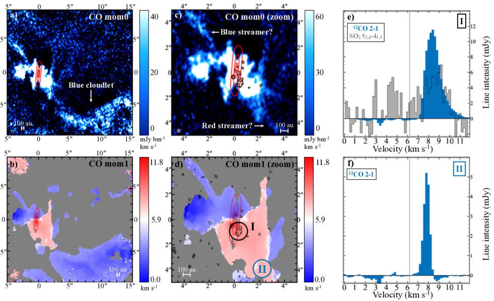
The ¹²CO $2-1$ map of IRAS04302 reveals a complex environment with the presence of several arms. Any result on the global structure is biased by the absence of detectable signal from 3 to 7 km s^-1, that is, for velocities close to the systemic velocity ($V_{\rm sys}=+5.6$ km s^-1, Podio et al. 2020a), because of the absorption by line-of-sight material. A very extended blueshifted cloudlet is seen at large scale to the SW of the source (see Figs. 4a and 4b). Closer to the source, the two most significant structures are the red and blue streamers (Figs. 4c and 4d) that seem to be the mirror opposites of each other. From applying the analytic streamline solutions to these structures (Appendix B.3), we in fact find that the southern, redshifted structure is consistent with a streamer and intersects the disk where the SO₂ signal is detected (see Sect. 3.1), while the northern, blueshifted structure is well described by the streamer model at small radii only. Any connection between the redshifted streamer and the cloudlet remains speculative.

The integrated spectrum of Fig. 4e illustrates that the SO₂ signal is broad in velocity ($\sim 5$ km s^-1) and slightly blueshifted. However, the comparison with CO reveals that it is not at the local disk velocity and that it is closer to that of the red streamer (Fig. 4f) although clearly broader.

3.2.4 T Tau

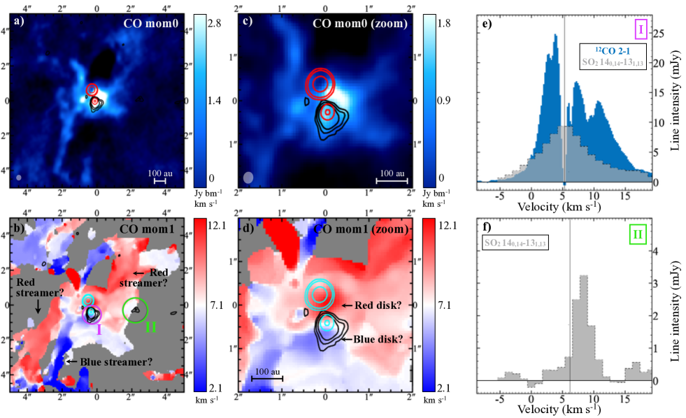
The environment around the T Tau stellar system is notoriously very crowded (see e.g., Duchêne et al., 2005; Kasper et al., 2020). The ALMA-DOT maps of the CS, CN, and H₂CO lines show multiple structures at a large scale (Garufi et al., 2021) that are not in direct relation with T Tau N or S, and we will study these independently. In this work, we only examine the ¹²CO map because the emission peak from this line lies in proximity to T Tau S (see Fig. 5a). In particular, the strongest integrated flux is detected NW of T Tau S, and appears to correspond to a bright bow-shaped feature seen in reflected light (Kasper et al., 2016). The absence of any signal centered on T Tau N could be explained by the nearly face-on geometry of its disk. Generally speaking, such a geometry only yields signal close to the rest-frame velocity and this is barely detectable in our maps because of the absorption by the large-scale material (Garufi et al., 2021).

The moment-1 map highlights the existence of multiple blue and red streamers that approximately run from SE to NW, or vice versa (see Fig. 5b). The streamline analysis of Appendix B does not include these streamers because of the nearly face-on disk geometry of T Tau. On a smaller scale of a few tens of astronomical units (au) (see Fig. 5d), the CO velocity pattern around T Tau S exhibits what is expected from an inclined disk with position angle pointing north, and has a blue disk component to the south and a red disk component to the north. If the observed pattern were genuine disk emission, then the systemic velocity $V_{\rm sys}$ of the T Tau S binary would be around 7$-$8 km s^-1.

The SO₂ signal from T Tau S extracted from region I of Fig. 5b is, similarly to the CO, very broad ($\sim 25$ km s^-1, see Fig. 5e) and centered on $\sim$5 km s^-1. This velocity corresponds to the main CO absorption feature, suggesting that it is the rest frame of the large-scale material. It does however differ from the aforementioned $V_{\rm sys}$ of T Tau S at 7$-$8 km s^-1 constrained by the CO pattern around the source. On the other hand, the signal from the western knot (region II in Fig. 5b) is only detected in a narrow interval around 8$-$9 km s^-1 (see Fig. 5f).

Figure 5: Imagery of T Tau. (a) Moment 0 of the ¹²CO 2$-$1 line. (d) Moment 1 of the ¹²CO 2$-$1 line. (c) Same as (a) on a smaller scale. (d) Same as (b) on a smaller scale. (e) Integrated spectra of CO and SO₂ $14_{0,14}-13_{1,13}$ from the region labeled I in (b). (f) Integrated spectra of SO₂ $14_{0,14}-13_{1,13}$ from the region labeled II in (b). In each panel, red (or cyan) and black contours indicate the continuum and line emission as in Fig. 1. North is up, east is left.

3.3 HL Tau disk model

To determine what impact the streamer might have on the HL Tau disk kinematics, the predicted Keplerian velocity of each pixel is calculated assuming a geometrically flat disk (Pineda et al., 2019). We adopted a stellar mass of 2.1 M_⊙ (Yen et al., 2019), a distance of 147.3 pc (Galli et al., 2018), a systemic velocity $V_{\rm sys}$ of 7.1 km s^-1, a position angle of 135^∘, a disk inclination angle of 35^∘, and a disk outer radius of 250 au (Garufi et al., 2021). We convolved the velocity model with the beam of the HCO⁺ (0.1″$\times$0.09″) and H₂CO ALMA-DOT (0.31″$\times$0.26″) observations. Within the disk radius, we subtracted the Keplerian velocity model, while outside of the disk outer radius we subtracted the systemic $V_{\rm sys}$, ensuring a smooth connection at the boundary between the disk and spiral structure (Akiyama et al., 2019). The disk model and residuals after subtracting the Keplerian model from the HCO⁺ and H₂CO moment-1 maps are shown in Fig. 6. The HCO⁺ and H₂CO velocity patterns after subtracting the expected rotation are very similar. Both reveal redshifted material to the south, north, and in the HCO⁺ streamer region to the west, as well as blueshifted material or material close to the $V_{\rm sys}$ to the east and northwest. These results are discussed in Sect. 4.3.

4 Discussion

The results of Sect. 3 can be summarized as follows:

• The spatial distribution of SO and SO₂ emission detected in the Class I/II disks of DG Tau, HL Tau, IRAS04302, and T Tau does not follow the dust and gas distribution in the disk, that is, it does not probe a symmetric radial and/or vertical disk region as observed in the 1.3 mm continuum or in other molecular tracers such as H₂CO and CS (see, e.g., the overview of the continuum and molecular emission in the ALMA-DOT disks in Figure 1 by Garufi et al. 2021).

• In the cases of DG Tau and HL Tau, the SO and SO₂ emission is not located along the jet direction and/or on the outflow cavities as mapped by previous authors in both atomic (e.g., Mundt et al., 1990; Eislöffel & Mundt, 1998) and molecular (e.g., ALMA Partnership et al., 2015; Güdel et al., 2018) lines.

• In all four disks, we detect SO₂ (as well as SO for DG Tau and HL Tau) emission from only one side of the disk, from a compact region which is displaced by $20$ to $190$ au with respect to the dust continuum peak. This emission is detected at the intersection between the disk and some streamers observed in CO, HCO⁺, or CS.

• The velocities of the SO and SO₂ emission from these outer disk regions are comparable with those of the streamers. Their spectral width is small (5$-$7 km s^-1).

• In the case of HL Tau, IRAS04302, and T Tau, we also detect bright emission centered on the continuum peak from the inner $20$ au disk region. This emission is detected only in the high-excitation SO₂ line ($E_{\rm up}=93$ K) and SO lines ($E_{\rm up}=253-261$ K, only for HL Tau).

• The SO and SO₂ emission from the inner disk is centered at the systemic velocity of the source, and covers a large velocity interval (25$-$35 km s^-1). In the case of HL Tau, the moment-1 map shows that the SO gas has a velocity pattern in agreement with the disk Keplerian rotation pattern observed in other gas tracers.

• The gas temperature associated with the SO and SO₂ emission from the outer disk of HL Tau is $\sim 60$ K, while it is $>75$ K in the inner region of IRAS04302 and $>350$ K in the inner disk of HL Tau.

In this section, we discuss these results, focusing on the origin of the observed SO and SO₂ emission in the context of the observed connection between disk and environment.

Figure 6: HL Tau disk velocity structure analysis. A Keplerian disk model (c and d) is subtracted from the observed HCO⁺ and H₂CO moment-1 maps (a and b, from Yen et al., 2019; Garufi et al., 2021), yielding the velocity residuals of (e) and (f). For both HCO⁺ and H₂CO, outside of the disk radius the $v_{\rm sys}$ is subtracted.

4.1 Inflow or outflow

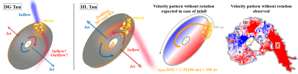
To investigate the origin of the observed SO and SO₂ emission, we must first determine whether the observed structures around the disk are inflowing or outflowing. The northern streamer observed in CS at large scale around DG Tau (see Fig. 2) is most likely the same structure yielding the CO blue component. Güdel et al. (2018) concluded that this component is outflowing material. However, the detection of the CS northern streamer suggests that we are observing an inflowing structure, which is confirmed by the analytic infalling streamline model in Appendix B.1. This is appreciable from the sketch of Fig. 7. On the other hand, the southern streamer (see Fig. 2) could be either inflowing or outflowing, because it may be associated with the northern streamer piercing through the disk and about to turn back towards the young stellar object. In both cases, the angle of incidence with the disk should be smaller than the disk inclination (35°, Podio et al., 2020b) to enable a receding velocity. It is therefore tempting to propose that the southern streamer is the continuation of the northern streamer. In that putative case, a significant amount of material should not efficiently accrete onto the disk but should instead deflect by a considerable angle driven by the disk rotation. In other words, redshifted disk material would cause blueshifted accreting material to become redshifted outflowing material.

Figure 7: Illustrative sketch of the environment of DG Tau and HL Tau. The third panel shows the velocity pattern expected in case of uniform infall after rotation subtraction. The fourth panel shows the observed HCO⁺ velocity pattern after rotation subtraction (see Fig. 6).

.

The interpretation of the streamer in HL Tau (see Fig. 3) is rather intuitive. Inflowing material is impacting the disk on the redshifted side with a coherent direction (NE, see the sketch of Fig. 7). This is the same conclusion as that drawn by Yen et al. (2019), and is supported by our streamline modeling in Appendix B.2. The kinematics of the material around HL Tau is further discussed in Sect. 4.3.

Confirming the inflow of material in the red and blue streamers of IRAS04302 (see Fig. 4) is more complicated, because these streamers lie along the outflow cavity. This source is also known as the butterfly star because of its prominent bipolar morphology observed by Lucas & Roche (1997) and Padgett et al. (1999), which is recurrently interpreted as outflow cavities. These structures are probably not evident in our CO maps because their expanding projected velocity is nearly zero given the disk edge-on geometry, and any material at the source systemic velocity is not observable (see Sect. 3.2.3). In principle, the intrinsic outflow rotation may add a velocity component that enables some material to emit at detectable velocities. However, in DG Tau B and HL Tau (Garufi et al., 2021; ALMA Partnership et al., 2015), the outflow rotation only introduces a $\pm 1$ km s^-1 contribution to the net projected velocity and therefore does not change this view. Geometrically, the blue and red streamers of IRAS04302 could be instead part of the outflow cavities but this would require a mechanism that induces a large rotation velocity on only one side of the outflow cavities; furthermore, our analytic streamline modeling supports the infall scenario for both streamers (Appendix B.3). Also, the structures in question do not seem to originate from the star (see Fig. 4) and therefore it is more likely that we are observing accreting features similar to the cases of DG Tau and HL Tau.

Finally, the case of T Tau is very complex. The main emission is clearly associated with T Tau S and is extended toward the south (see Fig. 5). The Subaru and ALMA observations by Yang et al. (2018) and Manara et al. (2019) suggest that the circumbinary disk of T Tau S is approximately oriented north$-$south, in agreement with our speculations outlined in Sect. 3.2.4. In this scenario, the rest-frame velocity of the disk would be 7$-$8 km s^-1, and the SO₂ emission peaking at 5 km s^-1 (see Fig. 5e) would be blueshifted, in analogy with the velocity of the disk toward the south. This may suggest that the SO₂ signal is disk emission. Alternatively, it could be associated with one of the several outflows inferred in this system (Herbst et al., 1997, 2007). A blueshifted, wide-angle outflow to the SE is believed to originate from T Tau S (Kasper et al., 2016). It is tempting to associate the prominent CO blueshifted arm from Fig. 5b to this outflow but its origin does not seem to be T Tau S. On the other hand, the series of SO₂ knots visible from Figs. 1 and 5 is likely associated with the east–west outflow from T Tau N (Bohm & Solf, 1994), and in particular the western knots lie in the direction of the prominent bow shock detected in the NIR (Kasper et al., 2020), but at a larger separation.

4.2 Origin of the SO and SO₂ emission

The localized nature of the SO and SO₂ emission at the intersection between disk and molecular streamers around DG Tau and HL Tau indicates a confined increase of column densities. The most likely origin of such a localized increase is shocks due to the infalling streamers impacting the disk, which could cause a release of SO and SO₂ molecules from the sputtered dust grain mantles. In fact, any thermal release of SO and SO₂ in the disk layer at temperatures above their evaporation temperature would instead result in an azimuthally symmetric distribution of emission. These shocks would be reminiscent of those associated with Class 0 sources with a denser protostellar envelope. In these earlier objects, such as L1527 or B335 (e.g., Sakai et al., 2014, 2017; Oya et al., 2016, 2017; Imai et al., 2019), slow shocks (around 1 km s^-1) occur at the transition zone of the infalling and rotating envelope with the protostellar accretion disk, causing an enhancement of the SO emission in a ring-like structure. In the ALMA-DOT sample studied in this work, the envelope is largely dissipated. Therefore, a “well-behaved” symmetric ring of shocked material in front of the centrifugal barrier is not expected. Instead, shocks are located along the late infalling streamers still feeding the young stellar objects. The temperatures derived in the SO- and SO₂-emitting region ($\geq$ 60 K, see Sect. 3.1.2) are in agreement with emission from shocked material.

As discussed in Sect. 3.1.1, HL Tau also shows a bright SO and SO₂ component centered on the star. The emission from these regions may also be related to the action of inner jets and outflow (e.g., Podio et al., 2021) or to the innermost regions of disk and envelope (e.g., Harsono et al., 2021) where dust mantles can sublimate, thus resembling a hot-corino chemistry. Booth et al. (2021) also showed an asymmetric SO and SO₂ emission co-spatial with a dust crescent where the molecular enhancement would be related to the sublimation of ices at the edge of a dust cavity at a separation of $\sim$ 50 au. However, in the case of HL Tau presented here, a further explanation is possible. The central SO component in question is clearly protruded toward the shocked region at $\sim$100 au from the star following the inward motion of the HCO⁺ streamer (see Figs. 1 and 3). This suggests that the SO and SO₂ molecules released in the shock at $\sim$100 au spiral toward the star before any chemical reprocessing occurs. The drifting timescale can be coarsely estimated from the morphology of the SO spiral, covering approximately 180$\degree$ (see the sketch in Fig. 7). The orbital period at 100 au from a 2.1 $\rm M_{\odot}$ star (Yen et al., 2019) is $\sim$700 yr. Thus, the spiraling material drifts from 100 au to the star in less than 350 yr, corresponding to a velocity of 1$-$2 km s^-1. These velocities are those of the SO and SO₂ emission at the shock location and of the HCO⁺ accreting streamer (see Fig. 3f), giving support to the proposed explanation. A timescale of a few hundred years is also shorter than the expected timescale needed for the SO and SO₂ abundances to significantly decrease after the occurrence of a shock. This value depends on a number of parameters, but, following for example Pineau des Forets et al. (1993), Charnley (1997), and Taquet et al. (2019), can be roughly estimated as more than 10³ yr, before their abundances are decreased by one order of magnitude.

4.3 Influence of the streamer on disk kinematics in HL Tau

The dust rings of HL Tau lie in the geometrically thin disk midplane (ALMA Partnership et al., 2015) and do not show signs of disturbance in the regions of the disk that spatially overlap with the streamer. This indicates that the streamer spirals into the central region without passing through the disk midplane while the gas kinematics in the molecular layer are clearly affected by the accreting material (Sect. 3.2.2). This finding is consistent with models of disk accretion occurring at the upper layer of the disk surface (Bai et al., 2016; Riols et al., 2020), and is among the first direct detections of surface accretion at large radii ($50-100$ au), while recent evidence was provided for the inner regions of the disk ($<10$ au, Najita et al., 2021).

To interpret the observed velocity pattern of HCO⁺ and H₂CO after removing the expected Keplerian rotation (see Fig. 6), we must first consider that a uniform infalling or inwardly drifting component should be reflected in the residual maps. For the geometry of the disk of HL Tau (with the far side of the disk to the NE; see sketch of Fig. 7), a blueshifted infalling component should appear to the NE and a redshifted infalling component to the SW. The SE portion of the disk (region 0 in Fig. 7), which does not significantly overlap with the accreting material, shows this behavior.

Conversely, the NW portion of the disk shows the expected redshifted component associated with the streamer (region I), as well as a blueshifted component near the intersection with the disk (region II) and a red component where the SO and SO₂ molecules are thought to drift inward (region III). A possible interpretation of the blueshifted material in region II is that the accreting material heats the local disk, resulting in a puffed-up uppermost disk layer that is probed in our maps by its approaching velocity. After that, the cooling streamer material moves closer to the disk midplane and pushes the denser disk material as it orbits, adding a receding velocity component to the net velocity pattern in region III. After this point, the streamer material has drifted inwards to the central protostar (Sect. 4.2) without ever crossing the disk midplane, leaving the SE portion of the disk (region 0) undisturbed from the expected rotation and uniform infall pattern. This proposed scenario could be tested with modeling.

5 Conclusions

Increasing attention from the planet-formation community is being placed on the interaction between planet-forming disks and their surrounding medium. The discovery of several streamers feeding the disk (e.g., Akiyama et al., 2019; Yen et al., 2019; Pineda et al., 2020) offers the opportunity to study how disk accretion proceeds at late stages, when planet formation is possibly already ongoing.

In this study, we show some extended structures resembling the aforementioned streamers around four sources that are still partly embedded in their natal cloud (Class I or early Class II objects). More importantly, we revealed SO and SO₂ emission that appears to correspond to the intersection between disk and streamers. Two of the four cases in question, DG Tau and HL Tau, are clear cases of inflowing material impacting the circumstellar disk and inducing a shock that is traced by emission of SO and SO₂ discretely localized on the region where the streamers connect to the disk. Unlike younger Class 0 sources, such shocks are confined to specific disk regions (e.g., Lee et al., 2019).

While in DG Tau the SO and SO₂ emission is only detected at 50 au from the star, in HL Tau their emission is probed from the outermost disk region, where the shock occurs, down to the innermost disk region. Our interpretation of the inner component of the emission is that the SO and SO₂ molecules released in the shock in the outskirts of the disk spiral toward the star in less than 350 years before any chemical process may occur. We also reveal that the disk kinematics is altered by the accreting material, as the disk shows a blueshifted component in proximity to the shock that can be ascribed to heated material being uplifted toward the observer.

In IRAS 04302+2247, the SO₂ emission is much weaker but is also possibly associated with the physical intersection between the disk and the streamer. Finally, T Tau is more ambiguous because of the complex environment. It is still possible that the SO₂ emission detected in this target originates from inflowing material, although the presence of prominent outflowing structures offers a valid alternative mechanism that could induce the observed shocks.

The possibility that Class I and II planet-forming disks in Taurus or other relatively old star-forming regions are characterized by accreting streamers infalling onto the disk and shocking its material is a realistic possibility that must be taken into account when analyzing the disk structure. Our observations demonstrate that the circumstellar clouds and protoplanetary disks have complex, dynamic structures and that material is most likely continuously fed onto the disk, even in Class II sources, changing the disk temperature and density profiles, as well as altering its chemistry. This addition of material onto the protoplanetary disk should be considered when modeling planet formation and calculating planetary mass budgets. In addition, such accretion processes should also be considered in regards to the stability of the protoplanetary disk. The prototypical example described in this work is also the most studied, namely HL Tau, where the presence of a shock that is possibly altering the whole disk kinematics has not been considered before. This paper further shows that S-bearing molecular species such as SO and SO₂ may be used to probe such accretion shocks caused by late accretion events onto the disk in Class I and II objects, thus extending a branch of investigation that has been profitable in younger, Class 0 sources.

Appendix A Rotational diagrams

The rotational diagrams obtained for the SO₂ lines detected in HL Tau (outer and inner disk), IRAS04302, and the knot located $2.5\arcsec$ west of T Tau S, are shown in Figure 8.

Figure 8: Rotational diagrams of the SO₂ lines detected for HL Tau (outer and inner disk), IRAS04302, and the knot located $2.5\arcsec$ west of T Tau S. The derived values of $T_{\rm rot}$ and $N$ are labeled. The upper limits for undetected SO₂ are overplotted to check for consistency with the obtained solution.

.

Appendix B Confirming infall with streamline models

The trajectory of material infalling towards a central mass through a streamer can be described by an analytic streamline model of material in a rotating and collapsing sphere (see Mendoza et al. 2009; Pineda et al. 2020). This analysis constitutes a generalization of the Ulrich profile, which is often used to describe material in systems with both envelopes and disks (Ulrich 1976). When possible, we manually and iteratively search for solutions of the streamline model which describe both the spatial and kinematic structure of the possible streamers. The T Tau data were not suitable for such an analysis because of the nearly face-on disk geometry, which makes it nearly impossible to kinematically discriminate between different models.

Several parameters of the streamline models were fixed for consistency with previous ALMA-DOT studies (Garufi et al. 2021): the central stellar mass ($M_{star}$), the central rest velocity of the system ($V_{lsr}$), the disk inclination angle ($I.A._{disk}$), and the disk position angle ($P.A._{disk}$). Parameters that were manually explored in the streamline modeling process include the initial streamline positional parameters of radius, polar angle, and azimuthal angle on the rotating sphere ($r_{0}$, $\theta_{0}$, $\phi_{0}$). The dynamical parameters of the streamline initial angular velocity ($\Omega_{0}$) and initial infall velocity ($v_{r,0}$) were also explored. The model parameters that we successfully found to largely reproduce the spatial and kinematic structures are presented in Table 4, and a brief discussion of each of the streamers in DG Tau, HL Tau, and IRAS 04302+2247 are discussed in the following sections.

Table 4: Streamline model parameters

Parameter	DG Tau	HL Tau	IRAS 04302+2247 (South)1	IRAS 04302+2247 (North)1
Fixed parameters:
$M_{star}$	0.3 M⊙	2.1 M⊙	2.0 M⊙	2.0 M⊙
$V_{lsr}$	6.2 $\rm km\,s^{-1}$	7.1 $\rm km\,s^{-1}$	5.9 $\rm km\,s^{-1}$	5.9 $\rm km\,s^{-1}$
$I.A._{disk}$2	35∘	47∘	81∘	81∘
$P.A._{disk}$3	135∘	138∘	355∘	355∘
Explored parameters:
$r_{0}$	450 au	700 au	1200 au	1200 au
$\theta_{0}$	100∘	95∘	70∘	120∘
$\phi_{0}$	295∘	240∘	315∘	135∘
$\Omega_{0}$	$2.0\times 10^{-12}$ s-1	$7.0\times 10^{-12}$ s-1	$2.0\times 10^{-12}$ s-1	$5.0\times 10^{-13}$ s-1
$v_{r,0}$	0.4 $\rm km\,s^{-1}$	0.1 $\rm km\,s^{-1}$	2.1 $\rm km\,s^{-1}$	4.3 $\rm km\,s^{-1}$

B.1 DG Tau

DG Tau has a northern streamer traced in CS and well-modeled both spatially and kinematically by an infalling streamline model (see Fig. 9). The infalling streamer lands in the disk where there is SO emission (compare to Fig. 2). The correspondence between the streamer impact zone and the SO emission indicates that the SO is likely tracing an accretion shock of material entering the disk from the envelope through the streamer.

Conversely, the redshifted southern arc is not well described by the streamline model. In Figures 10 and 11, we show our two best attempts to model the redshifted southern arc in CO with different rotational geometries. For both models, we leave the disk orientation the same as it was in the modeling for the northern streamer traced in CS. For Figure B.2, we use a rotational geometry where the envelope co-rotates with the disk, which we have used for the other successful streamline models in this work and which would be expected from a simple scenario where the disk formed within a rotating envelope. The model parameters $M_{star}$, $V_{lsr}$ $I.A._{disk}$, and $P.A._{disk}$ remain the same as reported in Table 4, and $r_{0}$ = 300 au, $\theta_{0}$ = 110^∘, $\phi_{0}$ = 60^∘, $\Omega_{0}$ = $1.0\times 10^{-11}$ s^-1 and $v_{r,0}$ = 0.0 km s^-1. The streamline model curvature is oppositely curved with respect to the structure of the redshifted arc, and the velocities are under-predicted by $\sim$3 km s^-1. For Figure 11, we show a model where the envelope counter-rotates with respect to the disk, which could be the case if the redshifted southern arc were an infalling captured cloudlet. Here, $I.A._{disk}$ and $P.A._{disk}$ have rotations applied to maintain the same physical orientation of the disk while changing the rotation direction of the infalling streamers to counter-rotate with respect to the disk. $r_{0}$ = 300 au, $\theta_{0}$ = 80^∘, $\phi_{0}$ = 110^∘, $\Omega_{0}$ = $6.0\times 10^{-12}$ s^-1 and $v_{r,0}$ = 0.0 km s^-1. In this case, while the spatial curvature of the arc is well matched, the velocities remain under-predicted by $\sim$3 km s^-1.

Considering that the redshifted southern arc seems to have a coherent velocity structure with the northern streamer, this may indicate that material from the northern streamer may have enough momentum to pass through the disk midplane and is beginning to curve back towards the young stellar object in the redshifted arc. Hence, the redshfited arc may be a putative southern extension of the northern streamer. The analytic streamline model would be unable to model such a complex scenario where material passes through the midplane, because the model assumes that any material reaching the midplane will be met by material in a mirror-opposite streamline from the opposing hemisphere and cannot therefore vertically pass through the disk (Mendoza et al. 2009). The redshifted arc could also be a cloudlet in the process of being captured that is moving with a trajectory not well described by the analytic streamline model or potentially disturbed by the outflow.

Figure 9: Infalling streamline model for the DG Tau streamer. Top: Streamline model, plotted in green, on top of the moment-1 map of CS, spatially matching the observed streamer emission to the north (outlined in the green polygon). Bottom: Velocity components of CS taken from inside the green polygon plotted as a function of projected distance from the central young stellar object, with varying levels of kernel density estimation of the velocity plotted as filled contours. The contours start at 0.5$\sigma$ and progress in steps of 0.5$\sigma$, where $\sigma$ is from a bivariate normal distribution (see also Pineda et al. 2020). The streamline model, shown in green, describes most of the kinematics of the system in addition to the spatial match shown in the top panel. The main deviation is a small amount of blue-shifted emission in the streamer at a projected distance of $\sim$100-150 au from the central young stellar object.

Figure 10: Infalling streamline model for the red-shifted southern arc structure (outlined in the green polygon), with the same disk orientation and rotation geometry used for the northern streamer model (Fig. 9). Top: Streamline model, plotted in green, on top of the moment-1 map of CO, showing the model curvature with this rotation geometry is opposite to the spatial structure of the southern redshifted arc. Bottom: Velocity components of CO taken from inside the green polygon plotted as a function of projected distance from the central young stellar object, with varying levels of kernel density estimation of the velocity plotted as filled contours and contours calculated as in Fig. 9. The streamline model consistently under-predicts the velocity of the arc structure by $\sim$3 km s^-1.

Figure 11: Infalling streamline model for the redshifted southern arc structure (outlined in the green polygon), with the same disk orientation but opposite rotation geometry used for Fig. 10. Top: Streamline model, plotted in green, on top of the moment-1 map of CO, showing the model curvature well matches spatial structure of the southern redshifted arc with the envelope rotation counter-rotating with respect to the disk. Bottom: Velocity components of CO taken from inside the green polygon plotted as a function of projected distance from the central young stellar object, with varying levels of kernel density estimation of the velocity plotted as filled contours and contours calculated as in Fig. 9. Here, the streamline model also consistently under-predicts the velocity of the arc structure by $\sim$3 km s^-1, even though the spatial structure is well matched by the model.

B.2 HL Tau

The streamer of HL Tau to the southwest of the disk is traced by HCO⁺ near the disk, with radii further from the disk traced by CS. Both the HCO⁺ and CS in the streamer are well described by the analytic infalling streamline model (see Fig. 12). This is the first time a single streamer has been traced and modeled with different molecular tracers at different projected distances from the system center. The streamer lands where the SO extends to the west as seen in Fig. 3, tracing the shocked impact zone of the streamer.

Figure 12: Infalling streamline model for the HL Tau streamer. Top: Streamline model, plotted in green, on top of the moment-1 map of HCO⁺, spatially matching the observed streamer emission extending to the south (outlined in the green polygon). The model predicts that the streamer should extend beyond the HCO⁺ emission, into a region traced by CS (see Fig. 3). Bottom: Velocity components of HCO⁺ (black) and CS (orange) taken from inside the green polygon plotted as a function of projected distance from the central young stellar object, with varying levels of kernel density estimation of the velocity plotted as filled contours and contours calculated as in Fig. 9. The streamline model is shown in green, and highlights that both HCO⁺ and CS trace different parts of the same infalling streamer.

B.3 IRAS 04302+2247

IRAS 04302 has two infalling streamers that can be identified by the analytic streamline modeling of the CO emission (Fig. 13). The redshifted southern streamer seems to feed from the blueshifted captured cloudlet, with SO present in the disk where the model predicts the impact zone of the streamer to be (compare Fig. 13 and Fig. 4). The blueshifted northern streamer is well described by the streamline model at small radii, though at larger radii the model over-predicts the velocity of the observed material, and suggests that the larger scale environment around the disk is likely much more complicated than the simple streamline model can account for.

Figure 13: Infalling streamline model for the two IRAS04302 streamers. Top: Streamline models, plotted in green, on top of the moment-1 map of CO, spatially matching the observed streamer emission to both the south and north (outlined in the green polygons). Middle and bottom: Velocity components of CO taken from inside the south and north green polygons, respectively, plotted as a function of projected distance from the central young stellar object, with varying levels of kernel density estimation of the velocity plotted as filled contours and contours calculated as in Fig. 9. The streamline models are shown in green. For the southern streamer, the CO emission is entirely described by the streamline model. For the northern streamer, the streamline model corresponds well with the emission at radii less than 400 au, but the model over-predicts the velocity at larger radii, hinting at a more complex velocity field in this system.