Non-linear Boson Sampling
Abstract
Boson Sampling is a task that is conjectured to be computationally hard for a classical computer, but which can be efficiently solved by linear-optical interferometers with Fock state inputs. Significant advances have been reported in the last few years, with demonstrations of small- and medium-scale devices, as well as implementations of variants such as Gaussian Boson Sampling. Besides the relevance of this class of computational models in the quest for unambiguous experimental demonstrations of quantum advantage, recent results have also proposed first applications for hybrid quantum computing. Here, we introduce the adoption of non-linear photon-photon interactions in the Boson Sampling framework, and analyze the enhancement in complexity via an explicit linear-optical simulation scheme. By extending the computational expressivity of Boson Sampling, the introduction of non-linearities promises to disclose novel functionalities for this class of quantum devices. Hence, our results are expected to lead to new applications of near-term, restricted photonic quantum computers.
Introduction. – Quantum technologies promise to provide speed-up in several fields, ranging from intrinsically secure long-distance quantum communication [1] to a novel generation of high-precision sensors [2], and enhanced computational and simulation capabilities [3]. Among the currently developed experimental platforms, in the last few years photonic technologies have recently experienced a technological boost in all fundamental components, namely photon sources, manipulation and detection [4].
Recent studies have focused on identifying suitable dedicated classically-hard tasks, with the aim of leveraging the necessary technological resources and system size to reach the quantum advantage regime [5, 6]. Such regime corresponds to the scenario where a quantum device solves a given task faster than any classical counterpart. Within this context, a computational problem named Boson Sampling [7] has been defined as a promising approach. This problem, that consists in sampling from the output distribution of a system of non-interacting bosons undergoing linear evolution, is a classically-hard task (in ) while it can be naturally solved by a linear optical photonic system. Such sampling problem has also subsequently inspired other classes of sampling problems [8, 9] suitable to be solved with different quantum hardware [10, 11, 5].
Starting from the original proposal [7], several experimental implementations of Boson Sampling instances [12, 13, 14, 15, 16, 17, 18, 19, 20, 21, 22, 23] and of recently proposed variants [24, 25, 26, 27, 28] have been reported [29]. In particular, hybrid algorithms based on Gaussian Boson Sampling have been proposed for various tasks: quantum simulation [30, 31, 32, 27, 33], optimization problems [34], point processes [35] graph theory [36, 37, 38], and quantum optical neural networks [39]. Very recently, impressive experimental implementations of Gaussian Boson sampling have been reported [6, 40]. Besides the technological advances reported in the last few years, several studies have also focused on studying and improving classical simulation of Boson Sampling [41, 42, 43, 44, 45, 46], and on defining the limits for simulability in the presence of imperfections, in particular losses and partial photon distinguishability [47, 48, 49, 50, 51, 52, 53, 54]. All these studies aimed at establishing a classical benchmarking framework for Boson Sampling, and currently place the threshold for quantum advantage in such a system to photons in a network composed by optical modes. Recent improvements in photon sources [55, 56, 57, 58, 59, 60] enabled first Boson Sampling experiments with a number of detected photons up to [23]. However, reaching the quantum advantage regime with a photonic platform solving the original formulation of the task [7] still requires a technological leap to enhance single-photon generation rates and indistinguishability, and to reduce losses in the current platforms for linear-optical networks.
In this Letter, we introduce the adoption of non-linear interactions at the few-photon level within the Boson Sampling framework as a route to increase the complexity and reduce the threshold for the quantum advantage regime. This possibility is encouraged by recent advances showing the first experimental demonstrations of non-linear photonic processes within solid state devices [61]. We will first describe the introduction of non-linearities within the otherwise linear evolution. Then, we will provide an upper bound on the complexity of the enhanced devices via a simulation scheme based on auxiliary, linear-optical gadgets. We will discuss both the asymptotic and finite cases, leveraging results from the well-established linear Boson Sampling framework [7].
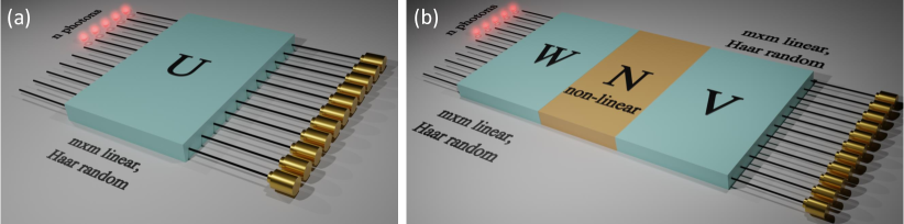
Boson Sampling. – Boson Sampling [7] is a computational task which corresponds to sampling from the output distribution of indistinguishable, non-interacting photons after evolution through a -mode linear network [see Fig. 1(a)].
Given an interferometer described by a unitary matrix , the transition amplitude from input to output state can be written as:
| (1) |
where is the matrix permanent, are the occupation numbers of states , and is the matrix obtained by selecting rows and columns of according to the and respectively. Calculation of permanents of matrices with complex entries is in the #P-hard computational complexity class [62]. In Eq. (1), is the unitary transformation acting on the Hilbert space of photons in modes, that corresponds to the linear evolution on the optical modes. Due to the linearity of the evolution, is an homomorphism [63]. This means that, if a given evolution is the sequence of two linear networks and , the overall evolution can be written in terms of permanents of submatrices of .
In Ref. [7] it was shown that sampling (even approximately) from the output distribution of such a system is classically hard if (i) the input state has at most one photon per mode, (ii) is drawn randomly from the uniform Haar measure, and (iii) the number of modes and photons satisfy .
Non-linear Boson Sampling. – Let us now consider the scheme of Fig. 1(b). An input state of indistinguishable photons undergoes a -mode evolution divided in three steps. While steps 1 and 3 are linear evolutions and drawn from the Haar ensemble, the intermediate step 2 now consists of a non-linear evolution . This transforms a state as , where and is the set of tuples corresponding to photons in modes. In this equation, function represents the transition amplitude determined by the non-linear evolution. We assume has an efficient classical description, e.g., it is given by the composition of a small number of few-mode non-linear transformations, or by a Hamiltonian with a simple form in terms of the field operators.
Let us now write the overall transformation of input state according to the three-step evolution , which includes linear transformations of the form given by Eq. (1), and the non-linear :
| (2) | ||||
This amplitude is written as a Feynman path sum over all possible basis states just before and after the non-linear evolution step. If the permanent distribution was peaked, it might be possible to obtain a good approximation to Eq. (2) by summing over only the dominant terms. Haar random matrices, however, display an anti-concentrated, relatively flat distribution [7]. In [64] we provide numerical evidence for this, showing that to account for of the total probability mass function, we need to calculate the probabilities associated with respective fractions of all possible outcomes; moreover, this behavior is nearly independent of and .
Of course, there may be computational shortcuts to evaluating Eq. (2), other than the explicit sum over paths. For example, if we replace the non-linear term by a linear term, the amplitude can be evaluated as a single permanent. This motivates us to investigate different ways to assess the complexity of non-linear Boson Sampling.
Single-mode non-linear phase shift gate. – Let us proceed by studying a specific example of non-linear evolution consisting of a single non-linear phase gate introduced in mode . The unitary operator describing this gate can be written as . Its action on a generic -mode state leads to a function of the form Inserting this choice of non-linear evolution into the general expression (2) we obtain:
| (3) | ||||
Eq. (3) can be rearranged in the following form (see [64]):
| (4) | ||||
Here, is a unitary transformation composed by the sequence , and , where replaces the non-linear phase in layer with a linear phase shift described by the operator . Equation (4) clearly shows that the departure from linear evolution is due only to bunching terms, corresponding to more than a single photon in mode .
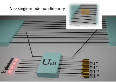
Bounding complexity via linear-optical simulation using auxiliary photons. – An upper bound on the complexity of non-linear Boson Sampling can be obtained by devising a specific linear-optical simulation algorithm, that we discuss below for the case of a single-mode non-linear phase.
The simulation is based on the results by Scheel et al. [65], describing how auxiliary photons and modes can be used, together with linear optics, to induce effective non-linear gates. In particular, given a single mode state in the photon number basis , it is possible to apply a polynomial of degree in the photon number operator to by injecting the state in mode of a suitably chosen -mode linear-optical gadget described by unitary , where the auxiliary modes are injected with a single photon state . The desired output state is obtained upon conditional detection of a single photon on each of the auxiliary modes. If the input state has a maximum number of photons , a polynomial of degree in is sufficient to obtain the general evolution from to with arbitrary coefficients [66]. The success probability of the operation is equal to [65], where is the submatrix of obtained by removing row 1 and column 1 from the full matrix.
Finding the effective linear-optical simulation unitary has been done previously only for a few types of gates and small [67, 65, 68, 69], as the computational effort seems to scale exponentially with . Nevertheless, even limited non-linear gate simulations can be quite versatile, as it is known that almost any non-linear gate can be combined with linear optics to generate arbitrary non-linear gates [70] - for details, see [64].
In Fig. 2 we describe the linear-optical, postselection-based gadget that can be used to simulate single-mode non-linear gates. We see that the -mode linear optical gadget (with ) replaces the single-mode non-linear gate. In the gadget, mode and the single photons undergo the effective unitary . This linear-optical simulation approximates the non-linear Boson Sampling evolution upon detection of photons at the auxiliary output modes.
Using the state-of-the-art weak classical simulation algorithm of Clifford and Clifford [42], we can simulate the enlarged (, ) linear optical system, postselecting only those events where a single photon is measured in each of the auxiliary modes (see [64] for more details). This results in a classical simulation algorithm for the non-linear Boson Sampling experiment.
Let us now discuss some issues that arise when using this scheme to simulate non-linear Boson Sampling in either the asymptotic regime of large numbers of photons/modes, or in the finite setting.
Non-linearities in the asymptotic setting. – Assuming uniformly drawn, Haar-random interferometer unitaries, it has been shown that the appropriate scaling between the original number of modes and number of photons will result in asymptotic suppression of multi-photon collisions. More precisely: if , then -fold collisions are suppressed, when go to infinity [71]. In particular, this will be true for the photon occupation numbers at the non-linear gates. So, by choosing , at most photons will asymptotically be present at each non-linear gate, which means the linear-optical simulation (or classical simulation based on it) can be done with only auxiliary photons per non-linear gate. As we will soon show, such a simulation for small , e.g. can be readily obtained. These simulations using are sufficient for an asymptotically perfect simulation for the usual Boson Sampling regime of . In other words, in this setting there is a precise correspondence between one single-mode non-linear phase gate and two extra auxiliary photons. More generally, the scaling of with dictates how many auxiliary photons are needed for asymptotically perfect simulation of a non-linear phase gate .
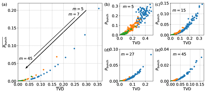
Non-linearities in the finite setting. – The setting with finite is experimentally relevant, and in this case there will be no strict suppression of multi-photon collisions at the non-linear gates. Setting results in an exact classical simulation of non-linear Boson Sampling. When we will have only an approximate simulation. As an example, when numerical results suggest that a number of auxiliary photons equal to should provide a sufficiently accurate simulation given the large effective suppression of bunching at the output of Haar-random unitaries (see [64]).
There are two main features that increase the simulation complexity. First, finding an effective unitary that uses photons for a linear-optical simulation seems to require the computation of permanents of matrices [65, 64], which results in a classical runtime that increases exponentially with . The other cost incurred is the postselection overhead. From all the simulated events on the enlarged linear-optical set-up with photons, we only use events where the auxiliary photons were detected at the linear-optical simulation gadget. This will happen with a probability . There is some evidence that the maximum value of tends to decrease as increases [72].
We have performed numerical simulations of non-linear Boson Sampling with a single non-linear phase in the finite setting, using the classical algorithm based on linear-optical simulation. The results are shown in Fig. 3 for (, ) and (, ). As expected, having results in exact sampling from the non-linear process, and in fact (once the appropriate gadget has been determined) is numerically found to be more computationally effective than directly using Eq. (2). For fixed , note that the simulation error decreases with increasing , since bunching events become rarer. These results suggest that the crucial parameter for the simulation complexity is the scaling between and (see also [64]). The regime when is particularly interesting, as there is a trade-off between a faster classical simulation algorithm [46], and the increased complexity required to find the linear-optical gadget unitary for larger .
If the number of auxiliary photons , the simulation scheme based on linear-optical gadgets will be only approximate, due to non-linear dynamics of more than photons. The key open point in this scenario is to quantify the simulation error incurred. In Fig. 3 we provide a numerical study on how the simulation error depends on , as quantified by the total variation distance (TVD) between the exact non-linear evolution and its simulation using auxiliary photons. We observe a strong correlation between the TVD and the probability of bunching at the non-linearity. An open interesting research question is to obtain a quantitative description of this dependence between TVD and bunching, for instance by using bounds on bunching in the uniformly random, Haar ensemble of unitaries.
Discussion. – We have proposed the adoption of non-linear gates within the framework of Boson Sampling as a way to increase the computational complexity of the model. We have shown how to quantify this complexity using a linear-optical simulation with postselection, which itself can be simulated classically. For large number of modes and of photons, suppressed bunching allows asymptotically perfect simulation at a cost of two extra photons per non-linear phase gate introduced, if we assume . For finite and single-mode non-linear phase gates, we identify the probability of bunching, governed by the scaling of as a function of , as the key factor affecting the complexity of our proposed simulation scheme.
The non-linear Boson Sampling model we propose is inherently more expressive than linear Boson Sampling. In light of the recent developments regarding first application of Boson Sampling and its variants for hybrid quantum computational models, we expect that having access to increased functionalities enabled by non-linearities can be turned into useful advantage for tasks solvable with linear Boson Sampling, as well as propose altogether new tasks solvable by noisy, intermediate-scale quantum (NISQ) devices. In parallel, an important research direction regards development of more efficient simulation schemes for non-linear gates, which is directly relevant not only to the model we propose, but to general photonic quantum computation.
Acknowledgements.
Acknowledgments. – This work is supported by the ERC Advanced Grant QU-BOSS (QUantum advantage via non-linear BOSon Sampling, grant agreement no. 884676), by the European Union’s Horizon 2020 research and innovation program through the FET project PHOQUSING (“PHOtonic Quantum SamplING machine” - Grant Agreement No. 899544) and by FCT – Fundação para Ciência e Tecnologia, via project CEECINST/00062/2018. We acknowledge useful comments from Scott Aaronson.References
- J. Yin and et al. [2017] Y. C. J. Yin and, Y.-H. Li, S.-K. Liao, J.-G. R. L. Zhang and, W.-Q. Cai, W.-Y. Liu, B. Li, H. Dai, G.-B. Li, Q.-M. Lu, Y.-H. Gong, Y. Xu, S.-L. Li, F.-Z. Li, Y.-Y. Yin, Z.-Q. Jiang, M. Li, J.-J. Jia, G. Ren, D. He, Y.-L. Zhou, X.-X. Zhang, N. Wang, X. Chang, Z.-C. Zhu, N.-L. Liu, Y.-A. Chen, C.-Y. Lu, R. Shu, C.-Z. Peng, J.-Y. Wang, and J.-W. Pan, Science 356, 1140 (2017).
- Giovannetti et al. [2011] V. Giovannetti, S. Lloyd, and L. Maccone, Nat. Photon. 5, 222 (2011).
- Nielsen and Chuang [2010] M. Nielsen and I. Chuang, Quantum Computation and Quantum Information (Cambridge University Press, 2010).
- Flamini et al. [2019] F. Flamini, N. Spagnolo, and F. Sciarrino, Rep. Prog. Phys. 82, 016001 (2019).
- Arute et al. [2019] F. Arute, K. Arya, R. Babbush, D. Bacon, J. C. Bardin, R. Barends, R. Biswas, S. Boixo, F. G. S. L. Brandao, D. A. Buell, B. Burkett, Y. Chen, Z. Chen, B. Chiaro, R. Collins, W. Courtney, A. Dunsworth, E. Farhi, B. Foxen, A. Fowler, C. Gidney, M. Giustina, R. Graff, K. Guerin, S. Habegger, M. P. Harrigan, M. J. Hartmann, A. Ho, M. Hoffmann, T. Huang, T. S. Humble, S. V. Isakov, E. Jeffrey, Z. Jiang, D. Kafri, K. Kechedzhi, J. Kelly, P. V. Klimov, S. Knysh, A. Korotkov, F. Kostritsa, D. Landhuis, M. Lindmark, E. Lucero, D. Lyakh, S. Mandrá, J. R. McClean, M. McEwen, A. Megrant, X. Mi, K. Michielsen, M. Mohseni, J. Mutus, O. Naaman, M. Neeley, C. Neill, M. Y. Niu, E. Ostby, A. Petukhov, J. C. Platt, C. Quintana, E. G. R. P. Roushan, N. C. Rubin, D. Sank, K. J. Satzinger, V. Smelyanskiy, K. J. Sung, M. D. Trevithick, A. Vainsencher, B. Villalonga, T. White, Z. J. Yao, P. Yeh, A. Zalcman, H. Neven, and J. M. Martinis, Nature 574, 505 (2019).
- Zhong et al. [2020] H.-S. Zhong, H. Wang, Y.-H. Deng, M.-C. Chen, L.-C. Peng, Y.-H. Luo, J. Qin, D. Wu, X. Ding, Y. Hu, P. Hu, X.-Y. Yang, W.-J. Zhang, H. Li, X. J. Yuxuan Li, L. Gan, G. Yang, L. You, Z. Wang, L. Li, N.-L. Liu, C.-Y. Lu, and J.-W. Pan, Science 370, 1460 (2020).
- Aaronson and Arkhipov [2011] S. Aaronson and A. Arkhipov, in Proceedings of the 43rd annual ACM symposium on Theory of Computing, edited by A. Press (2011) pp. 333–342.
- Boixo et al. [2018] S. Boixo, S. V. Isakov, V. N. Smelyanskiy, R. Babbush, N. Ding, Z. Jiang, M. J. Bremner, J. M. Martinis, and H. Neven, Nat. Phys. 14, 595 (2018).
- Harrow and Montanaro [2017] A. W. Harrow and A. Montanaro, Nature 549, 203 (2017).
- Bernien et al. [2017] H. Bernien, S. Schwartz, A. Keesling, H. Levine, A. Omran, H. Pichler, S. Choi, A. S. Zibrov, M. Endres, M. Greiner, V. Vuletic, and M. D. Lukin, Nature 551, 579 (2017).
- C. Neill and et al. [2018] K. K. C. Neill and, P. Roushan and, S. Boixo, S. V. Isakov, V. Smelyanskiy, A. Megrant, B. Chiaro, A. Dunsworth, K. Arya, R. Barends, B. Burkett, Y. Chen, Z. Chen, A. Fowler, B. Foxen, M. Giustina, R. Graff, E. Jeffrey, T. Huang, J. Kelly, P. Klimov, E. Lucero, J. Mutus, M. Neeley, C. Quintana, D. Sank, A. Vainsencher, J. Wenner, T. C. White, H. Neven, and J. M. Martinis, Science 360, 195 (2018).
- Broome et al. [2013] M. A. Broome, A. Fedrizzi, S. Rahimi-Keshari, J. Dove, S. Aaronson, T. C. Ralph, and A. G. White, Science 339, 794 (2013).
- Spring et al. [2013] J. B. Spring, B. J. Metcalf, P. Humphreys, W. S. Kolthammer, X. M. Jin, M. Barbieri, A. Datta, N. Thomas-Peter, N. K. Langford, D. Kundys, J. C. Gates, B. J. Smith, and I. A. Walmsley, Science 339, 798 (2013).
- Tillmann et al. [2013] M. Tillmann, B. Dakic, R. Heilmann, S. Nolte, A. Szameit, and P. Walther, Nat. Photon. 7, 540 (2013).
- Crespi et al. [2013] A. Crespi, R. Osellame, R. Ramponi, D. J. Brod, E. F. Galvão, N. Spagnolo, C. Vitelli, E. Maiorino, P. Mataloni, and F. Sciarrino, Nat. Photon. 7, 545 (2013).
- Spagnolo et al. [2014] N. Spagnolo, C. Vitelli, M. Bentivegna, D. J. Brod, A. Crespi, F. Flamini, S. Giacomini, G. Milani, R. Ramponi, P. Mataloni, R. Osellame, E. F. Galvão, and F. Sciarrino, Nat. Photon. 8, 615 (2014).
- Carolan et al. [2014] J. Carolan, J. D. A. Meinecke, P. J. Shadbolt, N. J. Russell, N. Ismail, K. Worhoff, T. Rudolph, M. G. Thompson, J. L. O’Brien, J. C. F. Matthews, and A. Laing, Nat. Photon. 8, 621 (2014).
- Carolan et al. [2015] J. Carolan, C. Harrold, C. Sparrow, E. Martin-Lopez, N. J. Russell, J. W. Silverstone, P. J. Shadbolt, N. Matsuda, M. Oguma, M. Itoh, G. D. Marshall, M. G. Thompson, J. C. F. Matthews, T. Hashimoto, J. L. O’Brien, and A. Laing, Science 349, 711 (2015).
- Loredo et al. [2017] J. C. Loredo, M. A. Broome, P. Hilaire, O. Gazzano, I. Sagnes, A. Lemaitre, M. P. Almeida, P. Senellart, and A. G. White, Phys. Rev. Lett. 118, 130503 (2017).
- He et al. [2017] Y. He, X. Ding, Z.-E. Su, H.-L. Huang, J. Qin, C. Wang, S. Unsleber, C. Chen, H. Wang, Y.-M. He, X.-L. Wang, W.-J. Zhang, S.-J. Chen, C. Schneider, M. Kamp, L.-X. You, Z. Wang, S. Höfling, C.-Y. Lu, and J.-W. Pan, Phys. Rev. Lett. 118, 190501 (2017).
- Wang et al. [2017] H. Wang, Y. He, Y.-H. Li, Z.-E. Su, B. Li, H.-L. Huang, X. Ding, M.-C. Chen, C. Liu, J. Qin, J.-P. Li, Y.-M. He, C. Schneider, M. Kamp, C.-Z. Peng, S. Hoefling, C.-Y. Lu, and J.-W. Pan, Nat. Photon. 11, 361 (2017).
- Wang et al. [2018a] H. Wang, W. Li, X. Jiang, Y.-M. He, Y.-H. Li, X. Ding, M.-C. Chen, J. Qin, C.-Z. Peng, C. Schneider, M. Kamp, W.-J. Zhang, H. Li, L.-X. You, Z. Wang, J. P. Dowling, S. Höfling, C.-Y. Lu, and J.-W. Pan, Phys. Rev. Lett. 120, 230502 (2018a).
- Wang et al. [2019] H. Wang, J. Qin, X. Ding, M.-C. Chen, S. Chen, X. You, Y.-M. He, X. Jiang, L. You, Z. Wang, C. Schneider, J. J. Renema, S. Höfling, C.-Y. Lu, and J.-W. Pan, Phys. Rev. Lett. 123, 250503 (2019).
- Bentivegna et al. [2015] M. Bentivegna, N. Spagnolo, C. Vitelli, F. Flamini, N. Viggianiello, L. Latmiral, P. Mataloni, D. J. Brod, E. F. Galvão, A. Crespi, R. Ramponi, R. Osellame, and F. Sciarrino, Sci. Adv. 1, e1400255 (2015).
- Zhong et al. [2018] H.-S. Zhong, Y. Li, W. Li, L.-C. Peng, Z.-E. Su, Y. Hu, Y.-M. He, X. Ding, W.-J. Zhang, H. Li, L. Zhang, Z. Wang, L.-X. You, X.-L. Wang, X. Jiang, L. Li, Y.-A. Chen, N.-L. Liu, C.-Y. Lu, and J.-W. Pan, Phys. Rev. Lett. 121, 250505 (2018).
- Wang et al. [2018b] X.-J. Wang, B. Jing, P.-F. Sun, C.-W. Yang, Y. Yu, V. Tamma, X.-H. Bao, and J.-W. Pan, Phys. Rev. Lett. 121, 080501 (2018b).
- Paesani et al. [2019] S. Paesani, Y. Ding, R. Santagati, L. Chakhmakhchyan, C. Vigliar, K. Rottwitt, L. K. Oxenlöwe, J. Wang, M. G. Thompson, and A. Laing, Nat. Phys. 15, 925 (2019).
- Zhong et al. [2019] H.-S. Zhong, L.-C. Peng, Y. Li, Y. Hu, W. Li, J. Qin, D. Wu, W. Zhang, H. Li, L. Zhang, Z. Wang, L. You, X. Jiang, L. Li, N.-L. Liu, J. P.Dowling, C.-Y. Lu, and J.-W. Pan, Sci. Bull. 64, 511 (2019).
- Brod et al. [2019] D. J. Brod, E. F. G. ao, A. Crespi, R. Osellame, N. Spagnolo, and F. Sciarrino, Adv. Phot. 1, 04001 (2019).
- Huh et al. [2015] J. Huh, G. G. Guerreschi, B. Peropadre, J. R. McClean, and A. Aspuru-Guzik, Nat. Photon. 9, 615 (2015).
- Huh and Yung [2017] J. Huh and M.-H. Yung, Sci. Rep. 7, 7462 (2017).
- Chin and Huh [2018] S. Chin and J. Huh, Journal of Physics: Conf. Series 1071, 012009 (2018).
- Banchi et al. [2020] L. Banchi, M. Fingerhuth, T. Babej, C. Ing, and J. M. Arrazola, Sci. Adv. 6, eeax1950 (2020).
- Arrazola et al. [2018] J. M. Arrazola, R. R. Bromley, and P. Rebentrost, Phys. Rev. A 98, 012322 (2018).
- Jahangiri et al. [2020] S. Jahangiri, J. M. Arrazola, N. Quesada, and N. Killoran, Phys. Rev. E 101, 022134 (2020).
- Arrazola and Bromley [2018] J. M. Arrazola and T. R. Bromley, Phys. Rev. Lett. 121, 030503 (2018).
- Bradler et al. [2018] K. Bradler, P.-L. Dallaire-Demers, P. Rebentrost, D. Su, and C. Weedbrook, Phys. Rev. A 98, 032310 (2018).
- [38] K. Bradler, S. Friedland, J. Izaac, N. Killoran, and D. Su, preprint at arXiv:1810.10644.
- Steinbrecher et al. [2019] G. R. Steinbrecher, J. P. Olson, D. Englund, and J. Carolan, npj Quantum Inf. 5, 60 (2019).
- Arrazola et al. [2021] J. Arrazola, V. Bergholm, K. Bradler, T. Bromley, M. Collins, I. Dhand, A. Fumagalli, T. Gerrits, A. Goussev, L. Helt, J. Hundal, T. Isacsson, R. Israel, J. Izaac, S. Jahangiri, R. Janik, N. Killoran, S. P. Kumar, J. Lavoie, A. E. Lita, D. H. Mahler, M. Menotti, B. Morrison, S. W. Nam, L. Neuhaus, H. Y. Qi, N. Quesada, A. Repingon, K. K. Sabapathy, M. Schuld, D. Su, J. Swinarton, A. Szava, K. Tan, P. Tan, V. D. Vaidya, Z. Vernon, Z. Zabaneh, and Y. Zhang, Nature 591, 54 (2021).
- Neville et al. [2017] A. Neville, C. Sparrow, R. Clifford, E. Johnston, P. M. Birchall, A. Montanaro, and A. Laing, Nat. Phys. 13, 1153 (2017).
- Clifford and Clifford [2018] P. Clifford and R. Clifford, in SODA ’18: Proc. 29th ACM-SIAM Symp. on Discrete Algorithms (2018) pp. 146–155.
- Wu et al. [2018] J. Wu, Y. Liu, B. Zhang, X. Jin, Y. Wang, H. Wang, and X. Yang, Nat. Sci. Rev. 5, 715 (2018).
- Gupt et al. [2020] B. Gupt, J. M. Arrazola, N. Quesada, and T. R. Bromley, Quantum Info. Proc. 19, 249 (2020).
- [45] P. H. Lundow and K. Markström, preprint at arXiv:1904.06229.
- [46] P. Clifford and R. Clifford, preprint at arXiv:2005.04214.
- Aaronson and Brod [2015] S. Aaronson and D. J. Brod, Phys. Rev. A 93, 012335 (2015).
- Arkhipov [2015] A. Arkhipov, Phys. Rev. A 92, 062326 (2015).
- Leverrier and Garcia-Patron [2015] A. Leverrier and R. Garcia-Patron, Quantum Inf. Comput. 15, 0489 (2015).
- Oszmaniec and Brod [2018] M. Oszmaniec and D. J. Brod, New Journal of Physics 20, 092002 (2018).
- García-Patrón et al. [2019] R. García-Patrón, J. J. Renema, and V. Shchesnovich, Quantum 3, 169 (2019).
- Renema et al. [2018] J. J. Renema, A. Menssen, W. R. Clements, G. Triginer, W. S. Kolthammer, and I. A. Walmsley, Phys. Rev. Lett. 120, 220502 (2018).
- [53] J. J. Renema, V. Shchesnovich, and R. García-Patrón, preprint at arXiv:1809.01953.
- Qi et al. [2020] H. Qi, D. J. Brod, N. Quesada, and R. Garcia-Patron, Phys. Rev. Lett. 124, 100502 (2020).
- Michler et al. [2000] P. Michler, A. Kiraz, C. Becher, W. V. Schoenfeld, P. M. Petroff, L. Zhang, E. Hu, and A. Imamoglu, Science 290, 2282 (2000).
- Ding et al. [2016] X. Ding, Y. He, Z.-C. Duan, N. Gregersen, M.-C. Chen, S. Unsleber, S. Maier, C. Schneider, M. Kamp, S. Höfling, C.-Y. Lu, and J.-W. Pan, Phys. Rev. Lett. 116, 020401 (2016).
- Somaschi et al. [2016] N. Somaschi, V. Giesz, L. De Santis, M. P. Loredo, J. C. Almeida, G. Hornecker, S. L. Portalupi, T. Grange, C. Anton, J. Demory, C. Gomez, I. Sagnes, N. D. Lanzillotti-Kimura, A. Lemaitre, A. Auffeves, A. G. White, L. Lanco, and P. Senellart, Nat. Photon. 10, 340 (2016).
- Michler [2017] P. Michler, ed., Quantum Dots for Quantum Information Technologies, Nano-Optics and Nanophotonics (Springer, Cham, 2017).
- Huber et al. [2018] D. Huber, M. Reindl, J. Aberl, A. Rastelli, and R. Trotta, J. Opt. 20, 073002 (2018).
- Basso Basset et al. [2019] F. Basso Basset, M. B. Rota, C. Schimpf, D. Tedeschi, K. D. Zeuner, S. F. C. da Silva, M. Reindl, V. Zwiller, K. D. Jöns, A. Rastelli, and R. Trotta, Phys. Rev. Lett. 123, 160501 (2019).
- Santis et al. [2017] L. D. Santis, C. Anton, B. Reznychenko, N. Somaschi, G. Coppola, J. Senellart, C. Gomez, A. Lemaitre, I. Sagnes, A. G. White, L. Lanco, A. Auffeves, and P. Senellart, Nat. Nanotechnol. 12, 663 (2017).
- Valiant [1979] L. Valiant, Theor. Comput. Sci. 8, 189 (1979).
- Aaronson [2011] S. Aaronson, Proc. Roy. Soc. A 467, 3393 (2011).
- [64] See Supplemental Material for more details on the theoretical derivations and on the performed numerical simulations.
- Scheel et al. [2003] S. Scheel, K. Nemoto, W. J. Munro, and P. L. Knight, Phys. Rev. A 68, 032310 (2003).
- [66] The effective evolution induced by this method must be some degree- polynomial in , though it remains an open question whether any degree- polynomial can be implemented using only auxiliary photons. This can be shown to hold for . Suppose we have some input . All must be phases. The phase can be fixed by an overall global phase, and the phase can be fixed by applying a (linear) phase shifter. As shown in [64], there is a gadget that implements any chosen value of . Combining these facts, it follows that any nonlinear phase acting on at most 2-photon states can be simulated by using 2 auxiliary photons.
- Knill et al. [2001] E. Knill, R. Laflamme, and G. J. Milburn, Nature 409, 46 (2001).
- Uskov et al. [2009] D. B. Uskov, L. Kaplan, A. M. Smith, S. D. Huver, and J. P. Dowling, Phys. Rev. A 79, 042326 (2009).
- Uskov et al. [2010] D. B. Uskov, A. M. Smith, and L. Kaplan, Phys. Rev. A 81, 012303 (2010).
- Oszmaniec and Zimborás [2017] M. Oszmaniec and Z. Zimborás, Phys. Rev. Lett. 119, 220502 (2017).
- Arkhipov and Kuperberg [2012] A. Arkhipov and G. Kuperberg, Geometry and Topology Monographs 18, 1 (2012).
- Eisert [2005] J. Eisert, Phys. Rev. Lett. 95, 040502 (2005).