The Mont Blanc of Twitter: Identifying Hierarchies of Outstanding Peaks in Social Networks

The Mont Blanc of Twitter: Identifying Hierarchies of Outstanding Peaks in Social Networks

Abstract

The investigation of social networks is often hindered by their size as such networks often consist of at least thousands of vertices and edges. Hence, it is of major interest to derive compact structures that represent important connections of the original network. In this work, we derive such structures with orometric methods that are originally designed to identify outstanding mountain peaks and relationships between them. By adapting these methods to social networks, it is possible to derive family trees of important vertices. Our approach consists of two steps. We first apply a novel method for discarding edges that stand for weak connections. This is done such that the connectivity of the network is preserved. Then, we identify the important “peaks” in the network and the “key cols”, i.e., the lower points that connect them. This gives us a compact network that displays which peaks are connected through which cols. Thus, a natural hierarchy on the peaks arises by the question which higher peak comes behind the col, yielding to chains of peaks with increasing heights. The resulting “line parent hierarchy” displays dominance relations between important vertices. We show that networks with hundreds or thousands of edges can be condensed to a small set of vertices and key connections between them.

1 Introduction

Relationships in social networks are usually modelled as graphs. Examples of this are follower relations on Twitter or friendships on Facebook. However, even for medium-sized graphs with thousands of nodes to display and comprehend the full structure is often not possible. Another problem is that the importance of different edges often varies. This is especially possible in networks that arise as projections from other graphs. Examples for this are networks of co-group memberships of Youtube users or co-Follower networks on Twitter. Here, there will be a large amount of “weak” edges where the set of shared neighbors in the original graph was small. In such cases, it is crucial to derive compact representations of structurally important relationships.

Often, the importance of individual vertices can be measured by a given “height” function. For example, Twitter users can be evaluated by the amount of followers and academic authors by their h-index. While it is intuitive to sample the “top $k$” users as a subset, this may not lead to a reasonable representation of the important nodes. This is for example the case if Twitter users with high follower counts are surrounded by users with even higher counts. Hence, they may have a overall large height which is however not outstanding for the specific community they belong to. In contrast to just assume the “highest” vertices as important, we propose a way to identify locally outstanding nodes in networks, i.e., nodes with a large height with respect to their surrounding community. Additionally, we derive hierarchical relations between these outstanding nodes.

Our approach adopts notions from the realm of orometry which are originally designed to evaluate the outstandingness of mountains. The (topographic) prominence of a mountain quantifies its local outstandingness by computing the minimal vertical descent that is needed to reach a higher peak. Paths with minimal descent to a higher peak deliver two important reference points for each mountain. First, the lowest point of this path determines the prominence value. This point is called the key col. Secondly, the first higher peak reached after the key col is called the line parent. Adopting these notions to networks allows to find locally outstanding nodes and to derive a compact tree structure which displays how these outstanding nodes are dominated by each other.

When deriving such structures, the question arises on how to traverse the network to find key cols and line parents. Here, it is natural to use the edges of the graph. However, as mentioned above, some edges in the graph may represent weak connections and should not contribute to the derived landscape. Hence, it can be beneficial to remove edges as a preprocessing step. To this point, we propose a method for parameter-free edge-reducing based on the relative neighborhood graph (RNG) [26]. We will show that our edge-reduction technique preserves connectivity. This is not guaranteed by other approaches which discard edges via a weight threshold or only keep the $k$ most important edges. Note, that the key contribution of our approach are mountain graphs and line parent trees. Discarding unimportant edges is an optional preprocessing step.

To sum up, our approach derives line-parent trees between locally outstanding nodes. This significantly simplifies the study of networks because trees can be satisfactory visualized and navigating through them is possible for larger node sets. Furthermore, the derived hierarchy is not a subset ot the original edge relation. Thus, we create a novel view on social networks which is not captured by existing approaches. We provide our code the sake of reproducibility.

2 Related Work

Deriving compact structures that display important relations in the original network is often done via sampling vertices or edges [21, 10, 12, 15, 16]. In contrast, other works focus on the aggregation of vertices and edges such that the original network can be reconstructed [25, 14, 22]. All these methods have in common that they return a proxy of the original network. Thus, they are not able to identify hierarchies and connections of outstanding vertices that are not approximations or explicit subgraphs of the original graph.

The study of hierarchic structures has gained recent interest. Lu et al. [17] derives acyclic graphs by removing cycles. Other works use likelihoods to derive suitable hierarchies [5, 18] or provide a quantification on how “hierarchical” a graph is [6]. In contrast to our approach, these methods are solely based on the graph structure and are not able to incorporate the “height” of nodes. The usage of the height function is a unique feature of our line-parent hierarchy, resulting in trees structure that capture different connections than existing approaches.

The idea of adapting methods from orometry to different areas has been followed in recent works [19, 9]. On the other hand, there is a variety of works which study prominence in different abstract settings [23, 24, 20]. All these works have in common, that they focus on the computation of prominence. In the present work, we go a step further and study the underlying structure, i.e., the connections to key cols and line parents which determine prominence values.

3 Mountain Graphs and Line Parent Trees

In this section we present our approach to derive small hierarchies between peaks from larger networks. We first explain how one can derive mountain graphs and line parents from networks that provide distance and height information. Afterwards, we propose an optional preprocessing step that uses the notion of relative neighborhood graphs (RNGs) [26] to remove a significant amount of edges while preserving the connectivity of the original network. This will provide us with an end-to-end pipeline for extracting line parent hierarchies from networks by first discarding unimportant edges, which is described in Section 3.3 and by secondly computing the mountain graph and line parent tree from the resulting network as described in Section 3.1 and Section 3.2. We rely on the prominence term from Schmidt and Stumme [23]. A complete example of the procedure which we develop in the following is given by Figure 1. The proofs of all theorems presented in the following can be found in the supplementary material.

3.1 Landscapes and Mountain Graphs

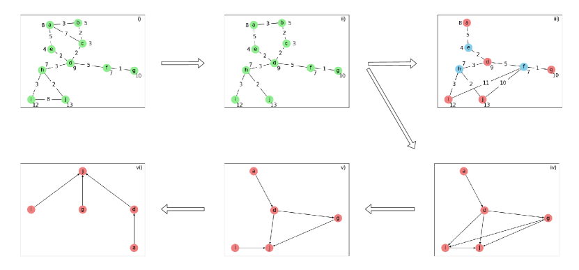
Figure 1: Generating the mountain graph and the line parent tree. In i), a graph is displayed with the heights next to the nodes and with the edge weight put in the middle of each edge. The RNG in ii) is derived by discarding the edge between i and j, because h is closer to both i and j than they are to each other and by discarding the edge between a and c because node b is closer to both of them than they are to each other. From this, the Mountain Graph is derived in iii), where we display the shortest path distances between the cols and peaks. Additionally, we derive from ii) the Peak Graph which is displayed in iv). According to Definition 8, we then discard the edge from g to i because j is closer to the key col f than i and we discard the edge between d and i because j is closer to the key col h to arrive at v). From this, the line parent tree vi) is derived by discarding the edge between d and g because the key col h over which j is reached is closer to g than the key col f over which g is reached.

In the following, we will work with undirected graphs $G=(V,E)$, where $E\subseteq\binom{V}{2}$. We call a function $w\colon E\to\mathbb{R}_{>0}$ a weighting function of $(V,E)$. If we have a triple $G=(V,e,w)$ where $(V,E)$ is an undirected graph and $w$ a weighting function on $(V,E)$, we call $G$ a weighted graph. If we simply speak of graphs, we refer to undirected and unweighted graphs.

A walk $p$ of a graph $G$ is a finite sequence $p=(v_{i})_{i=0}^{n}$ with $v_{i}\in V$ for all $i\in\{0,\dots n\}$ and $\{v_{j-1},v_{j}\}\in E$ for all $j\in\{1,\dots,n\}$. We call a walk $p$ a path, if for all $i\neq j$ it holds that $v_{i}\neq v_{j}$ or $\{i,j\}=\{1,n\}$. For each walk $p=(v)_{i=0}^{n}$, we call $\operatorname{start}(p)\coloneqq v_{0}$ the starting point and $\operatorname{end}(p)\coloneqq v_{n}$ the end point of $p$. We follow the usual convention to not distinguish between walks $p=(v_{i})_{i=0}^{n}$ and the corresponding set $\{v_{i}~{}|~{}i\in\{0,\dots n\}\}$, meaning that we say that $v$ is element of $p$ and write $v\in p$. A graph is connected, if for all pairs $u,v\in V$ there is a walk from $u$ to $v$. Additionally, let $N_{G}(v)\coloneqq\{u\in V~{}|~{}\{u,v\}\in E\}$ be the neighborhood of $v$ in $G$. If clear from the context, we omit $G$ and write $N(v)$.

We consider graphs with a height function $h\colon V\to\mathbb{R}_{\geq 0}$ and a metric, i.e., $d\colon V\times V\to\mathbb{R}_{\geq 0}$ with $\bullet$ $\forall x,y\in V:d(x,y)=0\iff x=y$(reflexivity), $\bullet$ $\forall x,y\in V:d(x,y)=d(y,x)$(symmetry) and $\bullet$ $\forall x,y,z\in V:d(x,z)\leq d(x,y)+d(y,z)$(triangle inequality).

Definition 1 (Landscape)

We call $L=(G,d,h)$ a landscape if $G=(V,E)$ is a connected and finite graph, $d$ is a metric on $V$ and $h$ is a height function on $V$ such that $h$ has a unique maximum. We denote the highest point by $\max(L)$.

To sum up, a landscape is given by a set of points, where we can traverse the points (via the given graph structure), where we know, how “high” each point is and where we can measure distances. If $G$ has a weighting function $w$ on it, a metric on the nodes of $G$ is provided by the weighted shortest path distance.

As mentioned earlier, our aim is to display hierarchies of peaks and connections between peaks and cols. For this, we first have to define peaks and cols. In the following, we will always assume to have given a landscape $L=(G,d,h)$.

Definition 2 (Peaks, Mountain paths and Cols)

We call a node $v\in V$ a peak of $L$ if $h(v)>h(u)$ for all $u\in N(v)$ and denote by $P(L)$ the set of peaks of $L$. A path $p$ of $G$ is a mountain path if $\operatorname{start}(p),\operatorname{end}(p)\in P(L)$. We denote by $M(L)$ the set of all mountain paths. For each $p\in M(L)$ we call $c(p)\coloneqq\operatorname{argmin}_{v\in p}h(p)$ the col of $p$. If this argmin is not unique, we choose the point in the path which is visited first.

To compute the prominence of a peak, we have to identify the cols which connect it with higher peaks.

Definition 3 (Cols of Peaks)

For each peak $v\in P(L)\setminus\{\max(L)\}$ we call the set $\uparrow_{L}(v)\coloneqq\{p\in M(L)~{}|~{}\operatorname{start}(p)=v,h(\operatorname{end}(p))>h(v),\not\exists u\in p\setminus\{\operatorname{end}(p),v\}:u\in P(L)\land h(u)>h(v)\}$ the ascending paths of $v$ and denote by $C_{L}(v)\coloneqq\{c(p)~{}|~{}p\in\uparrow_{L}(v)\}$ the set of all cols of $v$.

To sum up, the ascending paths $p\in\uparrow_{L}(v)$ are the paths from $v$ to higher peaks such that there is no higher peak $w\in p$ and the cols of $v$ are the lowest points of the ascending paths We omit the $L$ in the index if clear from the context. As prominence for mountain peaks is the minimal descent needed to go to higher points, we are just interested in the highest cols.

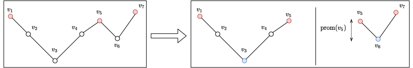
Figure 2: Prominence: Here, the vertical positioning displays the height of the different points. To compute the prominence of $v_{5}$, we first identify the paths that lead to higher peaks. Then, we determine the cols of these paths and compute the height difference of $v_{5}$ to these cols. The lower difference yield the prominence of $v_{5}$.

Definition 4 (Key Cols and Prominence)

Let $\operatorname{prom}_{L}(\max(L))\coloneqq h(\max(L))$. For each peak $v\in P(L)\setminus\{\max(L)\}$ we call the elements of $K_{L}(v)\coloneqq\{u\in C_{L}(v)~{}|~{}h(u)=\max_{\tilde{u}\in C_{L}(v)}h(\tilde{u})\}$ the key cols of $v$. For $u\in K_{L}(v)$ the prominence of $v$ is given via

$$\operatorname{prom}_{L}(v)\coloneqq h(v)-h(u).$$

Thus, the prominence of a peak $v$ displays the vertical distance to the key cols. For $v\in P(L)\setminus\{\max(L)\}$ the prominence is the minimal height difference to a col, i.e., $\operatorname{prom}_{L}(v)=\min_{u\in C(v)}h(v)-h(u).$ Again, we write $\operatorname{prom}(v)$ and $K(v)$ if the choice of the landscape is clear. An illustration of the definition of prominence is given by Figure 2.

We are interested in the structure which determines the prominence of peaks, i.e., in the higher peaks to reach from a specific peak and in the cols which connects the peaks of the mountain landscape. Hence, we do not only study the key cols of peaks but also the higher peaks that can be reached from their cols.

Definition 5 (Dominators)

Let $v$ be a peak of the landscape $L$. We then call the set $D_{L}(v)\coloneqq\{\operatorname{end}(p)~{}|~{}p\in\uparrow_{L}(v)\land c(p)\in K(v)\}$ the dominators of $v$.

Definition 6 (Mountain Graph)

For a given landscape $L=((V,E),d,h)$, let $K(L)\coloneqq\cup_{v\in P(L)}K_{L}(v)$ be the set of key cols of L and let $V_{\operatorname{MG}}(L)\coloneqq P(L)\cup K(L)$ be the critical points of $L$. Let for $v\in P(L)$ be $\uparrow_{L}^{K}\!(v)\coloneqq\{p\in\uparrow_{L}\!(v)~{}|~{}c(p)\in K_{L}(v)\}$ the ascending paths of $v$ with key cols as cols. Let then

$$E_{\operatorname{MG}}(L)\coloneqq\bigcup_{v\in P(L)}\left(\bigcup_{p\in\uparrow_{L}^{K}\!(v)}\{\{v,c(p)\},\{c(p),\operatorname{end}(p)\}\}\right).$$

The graph $\operatorname{MG}=(V_{\operatorname{MG}}(L),E_{\operatorname{MG}}(L))$ is called the mountain graph of $L$ and the landscape $L_{\operatorname{MG}}\coloneqq(\operatorname{MG}_{L},d|_{\operatorname{MG}},h|_{\operatorname{MG}})$ the mountain landscape of $L$.

To sum up, if a peak $v_{1}$ is connected via a key col $u$ to a higher peak $v_{2}$, we add edges between $v_{1}$ and $u$ and between $u$ and $v_{2}$ to the mountain graph. Thus, the mountain graph displays which peaks are connected through which key cols. If clear from the context, we omit $L$ and simply write $\operatorname{MG}=(V_{\operatorname{MG}},E_{\operatorname{MG}})$. The mountain graph contains all relevant information for the computation of prominence values as the following theorem shows.

Theorem 3.1

The following statements hold:

1. $\operatorname{MG}$ is connected.

2. $P(L)=P(L_{\operatorname{MG}})$

3. Consider for each peak $v\in P(L)\setminus\{\max(L)\}$ of $L$ the set $N^{\prime}_{\operatorname{MG}}(v)\coloneqq\{u\in N_{\operatorname{MG}}(v)~{}|~{}\exists v^{\prime}\in N_{\operatorname{MG}}(u):h(v^{\prime})>h(v)\}$. Then:

   $$u\in N^{\prime}_{\operatorname{MG}}(v)\Rightarrow\exists u^{\prime}\in C_{L}(v):h(u^{\prime})\geq h(u).$$

4. It holds for $v\in P(L)\setminus\{\max(L)\}$ that:

   $$\operatorname{prom}_{L}(v)=\min_{u\in N^{\prime}_{\operatorname{MG}}(v)}(h(v)-h(u)).$$

Theorem 3.1 shows that to study relations between cols and peaks that determine prominence values, it is sufficient to check the cols to which a peak is connected in the mountain graph. Note, that the key cols and the paths between peaks passing through them have to be determined to derive the mountain graph. Hence, Theorem 3.1 does not allow for a faster computation of prominence values. Instead, it provides a representation that can be used to observe important connections between peaks and cols.

3.2 Line Parent Trees

As the prominence of mountain peaks is computed by descending to key cols and then ascending to higher peaks, a hierarchy between peaks arises by the question to which higher peak one can traverse from a key col of a given peak.

Definition 7 (Peak Graph)

Let

$$E_{P}(L)\coloneqq\bigcup_{v\in P(L)}\{\{\operatorname{start}(p),\operatorname{end}(p)\}~{}|~{}p\in\uparrow_{L}^{K}\!(v)\}.$$

We call $\operatorname{PG}(L)\coloneqq(P(L),E_{P}(L))$ the peak graph of $L$ and we call

$$T_{\operatorname{PG}(L)}\coloneqq\{(\operatorname{start}(p),c(p),\operatorname{end}(p))~{}|~{}p\in\uparrow_{L}^{K}\!(v)\}$$

the defining triples of $\operatorname{PG}(L)$.

Peaks may be connected to different key cols and different higher peaks. To define a meaningful hierarchy on the peaks, we use the metric $d$ to determine a unique line parent for all peaks.

Definition 8 (Line Parents)

Let $T^{\prime}_{\operatorname{PG}}(L)\coloneqq\{(v,u,\tilde{v})\in T_{\operatorname{PG}}\mid\not\exists v^{\prime}:(v,u,v^{\prime})\in T_{\operatorname{PG}}\land(d(u,v^{\prime})<d(u,\tilde{v})\lor(d(u,v^{\prime})=d(u,\tilde{v})\land h(v^{\prime})>h(\tilde{v})))\}$. Let $E_{\operatorname{LP}}(L)\coloneqq\{\{v,\tilde{v}\}~{}|~{}\exists u:(v,u,\tilde{v})\in T^{\prime}_{\operatorname{PG}}(L)\land\not\exists u^{\prime},v^{\prime}:(v,u^{\prime},v^{\prime})\in T^{\prime}_{\operatorname{PG}}(L)\land d(v,u^{\prime})<d(v,u)\}$. We call $\operatorname{LP}(L)\coloneqq(P(L),E_{\operatorname{LP}}(L))$ the line parent graph of $L$. If $\{u,v\}\in E_{\operatorname{LP}}(L)$ with $h(v)>h(u)$, $v$ is a line parent of $u$.

Again, we omit $L$ when possible without confusion. In Definition 8, we first remove edges to higher peaks that are further away from the corresponding key col. If there are multiple higher peaks with the exact same distance to the key col, we keep the highest peak. Then we remove edges where the key col is further away. If for all $v\in P(L)\setminus\max(L)$ the line parent is unique, $\operatorname{LP}(L)$ is a tree.

Theorem 3.2

If for each peak $v\in P(L)\setminus\{\max(L)\}$ the line parent is unique, then $\operatorname{LP}(L)$ is a tree.

The uniqueness of the line parent is only violated in two cases. First, if there are multiple peaks being reached after the same key col with the exactly same distance to the key and the same height. In such a case, we can enforce the uniqueness by sampling one of the peaks. Secondly, if there are key cols $c_{1},\dots,c_{n}$ with corresponding higher peaks $p_{1}\dots p_{n}$ with the exact same distance to the point. In such a case, we choose $p_{i}$ such that $d(c_{i},p_{i})$ is minimal. If these minimum is reached multiple times, we enforce uniqueness by sampling one of the higher peaks with minimal distance to the corresponding key col.

To sum up, we enforce the uniqueness of the line parent. The simple edge structure of trees enables a satisfactory visualization even for medium sized node sets. The line parent tree can also be used to study dominance relationships with a non peak as a starting point. In this case, we suggest to navigate through the line parent tree starting with the closest peak with respect to the given metric.

3.3 Discarding Edges via Relative Neighborhood Graphs

Let $G=(V,E,w)$ be a weighted graph and let $h\colon V\to\mathbb{R}_{\geq 0}$ be a height function on $G$. In the following, we extend this structure to a landscape by using the shortest path metric on $G$. In practical applications, the amount of peaks will often be very low. One reason for this is the huge amount of connections one may have in social networks. Let us for example assume to have a weighted co-follower graph (for example weighted with Jaccard-distance) where the height function is given by the amount of followers. Here, all pairs of users with just one common follower would be connected and thus nearly all users would have a “higher” neighbor and thus will not be peaks. Hence, it is of major interest to only keep edges which stand for a strong connection, i.e., edges between users with a large amount of common followers.

A straight-forward way to remove edges would be by choosing a $k\in\mathbb{N}$ and keep for all vertices only the $k$ edges with the smallest weights or to choose a $t\in(0,1)$ and remove all edges with weights higher than $t$. However, besides the disadvantage that in both cases a parameter has to be chosen, this procedure can lead to disconnected graphs. Restricting to the biggest connected component of the resulting graph would then lead to the discarding of whole regions of the graph. To this end, we develop in the following a parameter free, deterministic edge sampling approach which always preserves connectivity. This approach is based on the relative neighborhood graph (RNG) [26]. The RNG derives a graph structure from a metric space by connecting points nearby. More specifically, two points are connected if there is no third point which is closer to both of them.

Definition 9 (Relative Neighborhood Graph)

The relative neighborhood graph of a metric space $(M,d)$ is given by the undirected graph $\operatorname{RNG}(d)\coloneqq(M,E_{\operatorname{RNG}(d)})$ with $E_{\operatorname{RNG}(d)}\subseteq\binom{M}{2}$ such that $\{m_{1},m_{2}\}\in E_{\operatorname{RNG}(d)}$ if and only if there does not exist $m_{3}\in M$ with $\max(\{d(m_{1},m_{3}),d(m_{2},m_{3})\})<d(m1,m2)$.

Our goal is to thin out graphs by computing the RNGs. Hence, it is of fundamental interest that RNGs are connected. For points in $\mathbb{R}^{2}$, it has been shown that the RNG is a supergraph of the minimum-spanning-tree [26] which implies connectivity [8]. Because RNGs are commonly only studied in $\mathbb{R}^{d}$ with $L^{p}$ metrics we could not find a proof for the connectivity in arbitrary finite metric spaces. Hence, we prove it in the supplementary material.

Theorem 3.3 (Connectivity of relative neighborhood graph)

Let $(M,d)$ be a finite metric space. Then $\operatorname{RNG}(d)$ is connected.

What still needs to be shown is that deriving RNGs from the shortest-path metric is indeed an edge-reduction technique, i.e., that edges are just removed and that is not possible that new edges are added.

Theorem 3.4 (RNG as Edge-Reduction)

Let $G=(V,E,w)$ be a connected, undirected and weighted graph and $d_{\operatorname{SP}}:V\times V\to\mathbb{R}_{\geq 0}$ be the shortest path metric on $G$. Then it holds that $E_{\operatorname{RNG}(d_{\operatorname{SP}})}\subseteq E$.

In the following, we use the term relative neighborhood graph of $G$, denoted by $\operatorname{RNG}(G)$, which will always refer to the RNG with respect to the shortest-path-metric. A sketch of an edge-reduction on a graph is given as part of Figure 1.

For a weighted graph $G=(V,E,w)$ with a height function $h$, our standard procedure is to 1. compute the weighted shortest path metric $d_{\operatorname{SP}}$, 2. compute $\operatorname{RNG}(G)$, 3. derive from this the following landscape.

Definition 10 (Essential Landscape)

Let $h:V\to R_{\geq 0}$ be a height function on a graph $G=(V,E,w)$. Let $d_{\operatorname{SP}}$ be the weighted shortest path metric on $G$. We call

$$L(G,h)\coloneqq(\operatorname{RNG}(G),d_{\operatorname{SP}},h)$$

the (essential) landscape of $G$ and $\operatorname{MG}(G,h)\coloneqq\operatorname{MG}(L(G,h))$ the essential mountain graph of $G$. We call $\operatorname{LP}(G,h)\coloneqq\operatorname{LP}(L(G,h))$ the (essential) line parent tree of $G$. If clear from the context, we simply write $\operatorname{MG}(G)$ and $\operatorname{LP}(G)$.

Complexity.

The naive approach to compute the RNG for a finite metric space $(M,d)$ would be to check for all pairs $m_{1}\neq m_{2}\in M$ whether there exists $m_{3}$ which is closer to both of them. This results in an algorithm with runtime $\mathcal{O}(|M|^{3})$ [26]. For $\mathbb{R}^{d}$ with a $l_{p}$ metric, there are algorithms with better runtime [26, 1, 7]. However, these results can not be applied to shortest path metrics. To compute $\operatorname{RNG}(G)$ for a graph $G=(V,E)$, we can use Theorem 3.4 to speed up the computation as we only have to check the elements of $E$ and not all node pairs. Hence, computing the RNG has complexity $\mathcal{O}(|E|||V|)$.

4 Line Parent Trees of Real-World Networks

Table 1: Network statistics. In the first table, we display from left to right: 1.) the number of vertices of the network, 2.) its density 3.) the density of the RNG 4.) the number of vertices of the mountain graph, 5.) the density of the mountain graph, 6.) the number of vertices in the line parent tree, 7.) its maximum width and 8.) its depth. In the second table, we show the node sizes and degrees of the sampled graphs serving a) as a comparison for discarding edges via the RNG procedure and b) for serving as a comparison for the mountain graph which is computed from the RNG. For the latter, we apply the sampling baselines on the RNG, not on the original network itself.

	$|V|$	$D_{G}$	$D_{\operatorname{RNG}(G)}$	$|V_{\operatorname{MG}}|$	$D_{\operatorname{MG}}$	$|V_{\operatorname{LP}}|$	$W_{\operatorname{LP}}$	$DP_{\operatorname{LP}}$
Twitter>10K	6635	.9958	.0005	1171	.1089	652	88	20
Twitter>100K	430	1.0000	.0064	146	.1084	84	14	13
ECML/PKDD	742	.0123	.0052	190	.1957	98	21	10
KDD	1674	.0100	.0036	219	.2236	115	30	8
PAKDD	889	.0124	.0054	132	.2155	67	27	5

	$\operatorname{RNG}$ Baselines				$\operatorname{MG}$ Baselines
	ES		CNARW[16]		RPN[12]		RCMH[15]
	$|V|$	$D_{G}$	$|V|$	$D_{G}$	$|V|$	$D_{G}$	$|V|$	$D_{G}$
Twitter>10K	5192.8	.0008	5174	.0007	271.1	.0079	1171	.0021
Twitter>100K	374.8	.0084	325.5	.0112	35.9	.0652	146	.0168
ECML/PKDD	650.7	.0067	560	.0092	77.1	.0304	190	.0153
KDD	1575.5	.0041	1407.5	.0041	67.2	.0390	219	.0138
PAKDD	814.7	.0064	704.1	.0087	34.3	.0812	132	.0222

We experiment with networks built from a Twitter follower network [11, 3, 4] which we found at SNAP [13] and with networks that display co-author relations. These networks are derived from the Semantic Scholar Open Research Corpus [2]. From the Twitter dataset, we derive two weighted co-follower networks. In these networks two users have an edge if they have a common follower. The edges are weighted via Jaccard distance. We derive a version containing users with at least $10,000$ followers (Twitter>10K) and a network containing users with at least $100,000$ followers (Twitter>100K). Here, the height of a user is given via the amount of followers.

The co-author networks are derived by considering communities of authors that regularly publish at a specific conference. We derive datasets for the European Conference on Machine Learning and Principles and Practice of Knowledge Discovery in Databases (ECML/PKDD), the SIGKDD Conference on Knowledge Discovery and Data Mining (KDD) and the Pacific-Asia Conference on Knowledge Discovery and Data Mining (PAKDD). The heights of the authors are given via h-indices.

For all graphs, we use well-established measures to get further insights into our notions. To be more detailed, we display node sizes and densities of the networks themselves, the RNGs and the mountain graphs derived from the RNGs. Additionally, we display node sizes, maximum widths and depths of the line-parent trees derived from the RNGs. The results can be found in Table 1. Plots of all labeled trees and details on dataset creation are part of the supplementary material.

4.1 Comparison with Sampling Approaches

To further understand the steps of our approach, we compare them with commonly used sampling approaches [16, 12, 15]. To be more specific, we sample edges from the original network to get graphs which have an equal amount of edges as the RNG. Then we take the biggest connected component of these graphs. We call these methods the RNG Baselines. We use two sampling approaches: First, we sample edges with the probability of an edge e to be chosen being proportional to $1-w(e)$, where $w(e)$ is the weight of the edge. We call the resulting baseline the Edge Sampling (ES) approach. As a second comparison, we use a weighted version of CNARW [16], a modern random walk approach.

Additionally, we use sampling approaches to sample from the RNG in such a way, that we have an equal amount of nodes as in the mountain graph and take the biggest component of the resulting network. We call these methods the MG Baseline. First, we sample nodes by their PageRank value viaRPN [12]. Again, we also use a modern random walk based approach, namely RCMH [15]. The CNARW method used above relies on common neighbors. Since triangles in the RNG are very uncommon (for these, 2 of the 3 corresponding edges in the original graph need to have the same distance weight), we use RCMH instead.

Note, that we use the comparison with other methods to contextualize our novel structures. As our structures have a different purpose, namely displaying important connections that are derived from the original network, they are not directly comparable to regular sampling approaches. These approaches derive small graphs that behave similar to the original graph with respect to specific measures. This makes it unreasonable to interpret the comparison to our baselines as a competition where higher/lower node sizes or densities are, in some way, better. As our comparison methods include random sources, we repeat them 10 times and report means. Statistics, including sizes of the derived RNGs, mountain graphs and line parent trees, can be found in Table 1. Additionally, we include node sizes and densities for all comparison approaches.

We observe that computing the RNG reduces the density by a large margin. It stands out, that this effect is stronger for the dense Twitter networks. When sampling an equal amount of edges, there are nodes which do not belong to the biggest connected component anymore. This results in a higher density of the (biggest component) of the networks created by sampling compared to the RNG.

The resulting line parent trees are much smaller than the original network, reducing the node set by a factor of about $5$ to $10$ times. Another remarkable point is that the mountain graph is always denser than the RNG from which it is computed and than the graphs which are sampled via the comparison methods. An explanation is that edges from a peak $v$ to a col $u$ in the mountain graph correspond to paths (not edges!) in the RNG. As the amount of paths in a graph is commonly remarkably higher than the amount of edges, this could be one reason for the higher density of the mountain graph.

4.2 Distances to Line-Parent Trees

Table 2: Mean, median and maximum of the minimal shortest path distance (MSPD) from all non-peaks $v$ to the set $P$ of all peaks (left) to the set $H$ which contains the $|P|$ highest nodes of the network (right).

	$d(P)_{\text{Mean}}$	$d(P)_{\text{Median}}$	$d(P)_{\text{Max}}$	$d(H)_{\text{Mean}}$	$d(H)_{\text{Median}}$	$d(H)_{\text{Max}}$
Twitter>10K	0.87	0.88	1.00	0.90	0.91	1.00
Twitter>100k	0.86	0.87	0.97	0.92	0.95	0.99
ECML	1.28	1.00	2.98	1.74	1.91	4.91
KDD	1.30	1.00	2.95	1.83	1.95	3.90
PAKDD	1.46	1.00	3.78	1.94	1.96	4.90

To investigate to which extent line parent trees are representative for the structure of the whole network, we compute how “dense” the line parent trees lay in the networks, i. e. the shortest path lengths from all non-peaks to the peaks. To evaluate whether choosing locally outstanding nodes lead to a better representation than choosing nodes solely based on their height, we compare our approach with a “naive” approach of assuming the $n$ highest points to be relevant, where $n$ is the amount of peaks. To be more detailed, we compute for each non-peak $v$ the minimal shortest path distances (MSPD) to all peaks in the original graph $G$. We do the same using the $n$ highest points instead of the set of peaks. We report means, medians and maximum values over the MSPDs of all non-peaks, the results can be found in Table 2.

Our results show that locally outstanding nodes better reflect the overall network then just choosing the highest nodes, with median and mean values of the MSPDs being fundamentally lower. Furthermore, median MSPDs to peaks are always not higher then $1$. In contrast, MSPDs to the “highest” nodes have median values of nearly $2$ for the sparse co-author networks. This indicates that selecting locally outstanding points indeed lead to a more reasonable representation instead of selecting nodes solely by their hight, ignoring spatial information. Note, that we compute distances in a weighted graph. Hence, shortest path distances (and thus medians and maxima over them) do not have to be integers.

5 Experiments on Random Data

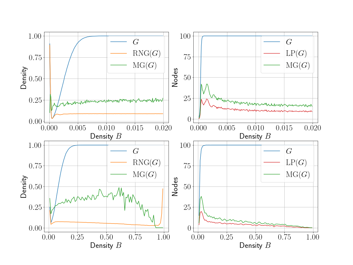
Figure 3: Experiments on random data. In both rows, the set $M_{1}$ on which is projected has size $100$. The other set has size $100,000$ on the first row and size $100$ in the second row. The x-axes display the densities of the original bipartite graph $B$. The left plots display the densities for the resulting network $G$, which is the biggest connected component of the weighted projection, the line parent tree $\operatorname{RNG}(G)$ and the mountain graph $\operatorname{MG}(G)$. The right pictures plot the node size of $G,\operatorname{MG}(G)$ and $\operatorname{LP}(G)$.

To investigate sizes and densities of the RNG, the mountain graph and the line parent tree, we additionally experiment with randomly generated data. Here, we start with a randomly generated bipartite graph with vertex sets $M_{1},M_{2}$ with $|M_{1}|=100$ and $|M_{2}|\in\{100000,100\}$. We then project on the vertex set $M_{1}$ and set for two vertices with an edge in the resulting graph the edge weight to the Jaccard distance. The graph $G$ is then given via the biggest connected component of this graph. As height function, we map each vertex to the amount of neighbors in the original bipartite network. This procedure is motivated by the background of often investigated real-world networks. Co-author networks are for example projection from the bipartite author-publication graph. Here, the corresponding height function then would be the amount of papers of an author, where each author is connected to multiple publications but only a small amount of the overall publications. This leads to a small density of the bipartite network.

We generate networks for different densities $d$. Namely, we iterate $d$ through $\{0.0001,0.0002,\dots,0.01999\}$ for $|M_{2}|=100,000$ and through $\{0.01,0.02,\dots 0.99\}$ for $|M_{2}|=100$. The experiments with different sizes of $|M_{2}|$ allow us to investigate if our methods behave fundamentally different for networks of different kinds. From $G$ we compute the $\operatorname{RNG}(G)$, the mountain graph $\operatorname{MG}(G)$ and the line parent hierarchy $\operatorname{LP}(G))$ of the essential landscape. For each $d$ and $|M_{2}|$, we repeat this procedure 20 times and display means. The results can be found in Figure 3. The following facts stand out.

• The density of both the $\operatorname{RNG}$ and the mountain graph of the $\operatorname{RNG}$ are growing in a significant smaller pace than the density of $G$. Considering the case $|M_{2}|=100,000$ it is remarkable, that, when $G$ has a density of nearly $1$, the density of both other graphs are still under $0.3$.

• The characteristic points for describing the resulting mountain landscape build indeed a subset that is remarkably smaller than the vertex size of the biggest component of $G$.

• Considering the second row, it stands out that for very high densities of nearly $1$ of the original bipartite network, the density and thus the amount of edges of the RNG start to rise rapidly. We assume that this is driven by the case, that, if the bipartite graph is nearly complete, there will be a large amount of vertex pairs with the same neighbor set in the bipartite graph. Thus, nearly all shortest path distances are equal and just very few edges will be discarded. In consequence, the mountain graph is built from a nearly complete graph where nearly all edges have similar weights. Thus, there will be only a small amount of peaks and the mountain graph is nearly vanishing.

Note, that we use a height function that is directly derived from the graph. Such height functions are indeed reasonable. For example, the amount of followers of Twitter users in co-follower graphs is indeed a useful indicator of their importance.

6 Conclusion and Future Work

In this work, we showed how the notions of peaks, cols and line parents, which are originally designed to characterize connections and hierarchies between mountains, can be adapted to networks. We discussed how these notions can be used to identify important vertices and meaningful connections and hierarchies between them. Our method further benefits from a novel preprocessing procedure that removes unimportant edges without hurting the connectivity of the network. This preprocessing step is based on relative neighborhood graphs which were originally invented to connect data points in two-dimensional euclidean spaces.

Our experiments indicate that our method finds dependencies and hierarchies from the original network that are remarkably smaller than the original graph and therefore can enhance the comprehension of real-world social networks.

Future work will investigate the application to further kinds of networks such as friendship networks on Facebook. As some of these networks may be unweighted, the question arises on how to use our RNG procedure in this case. On the other hand, it would be interesting to involve temporal aspects in networks. How does the line parent hierarchy of social networks change over time?

References

- [1] Agarwal, P.K., Matousek, J.: Relative neighborhood graphs in three dimensions. In: Ann. Symp. on Discrete Algorithms (1992)
- [2] Ammar, W., Groeneveld, D., Bhagavatula, C., Beltagy, I., Crawford, M., Downey, D., Dunkelberger, J., Elgohary, A., Feldman, S., Ha, V., Kinney, R., Kohlmeier, S., Lo, K., Murray, T., Ooi, H., Peters, M.E., Power, J., Skjonsberg, S., Wang, L.L., Wilhelm, C., Yuan, Z., van Zuylen, M., Etzioni, O.: Construction of the literature graph in semantic scholar. In: NAACL (2018)
- [3] Boldi, P., Rosa, M., Santini, M., Vigna, S.: Layered label propagation: a multiresolution coordinate-free ordering for compressing social networks. In: WWW (2011)
- [4] Boldi, P., Vigna, S.: The webgraph framework I: compression techniques. In: WWW (2004)
- [5] Clauset, A., Moore, C., Newman, M.E.: Hierarchical structure and the prediction of missing links in networks. Nature (2008)
- [6] Gupte, M., Shankar, P., Li, J., Muthukrishnan, S., Iftode, L.: Finding hierarchy in directed online social networks. In: WWW (2011)
- [7] Jaromczyk, J.W., Kowaluk, M.: A note on relative neighborhood graphs. In: Ann. Symp. on Computational Geometry, Waterloo (1987)
- [8] Jaromczyk, J.W., Toussaint, G.T.: Relative neighborhood graphs and their relatives. Proceedings of the IEEE (1992)
- [9] Karatzoglou, A.: Applying topographic features for identifying speed patterns using the example of critical driving. In: ACM SIGSPATIAL International Workshop on Computational Transportation Science (2020)
- [10] Krishnamurthy, V., Sun, J., Faloutsos, M., Tauro, S.L.: Sampling internet topologies: How small can we go? In: International Conference on Internet Computing (2003)
- [11] Kwak, H., Lee, C., Park, H., Moon, S.B.: What is twitter, a social network or a news media? In: WWW (2010)
- [12] Leskovec, J., Faloutsos, C.: Sampling from large graphs. In: KDD (2006)
- [13] Leskovec, J., Krevl, A.: SNAP Datasets: Stanford large network dataset collection. http://snap.stanford.edu/data (2014)
- [14] Li, F., Zou, Z., Li, J., Li, Y.: Graph compression with stars. In: PAKDD (2019)
- [15] Li, R., Yu, J.X., Qin, L., Mao, R., Jin, T.: On random walk based graph sampling. In: IEEE International Conference on Data Engineering (2015)
- [16] Li, Y., and2 Shuai Lin, Z.W., Xie, H., Lv, M., Xu, Y., Lui, J.C.S.: Walking with perception: Efficient random walk sampling via common neighbor awareness. In: IEEE International Conference on Data Engineering (2019)
- [17] Lu, C., Yu, J.X., Li, R., Wei, H.: Exploring hierarchies in online social networks. IEEE Trans. Knowl. Data Eng. (2016)
- [18] Maiya, A.S., Berger-Wolf, T.Y.: Inferring the maximum likelihood hierarchy in social networks. In: IEEE International Conference on Computational Science and Engineering (2009)
- [19] Nelson, G.D., McKeon, R.: Peaks of people: using topographic prominence as a method for determining the ranked significance of population centers. The Professional Geographer (2019)
- [20] Pavlík, J.: Topographic spaces over ordered monoids. Math. Appl (2015)
- [21] Rafiei, D., Curial, S.: Effectively visualizing large networks through sampling. In: IEEE Visualization Conference (2005)
- [22] Royer, L., Reimann, M., Andreopoulos, B., Schroeder, M.: Unraveling protein networks with power graph analysis. PLoS computational biology (2008)
- [23] Schmidt, A., Stumme, G.: Prominence and dominance in networks. In: EKAW (2018)
- [24] Stubbemann, M., Hanika, T., Stumme, G.: Orometric methods in bounded metric data. In: IDA (2020)
- [25] Toivonen, H., Zhou, F., Hartikainen, A., Hinkka, A.: Compression of weighted graphs. In: KDD (2011)
- [26] Toussaint, G.T.: The relative neighbourhood graph of a finite planar set. Pattern Recognition (1980)