A Closer Look at Reference Learning
for Fourier Phase Retrieval

Abstract

Reconstructing images from their Fourier magnitude measurements is a problem that often arises in different research areas. This process is also referred to as phase retrieval. In this work, we consider a modified version of the phase retrieval problem, which allows for a reference image to be added onto the image before the Fourier magnitudes are measured. We analyze an unrolled Gerchberg-Saxton (GS) algorithm that can be used to learn a good reference image from a dataset. Furthermore, we take a closer look at the learned reference images and propose a simple and efficient heuristic to construct reference images that, in some cases, yields reconstructions of comparable quality as approaches that learn references. Our code is available at https://github.com/tuelwer/reference-learning.

1 Introduction

In general, Fourier phase retrieval is the problem of reconstructing an image from its Fourier magnitude measurements. The problem arises in different research areas, e.g., in X-ray crystallography [11], astronomical imaging [3], optics [15], array imaging [1], or microscopy [17]. In particular, for non-oversampled measurements, phase retrieval has not been fully solved yet. In this work, a slightly modified version of the problem is considered: instead of reconstructing the image from the plain magnitude measurements, a reference image is added onto the original image before the Fourier magnitudes are measured, i.e., we reconstruct the image $x\in\mathbb{R}^{d\times d}$ from the modified measurements

$$y=|\mathcal{F}(x+u)|,$$ (1)

where $\mathcal{F}$ denotes the discrete two-dimensional Fourier transform and $u\in\mathbb{R}^{d\times d}$ is a known reference image. Furthermore, we assume that both the image and the reference are non-negative. Figure 1 gives an overview of the measurement process, that can also be implemented in practice.

Figure 1: An overview of the measurement process with a known reference.

2 Related Work and our Contributions

The modified phase retrieval problem was first analyzed by Kim and Hayes [7, 6]. Recently, Hyder et al. [5] showed that such a reference can be learned from a rather small dataset using an unrolled gradient descent algorithm. While it is interesting that this is possible, a couple of questions arise which we discuss in this work.

Our Contributions:

1. We modify the well-established Gerchberg-Saxton (GS) algorithm [4] so that it utilizes a reference. Furthermore, we show that this modified GS algorithm can be unrolled to learn a reference image (similar to the approach of Hyder et al. [5]).

2. We answer the question under which conditions learning a reference image for Fourier phase retrieval is really necessary. For this, we propose a simple baseline reference image that is easily constructed and compare its performance with the learned references in the oversampled and the non-oversampled case.

The idea of unrolling algorithms has been considered before for other phase retrieval problems: The performance of an unrolled GS algorithm for phase retrieval has been analyzed by Schlieder et al. [14]. Naimipour et al. [12] unrolled the Wirtinger flow algorithm for compressive phase retrieval. Unlike our work, these papers augment existing phase retrieval algorithms with learnable parameters which is different from the reference based phase retrieval we consider in this work.

3 Unrolling the Gerchberg-Saxton Algorithm to Learn a Reference

The phase retrieval algorithm discussed in Hyder et al. [5] is a gradient descent method that requires extensive parameter tuning of its step size. For this reason, we unroll the GS algorithm, which typically converges within a few iterations. The GS algorithm iteratively replaces the magnitude of the current estimate with the measured magnitude and enforces a positivity-constraint on the image after the reference has been subtracted. Algorithm 1 shows our modified version of GS that utilizes a reference image. We learn the reference by calculating the mean squared error (MSE) between outputs of the GS algorithm after $n$ iterations and the corresponding original images. Then we perform backpropagation to calculate the gradient with respect to the reference $u$ and update it using a gradient descent step. These steps are repeated for multiple batches until convergence is achieved.

Input: Fourier magnitude $y\in\mathbb{R}^{d\times d}$, reference image $u\in\mathbb{R}^{d\times d}$, initialization $x_{0}\in\mathbb{R}^{d\times d}$, number of iterations $n$

Output: Reconstruction $x_{n}\in\mathbb{R}^{d\times d}$

1 for $k=1,\dots,n-1$ do

       $p_{k+1}\leftarrow\mathcal{F}(x_{k}+u)/|\mathcal{F}(x_{k}+u)|$

        // Estimate phase

2      

      $\bar{x}_{k+1}\leftarrow\mathcal{F}^{-1}(p_{k+1}\odot y)-u$

        // Fourier constraints and subtract u

3      

      $x_{k+1}\leftarrow\max(0,\bar{x}_{k+1})$

        // Image constraints (max is element-wise)

4      

5 end for

return $x_{n}$

Algorithm 1 Gerchberg-Saxton algorithm for phase retrieval with a reference image

4 Constructing Simple References Mimicking the Learned Ones

Learned ref. from Hyder et al. [5]	Learned ref. for GS (ours)	Simple ref. (ours)

Figure 2: Comparison of different learned references. For each of the two learned methods, the shown references are trained on the following datasest: MNIST, EMNIST, FMNIST, SVHN, CIFAR-10. Our simple reference is shown on the right.

Learning the reference image is computationally expensive. The most obvious baseline reference is a random image. For this, we sample the pixel values from a uniform distribution $\mathcal{U}(0,1)$. Looking at various learned reference images produced by the algorithm of Hyder et al. [5] and our unrolled GS algorithm (Figure 2), we see that most pixels are either zero or one. This suggests to also consider random binarized reference images.

However, looking more closely at those learned reference images (Figure 2), we see that all references exhibit flat areas. Furthermore, the learned references do not show any symmetries. These observations suggest trying a simple reference image as a baseline mimicking those features. To construct such a reference, we start with a black image that has a white square in the bottom right corner. After blurring this image with a Gaussian filter, we normalize and add weighted Poisson noise to every pixel. Finally, we binarize the image appropriately. A resulting simple reference is shown on the right in Figure 2.

In the next section, we compare the performance of these different references for reconstructing images from their oversampled and non-oversampled magnitude measurements.

5 Comparing Baseline and Learned References

Experimental Setup.

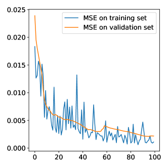
Figure 3: Training and validation MSE between reconstructions and original images of the FMNIST dataset.

To study whether references are necessary at all, we also reconstruct images from measurements that were taken without adding a reference onto the image. In that case, the trivial ambiguities (translation and flip) cannot be resolved by the reconstruction algorithm. Therefore, we register the reconstructions appropriately before calculating the error. For fair comparison, we register the reconstructions of the other methods before calculating the MSE as well.

We evaluate the reconstructions of images from the MNIST [10], the EMNIST [2], the FMNIST [16], the SVHN [13], and the CIFAR-10 [9] datasets. We convert the images from the SVHN and the CIFAR-10 dataset to grayscale. We consider non-oversampled magnitude measurements as well as measurements that are oversampled by a factor of two in each dimension. To solve the Fourier phase retrieval problem, we use a similar algorithm as Hyder et al. [5]. We run the algorithm for $500$ steps and set the step size to $\alpha=1.95$, which was chosen on a validation dataset. For each of the datasets, we use $1000$ images for testing and we train the references on $100$ training images using Adam [8] with a learning rate of $0.01$. We use batches of size $10$. During training, we unroll the GS algorithm for $15$ steps and use $500$ steps to reconstruct the images at test time.

Similar to the intensities of the images, we restrict the entries of the reference image to lie between $0$ and $1$ as using larger values makes the problem trivial to solve, i.e., even a random reference with values between $0$ and $100$ yields perfect reconstructions.

Results.

	Method	MNIST	EMNIST	FMNIST	SVHN	CIFAR-10
Non-oversampled	No reference	0.035615	0.063414	0.042417	0.013985	0.035134
	Random ref.	0.052724	0.079784	0.046670	0.012393	0.030222
	Random ref. (binary)	0.055324	0.081130	0.049436	0.012447	0.029299
	Simple ref. (ours)	0.060027	0.089347	0.067549	0.011270	0.024128
	Hyder et al. [5]	0.002607	0.014687	0.013649	0.010131	0.024141
	Unrolled GS (ours)	0.002181	0.015427	0.019863	0.008775	0.020020
Oversampled	No reference	0.020566	0.032907	0.021068	0.007516	0.020518
	Random ref.	0.005350	0.025308	0.011484	0.003670	0.009848
	Random ref. (binary)	0.001170	0.010994	0.006842	0.002462	0.007310
	Simple ref. (ours)	0.000761	0.003681	0.000848	0.000187	0.000495
	Hyder et al. [5] ref.	0.000132	0.000023	0.000073	0.000126	0.001415
	Unrolled GS ref. (ours)	0.000071	0.000257	0.000055	0.000055	0.000125

Table 1: Comparison of the mean squared reconstruction error using different references for Fourier phase retrieval from non-oversampled and oversampled magnitudes. Best values are printed bold.

	No reference	Simple ref. (ours)	Hyder et al. [5] ref.	Unrolled GS ref. (ours)
Non-oversampled
Oversampled

Figure 4: Reconstructions of the MNIST, the FMNIST and the CIFAR-10 dataset from non-oversampled and oversampled Fourier magnitudes using different references.

Table 1 shows that our unrolled GS algorithm is able to learn references of similar quality as the method proposed by Hyder et al. [5]. We see that the reconstruction errors of our simple reference are quite close to the errors of the learned methods in the oversampled case. Figure 3 shows the training and the validation loss for a reference trained using our unrolled GS algorithm on the FMNIST dataset. We can observe that only a few stochastic gradient descent steps are necessary to drastically decrease training and validation error. Also, our GS algorithm requires only a small number of iterations in training to learn a good reference. Figure 4 visualizes some reconstructions. In the non-oversampled case, the learned references produce better reconstructions than our simple reference. Surprisingly, the random references that we use as baseline perform worse on the MNIST-like datasets than using no baseline in the non-oversampled case. In the oversampled case, the learned references, as well as our simple reference, produce almost perfect reconstructions. Therefore, we conclude that learning references is not necessary when the Fourier magnitudes are oversampled.

6 Conclusion

In this paper, we discuss how the GS algorithm can be unrolled in order to learn a reference image for phase retrieval. We show that our unrolled GS algorithm performs comparably to an existing method and requires only a few unrolling steps while having no hyperparameters that require extensive tuning. Furthermore, we provide a simple reference which puts the benefit of a learned reference into perspective, especially when oversampled magnitude measurements are available.

7 Broader Impact

Fourier phase retrieval is a fundamental and relevant imaging problem in many areas of science, e.g., in X-ray crystallography or microscopy. Ethical or societal consequences depend on the exact application of the phase retrieval algorithm. Our insights set the performance gain of learned reference images for phase retrieval into perspective. We propose a simpler and more efficient approach for reference construction which yields similar results and requires less computation and thus less energy.

References

- [1] Oliver Bunk, Ana Diaz, Franz Pfeiffer, Christian David, Bernd Schmitt, Dillip K Satapathy, and J Friso Van Der Veen. Diffractive imaging for periodic samples: retrieving one-dimensional concentration profiles across microfluidic channels. Acta Crystallographica Section A: Foundations of Crystallography, 63(4):306–314, 2007.
- [2] Gregory Cohen, Saeed Afshar, Jonathan Tapson, and Andre Van Schaik. Emnist: Extending mnist to handwritten letters. In 2017 International Joint Conference on Neural Networks (IJCNN), pages 2921–2926. IEEE, 2017.
- [3] James R Fienup and J Christopher Dainty. Phase retrieval and image reconstruction for astronomy. Image recovery: theory and application, 231:275, 1987.
- [4] Ralph W Gerchberg. A practical algorithm for the determination of phase from image and diffraction plane pictures. Optik, 35:237–246, 1972.
- [5] Rakib Hyder, Zikui Cai, and M Salman Asif. Solving phase retrieval with a learned reference. In European Conference on Computer Vision, pages 425–441. Springer, 2020.
- [6] Wooshik Kim and Monson H Hayes. Iterative phase retrieval using two fourier transform intensities. In International Conference on Acoustics, Speech, and Signal Processing, pages 1563–1566. IEEE, 1990.
- [7] Wooshik Kim and Monson H Hayes. Phase retrieval using two fourier-transform intensities. JOSA A, 7(3):441–449, 1990.
- [8] Diederik P Kingma and Jimmy Ba. Adam: A method for stochastic optimization. arXiv preprint arXiv:1412.6980, 2014.
- [9] Alex Krizhevsky et al. Learning multiple layers of features from tiny images. 2009.
- [10] Yann LeCun, Léon Bottou, Yoshua Bengio, and Patrick Haffner. Gradient-based learning applied to document recognition. Proceedings of the IEEE, 86(11):2278–2324, 1998.
- [11] Rick P Millane. Phase retrieval in crystallography and optics. JOSA A, 7(3):394–411, 1990.
- [12] Naveed Naimipour, Shahin Khobahi, and Mojtaba Soltanalian. Unfolded algorithms for deep phase retrieval. arXiv preprint arXiv:2012.11102, 2020.
- [13] Yuval Netzer, Tao Wang, Adam Coates, Alessandro Bissacco, Bo Wu, and Andrew Y Ng. Reading digits in natural images with unsupervised feature learning. NIPS Workshop on Deep Learning and Unsupervised Feature Learning, 2011.
- [14] Lennart Schlieder, Heiner Kremer, Valentin Volchkov, Kai Melde, Peer Fischer, and Bernhard Schölkopf. Learned residual gerchberg-saxton network for computer generated holography. 2020.
- [15] Adriaan Walther. The question of phase retrieval in optics. Optica Acta: International Journal of Optics, 10(1):41–49, 1963.
- [16] Han Xiao, Kashif Rasul, and Roland Vollgraf. Fashion-mnist: a novel image dataset for benchmarking machine learning algorithms. arXiv preprint arXiv:1708.07747, 2017.
- [17] Guoan Zheng, Roarke Horstmeyer, and Changhuei Yang. Wide-field, high-resolution fourier ptychographic microscopy. Nature photonics, 7(9):739, 2013.