A time-weighted metric for sets of trajectories to assess multi-object tracking algorithms

Abstract

This paper proposes a metric for sets of trajectories to evaluate multi-object tracking algorithms that includes time-weighted costs for localisation errors of properly detected targets, for false targets, missed targets and track switches. The proposed metric extends the metric in [1] by including weights to the costs associated to different time steps. The time-weighted costs increase the flexibility of the metric [1] to fit more applications and user preferences. We first introduce a metric based on multi-dimensional assignments, and then its linear programming relaxation, which is computable in polynomial time and is also a metric. The metrics can also be extended to metrics on random finite sets of trajectories to evaluate and rank algorithms across different scenarios, each with a ground truth set of trajectories.

I Introduction

Multiple object tracking (MOT) algorithms play a fundamental role in many applications, such as self-driving vehicles, robotics and surveillance [2]. In MOT, there is an unknown and time-varying number of objects that appear in the surveillance area, move following a certain trajectory and disappear from the surveillance area. This ground truth can therefore be represented as a set of trajectories [3]. The objective of MOT algorithms is to estimate this set of trajectories based on noisy sensor data. An important task is then to rank the performances of different algorithms by measuring how similar the estimated set of trajectories is to the ground truth [4].

The quantification of the error between the ground truth set of trajectories and the estimate is usually based on a distance function. For principled evaluation and an intuitive notion of error, it is desirable that this distance function is a metric in a mathematical sense [5]. In addition, we are interested in metrics that penalise the following important aspects of MOT: localisation errors for properly detected targets, the number of missed and false targets, and track switches [6, 7, 8].

For the related problem of multi-object filtering, in which we aim to estimate the set of targets at the current time step, the optimal subpattern assignment (OSPA) metric is widely used [9, 10]. However, this metric does not penalise missed and false targets, e.g., it can be insensitive to the addition of false targets, and it can promote algorithms with spooky effect at a distance [11]. The generalised OSPA (GOSPA) metric (with parameter $\alpha=2$) penalises localisation errors for properly detected targets, and the number of missed and false targets, as typically required in MOT performance evaluation [12]. In the GOSPA metric, we look for an optimal assignment between the targets in the ground truth and estimated targets, leaving missed and false targets unassigned.

For sets of trajectories, apart from penalising the errors for the estimated set of targets at each time step, we are usually interested in penalising track switches [6, Sec. 13.6]. That is, the optimal assignments between estimated trajectories and real trajectories may change at different time steps giving rise to undesired track switches. There are also a number of distance functions for sets of trajectories that are not metrics in the literature, for example, [13, 14, 15, 16, 17, 18, 19].

The OSPA⁽²⁾ metric is a OSPA metric with a specific base distance applied to sets of trajectories [20]. The OSPA⁽²⁾ metric establishes an assignment between real and estimated trajectories that is not allowed to change with time. This approach avoids track switching considerations and may not rank different estimated sets as desired in standard MOT performance evaluation, see Figure 1. As other metrics, OSPA⁽²⁾ can be applied by subsampling the set of trajectories at time steps of relevance [20, Sec. V.B.2]. In addition, for a single time step, OSPA⁽²⁾ becomes the OSPA metric for targets, which has the characteristics explained above.

(a) No localisation error, one track switch

(b) 4 missed and 4 false targets

Figure 1: Estimated set of trajectories $\mathbf{Y}=\{Y_{1},Y_{2}\}$ against the ground truth $\mathbf{X}=\{X_{1},X_{2}\}$. In (a), $\mathbf{Y}$ has zero localisation errors and a track switch. In (b), $\mathbf{Y}$ has zero localisation errors up to time step 3, but there are 4 missed and false targets at time steps 4 and 5 (Distance $\Delta_{1}$ may be arbitrarily large). OSPA⁽²⁾ penalises these two cases equally. With a low switching cost, according to the trajectory metrics [1], (a) has a lower error than (b).

Bento’s metrics [21] for sets of trajectories penalise track switches by first adding $\ast$-trajectories to the ground truth and the estimate so that both sets have equal cardinality. The track switches are penalised based on a track switching cost function that penalises changes in the permutations that associate the (augmented) estimated trajectories to the (augmented) true trajectories. A metric that extends the GOSPA metric to sets of trajectories and penalises the number of track switches based on changes in assignments/unassignments, without using permutations and $\ast$-trajectories, was proposed in [1]. The linear programming (LP) relaxation of this metric is also a metric and is computable in polynomial time [1]. We refer to these two metrics as trajectory metrics. These trajectory metrics penalise localisation errors for properly detected targets, and the number of missed, false targets, and track switches.

In this paper, we increase the flexibility of the trajectory metrics in [1] by adding time-weighted costs at each time step. This can be useful, for instance, in online tracking where we generally want to place more weight on estimates corresponding to recent time steps [18]. Time-weighted costs can also be useful to measure the accuracy of a prediction of the set of trajectories at future time steps, by placing more weight to closer time steps, similarly to the use of discounted costs in sensor management [22]. As in [1], the time-weighted trajectory metrics can also be extended to metrics on random finite sets (RFSs) of trajectories [3].

II Problem formulation and background

In the standard multi-object tracking model, there is an unknown number of objects at each time step in the surveillance area. Each object is born at a certain time step, moves following a certain sequence of states and dies [2]. An object trajectory is represented by a variable $X=\left(\omega,x^{1:\nu}\right)$ where $\omega$ is its initial time step, $\nu$ is its length and $x^{1:\nu}=\left(x^{1},...,x^{\nu}\right)$ is its sequence of consecutive states [3]. We consider trajectories from time step 1 to $T$, which implies that the variable $\left(\omega,\nu\right)$ belongs to the set $I_{(T)}=\left\{\left(\omega,\nu\right):1\leq\omega\leq T\,\mathrm{and}\,1\leq\nu\leq T-\omega+1\right\}$, and variable $X\in\mathbb{T}_{\left(T\right)}$ where $\mathbb{T}_{\left(T\right)}=\uplus_{\left(\omega,\nu\right)\in I_{(T)}}\left\{\omega\right\}\times\mathbb{R}^{\nu n_{x}}$ and $\uplus$ stands for the union of sets that are mutually disjoint.

The variable of interest in MOT is the (ground truth) set of trajectories up to time step $T$, which is denoted by $\mathbf{X}=\left\{X_{1},...,X_{n_{\mathbf{X}}}\right\}$. The set $\mathbf{X}$ belongs to $\Upsilon=\mathcal{F}\left(\mathbb{T}_{\left(T\right)}\right)$, which denotes the set of all finite subsets of $\mathbb{T}_{\left(T\right)}$.

Based on noisy sensor data, an MOT algorithm provides an estimated set of trajectories $\mathbf{Y}=\left\{Y_{1},...,Y_{n_{\mathbf{Y}}}\right\}$. We would like to measure the distance between $\mathbf{Y}$ and $\mathbf{X}$ to evaluate estimation error. A mathematically principled way of measuring distances is via metrics.

A metric on $\Upsilon$ is a function $d\left(\cdot,\cdot\right):\Upsilon\times\Upsilon\rightarrow\left[0,\infty\right)$ such that [5]

• $d\left(\mathbf{X},\mathbf{Y}\right)=0$ if and only if $\mathbf{X}=\mathbf{Y}$ (identity),

• $d\left(\mathbf{X},\mathbf{Y}\right)=d\left(\mathbf{Y},\mathbf{X}\right)$ (symmetry),

• $d\left(\mathbf{X},\mathbf{Y}\right)\leq d\left(\mathbf{X},\mathbf{Z}\right)+d\left(\mathbf{Z},\mathbf{Y}\right)$ (triangle inequality).

The aim of this paper is to propose a metric on the space $\Upsilon$. While the metric is designed for the space $\Upsilon$, which considers trajectories without holes, the proposed metric can also be used with trajectories with holes [1, Sec. II.A].

In most applications, the main aim of metrics is to rank different algorithms (each with a different $\mathbf{Y}$) against a ground truth set of trajectories (a single $\mathbf{X}$). The case in which we have a data set with several scenarios (each with a different ground truth) can be addressed via metrics on RFSs of trajectories, and will be explained in Section V.

II-A GOSPA metric

We review the GOSPA metric as it is a building block for the metric for sets of trajectories. Let us consider the sets of targets $\mathbf{x}=\left\{x_{1},...,x_{n_{\mathbf{x}}}\right\}$ and $\mathbf{y}=\left\{y_{1},...,y_{n_{\mathbf{y}}}\right\}$. We denote the set of all possible assignment sets between sets $\left\{1,..,n_{\mathbf{x}}\right\}$ and $\left\{1,...,n_{\mathbf{y}}\right\}$ as $\Gamma_{\mathbf{x},\mathbf{y}}$. That is, any set $\theta\in\Gamma_{\mathbf{x},\mathbf{y}}$ is such that $\theta\subseteq\left\{1,..,n_{\mathbf{x}}\right\}\times\left\{1,..,n_{\mathbf{y}}\right\}$ and, $\left(i,j\right),\left(i,j^{\prime}\right)\in\theta$ implies $j=j^{\prime}$ and, $\left(i,j\right),\left(i^{\prime},j\right)\in\theta$ implies $i=i^{\prime}$.

Definition 1.

Given a base metric $d_{b}\left(\cdot,\cdot\right)$ on $\mathbb{R}^{n_{x}}$, a scalar $c>0$, and a scalar $p$ with $1\leq p<\infty$, the GOSPA metric ($\alpha=2$) between sets of targets $\mathbf{x}$ and $\mathbf{y}$ is [12, Prop. 1]

$$d_{G}\left(\mathbf{x},\mathbf{y}\right)$$

$$=\min_{\theta\in\Gamma_{\mathbf{x},\mathbf{y}}}\left(\sum_{\left(i,j\right)\in\theta}d_{b}\left(x_{i},y_{j}\right)^{p}+\frac{c^{p}}{2}\left(\left|\mathbf{x}\right|+\left|\mathbf{y}\right|-2\left|\theta\right|\right)\right)^{1/p}.$$ (1)

where $\left|\mathbf{x}\right|$ denotes the number of elements in the set $\mathbf{x}$.

The first term in (1) corresponds to the localisation errors (to the $p$-th power) for assigned targets (properly detected targets), which meet $\left(i,j\right)\in\theta$. The terms $\frac{c^{p}}{2}\left(\left|\mathbf{x}\right|-\left|\theta\right|\right)$ and $\frac{c^{p}}{2}\left(\left|\mathbf{y}\right|-\left|\theta\right|\right)$ are the costs (to the $p$-th power) for missed and false targets, respectively. We have also dropped the dependence of $d_{G}\left(\cdot,\cdot\right)$ on $p$ and $c$ for notational simplicity.

In particular, the trajectory metrics use GOSPA with sets $\mathbf{x}$ and $\mathbf{y}$ with at most one element, such that $\left|\mathbf{x}\right|\leq 1$ and $\left|\mathbf{y}\right|\leq 1$. In this case, (1) becomes

$$d_{G}\left(\mathbf{x},\mathbf{y}\right) \triangleq\begin{cases}\min\left(c,d_{b}\left(x,y\right)\right)&\mathbf{x}=\left\{x\right\},\mathbf{y}=\left\{y\right\}\\ 0&\mathbf{x}=\mathbf{y}=\emptyset\\ \frac{c}{2^{1/p}}&\mathrm{otherwise.}\end{cases}$$ (2)

III Time-weighted trajectory metrics

This section presents the time-weighted trajectory metrics. Preliminary notation is introduced in Section III-A. The time-weighted multi-dimensional assignment and linear programming relaxation metrics are proposed in Sections III-B and III-C, respectively.

III-A Notation

We introduce the following notation to define the metrics. Given a single trajectory $X=\left(\omega,x^{1:\nu}\right)$, the set with the state of the trajectory at time step $k$ is

$$\tau^{k}\left(X\right)\triangleq\begin{cases}\{x^{k+1-\omega}\}&\omega\leq k\leq\omega+\nu-1\\ \emptyset&\text{otherwise}.\end{cases}$$ (3)

Similarly, given a set $\mathbf{X}$ of trajectories, the set $\tau^{k}\left(\mathbf{X}\right)$ of target states at time $k$ is

$$\tau^{k}\left(\mathbf{X}\right)=\bigcup_{X\in\mathbf{X}}\tau^{k}\left(X\right).$$ (4)

The sets of targets corresponding to trajectories $X_{i}$ and $Y_{j}$ at time step $k$ are denoted by $\mathbf{x}_{i}^{k}=\tau^{k}\left(X_{i}\right)$ and $\mathbf{y}_{j}^{k}=\tau^{k}\left(Y_{j}\right)$, respectively. These sets are such that $\left|\mathbf{x}_{i}^{k}\right|\leq 1$ and $\left|\mathbf{y}_{i}^{k}\right|\leq 1$.

In the trajectory metrics, there are assignments at a trajectory level to determine track switches. That is, at each time step, each target set $\mathbf{x}_{i}^{k}$ is assigned to a target set $\mathbf{y}_{i}^{k}$ or is left unassigned. The set of all possible assignment vectors between sets $\{1,\ldots,n_{\mathbf{X}}\}$ and $\{0,\ldots,n_{\mathbf{Y}}\}$ is denoted by $\Pi_{\mathbf{X},\mathbf{Y}}.$ The assignment vector $\pi^{k}=[\pi_{1}^{k},...,\pi_{n_{\mathbf{X}}}^{k}]\in\Pi_{\mathbf{X},\mathbf{Y}}$ meets $\pi_{i}^{k}\in\{0,\ldots,n_{\mathbf{X}}\}$ with the constraint that $\pi_{i}^{k}=\pi_{i^{\prime}}^{k}=j>0$ implies $i=i^{\prime}$. Here, $\pi_{i}^{k}=j\neq 0$ implies that $X_{i}$ is assigned to $Y_{j}$ at time $k$ and $\pi_{i}^{k}=0$ implies that $X_{i}$ is unassigned at time $k$. This definition of assignment vectors implies that, at a specific time step, there can only be one trajectory $Y_{j}$ assigned to a trajectory $X_{i}$, but multiple trajectories in $\mathbf{X}$ and $\mathbf{Y}$ can be left unassigned.

III-B Time-weighted multi-dimensional assignment metric

The proposed time-weighted metric based on multi-dimensional assignment is given by the following definition.

Definition 2.

For $1\leq p<\infty$, cut-off parameter $c>0$, switching penalty $\gamma>0$, base metric $d_{b}\left(\cdot,\cdot\right)$ in the single-target space, localisation time weight $w_{1}^{k}>0$ at time step $k$ and switching time weight $w_{2}^{k}>0$ at time step $k$, the time-weighted multi-dimensional assignment metric $d\left(\mathbf{X},\mathbf{Y}\right)$ between two sets $\mathbf{X}$ and $\mathbf{Y}$ of trajectories is

$$d\left(\mathbf{X},\mathbf{Y}\right) =\min_{\begin{subarray}{c}\pi^{k}\in\Pi_{\mathbf{X},\mathbf{Y}}\\ k=1,\ldots,T\end{subarray}}\left(\sum_{k=1}^{T}w_{1}^{k}d_{\mathbf{X},\mathbf{Y}}^{k}\left(\mathbf{X},\mathbf{Y},\pi^{k}\right)^{p}\right.$$

$$\>\left.+\sum_{k=1}^{T-1}w_{2}^{k}s_{\mathbf{X},\mathbf{Y}}\left(\pi^{k},\pi^{k+1}\right)^{p}\right)^{1/p}$$ (5)

where the costs (to the $p$-th power) for properly detected targets, missed targets and false targets at time step $k$ are

$$d_{\mathbf{X},\mathbf{Y}}^{k}\left(\mathbf{X},\mathbf{Y},\pi^{k}\right)^{p} =\sum_{\left(i,j\right)\in\theta^{k}\left(\pi^{k}\right)}d_{G}\left(\mathbf{x}_{i}^{k},\mathbf{y}_{j}^{k}\right)^{p}$$

$$+\frac{c^{p}}{2}\left(\left|\tau^{k}\left(\mathbf{X}\right)\right|+\left|\tau^{k}\left(\mathbf{Y}\right)\right|-2\left|\theta^{k}\left(\pi^{k}\right)\right|\right)$$ (6)

with

$$\theta^{k}\left(\pi^{k}\right) =\left\{(i,\pi_{i}^{k}):i\in\{1,\ldots,n_{\mathbf{X}}\},\vphantom{d\left(\mathbf{x}_{i}^{k},\mathbf{y}_{\pi_{i}^{k}}^{k}\right)}\right.$$

$$\,\left.\left|\mathbf{x}_{i}^{k}\right|=\left|\mathbf{y}_{\pi_{i}^{k}}^{k}\right|=1,\,d_{G}\left(\mathbf{x}_{i}^{k},\mathbf{y}_{\pi_{i}^{k}}^{k}\right)<c\right\}$$ (7)

and the switching cost (to the $p$-th power) from time step $k$ to $k+1$ is

$$s_{\mathbf{X},\mathbf{Y}}(\pi^{k},\pi^{k+1})^{p}=\gamma^{p}\sum_{i=1}^{n_{\mathbf{X}}}s\big{(}\pi_{i}^{k},\pi_{i}^{k+1}\big{)}$$ (8)

$$s\big{(}\pi_{i}^{k},\pi_{i}^{k+1}\big{)} =\begin{cases}0&\pi_{i}^{k}=\pi_{i}^{k+1}\\ 1&\pi_{i}^{k}\neq\pi_{i}^{k+1},\pi_{i}^{k}\neq 0,\pi_{i}^{k+1}\neq 0\\ \frac{1}{2}&\text{otherwise. \quad\quad\quad\quad\quad\quad\quad\quad}\end{cases}$$

In the metric (5), we have an assignment vector $\pi^{k}$ at a trajectory level at time step $k$. The change from $\pi^{k}$ to $\pi^{k+1}$ determines the switching cost (to the $p$-th power) in (8). If $\pi_{i}^{k}=\pi_{i}^{k+1}$, there is no switching cost for the $i$-th trajectory in the ground truth. If $\pi_{i}^{k}\neq\pi_{i}^{k+1}$ and both $\pi_{i}^{k}$ and $\pi_{i}^{k+1}$ are different from zero, which implies $X_{j}$ is assigned to two different trajectories in $\mathbf{Y}$ at time steps $k$ and $k+1$, the switching cost (to the $p$-th power) is $\gamma^{p}$. Finally, if $\pi_{i}^{k}\neq\pi_{i}^{k+1}$ and either $\pi_{i}^{k}$ or $\pi_{i}^{k+1}$ is zero, which implies that $X_{j}$ is unassigned at either time step $k$ or $k+1$, and assigned to a trajectory in $\mathbf{Y}$ at the other time step, the switching cost (to the $p$-th power) is $\gamma^{p}/2$. This situation represents a half track switch, in which the switching cost from assigned to unassigned must be half the switching cost from assigned to assigned. This is a necessary property of a trajectory metric based on penalising switches with assignment vectors [1].

Equation (6) corresponds to the GOSPA metric in (1) without the minimisation over the target-level assignments. Instead, the GOSPA assignment (target-level assignment) is fixed by the assignment vector at a trajectory level $\pi^{k}$, excluding assignments with targets whose distance is greater than $c$, see (7). Then, (6) includes the localisation costs for properly detected targets (those included in $\theta^{k}\left(\pi^{k}\right)$), and costs for missed and false targets, each of them penalised with a cost $\frac{c^{p}}{2}$, as in (1). The reason for using both trajectory and target level assignments is explained in [1, Sec. III.B].

The proof that (5) is a metric is analogous to the proof of the linear programming metric, which is given by Proposition 3 in Section III-C. Equation (5) coincides with the multi-dimensional trajectory metric in [1] by setting $w_{1}^{k}=1$ and $w_{2}^{k}=1$ for all $k$. It is also possible to have a time-dependent base metric and keep the metric properties.

III-C Time-weighted linear programming relaxation metric

The assignment vectors in Definition 2 can also be written in terms of binary weight matrices [1]. We use $\mathcal{W}_{\mathbf{X},\mathbf{Y}}$ to denote the set of all binary matrices of dimension $(n_{\mathbf{X}}+1)\times(n_{\mathbf{Y}}+1)$, representing assignments between $\mathbf{X}$ and $\mathbf{Y}$. A matrix $W^{k}\in\mathcal{W}_{\mathbf{X},\mathbf{Y}}$ satisfies the following properties:

$$\sum_{i=1}^{n_{\mathbf{X}}+1}W^{k}(i,j) =1,\ j=1,\ldots,n_{\mathbf{Y}}$$ (9)

$$\sum_{j=1}^{n_{\mathbf{Y}}+1}W^{k}(i,j) =1,\ i=1,\ldots,n_{\mathbf{X}}$$ (10)

$$W^{k}(n_{\mathbf{X}}+1,n_{\mathbf{Y}}+1) =0,$$ (11)

$$W^{k}(i,j) \in\{0,1\},\forall\ i,j$$ (12)

where $W^{k}(i,j)$ represents the element in the row $i$ and column $j$ of matrix $W^{k}$. We have $W^{k}(i,j)=1$ if $\mathbf{x}_{i}^{k}$ is associated to $\mathbf{y}_{j}^{k}$, $W^{k}(i,n_{\mathbf{Y}}+1)=1$ if $\mathbf{x}_{i}^{k}$ is unassigned, and $W^{k}(n_{\mathbf{X}}+1,j)=1$ if $\mathbf{y}_{j}^{k}$ is unassigned. The bijection between the assignment vectors and the binary weight matrices is given in [1, Sec. IV.A], and how to write Definition 2 in terms of these matrices is direct from Lemma 1 in [1].

The binary constraint (12) can be relaxed to define the set $\mathcal{\overline{W}}_{\mathbf{X},\mathbf{Y}}$ of matrices. A matrix $W^{k}\in\mathcal{\overline{W}}_{\mathbf{X},\mathbf{Y}}$ meets (9)-(11) and

$$W^{k}(i,j)\geq 0, \quad\forall i,j.$$ (13)

Proposition 3.

For $1\leq p<\infty$, cut-off $c>0$, switching penalty $\gamma>0$, base metric $d_{b}\left(\cdot,\cdot\right)$ on the single-target space, localisation time weight $w_{1}^{k}>0$ at time step $k$ and switching time weight $w_{2}^{k}>0$ at time step $k$, the LP relaxation $\overline{d}\left(\mathbf{X},\mathbf{Y}\right)$ of $d\left(\mathbf{X},\mathbf{Y}\right)$ is also a metric and is given by

$$\overline{d}\left(\mathbf{X},\mathbf{Y}\right) =\min_{\begin{subarray}{c}W^{k}\in\mathcal{\overline{W}}_{\mathbf{X},\mathbf{Y}}\\ k=1,\ldots,T\end{subarray}}\Bigg{(}\sum_{k=1}^{T}w_{1}^{k}\mathrm{tr}\big{[}\big{(}D_{\mathbf{X},\mathbf{Y}}^{k}\big{)}^{\dagger}W^{k}\big{]}$$

$$\quad+\frac{\gamma^{p}}{2}\sum_{k=1}^{T-1}w_{2}^{k}\sum_{i=1}^{n_{\mathbf{X}}}\sum_{j=1}^{n_{\mathbf{Y}}}|W^{k}(i,j)-W^{k+1}(i,j)|\Bigg{)}^{\frac{1}{p}},$$ (14)

where $D_{\mathbf{X},\mathbf{Y}}^{k}$ is a $(n_{\mathbf{X}}+1)\times(n_{\mathbf{Y}}+1)$ matrix whose $(i,j)$ element is

$$D_{\mathbf{X},\mathbf{Y}}^{k}(i,j) =d_{G}\left(\mathbf{x}_{i}^{k},\mathbf{y}_{j}^{k}\right)^{p}.$$ (15)

The proof of Proposition 3 is given in Appendix A. It should be noted that if we use $\mathcal{W}_{\mathbf{X},\mathbf{Y}}$ instead of $\mathcal{\overline{W}}_{\mathbf{X},\mathbf{Y}}$ in (14), we recover the metric (5). How to write (14) as an LP is direct from [1, App. B.B]. We can also use clustering to compute the time-weighted metrics [1, Sec. IV.D].

IV Metric properties

This section explains several properties of the metrics. We discuss possible choices of weights for different applications in Section IV-A. The decomposition of the metrics into the different costs is explained in Section IV-B. We provide some inequalities for the metrics in Section IV-C.

IV-A Choice of weights

We proceed to discuss several options to choose the weights that may be useful in some applications.

IV-A1 Online trackers

In online MOT algorithms, at each time step, we have an estimate of the set of trajectories, and a ground truth set of trajectories. These sets of trajectories may include all trajectories up to the current time or only the ones that are present at the current time step [23]. In some applications, we may want to place more emphasis on recent time steps to evaluate the performance of different trackers, as illustrated in Figure 2. We can achieve this using the time-weighted trajectory metrics with an exponential weight

$$w_{1}^{k}=\rho^{T-k}$$ (16)

where $\rho\in\left(0,1\right)$ is a forgetting factor, and $w_{2}^{k}=w_{1}^{k+1}$ for $k\in\left\{1,...,T-1\right\}$. Then, the different costs at the current time step $T$ have weight 1 and, as we move backwards in time, the different costs are dampened with an exponential factor $\rho$. The lower $\rho$ is, the more we disregard the accuracy of the estimation of the trajectories in the past to determine the error.

(a) One missed target at time step 6.

(b) One missed target at time step 1

Figure 2: Two estimated sets of trajectories against a ground truth (both sets with a single trajectory), with $\Delta\ll c$. In some applications, it may be suitable to penalise missed targets at different time instants differently. If we use the metric to compare the estimated sets of trajectories of different trackers at the current time step, a missed target in the past may be less important than a missed target at the current time step. In this setting, (b) can be considered a better estimate than (a).

We may also want to normalise the weight (16) to sum to one in the considered window such that

$$w_{1}^{k}=\frac{\rho^{T-k}}{\sum_{j=1}^{T}\rho^{T-j}}=\frac{1-\rho}{1-\rho^{T}}\rho^{T-k}$$ (17)

and $w_{2}^{k}=w_{1}^{k+1}$ for $k\in\left\{1,...,T-1\right\}$.

IV-A2 Predictors

In some applications, we are interested in predicting the set of trajectories in a future time window [24, 25], for example, in collision avoidance systems. For measuring the error of different predictors, we can choose a time window starting at the following time step and a weight

$$w_{1}^{k}=\rho^{k-1}$$ (18)

where $\rho\in\left(0,1\right)$, $w_{2}^{k}=w_{1}^{k+1}$ for $k\in\left\{1,...,T-1\right\}$, and index $k$ goes through the future time steps. In this case, costs at the next time step have weight 1 and, as we move forward in time, the costs decrease with an exponential factor $\rho$.

As in Section IV-A1, we may also want to normalise the weight (18) such that

$$w_{1}^{k}=\frac{\rho^{k-1}}{\sum_{j=1}^{T}\rho^{k-1}}=\frac{1-\rho}{1-\rho^{T}}\rho^{k-1}$$ (19)

and $w_{2}^{k}=w_{1}^{k+1}$ for $k\in\left\{1,...,T-1\right\}$.

IV-A3 Time-dependent sampling intervals

There are applications in which the time interval between measurements is not constant. Let $t_{k}$ be the sampling time corresponding to the $k$-th measurement such that the time interval between consecutive measurements is $\Delta t_{k}=t_{k}-t_{k-1}$, with $t_{0}=0$. In this setting, the (sampled) set of trajectories is represented as in Section II, and each trajectory contains state information at the sampled time steps [26].

In this scenario, it may be useful to set weights equal or proportional to the time interval between measurements, for example, $w_{1}^{k}=\Delta t_{k}$ and $w_{2}^{k}=w_{1}^{k+1}$ for $k\in\left\{1,...,T-1\right\}$. With this approach, we give more weight to the time steps in which the sampling interval is large. It may also be desired to normalise the weights and combine this approach with an exponential factor as in Section IV-A1.

IV-A4 Other choices

In some applications, we may want to put more emphasis on certain time steps in a different way from the ones discussed above. For example, in a surveillance situation, there may have been an incident at a certain time step, around which tracking accuracy is of high importance, being less relevant at other time steps.

IV-B Metric decomposition

Following [1, Eq. (24)], the time-weighted multi-dimensional assignment metric can be decomposed as

$$d(\mathbf{X},\mathbf{Y})$$

$$=\min_{\begin{subarray}{c}W^{k}\in\mathcal{W}_{\mathbf{X},\mathbf{Y}}\\ k=1,\ldots,T\end{subarray}}\left(\sum_{k=1}^{T}w_{1}^{k}\mathrm{l}^{k}\left(\mathbf{X},\mathbf{Y},W^{k}\right)^{p}\right.$$

$$\quad+\sum_{k=1}^{T}w_{1}^{k}\mathrm{m}^{k}\left(\mathbf{X},\mathbf{Y},W^{k}\right)^{p}+\sum_{k=1}^{T}w_{1}^{k}\mathrm{f}^{k}\left(\mathbf{X},\mathbf{Y},W^{k}\right)^{p}$$

$$\left.\quad+\sum_{k=1}^{T-1}w_{2}^{k}\mathrm{s}^{k}\left(W^{k},W^{k+1}\right)^{p}\right)^{1/p}$$ (20)

where $\mathrm{l}^{k}\left(\cdot\right)$ is the localisation cost for properly detected targets at time $k$, $\mathrm{m}^{k}\left(\cdot\right)$ is the missed target cost at time $k$, $\mathrm{f}^{k}\left(\cdot\right)$ is the false target cost at time $k$ and $\mathrm{s}^{k}\left(\cdot\right)$ is the switching cost at time $k$. The definition of these costs is provided in [1, Sec. IV.C] and is not repeated here. The LP metric (14) has the same decomposition, but with soft assignments.

IV-C Metric inequalities

It is direct to see that if $\gamma\rightarrow 0$, the metrics (5) and (14) tend to the ($p$-th root) of the weighted sum of the GOSPA costs (to the $p$-th power) across time

$$d^{0}\left(\mathbf{X},\mathbf{Y}\right) =\left(\sum_{k=1}^{T}w_{1}^{k}d_{G}\left(\tau^{k}\left(\mathbf{X}\right),\tau^{k}\left(\mathbf{Y}\right)\right)^{p}\right)^{1/p}.$$ (21)

It is also direct to establish that $d^{0}\left(\cdot,\cdot\right)$ is a lower bound on the trajectory metrics (5) and (14) (which require $\gamma>0$). We can compute $d^{0}\left(\mathbf{X},\mathbf{Y}\right)$ by solving $T$ 2-D assignment problems, one for each GOSPA cost. Solving these $T$ 2-D assignment problems is considerably faster than solving the multi-dimensional assignment problem or the LP problem in (5) and (14). However, the distance $d^{0}\left(\mathbf{X},\mathbf{Y}\right)$ neglects track switching costs and is not a metric.

If $\gamma\rightarrow\infty$, both the multi-dimensional assignment metric and the LP metric tend to the same metric, which we refer to as $d^{\infty}\left(\mathbf{X},\mathbf{Y}\right)$. The metric $d^{\infty}\left(\mathbf{X},\mathbf{Y}\right)$ can be computed with a single 2-D assignment problem [1, Sec. IV.D], which is fast to compute, but it does not allow trajectories to change assignments across time, which is usually undesirable, see Figure 1. Then, for fixed values of $c$, $p$ and $\gamma$, the following inequalities hold

$$d^{0}\left(\mathbf{X},\mathbf{Y}\right)<\overline{d}\left(\mathbf{X},\mathbf{Y}\right)\leq d\left(\mathbf{X},\mathbf{Y}\right)\leq d^{\infty}\left(\mathbf{X},\mathbf{Y}\right).$$ (22)

V Metrics on RFSs: MOT evaluation across multiple scenarios

The time-weighted trajectory metrics can be directly extended to metrics on RFSs of trajectories by considering expected values [1]. To be specific, Lemma 3 in [1] is also valid for the time-weighted metrics, as well as for the OSPA⁽²⁾ metric, and it is reproduced next.

Lemma 4.

Given $1\leq p^{\prime}<\infty$, $\left(\mathbb{E}\big{[}d(\mathbf{X},\mathbf{Y})^{p^{\prime}}\big{]}\right)^{1/p^{\prime}}$ and $\left(\mathbb{E}\big{[}\overline{d}(\mathbf{X},\mathbf{Y})^{p^{\prime}}\big{]}\right)^{1/p^{\prime}}$ are metrics on the space of random finite sets of trajectories with finite moment $\mathbb{E}\left[\left|\cdot\right|^{p^{\prime}/p}\right]$, with $\mathbb{E}\left[\cdot\right]$ denoting expected value.

The metrics on RFSs are important to evaluate algorithms when we consider a fixed ground truth and we use Monte Carlo simulation to draw different realisations of the measurements. In this case, each algorithm returns a different estimate at each Monte Carlo run. Metrics on RFSs are also important when we have a dataset, either simulated or obtained via experiments, with several scenarios, each with a different ground truth [27]. For each scenario, each algorithm provides an estimate, and we look for a unified measure of performance across the different scenarios.

Consider the task of comparing the average performance of $J$ MOT algorithms, and suppose we have a data set with $N$ scenarios with ground truth sets of trajectories $\mathbf{X}_{1},...,\mathbf{X}_{N}$, for which the $j$-th algorithm estimates $\mathbf{Y}_{1}^{j},...,\mathbf{Y}_{N}^{j}$. We can interpret that $\mathbf{X}_{1},...,\mathbf{X}_{N}$ and $\mathbf{Y}_{1}^{j},...,\mathbf{Y}_{N}^{j}$ approximate the joint distribution $p\left(\mathbf{X},\mathbf{Y}^{j}\right)$ on the ground truth and the estimate of the $j$-th algorithm such that

$$p\left(\mathbf{X},\mathbf{Y}^{j}\right) \approx\frac{1}{N}\sum_{i=1}^{N}\delta_{\left(\mathbf{X}_{i},\mathbf{Y}_{i}^{j}\right)}\left(\mathbf{X},\mathbf{Y}^{j}\right).$$ (23)

Then, the distance between RFSs $\mathbf{X}$ and $\mathbf{Y}^{j}$ becomes

$$\left(\mathbb{E}\big{[}d(\mathbf{X},\mathbf{Y}^{j})^{p^{\prime}}\big{]}\right)^{1/p^{\prime}} \approx\left(\frac{1}{N}\sum_{i=1}^{N}\big{[}d(\mathbf{X}_{i},\mathbf{Y}_{i}^{j})^{p^{\prime}}\big{]}\right)^{1/p^{\prime}}.$$ (24)

Equation (24) provides a metric-based ranking of performance for the $J$ algorithms across the $N$ scenarios.

VI Example

We proceed to illustrate how the trajectory metric (TM), the time-weighted trajectory metric (TW-TM) and OSPA⁽²⁾ differ in one example. We consider a single ground truth with two one-dimensional trajectories, $T=800$ steps, and 4 estimates, each with two trajectories, as shown in Figure 3. Estimate 1 (E1) estimates each trajectory with a deviation of 3 meters at each time step. Estimate 2 (E2) and Estimate 3 (E3) are like E1 but with track switching at time step 250 and 650, respectively. Estimate 4 (E4) is like E1 but, from time step 550, one of the trajectories is not estimated properly.

Assuming that 3 meters is an acceptable localisation error, E1 would be considered the best estimate and E4 the worst one in most MOT applications. If we are assessing an online tracking algorithm and we want to penalise errors at past time steps less, E2 should be better than E3.

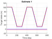
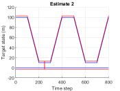
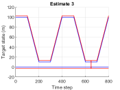
Figure 3: Scenario of the example. We have a ground truth set of trajectories with two trajectories (blue), and four estimated sets of trajectories (red), each with two trajectories. There is track switching in Estimates 2 and 3.

We use the TM with the Euclidean metric as the base distance and parameters $c=5$, $p=1$, $\gamma=10$, and we normalise its result by the length of the time window $T$. The TW-TM has the same parameters as the TM with the normalised weights for online trackers in (17) with $\rho=0.995$. The OSPA⁽²⁾ metric also uses the Euclidean metric, $c=5$, $p=1$ and is applied on the same time interval. We have also tested the trajectory metrics with $\gamma=10^{8}$ to show the results when assignments are not allowed to change in time, as in OSPA⁽²⁾.

The resulting errors and the decomposition into (time-weighted) localisation cost for properly detected targets (Loc.), cost for missed targets (Mis.), cost for false targets (Fal.) and cost for track switches (Swi.) are shown in Table I, and the resulting rankings in Table II. The TW-TM ranks the algorithms according to what we would expect for an online tracker. The TM ranks the algorithm well, but indicates that E2 and E3 have the same error, as for this metric, it does not matter when the track switches take place. The error decomposition provides relevant information about the estimates. On the contrary, OSPA⁽²⁾ does not rank the algorithms properly; E4 is ranked as the second best algorithm despite the major errors in the estimation of one trajectory. This type of localisation error is typically penalised more than a track switch in most MOT applications [6, Sec. 13.6]. Setting $\gamma=\infty$ or $\gamma$ sufficiently high in the trajectory metrics also has undesirable effects in the ranking, due to the lack of change in the assignments [6].

Table I: Errors and their decomposition for the estimates in Figure 3

Metric	TW-TM					TM					OSPA(2)	TW-TM ($\gamma=10^{8}$)	TM ($\gamma=10^{8}$)
	Tot.	Loc.	Mis.	Fal.	Swi.	Tot.	Loc.	Mis.	Fal.	Swi.	Tot.	Tot.	Tot.
$\mathrm{E}1$	6	6	0	0	0	6	6	0	0	0	3	6	6
$\mathrm{E}2$	6.01	6.00	0	0	0.01	6.03	6.00	0	0	0.03	3.62	6.18	7.25
$\mathrm{E3}$	6.05	6.00	0	0	0.05	6.03	6.00	0	0	0.03	3.38	7.84	6.76
$\mathrm{E}4$	7.46	3.81	1.82	1.82	0	6.63	5.06	0.78	0.78	0	3.31	7.46	6.63

Table II: Ranking of the estimates for the different metrics

Metric	Ranking
TW-TM	E1-E2-E3-E4
TM	E1-E2-E3-E4
	E1-E3-E2-E4
OSPA(2)	E1-E4-E3-E2
TW-TM ($\gamma=10^{8}$)	E1-E2-E4-E3
TM ($\gamma=10^{8}$)	E1-E4-E3-E2

Finally, we show the decomposition of the error across time, see Section IV-B, for the TW-TM and the TM in Figure 4. This decomposition provides useful information, for example, we can locate when track switching occurs, and determine that there are not any missed or false targets.

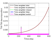
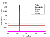
Figure 4: Decomposition of the error across time for the time-weighted trajectory metric (left) and the trajectory metric (right) for Estimate 2 in Figure 3. In the TW-TM, the (time-weighted) costs increase with time due to the considered weighting, see (17).

VII Conclusions

This paper has extended the metric on sets of trajectories in [1] to include weights to penalise the costs (localisation error, number of missed/false targets, and track switches) at different time steps unevenly. This extension adds flexibility to the trajectory metric [1] to suit more user preferences to compute the error of multiple object tracking algorithms.

The metric can be computed solving a multi-dimensional assignment problem, e.g., using the Viterbi algorithm. The LP relaxation of the metric is also a metric and is computable in polynomial time.

Appendix A

In this appendix, we prove Proposition 3. The non-negativity, identity and symmetry properties of the metric in (14) are straightforward. The proof of the triangle inequality is analogous to the proof of the triangle inequality of the trajectory metric [1, App. B], with some minor adaptations.

The proof in this section is done for the LP metric, where the optimization is over $W^{k}\in\mathcal{\overline{W}}_{\mathbf{X},\mathbf{Y}}$. The proof is similar for the multi-dimensional assignment metric in (5), where the optimisation is over $W^{k}\in\mathcal{W}_{\mathbf{X},\mathbf{Y}}$. We use $\overline{d}\left(\mathbf{X},\mathbf{Y},W^{1:T}\right)$ to denote the objective function in (14) as a function of $W^{1:T}=\left(W^{1},...,W^{T}\right)$.

The outline of the triangle inequality proof is as follows. We assume that we have three sets of trajectories $\mathbf{X}$, $\mathbf{Y}$, $\mathbf{Z}$. Let $W_{\mathbf{X},\mathbf{Z}}^{\star,k}$ and $W_{\mathbf{Z},\mathbf{Y}}^{\star,k}$ be the weight matrices that minimise $\overline{d}\left(\mathbf{Y},\mathbf{Z},W^{1:T}\right)$ and $\overline{d}\left(\mathbf{Z},\mathbf{Y},W^{1:T}\right)$. Based on $W_{\mathbf{X},\mathbf{Z}}^{\star,k}$ and $W_{\mathbf{Z},\mathbf{Y}}^{\star,k}$, we construct a matrix $W_{\mathbf{X},\mathbf{Y}}^{k}\in\mathcal{\overline{W}}_{\mathbf{X},\mathbf{Y}}$ such that

$$W_{\mathbf{X},\mathbf{Y}}^{k}(i,j) =\sum_{l=1}^{n_{\mathbf{Z}}}W_{\mathbf{X},\mathbf{Z}}^{\star,k}(i,l)W_{\mathbf{Z},\mathbf{Y}}^{\star,k}(l,j)$$ (25)

for $i\in\{1,...,n_{\mathbf{X}}\}$ and $j\in\{1,...,n_{\mathbf{Y}}\}$, and the rest of the elements of $W_{\mathbf{X},\mathbf{Y}}^{k}$ are

$$W_{\mathbf{X},\mathbf{Y}}^{k}(i,j)$$

$$=\begin{cases}1-\sum_{j=1}^{n_{\mathbf{Y}}}W_{\mathbf{X},\mathbf{Y}}^{k}(i,j)&i\in\{1,...,n_{\mathbf{X}}\},j=n_{\mathbf{Y}}+1\\ 1-\sum_{i=1}^{n_{\mathbf{X}}}W_{\mathbf{X},\mathbf{Y}}^{k}(i,j)&i=n_{\mathbf{X}}+1,j\in\{1,...,n_{\mathbf{Y}}\}\\ 0&i=n_{\mathbf{X}}+1,j=n_{\mathbf{Y}}+1.\end{cases}$$ (26)

Then, we show that

$$\overline{d}\left(\mathbf{X},\mathbf{Y},W_{\mathbf{X},\mathbf{Y}}^{1:T}\right) \leq\overline{d}\left(\mathbf{X},\mathbf{Z}\right)+\overline{d}\left(\mathbf{Z},\mathbf{Y}\right).$$ (27)

By definition, $\overline{d}\left(\mathbf{X},\mathbf{Y}\right)\leq\overline{d}\left(\mathbf{X},\mathbf{Y},W_{\mathbf{X},\mathbf{Y}}^{1:T}\right)$, which yields

$$\overline{d}\left(\mathbf{X},\mathbf{Y}\right) \leq\overline{d}\left(\mathbf{X},\mathbf{Z}\right)+\overline{d}\left(\mathbf{Z},\mathbf{Y}\right)$$ (28)

and finishes the proof of the triangle inequality.

To prove (27), we show that for any $W_{\mathbf{X},\mathbf{Z}}^{k}\in\mathcal{\overline{W}}_{\mathbf{X},\mathbf{Z}}$ and $W_{\mathbf{Z},\mathbf{Y}}^{k}\in\mathcal{\overline{W}}_{\mathbf{Z},\mathbf{Y}}$, and $W_{\mathbf{X},\mathbf{Y}}^{k}$ obtained using (25) and (26). we have

$$\overline{d}\left(\mathbf{X},\mathbf{Y},W_{\mathbf{X},\mathbf{Y}}^{1:T}\right) \leq\overline{d}\left(\mathbf{X},\mathbf{Z},W_{\mathbf{X},\mathbf{Z}}^{1:T}\right)+\overline{d}\left(\mathbf{Z},\mathbf{Y},W_{\mathbf{Z},\mathbf{Y}}^{1:T}\right).$$ (29)

We prove (29) in Section A-B. Before this, we provide three preliminary inequalities in Section A-A.

A-A Preliminary inequalities

The following switching cost inequality holds [1, App. B]

$$\sum_{i=1}^{n_{\mathbf{X}}}\sum_{j=1}^{n_{\mathbf{Y}}}\left|W_{\mathbf{X},\mathbf{Y}}^{k}\left(i,j\right)-W_{\mathbf{X},\mathbf{Y}}^{k+1}\left(i,j\right)\right|$$

$$\leq\sum_{i=1}^{n_{\mathbf{X}}}\sum_{l=1}^{n_{\mathbf{Z}}}\left|W_{\mathbf{X},\mathbf{Z}}^{k}\left(i,l\right)-W_{\mathbf{X},\mathbf{Z}}^{k+1}\left(i,l\right)\right|$$

$$\quad+\sum_{j=1}^{n_{\mathbf{Y}}}\sum_{l=1}^{n_{\mathbf{Z}}}\left|W_{\mathbf{Z},\mathbf{Y}}^{k}\left(l,j\right)-W_{\mathbf{Z},\mathbf{Y}}^{k+1}\left(l,j\right)\right|.$$ (30)

The following inequality also holds [1, App. B],

$$\mathrm{tr}\big{[}\big{(}D_{\mathbf{X},\mathbf{Y}}^{k}\big{)}^{\dagger}W_{\mathbf{X},\mathbf{Y}}^{k}\big{]}$$

$$\leq\sum_{i=1}^{n_{\mathbf{X}}}\sum_{j=1}^{n_{\mathbf{Y}}}\sum_{l=1}^{n_{\mathbf{Z}}}\left(d_{\mathbf{X},\mathbf{Z}}^{k}\left(i,l\right)+d_{\mathbf{Z},\mathbf{Y}}^{k}\left(l,j\right)\right)^{p}W_{\mathbf{X},\mathbf{Z}}^{k}\left(i,l\right)W_{\mathbf{Z},\mathbf{Y}}^{k}\left(l,j\right)$$

$$\quad+\sum_{j=1}^{n_{\mathbf{Y}}}D_{\mathbf{Z},\mathbf{Y}}^{k}\left(n_{\mathbf{Z}}+1,j\right)W_{\mathbf{Z},\mathbf{Y}}^{k}\left(n_{\mathbf{Z}}+1,j\right)$$

$$\quad+\sum_{j=1}^{n_{\mathbf{Y}}}\sum_{l=1}^{n_{\mathbf{Z}}}\left(d_{\mathbf{X},\mathbf{Z}}^{k}\left(n_{\mathbf{X}}+1,l\right)+d_{\mathbf{Z},\mathbf{Y}}^{k}\left(l,j\right)\right)^{p}$$

$$\quad\times W_{\mathbf{X},\mathbf{Z}}^{k}\left(n_{\mathbf{X}}+1,l\right)W_{\mathbf{Z},\mathbf{Y}}^{k}\left(l,j\right)$$

$$\quad+\sum_{i=1}^{n_{\mathbf{X}}}D_{\mathbf{X},\mathbf{Z}}^{k}\left(i,n_{\mathbf{Z}}+1\right)W_{\mathbf{X},\mathbf{Z}}^{k}\left(i,n_{\mathbf{Z}}+1\right)$$

$$\quad+\sum_{i=1}^{n_{\mathbf{X}}}\sum_{l=1}^{n_{\mathbf{Z}}}\left(d_{\mathbf{X},\mathbf{Z}}^{k}\left(i,l\right)+d_{\mathbf{Z},\mathbf{Y}}^{k}\left(l,n_{\mathbf{Y}}+1\right)\right)^{p}$$

$$\quad\times W_{\mathbf{X},\mathbf{Z}}^{k}\left(i,l\right)W_{\mathbf{Z},\mathbf{Y}}^{k}\left(l,n_{\mathbf{Y}}+1\right)$$ (31)

where $d_{\mathbf{X},\mathbf{Y}}^{k}\left(i,j\right)=D_{\mathbf{X},\mathbf{Y}}^{k}(i,j)^{1/p}$.

Finally, for $p\geq 1$, and $a_{m},b_{m}\geq 0$, the Minkowski inequality [28, pp. 165] is

$$\left(\sum_{m}\left[a_{m}+b_{m}\right]^{p}\right)^{1/p} \leq\left(\sum_{m}a_{m}^{p}\right)^{1/p}+\left(\sum_{m}b_{m}^{p}\right)^{1/p}.$$ (32)

A-B Proof of (29)

From (31), we can write

$$w_{1}^{k}\mathrm{tr}\big{[}\big{(}D_{\mathbf{X},\mathbf{Y}}^{k}\big{)}^{\dagger}W_{\mathbf{X},\mathbf{Y}}^{k}\big{]}$$

$$\leq\sum_{i=1}^{n_{\mathbf{X}}}\sum_{j=1}^{n_{\mathbf{Y}}}\sum_{l=1}^{n_{\mathbf{Z}}}\left(a_{i,l,j}^{k}+b_{i,l,j}^{k}\right)^{p}+\sum_{j=1}^{n_{\mathbf{Y}}}\left(0+b_{j}^{k}\right)^{p}$$

$$+\sum_{j=1}^{n_{\mathbf{Y}}}\sum_{l=1}^{n_{\mathbf{Z}}}\left(a_{l,j}^{k}+b_{l,j}^{k}\right)^{p}+\sum_{i=1}^{n_{\mathbf{X}}}\left(a_{i}^{k}+0\right)^{p}$$

$$+\sum_{i=1}^{n_{\mathbf{X}}}\sum_{l=1}^{n_{\mathbf{Z}}}\left(a_{i,l}^{k}+b_{i,l}^{k}\right)^{p}$$ (33)

where we have multiplied the cost by $w_{1}^{k}$ and it is direct to identify the terms $a_{i,l,j}^{k}$ and $b_{i,l,j}^{k}$ once $w_{1}^{k}$ and the weight matrices are included inside the parenthesis for each summation in (31).

Combining (30) and (31) with $\overline{d}\left(\mathbf{X},\mathbf{Y},W_{\mathbf{X},\mathbf{Y}}^{1:T}\right)$, we obtain

$$\overline{d}\left(\mathbf{X},\mathbf{Y},W_{\mathbf{X},\mathbf{Y}}^{1:T}\right)$$

$$\leq\left[\sum_{k=1}^{T}\left(\sum_{i=1}^{n_{\mathbf{X}}}\sum_{j=1}^{n_{\mathbf{Y}}}\sum_{l=1}^{n_{\mathbf{Z}}}\left(a_{i,l,j}^{k}+b_{i,l,j}^{k}\right)^{p}+\sum_{j=1}^{n_{\mathbf{Y}}}\left(0+b_{j}^{k}\right)^{p}\right.\right.$$

$$+\sum_{j=1}^{n_{\mathbf{Y}}}\sum_{l=1}^{n_{\mathbf{Z}}}\left(a_{l,j}^{k}+b_{l,j}^{k}\right)^{p}+\sum_{i=1}^{n_{\mathbf{X}}}\left(a_{i}^{k}+0\right)^{p}$$

$$\left.+\sum_{i=1}^{n_{\mathbf{X}}}\sum_{l=1}^{n_{\mathbf{Z}}}\left(a_{i,l}^{k}+b_{i,l}^{k}\right)^{p}\right)$$

$$\quad+\sum_{k=1}^{T-1}\sum_{i=1}^{n_{\mathbf{X}}}\sum_{l=1}^{n_{\mathbf{Z}}}\underbrace{\frac{\gamma^{p}}{2}w_{2}^{k}\left|W_{\mathbf{X},\mathbf{Z}}^{k}\left(i,l\right)-W_{\mathbf{X},\mathbf{Z}}^{k+1}\left(i,l\right)\right|}_{\left(a_{i,l}^{k,2}+0\right)^{p}}$$

$$\left.\quad+\sum_{k=1}^{T-1}\sum_{j=1}^{n_{\mathbf{Y}}}\sum_{l=1}^{n_{\mathbf{Z}}}\underbrace{\frac{\gamma^{p}}{2}w_{2}^{k}\left|W_{\mathbf{Z},\mathbf{Y}}^{k}\left(l,j\right)-W_{\mathbf{Z},\mathbf{Y}}^{k+1}\left(l,j\right)\right|}_{\left(0+b_{l,j}^{k,2}\right)^{p}}\right]^{1/p}.$$ (34)

We make use of the Minkowski inequality (32) to obtain

$$\overline{d}\left(\mathbf{X},\mathbf{Y},W_{\mathbf{X},\mathbf{Y}}^{1:T}\right)$$

$$\leq\left[\sum_{k=1}^{T}\left(\sum_{i=1}^{n_{\mathbf{X}}}\sum_{j=1}^{n_{\mathbf{Y}}}\sum_{l=1}^{n_{\mathbf{Z}}}\left(a_{i,l,j}^{k}\right)^{p}+\sum_{j=1}^{n_{\mathbf{Y}}}\sum_{l=1}^{n_{\mathbf{Z}}}\left(a_{l,j}^{k}\right)^{p}\right.\right.$$

$$\left.+\sum_{i=1}^{n_{\mathbf{X}}}\left(a_{i}^{k}+0\right)^{p}+\sum_{i=1}^{n_{\mathbf{X}}}\sum_{l=1}^{n_{\mathbf{Z}}}\left(a_{i,l}^{k}\right)^{p}\right)$$

$$\left.+\sum_{k=1}^{T-1}\sum_{i=1}^{n_{\mathbf{X}}}\sum_{l=1}^{n_{\mathbf{Z}}}\frac{\gamma^{p}}{2}w_{2}^{k}\left|W_{\mathbf{X},\mathbf{Z}}^{k}\left(i,l\right)-W_{\mathbf{X},\mathbf{Z}}^{k+1}\left(i,l\right)\right|\right]^{1/p}$$

$$+\left[\sum_{k=1}^{T}\left(\sum_{i=1}^{n_{\mathbf{X}}}\sum_{j=1}^{n_{\mathbf{Y}}}\sum_{l=1}^{n_{\mathbf{Z}}}\left(b_{i,l,j}^{k}\right)^{p}+\sum_{j=1}^{n_{\mathbf{Y}}}\left(0+b_{j}^{k}\right)^{p}\right.\right.$$

$$\left.+\sum_{j=1}^{n_{\mathbf{Y}}}\sum_{l=1}^{n_{\mathbf{Z}}}\left(b_{l,j}^{k}\right)^{p}+\left.\sum_{i=1}^{n_{\mathbf{X}}}\sum_{l=1}^{n_{\mathbf{Z}}}\left(b_{i,l}^{k}\right)^{p}\right)\right)$$

$$\left.+\sum_{k=1}^{T-1}\sum_{j=1}^{n_{\mathbf{Y}}}\sum_{l=1}^{n_{\mathbf{Z}}}\frac{\gamma^{p}}{2}w_{2}^{k}\left|W_{\mathbf{Z},\mathbf{Y}}^{k}\left(l,j\right)-W_{\mathbf{Z},\mathbf{Y}}^{k+1}\left(l,j\right)\right|\right]^{1/p}.$$ (35)

By using (31) and (33), we proceed to write the terms that include a coefficient $a_{i,l,j}^{k}$ in terms of the distances. We have

$$\sum_{i=1}^{n_{\mathbf{X}}}\sum_{j=1}^{n_{\mathbf{Y}}}\sum_{l=1}^{n_{\mathbf{Z}}}\left(a_{i,l,j}^{k}\right)^{p}+\sum_{j=1}^{n_{\mathbf{Y}}}\sum_{l=1}^{n_{\mathbf{Z}}}\left(a_{l,j}^{k}\right)^{p}$$

$$+\sum_{i=1}^{n_{\mathbf{X}}}\left(a_{i}^{k}+0\right)^{p}+\sum_{i=1}^{n_{\mathbf{X}}}\sum_{l=1}^{n_{\mathbf{Z}}}\left(a_{i,l}^{k}\right)^{p}$$

$$=\sum_{i=1}^{n_{\mathbf{X}}}\sum_{j=1}^{n_{\mathbf{Y}}}\sum_{l=1}^{n_{\mathbf{Z}}}w_{1}^{k}d_{\mathbf{X},\mathbf{Z}}^{k}\left(i,l\right)^{p}W_{\mathbf{X},\mathbf{Z}}^{k}\left(i,l\right)W_{\mathbf{Z},\mathbf{Y}}^{k}\left(l,j\right)$$

$$+\sum_{j=1}^{n_{\mathbf{Y}}}\sum_{l=1}^{n_{\mathbf{Z}}}w_{1}^{k}d_{\mathbf{X},\mathbf{Z}}^{k}\left(n_{\mathbf{X}}+1,l\right)^{p}W_{\mathbf{X},\mathbf{Z}}^{k}\left(n_{\mathbf{X}}+1,l\right)W_{\mathbf{Z},\mathbf{Y}}^{k}\left(l,j\right)$$

$$+\sum_{i=1}^{n_{\mathbf{X}}}w_{1}^{k}D_{\mathbf{X},\mathbf{Z}}^{k}\left(i,n_{\mathbf{Z}}+1\right)W_{\mathbf{X},\mathbf{Z}}^{k}\left(i,n_{\mathbf{Z}}+1\right)$$

$$+\sum_{i=1}^{n_{\mathbf{X}}}\sum_{l=1}^{n_{\mathbf{Z}}}w_{1}^{k}d_{\mathbf{X},\mathbf{Z}}^{k}\left(i,l\right)^{p}W_{\mathbf{X},\mathbf{Z}}^{k}\left(i,l\right)W_{\mathbf{Z},\mathbf{Y}}^{k}\left(l,n_{\mathbf{Y}}+1\right)$$

$$=w_{1}^{k}\mathrm{tr}\big{[}\big{(}D_{\mathbf{X},\mathbf{Z}}^{k}\big{)}^{\dagger}W_{\mathbf{X},\mathbf{Z}}^{k}\big{]}$$

where the last equality follows from [1, Eq. (52)]. Similarly, the sums of the terms with coefficient $b_{i,l,j}^{k}$ sum to $w_{1}^{k}\mathrm{tr}\big{[}\big{(}D_{\mathbf{Z},\mathbf{Y}}^{k}\big{)}^{\dagger}W_{\mathbf{Z},\mathbf{Y}}^{k}\big{]}$. Substituting these values into (35) yields (29), which implies that the triangle inequality holds.

References

- [1] A. F. García-Fernández, A. S. Rahmathullah, and L. Svensson, “A metric on the space of finite sets of trajectories for evaluation of multi-target tracking algorithms,” IEEE Transactions on Signal Processing, vol. 68, pp. 3917–3928, 2020.
- [2] R. P. S. Mahler, Advances in Statistical Multisource-Multitarget Information Fusion. Artech House, 2014.
- [3] A. F. García-Fernández, L. Svensson, and M. R. Morelande, “Multiple target tracking based on sets of trajectories,” IEEE Transactions on Aerospace and Electronic Systems, vol. 56, no. 3, pp. 1685–1707, Jun. 2020.
- [4] A. Milan, L. Leal-Taixé, I. Reid, S. Roth, and K. Schindler, “MOT16: a benchmark for multi-object tracking.” [Online]. Available: https://arxiv.org/abs/1603.00831
- [5] T. M. Apostol, Mathematical Analysis. Addison Wesley, 1974.
- [6] S. Blackman and R. Popoli, Design and Analysis of Modern Tracking Systems. Artech House, 1999.
- [7] B. E. Fridling and O. E. Drummond, “Performance evaluation methods for multiple-target-tracking algorithms,” vol. 1481, 1991, pp. 371–383.
- [8] O. E. Drummond and B. E. Fridling, “Ambiguities in evaluating performance of multiple target tracking algorithms,” in Proceedings of the SPIE conference, 1992, pp. 326–337.
- [9] D. Schuhmacher and A. Xia, “A new metric between distributions of point processes,” Advances in Applied Probability, vol. 40, no. 3, pp. 651–672, Sep. 2008.
- [10] D. Schuhmacher, B.-T. Vo, and B.-N. Vo, “A consistent metric for performance evaluation of multi-object filters,” IEEE Transactions on Signal Processing, vol. 56, no. 8, pp. 3447–3457, Aug. 2008.
- [11] A. F. García-Fernández and L. Svensson, “Spooky effect in optimal OSPA estimation and how GOSPA solves it,” in Proceedings on the 22nd International Conference on Information Fusion, 2019.
- [12] A. S. Rahmathullah, A. F. García-Fernández, and L. Svensson, “Generalized optimal sub-pattern assignment metric,” in 20th International Conference on Information Fusion, 2017, pp. 1–8.
- [13] K. Bernardin and R. Stiefelhagen, “Evaluating multiple object tracking performance: The CLEAR MOT metrics,” EURASIP Journal on Image and Video Processing, vol. 2008, pp. 1–10, 2008.
- [14] E. Ristani, F. Solera, R. Zou, R. Cucchiara, and C. Tomasi, “Performance measures and a data set for multi-target, multi-camera tracking,” in ECCV 2016 Workshops, pp. 17–35.
- [15] J. Luiten et al., “HOTA: A higher order metric for evaluating multi-object tracking,” International Journal of Computer Vision, pp. 1–31, 2020.
- [16] B. Ristic, B.-N. Vo, D. Clark, and B.-T. Vo, “A metric for performance evaluation of multi-target tracking algorithms,” IEEE Transactions on Signal Processing, vol. 59, no. 7, pp. 3452–3457, July 2011.
- [17] R. Canavan, C. McCullough, and W. J. Farrell, “Track-centric metrics for track fusion systems,” in 12th International Conference on Information Fusion, 2009, pp. 1147–1154.
- [18] M. Silbert, “A robust method for computing truth-to-track assignments,” in 12th International Conference on Information Fusion, 2009, pp. 1658–1664.
- [19] K. Manson and P. O’Kane, “Taxonomic performance evaluation for multitarget tracking systems,” IEEE Transactions on Aerospace and Electronic Systems, vol. 28, no. 3, pp. 775–787, July 1992.
- [20] M. Beard, B. T. Vo, and B. Vo, “A solution for large-scale multi-object tracking,” IEEE Transactions on Signal Processing, vol. 68, pp. 2754–2769, 2020.
- [21] J. Bento and J. J. Zhu, “A metric for sets of trajectories that is practical and mathematically consistent,” 2018. [Online]. Available: https://arxiv.org/abs/1601.03094
- [22] A. O. Hero III, D. A. Castañón, D. Cochran, and K. Kastella, Foundations and Applications of Sensor Management. Springer, 2008.
- [23] K. Granström, L. Svensson, Y. Xia, J. L. Williams, and A. F. García-Fernández, “Poisson multi-Bernoulli mixture trackers: continuity through random finite sets of trajectories,” in 21st International Conference on Information Fusion, 2018, pp. 973–981.
- [24] K. Granström, L. Svensson, Y. Xia, J. Williams, and A. F. García-Fernández, “Poisson multi-Bernoulli mixtures for sets of trajectories,” 2019. [Online]. Available: https://arxiv.org/abs/1912.08718
- [25] Y. C. Tang and R. Salakhutdinov, “Multiple futures prediction,” in 33rd Conference on Neural Information Processing Systems, 2019.
- [26] A. F. García-Fernández and S. Maskell, “Continuous-discrete trajectory PHD and CPHD filters,” in 23rd International Conference on Information Fusion, 2020, pp. 1–8.
- [27] H. Caesar et al., “nuScenes: A multimodal dataset for autonomous driving,” in IEEE/CVF Conference on Computer Vision and Pattern Recognition (CVPR), 2020, pp. 11 618–11 628.
- [28] C. S. Kubrusly, The Elements of Operator Theory. Springer Science + Business Media, 2011.