A deep learning driven pseudospectral PCE based FFT homogenization algorithm for complex microstructures

Abstract

This work is directed to uncertainty quantification of homogenized effective properties for composite materials with complex, three dimensional microstructure. The uncertainties arise in the material parameters of the single constituents as well as in the fiber volume fraction. They are taken into account by multivariate random variables. Uncertainty quantification is achieved by an efficient surrogate model based on pseudospectral polynomial chaos expansion and artificial neural networks. An artificial neural network is trained on synthetic binary voxelized unit cells of composite materials with uncertain three dimensional microstructures, uncertain linear elastic material parameters and different loading directions. The prediction goals of the artificial neural network are the corresponding effective components of the elasticity tensor, where the labels for training are generated via a fast Fourier transform based numerical homogenization method. The trained artificial neural network is then used as a deterministic solver for a pseudospectral polynomial chaos expansion based surrogate model to achieve the corresponding statistics of the effective properties. Three numerical examples deal with the comparison of the presented method to the literature as well as the application to different microstructures. It is shown, that the proposed method is able to predict central moments of interest while being magnitudes faster to evaluate than traditional approaches.

Algorithm [label1] organization= Chair of Engineering Mechanics, University of Paderborn, addressline=Warburger Str. 100, city=Paderborn, postcode=33098, country=Germany

A deep learning algorithm for homogenization of uncertain complex microstructures is proposed

A neural network is trained on three dimensional microstructures discretized by voxels and homogenized with FFT

The geometry of the microstructures considered as well as their corresponding material parameters are modeled as random variables

Uncertainty quantification is carried out by pseudospectral polynomial chaos expansion, utilizing the trained neural network as efficient solver

Several numerical examples compare the performance of the proposed method with respect to standard methods such as FEM and Monte Carlo

1 Introduction

Composite materials consist of multiple constituents on the micro scale. This leads to a heterogeneous microstructure in the sense of geometry as well as material behavior. In this work, composites with two constituents of linear elastic material are discussed. One constituent acts as a matrix, whereas the second is embedded in the former as inclusions. The geometry of the inclusions can either be long fibers, short fibers or particles [1]. The microstructure and the material behavior of its constituents determine the overall effective material behavior of the composite on the macro scale. To obtain the effective macro properties, homogenization techniques like analytical mean-field [2] or numerical full-field approaches are used, where the later takes the microstructure into account explicitly. For complex microstructures such as short fiber inclusions, analytical mean-field methods perform poorly [3]. Full-field approaches on the other hand can deal with arbitrary microstructures [3].

Microstructures as well as the material properties of the composite and underlying constituents are subjected to uncertainties, grounded in either intrinsic variety or induced by the manufacturing or measuring methods [4, 5]. This is especially true for short fiber reinforced materials, where not only the microstructures and inclusion geometries are very complex, but also the measurement and imaging is challenging and dependent on many factors [6]. Uncertainties on the micro scale lead to uncertain effective properties of the composite at the macro scale, which requires uncertainty quantification (UQ).

This works follows the framework of [7], where UQ consists of three steps. First, the sources of uncertainties (e.g. microstructures and material parameters) need to be quantified, e.g. by defining distributions of random variables based on measurements and expert knowledge. Second, an appropriate computational model of the problem studied needs to be defined. At last, the uncertainties are propagated through the model to achieve the distribution of the output, the so called quantity of interest (QoI). Universal techniques for this purpose are Monte Carlo-type methods (MC) including simple Monte Carlo and Latin Hyper-cube sampling [8]. Although they can be used on existing computational models by simply sampling from the input distribution and repeatedly running it, they suffer from low efficiency due to slow convergence [9].

To address this problem, so called surrogate models can be used instead [7]. These apply some kind of dimension reduction e.g. on the input parameters. Examples are polynomial chaos expansion (PCE, [10, 11]), low-rank tensor representations [12], support-vector machines and radial basis functions.

Uncertainties in the context of continuum micromechanics were studied extensively in e.g. [13]. Here, a generic meso-scale probability model for a large class of random anisotropic elastic microstructures in the context of tensor-valued random fields is proposed, which is not limited to a specific microstructure defined by its constituents. The stochastic boundary value problem is solved using the stochastic finite element method (FEM). In [14], a dualistic deterministic / stochastic method is considered, utilizing two models coupled in an Arlequin framework. A framework using bounded random matrices for constitutive modeling is proposed in [15], which results in a surrogate, which can be calibrated to experimental data. In [16], a new class of generalized nonparametric probabilistic models for matrix-valued non-Gaussian random fields is investigated, where the focus is on random field taking values in some subset of the set of real symmetric positive-definite matrices presenting sparsity and invariance with respect to given orthogonal transformations. An approach using stochastic potential in combination with a polynomial chaos representation for nonlinear constitutive equations of materials in the context of random microstrucutral geometry and high dimensional random parameters is given in [17]. PCE was further used in homogenization by [18] and [19]. The later proposed an intrusive PCE in combination with FEM based full-field homogenization [20] to determine uncertain effective material properties of transversely linear elastic fiber reinforced composites. The intrusive approach to PCE uses Galerkin projection, where the FEM algorithm needs to be reformulated using PC arithmetic [21].

While in [19] cylindrical single fiber inclusions are homogenized, in this work the uncertain homogenization method is adjusted to more complex microstructures. For this it is convenient to replace the FEM homogenization scheme by a fast Fourier transform (FFT) [22] based on the FFT Galerkin approach by [23, 24]. This method uses voxels and is more efficient in terms of CPU time and memory requirement than FEM, as shown in [25] and [26]. To adapt PCE to FFT, the Galerkin projection is replaced by the pseudospectral PCE [27] to avoid PC arithmetics. Pseudospectral PCE uses numerical integration techniques to obtain the PC coefficients. From this surrogate model, the central moments of the QoI can be calculated. The pseudospectral approach is called a non-intrusive method, as only repeated deterministic solutions from the solver are needed instead of using PC arithmetic. Here, the computational bottleneck is the deterministic solver [28].

To reduce the computational effort of the deterministic solution, data driven machine learning models trained on the deterministic solver can be used to replace the original model [29]. Popular approaches are decision trees, random forest ensembles, radial basis functions and support vector machines. While relatively easy to train, they are limited to either linear approximations or suffer from excessive parameters, especially in the case of large three dimensional image data [30]. An alternative approach is the use of artificial neural networks (ANN). ANN, especially in the context of deep learning, gained much attention, mainly because of its impact in fields like computer vision, speech recognition and autonomous driving [29]. The universal approximation theorem [31] states, that ANN can learn any Borel measurable function if the network has enough units. Additionally, there exist special architectures to effectively handle large image data. There are already several applications of ANN to computational continuum mechanics. For an overview the reader should refer to [29]. ANN were successfully used as surrogate models in the context of MC based uncertainty quantification of elliptic differential equations [32] and MC application on three dimensional homogenization [33]. While there were some applications to homogenization, these were limited to either two dimensional microstructures [34], uniaxial strain [35] or fixed material parameters [36, 37].

To the authors knowledge there was no attempt to apply ANN to homogenization of multiple three dimensional microstructures with uncertain material parameters and different loading directions. This work intends to close this gap by establishing a complete homogenization technique based on ANN. Due to the fast evaluation time of trained ANN, this homogenization technique is very efficient, as shown in this work. The ANN can then be used to carry out otherwise expensive stochastic investigations like pseudospectral PCE, where multiple deterministic solutions are necessary. In summary the key objectives and contributions of this work are:

• Deep Learning homogenization algorithm: An ANN is trained to homogenize uncertain three dimensional complex microstructures with uncertain material parameters subjected to different loading directions.

• FFT Label Generation: FFT is used to provide the labels needed for training of the ANN. This is done on voxel based three dimensional microstructures without meshing

• UQ with pseudospectral PCE: A pseudospectral PCE using an ANN trained on FFT is used for UQ of the uncertain effective elasticity tensor of complex microstructures

The rest of the paper is structured as follows. In Section 2 the theoretical base of pseudospectral PCE, FFT based homogenization and ANN is given. Section 3 is concerned with the proposed homogenization model of using ANN in UQ in the context of pseudospectral PCE. Here the general problem formulation, data creation, network topology and training of the ANN as well as the UQ using pseudospectral PCE are discussed. Section 4 consists of three numerical experiments. One aims to compare the proposed method with [19], whereas the second is dedicated to a more complex microstructure, showing also the computational efficiency of the ANN accelerated approach to UQ. The third example investigates the abillity of the ANN to generalize to unseen microstructures. The paper closes with a summary and an outlook in Section 5.

2 Preliminaries

This section gives essential prerequisites of random variables, uncertainty quantification, deep learning and numerical homogenization, which are used in the proposed algorithm in Section 3.

2.1 Random variables and uncertainty quantification

Let $(\Omega,\Sigma,P)$ be a probability space [38] with sample space $\Omega$, $\sigma$-algebra $\Sigma$, and a probability measure $P$ on $\Omega$. A multivariate random input variable $\mathbf{X}$ is defined by the map

$$\mathbf{X}:\left\{\begin{aligned} &\Omega&\to&\quad\mathcal{D}_{\mathbf{X}}\subset\mathbb{R}^{n_{x}}\\ &\omega&\mapsto&\quad\mathbf{X}(\omega)=\mathbf{x},\end{aligned}\right.$$ ((1))

where $\mathcal{D}_{\mathbf{X}}\subset\mathbb{R}^{n_{x}}$ is an $n_{x}$ dimensional vector-space of realizations $\mathbf{x}$ of elementary events $\omega\in\Omega$ by the map $\mathbf{X}$. A model $\mathcal{M}$ then takes multivariate random input variables $\mathbf{X}(\omega)$ and maps them to multivariate random variables $\mathbf{Y}(\omega)$ defined by the relation

$$\mathcal{M}:\left\{\begin{aligned} &\mathcal{D}_{\mathbf{X}}&\to&\quad\mathcal{D}_{\mathbf{Y}}\subset\mathbb{R}^{n_{y}}\\ &\mathbf{X}(\omega)&\mapsto&\quad\mathcal{M}(\mathbf{X}(\omega))=\mathbf{Y}(\omega)=\mathbf{y},\end{aligned}\right.$$ ((2))

where $\mathcal{D}_{\mathbf{Y}}\subset\mathbb{R}^{n_{y}}$ is an $n_{y}$ dimensional vector-space of realizations $\mathbf{y}$ of elementary events $\omega\in\Omega$ by the composition function $\mathbf{Y}=\mathcal{M}\circ\mathbf{X}:\Omega\to\mathcal{D}_{\mathbf{Y}}$. The goal of uncertainty quantification (UQ) is to characterize the distribution of the output vector $\mathbf{Y}(\omega)$ for a given input vector $\mathbf{X}(\omega)$ in Eq. (1), thus propagating input uncertainties through the model $\mathcal{M}$. Often the original model $\mathcal{M}$ is computationally demanding. Therefore, surrogate models $\tilde{\mathcal{M}}$ can be designed, which approximate the original model but take less computing time to evaluate, as

$$\tilde{\mathcal{M}}:\left\{\begin{aligned} &\mathcal{D}_{\mathbf{X}}&\to&\quad\tilde{\mathcal{D}}_{\mathbf{Y}}\subseteq{\mathcal{D}}_{\mathbf{Y}}\subset\mathbb{R}^{n_{y}}\\ &\mathbf{X}(\omega)&\mapsto&\quad\tilde{\mathcal{M}}(\mathbf{X}(\omega))=\tilde{\mathbf{Y}}(\omega)=\tilde{\mathbf{y}},\end{aligned}\right.$$ ((3))

where $\tilde{\mathcal{D}}_{\mathbf{Y}}\subseteq{\mathcal{D}}_{\mathbf{Y}}\subset\mathbb{R}^{n_{y}}$ is an $n_{y}$ dimensional vector-space of realizations $\tilde{\mathbf{y}}$ of $\omega\in\Omega$ by the composition function $\tilde{\mathbf{Y}}=\tilde{\mathcal{M}}\circ\mathbf{X}:\Omega\to\tilde{\mathcal{D}}_{\mathbf{Y}}$. Due to approximations, the datasets $\tilde{\mathcal{D}}_{\mathbf{Y}}$ and ${\mathcal{D}}_{\mathbf{Y}}$ usually do not coincide. This means, that two mappings of the same realization $\mathbf{X}(\omega)=\mathbf{x}$ by the original model $\mathcal{M}$ in Eq. (2) and a surrogate model $\tilde{\mathcal{M}}$ are not the same. The distance between $\mathcal{M}$ and $\tilde{\mathcal{M}}$ defines an error function [39]

$$\mathcal{E}=||\mathcal{M}(\mathbf{X}(\omega))-\tilde{\mathcal{M}}(\mathbf{X}(\omega))||_{2}=\sqrt{\mathbb{E}[\mathcal{M}(\mathbf{X}(\omega))-\tilde{\mathcal{M}}(\mathbf{X}(\omega))]^{2}},$$ ((4))

with expectation $\mathbb{E}$ defined component wise as the integral

$${\displaystyle\mathbb{E}[\mathbf{X}(\omega)]=\operatorname{E}[(X_{1}(\omega),\ldots,X_{n_{x}}(\omega))]=(\mathbb{E}[X_{1}(\omega)],\ldots,\mathbb{E}[X_{n_{x}}(\omega)])},\qquad\displaystyle\mathbb{E}[X(\omega)]=\int_{\Omega}X(\omega)\,\mathrm{d}{P},$$ ((5))

over a probability space $(\Omega,\Sigma,P)$. For a surrogate model $\tilde{\mathcal{M}}$ to have a small error $\mathcal{E}$ with respect to the original model $\mathcal{M}$ in Eq. (2), it must be calibrated on a dataset $\mathbb{D}$, which consists of evaluations of an original model $\mathcal{M}$ with regard to a finite number $n_{s}$ of realizations $\mathbf{x}_{k}\subset\mathcal{D}_{\mathbf{X}}$, called samples, of $\mathbf{X}(\omega)$ in Eq. (1), such that

$$\mathbb{D}=\left\{(\mathbf{x}_{k},\mathbf{y}_{k}),\;k=1,\dots,n_{s}\right\}.$$ ((6))

2.2 Surrogate modelling by PCE

An example of a surrogate model as described in Eq. (3) is provided by a Polynomial Chaos Expansion $\tilde{\mathcal{M}}_{PCE}$ defined as

$$1.\quad\tilde{\mathcal{M}}_{PCE}(\mathbf{X}(\omega))=\tilde{\mathbf{Y}}(\omega)=\displaystyle\sum_{|\mathbf{i}|\leq n_{PCE}}\hat{\mathbf{Y}}_{\mathbf{i}}\Psi_{\mathbf{i}}(\mathbf{\theta}(\omega)),\qquad\text{where}$$

$$2.\quad\hat{\mathbf{Y}}_{\mathbf{i}}=\displaystyle\frac{1}{\gamma_{\mathbf{i}}}\mathbb{E}\left[\tilde{\mathbf{Y}}(\omega)\Psi_{\mathbf{i}}(\mathbf{\theta}(\omega))\right]=\displaystyle\frac{1}{\gamma_{\mathbf{i}}}\left\langle\tilde{\mathbf{Y}}(\omega),\Psi_{\mathbf{i}}(\mathbf{\theta}(\omega))\right\rangle=\displaystyle\frac{1}{\gamma_{\mathbf{i}}}\displaystyle\int\tilde{\mathbf{Y}}(\omega)\Psi_{\mathbf{i}}(\mathbf{\theta}(\omega))\mathrm{d}F_{\tilde{\mathbf{Y}}}$$

$$3.\quad\gamma_{\mathbf{i}}=\mathbb{E}\left[\Psi_{\mathbf{i}}^{2}\right]=\left\langle\Psi_{\mathbf{i}},\Psi_{\mathbf{i}}\right\rangle$$

$$4.\quad F_{\tilde{\mathbf{Y}}}(\tilde{\mathbf{y}})=P\left(\tilde{\mathbf{Y}}_{1}(\omega)\leq\tilde{\mathbf{y}}_{1},\ldots,\tilde{\mathbf{Y}}_{n_{y}}(\omega)\leq\tilde{\mathbf{y}}_{n_{y}}\right)$$ ((7))

Here, $\Psi_{\mathbf{i}}(\mathbf{\theta}(\omega))$ are orthonormal polynomials, which act as basis functions of the expansion with truncation order $n_{PCE}$, $\gamma_{\mathbf{i}}$ are normalization factors with inner product $\left\langle\bullet,\bullet\right\rangle$, $\mathbf{\theta}(\omega)$ denote standard normal distributed random variables and $F_{\tilde{\mathbf{Y}}}$ is the cumulative distribution function (CDF) with respect to the multivariate random variable $\tilde{\mathbf{Y}}(\omega)$. In Eq. (7) and throughout the remaining sections of this paper, $\mathbf{i}$ is a multi-index over the random input space $\mathcal{D}_{\mathbf{X}}\subset\mathbb{R}^{n_{x}}$ in Eq. (1)

$$\mathbf{i}=(i_{1},\dots,i_{n_{x}})\in\mathbb{N}_{0}^{n_{x}},\quad|\mathbf{i}|=i_{1}+{\dots}+i_{n_{x}}.$$ ((8))

The calibration of $\tilde{\mathcal{M}}_{PCE}$ from Eq. (7) to the original model $\mathcal{M}$ in Eq. (2) is performed by calculating the PC coefficients $\hat{\mathbf{Y}}_{\mathbf{i}}$ in Eq. (7.2). To this end, the so called pseudospectral approach to PCE uses a cubature rule for selection of the samples in the dataset in Eq. (6), where the number of samples $n_{s}$ equals the number of cubature nodes $\Theta$, i.e. $n_{s}=n_{q}$, such that

$$\mathbb{D}_{cub}=\left\{(\mathbf{x}_{k}=\Theta_{k},\dots,\mathbf{x}_{n_{q}}=\Theta_{n_{q}}),(\mathcal{M}(\Theta_{k}),\dots,\mathcal{M}(\Theta_{n_{q}})),\;k=1,\dots,n_{s}=n_{q}\right\}.$$ ((9))

Here $\Theta_{k},\;k=1,\dots,{\color[rgb]{0,0,0}n_{q},}$ denotes the single index form of the cubature nodes. Accordingly with $\tilde{\mathbf{Y}}(\omega)$ the PC coefficients in Eq. (7.2) are approximated as

$$\hat{\mathbf{Y}}_{\mathbf{i}}\approx\displaystyle\frac{1}{\gamma_{\mathbf{i}}}\displaystyle\sum_{j=1}^{n_{w}}{\mathcal{M}}(\Theta^{(j)})\Psi_{\mathbf{i}}(\Theta^{(j)})w(\Theta^{(j)}),$$ ((10))

where $\Theta^{(j)},j=1,\dots,n_{w}$, represents the multi-index form of a cubature rule with dimension $n_{x}$ and weights $w(\Theta^{(j)})$, where $n_{w}$ denotes the number of nodes and weights per dimension $n_{x}$. The total number of cubature points $\mathbf{x}_{n_{q}}$ needed in Eq. (9) is

$$n_{q}=(n_{w})^{n_{x}},$$ ((11))

as the cubature rule with $n_{w}$ nodes $\Theta^{(j)}$ and corresponding weights $w(\Theta^{(j)})$ must be carried out over all dimensions $n_{x}$ of the input random vector space $\mathcal{D}_{\mathbf{X}}\subset\mathbb{R}^{n_{x}}$ in Eq. (1). The relation in Eq. (11) holds true for equal number of nodes and weights $n_{w}$ per dimension $n_{x}$, as it is the case in the reminder of this work. Generally, $n_{w}$ can be chosen differently for each dimension.

In this paper, the central moments of interest of the input $\mathbf{X}(\omega)$ and output $\mathbf{Y}(\omega)$ are the mean

$$\boldsymbol{\mu}_{\mathbf{X}}=\mathbb{E}\left[\mathbf{X}(\omega)\right],\quad\boldsymbol{\mu}_{\mathbf{X}}\in{\color[rgb]{0,0,0}\mathbb{R}^{n_{x}}}$$ ((12))

with expectation defined in Eq. (5) and variance with standard deviation $\boldsymbol{\sigma}_{\mathbf{X}}$

$$\boldsymbol{\sigma}_{\mathbf{X}}^{2}=\text{var}(\mathbf{X}(\omega))=\mathbb{E}\left[(\mathbf{X}(\omega)-\mathbb{E}\left[(\mathbf{X}(\omega)\right])^{2}\right],\quad\boldsymbol{\sigma}\in{\color[rgb]{0,0,0}\mathbb{R}^{n_{x}}_{+}}.$$ ((13))

The mean $\boldsymbol{\mu}_{\mathbf{Y}}$ and the standard deviation $\boldsymbol{\sigma}_{\mathbf{Y}}$ can be calculated from the PC coefficients $\hat{\mathbf{Y}}_{\mathbf{i}}$ in Eq. (10) by the following relations

$$\boldsymbol{\mu}_{\mathbf{Y}}=\mathbb{E}\left[\mathcal{M}(\mathbf{X}(\omega))\right]\approx\mathbb{E}\left[\tilde{\mathcal{M}}(\mathbf{X}(\omega))\right]\approx\hat{\mathbf{Y}}_{\mathbf{0}}\in{\color[rgb]{0,0,0}\mathbb{R}^{n_{y}}}$$ ((14))

$$\boldsymbol{\sigma}_{\mathbf{Y}}^{2}=\text{var}({\hat{\mathbf{Y}}}_{\mathbf{i}})=\mathbb{E}\left[({\mathcal{M}(\mathbf{X}(\omega)})-\boldsymbol{\mu})^{2}\right]\approx\displaystyle\sum_{0<|\mathbf{i}|\leq n_{PCE}}\left[\gamma_{\mathbf{i}}\hat{\mathbf{Y}}_{\mathbf{i}}^{2}\right]\in{\color[rgb]{0,0,0}\mathbb{R}^{n_{y}}_{+}}.$$ ((15))

For a more detailed treatment, the reader is referred to [38, 39, 40].

2.3 Surrogate modeling by ANN

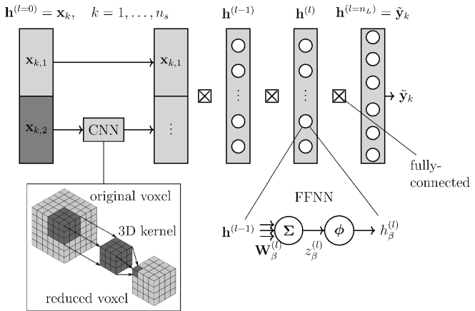
Figure 1: Schematic structure of an ANN in Eq. (16) with $n_{L}$ layers $\mathbf{h}^{(l)}$ and $n_{u}$ neural units $h_{\beta}^{(l)}$. An ANN with input ${\mathbf{x}}_{k}=\{{\mathbf{x}}_{k,1},{\mathbf{x}}_{k,2}\}$, where ${\mathbf{x}}_{k,1}$ is a numerical vector and ${\mathbf{x}}_{k,2}$ consist of 3D voxel data. ${\mathbf{x}}_{k,2}$ is first processed by a CNN in Eq. (19) and after concatenation with ${\mathbf{x}}_{k,1}$ feed into an FFNN in Eq. (17). The resulting output is $\mathbf{h}^{(n_{L})}=\tilde{{\mathbf{y}}}_{k}$. The index $k=1,\dots,n_{s}$, denotes the single samples, where $n_{s}$ is the number of samples.

Deep learning using ANN is a subbranch of machine learning, which is a subbranch of artificial intelligence [41, 30]. An ANN, as visualized in Figure 1, is a surrogate model $\tilde{\mathcal{M}}_{ANN}$ in Eq. (3), which is built of $n_{L}$ layers $\mathbf{h}^{(l)}$ consisting of $n_{u}$ neural units $h_{\beta}^{(l)}$

$$\mathbf{h}^{(0)}=\mathbf{x}_{k},\quad\mathbf{h}^{(l)}=\left\{h_{\beta}^{(l)},\beta=1,\dots,n_{u}\right\},\quad\mathbf{h}^{(L)}=\tilde{{\mathbf{y}}}_{k},\quad l=0,\dots,n_{L}.$$ ((16))

Here, $\mathbf{h}^{(0)}$ is the first layer consisting of input samples ${\mathbf{x}}_{k}$ from a dataset $\mathbb{D}$ according to Eq. (6), where $k=1,\dots,n_{s}$, denotes single samples of $\mathbb{D}$ and $n_{s}$ the number of samples. Furthermore, $\mathbf{h}^{(n_{L})}$ is the last layer consisting of predictions $\tilde{\mathbf{y}}_{k}=\tilde{\mathcal{M}}_{ANN}(\tilde{\mathbf{x}}_{k})$ with respect to the input ${\mathbf{x}}_{k}$. For the neural units $h_{\beta}^{(l)}$ in Eq. (16), several architectures exist, where the following are used throughout this paper:

• Densely connected Feed Forward Neural Network (FFNN)

  $$h_{\beta}^{(l)}=\phi\left(\mathbf{W}_{\beta}^{(l)}\mathbf{h}^{(l-1)}\right)=\phi({z}_{\beta}^{(l)}),$$ ((17))

  where $\mathbf{W}_{\beta}^{(l)}$ are weights for every unit $h_{\beta}^{(l)}$, which are multiplied with the output of the preceding layer $\mathbf{h}^{(l-1)}$. These weights are stored in a matrix $\mathbf{W}=\left\{\mathbf{W}_{\beta}^{(l)}\right\}$ for the whole network. After multiplication of weights $\mathbf{W}_{\beta}^{(l)}$ and output $\mathbf{h}^{(l-1)}$, a nonlinear activation function $\phi$ is applied to the product in Eq. (17). This is important for the network to be able to represent non-linearities. In this paper, rectified linear units (ReLU) [42]) are used

  $$\phi(z_{\beta}^{(l)})=\text{max}\left\{0,z_{\beta}^{(l)}\right\}.$$ ((18))

• Convolutional Neural Network (CNN) for three dimensional image data utilizing voxels, using a 3D kernel and the convolution operation

  $$h_{\beta}^{(l)}=\{h_{f,xyz}^{(l)}\}=\left\{\phi\left(\displaystyle\sum_{m=1}^{n_{F}^{(l-1)}}\displaystyle\sum_{p=0}^{n_{K}^{(l)}-1}\displaystyle\sum_{q=0}^{n_{K}^{(l)}-1}\displaystyle\sum_{r=0}^{n_{K}^{(l)}-1}k_{fm,pqr}^{(l)}h_{m,(x+p)(y+q)(z+r)}^{(l-1)}\right)\right\},$$ ((19))

  where $\{h_{f,xyz}^{(l)}\}$ denotes the output voxel of filter $f$, with $n_{F}$ being the number of filters, which are equivalent to the number of neural units $n_{u}$ of FFNN. $k_{fm,pqr}^{(l)}$ is the three dimensional kernel, which, similar to Eq. (17), can be gathered in a matrix $\mathbf{K}=\{k_{fm,pqr}^{(l)}\}$ for the whole network and $n_{K}$ is the kernel dimension.

The so called topology of an ANN is then the composition of neural units $h_{\beta}^{(l)}$ in Eq. (16) with their corresponding architectures FFNN in Eq. (17) and CNN in Eq. (19) to a network [43]. The calibration of the surrogate in Eq. (16), also called training, consists of comparing the output data ${\mathbf{y}}_{k}$ of a model $\mathcal{M}$, defined in Eq. (2), from a dataset $\mathbb{D}$ in Eq. (6) consisting of predictions $\tilde{{\mathbf{y}}}_{k}(\mathbf{W},\mathbf{K})$ from an ANN $\tilde{\mathcal{M}}_{ANN}$ in Eq. (16) with weights $\mathbf{W}$ in Eq. (17) or kernels $\mathbf{K}$ in Eq. (19). Consequently, the error function $\mathcal{E}$ in Eq. (4) takes the form

$$\mathcal{E}=\displaystyle\sum_{k}^{n_{s}}||\mathbf{y}_{k}-\tilde{\mathbf{y}}_{k}(\mathbf{W},\mathbf{K})||_{2}=\displaystyle\sum_{k}^{n_{s}}\sqrt{\mathbb{E}[\mathbf{y}_{k}-\tilde{\mathbf{y}}_{k}(\mathbf{W},\mathbf{K})]^{2}},$$ ((20))

where $k$ and $n_{s}$ are defined means of Eq. (6). This leads to a minimization problem, where an L2-regularization term $\mathcal{R}(\mathbf{W},\mathbf{K})$ is added

$$\operatorname*{arg\,min}_{\mathbf{W},\mathbf{K}}\;\left\{\mathcal{E}+\mathcal{R}(\mathbf{W},\mathbf{K})\right\}=\operatorname*{arg\,min}_{\mathbf{W},\mathbf{K}}\;\left\{||\mathbf{y}_{k}-\tilde{\mathbf{y}}_{k}(\mathbf{W},\mathbf{K})||_{2}+\underbrace{\lambda_{L2}||\mathbf{W},\mathbf{K}||_{2}^{2}}_{\text{$\mathcal{R}(\mathbf{W},\mathbf{K})$}}\right\},$$ ((21))

with regularization factor $\lambda_{L2}$. The regularization term $\mathcal{R}(\mathbf{W},\mathbf{K})$ in Eq. (21) is added to prevent overfitting, where the exact value for the regularization factor $\lambda_{L2}$ needs to be thoroughly tuned. Typically, $\lambda_{L2}\approx 0.01$ is used [44]. The weights $\mathbf{W}$ or kernels $\mathbf{K}$ are then updated iteratively by gradient descent of the error function $\mathcal{E}$ in Eq. (20) with respect to the weights or kernels, respectively

$$\mathbf{W}\leftarrow\mathbf{W}-\alpha\frac{\partial\mathcal{E}}{\partial\mathbf{W}},\quad\mathbf{K}\leftarrow\mathbf{K}-\alpha\frac{\partial\mathcal{E}}{\partial\mathbf{K}},$$ ((22))

where $\alpha$ denotes the gradient descent step width, also called learning rate. For further details the reader is referred to standard works such as [45, 41, 30].

2.4 Numerical homogenization

The following section gives an overview of numerical homogenization in micromechanics. A comprehensive treatment of the topic can be found in [2, 1, 46].

Following the notation of [47, 24, 48, 22], a microstructure is represented as a unit cell

$$\mathbb{M}(\zeta_{i},\omega)=(0,\xi_{1})\otimes(0,\xi_{2})\otimes(0,\xi_{3}),\qquad\zeta_{i}=0,\dots,\xi_{i},\qquad i=1,2,3,$$ ((23))

with properties

$$\mathbb{M}(\zeta_{i},\omega)=\begin{cases}1\quad\text{if}\quad\zeta_{i}\in\mathbb{M}^{I}(\omega)\\ 0\quad\text{if}\quad\zeta_{i}\in\mathbb{M}^{M}(\omega),\end{cases}$$ ((24))

where $\xi_{i}$ are dimensions and $\zeta_{i}$ are coordinates inside the unit cell $\mathbb{M}(\zeta_{i},\omega)$, which consists of a matrix phase $\mathbb{M}^{M}(\omega)$ and inclusion phases $\mathbb{M}^{I}(\omega),\quad\mathbb{M}(\zeta_{i},\omega)=\mathbb{M}^{M}(\omega)\cup\mathbb{M}^{I}(\omega)$. The uncertain indicator function in Eq. (24) identifies the different phases at different coordinates $\zeta_{i}$ (see e.g. [17]). In this work the outer dimensions $\xi_{i}$ of the unit cell $\mathbb{M}(\zeta_{i},\omega):=\mathbb{M}(\omega)$ are deterministic and constant. An uncertain micro elasticity problem is defined as

$$1.\quad\nabla\cdot\boldsymbol{\sigma}(\omega)=\mathbf{0}$$

$$2.\quad\boldsymbol{\sigma}(\omega)=\mathbb{C}(\omega):\boldsymbol{\varepsilon}(\omega)$$

$$3.\quad\boldsymbol{\varepsilon}(\omega)=\frac{1}{2}(\nabla\otimes\mathbf{u}(\omega)+(\nabla\otimes\mathbf{u}(\omega))^{T})$$

$$4.\quad\bar{b}(\omega)\quad\text{on}\quad\partial\mathbb{M},$$ ((25))

where $\boldsymbol{\sigma}(\omega)$ is an uncertain micro stress tensor, $\mathbb{C}(\omega)$ an uncertain micro elasticity tensor, $\boldsymbol{\varepsilon}(\omega)$ an uncertain micro strain tensor and $\mathbf{u}(\omega)$ an uncertain micro displacement tensor. Here, Eq. (25.1) denotes equilibrium conditions, Eq. (25.2) and Hooke’s law, Eq. (25.3) strain-displacement conditions. For the boundary value problem in Eq. (25) to be well posed, uncertain boundary conditions $\bar{b}(\omega)$ are introduced in Eq. (25.4), where $\partial\mathbb{M}$ denotes the boundary of the corresponding unit cell $\mathbb{M}(\omega)$ in Eq. (23). Possible choices are Dirichlet, Neumann or periodic boundary conditions.

Accounting also for periodicity, the uncertain micro strain tensor $\boldsymbol{\varepsilon}(\omega)$ in Eq. (25.3) can be split into an average deterministic macro strain tensor $\bar{\boldsymbol{\varepsilon}}$ and an $\mathbb{M}$-periodic fluctuating uncertain micro strain tensor $\boldsymbol{\varepsilon}^{*}(\omega)$

$$\boldsymbol{\varepsilon}(\omega)=\bar{\boldsymbol{\varepsilon}}+\boldsymbol{\varepsilon}^{*}(\omega),\qquad\displaystyle\int_{\mathbb{M}}\boldsymbol{\varepsilon}^{*}(\omega)\mathrm{d}\boldsymbol{\zeta}=\boldsymbol{0},$$ ((26))

where the fluctuating part $\boldsymbol{\varepsilon}^{*}(\omega)$ must be compatible (continuous and single-valued) to an $\mathbb{M}$-periodic displacement field. The uncertain micro elasticity tensor $\mathbb{C}(\omega)$ in Eq.(25.2) depends on uncertain material parameters $\boldsymbol{\kappa}(\omega)$ of phases $(i)$ in Eq. (24), such that

$${\color[rgb]{0,0,0}\mathbb{C}(\boldsymbol{\kappa}^{(i)}(\omega))=K^{(i)}(\omega)\mathbf{1}\otimes\mathbf{1}+2G^{(i)}(\omega)\mathbb{I}^{\text{dev}},\quad i=M,I,}$$ ((27))

with

$${\color[rgb]{0,0,0}\boldsymbol{\kappa}(\omega)=\{\kappa_{1}^{(i)}(\omega),\kappa_{2}^{(i)}(\omega)\}\equiv\{\lambda^{(i)}(\omega),G^{(i)}(\omega)\}\equiv\{\text{E}^{(i)}(\omega),\nu^{(i)}(\omega)\}\equiv\{\text{K}^{(i)}(\omega),{\color[rgb]{0,0,0}G^{(i)}(\omega)}\},}$$ ((28))

where $\lambda^{(i)}(\omega)$ is the uncertain first Lamé constant, $G^{(i)}(\omega)$ the uncertain shear modulus, $E^{(i)}(\omega)$ the uncertain Young’s modulus, $\nu^{(i)}(\omega)$ the uncertain Poisson’s ratio and $K^{(i)}(\omega)$ the uncertain bulk modulus. Solving the uncertain boundary value problem in Eq. (25) on an uncertain microstructure $\mathbb{M}(\omega)$ in Eq. (23) and using an average operator on the micro fields, one obtains corresponding effective macro fields

$$\bar{\boldsymbol{\varepsilon}}=\langle\boldsymbol{\varepsilon}(\omega)\rangle,\quad\bar{\boldsymbol{\sigma}}(\omega)=\langle\boldsymbol{\sigma}(\omega)\rangle,\quad{\color[rgb]{0,0,0}\bar{\boldsymbol{\sigma}}(\omega)=\bar{\mathbb{C}}(\omega):\bar{\boldsymbol{\varepsilon}}(\omega)}$$ ((29))

where $\bar{\boldsymbol{\sigma}}(\omega)$ denotes an uncertain effective macro stress tensor, $\bar{\boldsymbol{\varepsilon}}$ a deterministic effective macro strain tensor and $\bar{\mathbb{C}}(\omega)$ an uncertain effective macro elasticity tensor. The average operator $\langle\bullet\rangle$ in Eq. (29) is defined as

$$\langle\bullet\rangle=\displaystyle\frac{1}{\mathbb{M}}\displaystyle\int_{\mathbb{M}}(\bullet)\mathrm{d}\mathbb{M}.$$ ((30))

The macro and micro stress and strain fields need to satisfy the Hill-Mandel condition:

$$\langle\boldsymbol{\sigma}(\omega):\boldsymbol{\varepsilon}(\omega)\rangle=\langle\boldsymbol{\sigma}(\omega)\rangle:\langle\boldsymbol{\varepsilon}(\omega)\rangle.$$ ((31))

Numerical homogenization can be represented by a model $\mathcal{M}$ in Eq. (2) with random input variable in $\mathbf{X}(\omega)$ Eq. (1) and random output variable $\mathbf{Y}(\omega)$ in Eq. (2) defined as

$$1.\quad\mathbf{X}(\omega)=\{\boldsymbol{\kappa}(\omega),\mathbb{M}(\omega),\bar{b}(\omega)\},$$

$${\color[rgb]{0,0,0}2.\quad\mathbf{Y}(\omega)=\bar{\mathbb{C}}(\omega)=\mathcal{M}(\boldsymbol{\kappa}(\omega),\mathbb{M}(\omega),\bar{b}(\omega)).}$$ ((32))

The model $\mathcal{M}$ in Eq. (32) can be realized e.g. by an FFT-based homogenization method $\mathcal{M}=\mathcal{M}_{FFT}$, based on [47, 24, 48]. Following [48], a brief overview of the FFT-based homogenization scheme is sketched. For detailed explanations, the reader is referred to the above mentioned papers. As a point of departure, the uncertain micro elasticity problem is recast into the weak form using test strains $\delta\boldsymbol{\varepsilon^{*}}$, such that

$$\int_{\mathbb{M}}\delta\varepsilon^{*}:\boldsymbol{\sigma}(\boldsymbol{\zeta},\bar{\boldsymbol{\varepsilon}}+\boldsymbol{\varepsilon}^{*}(\omega))\mathrm{d}\boldsymbol{\zeta}=\displaystyle\int_{\mathbb{M}}\left[\mathbb{G}\star\delta\varepsilon^{*}\right]:\boldsymbol{\sigma}(\boldsymbol{\zeta},\bar{\boldsymbol{\varepsilon}}+\boldsymbol{\varepsilon}^{*}(\omega))\mathrm{d}\boldsymbol{\zeta}=0,$$ ((33))

where the compatibility of the test strains is enforced by means of a convolution $\star$ with a projection operator to compatible solutions $\mathbb{G}$. This projection operator also enforces the zero-mean condition in Eq. (26) and is known analytically in Fourier space. Carrying out discretization by means of trigonometric polynomials and solving integrals by quadrature rules, the following expression in matrix notation holds

$$\underline{\underline{\mathbb{G}}}:\underline{\underline{\sigma}}(\underline{\underline{\varepsilon}}(\omega))=\underline{0}.$$ ((34))

The model $\mathcal{M}_{\text{FFT}}$ is then established by solving for the unknown micro strain field $\boldsymbol{\varepsilon}(\omega)$ in Eq. (34) using strain boundary conditions and projection based iterative methods such as e.g. the conjugate gradient method. After solving Eq. (34), the uncertain effective macro elasticity tensor can be recovered from Eq. (29). By prescribing the uncertain macro strain tensor $\bar{b}(\omega)=\bar{\boldsymbol{\varepsilon}}(\omega)$ from Eq. (25), Eq. (32.2) then becomes

$$\bar{\mathbb{C}}(\omega)\approx\mathcal{M}_{{FFT}}(\boldsymbol{\kappa}(\omega),\mathbb{M}(\omega),\bar{\boldsymbol{\varepsilon}}(\omega))=:\bar{\mathbb{C}}_{FFT}(\omega).$$ ((35))

Remarks:

1. Attempts in the literature to use ANN in microstructural homogenization were either restricted to two dimensions, uniaxial strain or fixed material parameters, using FEM instead of FFT. A short overview is given in Table 1.

2. For uncertain homogenization calculating the full elasticity tensor ${\mathbb{C}}(\omega)$ in Eq. (27), three dimensional microstructures $\mathbb{M}(\omega)$ in Eq. (23), multiaxial strain $\mathbf{\varepsilon}(\omega)$ in Eq. (29) and varying material parameters $\mathbf{\kappa}(\omega)$ in Eq. (28) are needed.

3. For complex microstructures, where meshing for FEM becomes expensive, FFT as in Eq. (34) is a mesh free alternative.

4. It has to be carefully distinguished between an untrained ANN and a trained ANN. The trained ANN is deterministic, as it’s weights are fixed after optimization. For the rest of the paper, the untrained ANN will be denoted by $\tilde{\mathcal{M}}_{ANN}$ and the trained ANN by $\tilde{\mathcal{M}}_{ANN}^{t}$.

5. There are several choices for boundary conditions to solve the boundary value problem in Eq. (25). In this work, the FFT-based Galerkin method of [47, 24, 48] is used, which works directly with strains instead of displacements and enforces compatibility of the solution by a projection operator to compatible solutions. Therefore, strain boundary conditions are used.

6. The following sections propose an algorithm to take these points into account, namely by considering three dimensional, uncertain microstructures with uncertain material parameters and multiple loading directions.

Author	Microstructures	Material parameters	Loading	Uncertainty
[34]	three dimensional	fixed	one direction	fully deterministic
[37]	two dimensional	fixed	one direction	fully deterministic
[35]	two dimensional	fixed	one direction	fully deterministic
[33]	three dimensional	fixed	multiple directions	uncertain microstructure
Present	three dimensional	variable	multiple directions	fully uncertain

Table 1: Overview of similar homogenization methods using ANN from selected authors.

3 A deep learning uncertain FFT algorithm

In a previous work, [19] investigate an uncertain numerical homogenization method of long fiber reinforced plastics. Uncertainties of material parameters and geometry are considered and modeled by multivariate random variables. The homogenization is carried out by the finite element method (FEM) utilizing periodic boundary conditions over a meshed representative volume element. To propagate the input uncertainties and calculate effective uncertain properties after homogenization, an intrusive Galerkin projection PCE is used. In this work, an extension towards more complex microstructures is made. In the following, the framework of the proposed method is presented, followed by detailed explanations of the implementation.

3.1 Uncertain homogenization framework

It was shown in e.g. [25] and [26], that FFT based homogenization schemes outperform FEM based full field homogenization techniques with respect to CPU time and memory requirement. FFT based homogenization methods, as described in Eq. (34), are meshless. The discretization of the geometry is carried out on a regular grid utilizing voxels. Homogenization using FFT is described by the model $\mathcal{M}_{FFT}$ in Eq. (35), which is used for the evaluation in Eq. (32). The goal is to calculate the uncertain effective macro elasticity tensor $\bar{\mathbb{C}}(\omega)$ in Eq. (29). To calculate central moments like mean in Eq. (14) and variance in Eq. (15) of components of the uncertain effective macro elasticity tensor $\bar{\mathbb{C}}(\omega)$ in Eq. (29), UQ is needed. In this work, a PCE according to Eq. (7) as a surrogate model $\tilde{\mathcal{M}}_{PCE}$ following Eq. (3) is used to approximate Eq. (35)

$$\bar{\mathbb{C}}_{FFT}(\omega)\approx\tilde{\mathcal{M}}_{PCE}(\boldsymbol{\kappa}(\omega),\mathbb{M}(\omega),\bar{\boldsymbol{\varepsilon}})=\displaystyle\sum_{|\mathbf{i}|\leq n_{PCE}}\hat{\mathbb{C}}_{\mathbf{i}}\Psi_{\mathbf{i}}(\mathbf{\theta}(\omega))=:\bar{\mathbb{C}}_{PCE}(\omega),$$ ((36))

where $\mathbf{i}$ is the multi-index in Eq. (8). In order to avoid PC arithmetic like in [19], which is needed for the intrusive Galerkin PCE, the pseudospectral approach in Eq. (10) may be used to approximate the PC coefficients $\hat{\mathbb{C}}_{\mathbf{i}}$ in Eq. (36)

$$\hat{\mathbb{C}}_{\mathbf{i}}\approx\hat{\mathbb{C}}_{\mathbf{i}}^{FFT}=\frac{1}{\gamma_{\mathbf{i}}}\displaystyle\sum_{j=1}^{n_{w}}{\mathcal{M}_{{FFT}}}(\Theta^{(j)})\Psi_{\mathbf{i}}(\Theta^{(j)})w(\Theta^{(j)}),\quad j=1,\dots,n_{w}.$$ ((37))

Here, $\Theta^{(j)}$ and $w(\Theta^{(j)})$ are the nodes and weights of the cubature rule in Eq. (9), which can be gathered in the dataset $\mathbb{D}_{cub}=\mathbb{D}_{FFT}$ from Eq. (9) in single index notation. To this end, $n_{q}$ deterministic solutions of the computational model $\mathcal{M}_{{FFT}}$, as defined in Eq. (11), are needed in Eq. (37)

$$\mathbb{D}_{FFT}=\left\{(\mathbf{x}_{k}=\Theta_{k},\dots,\mathbf{x}_{n_{q}}=\Theta_{n_{q}}),(\mathcal{M}_{FFT}(\Theta_{k}),\dots,\mathcal{M}_{FFT}(\Theta_{n_{q}})),\quad k=1,\dots,n_{q}\right\}.$$ ((38))

In Eq. (38), $\mathbf{x}_{k}=\{\boldsymbol{\kappa}(\omega),\mathbb{M}(\omega),\bar{\boldsymbol{\varepsilon}}\}$ are multivariate realizations of the random input variable $\mathbf{X}(\omega)$ in Eq. (32). Finally the pseudospectral PCE follows from Eq. (36) and Eq. (37) as

$$\bar{\mathbb{C}}_{PCE}(\omega)\approx\displaystyle\sum_{|\mathbf{i}|\leq n_{PCE}}{\hat{\mathbb{C}}^{FFT}_{\mathbf{i}}}\Psi_{\mathbf{i}}(\mathbf{\theta}(\omega)).$$ ((39))

For large unit cells $\mathbb{M}(\omega)$ in Eq. (23), the solution of the problem formulated in Eq. (39) becomes computational challenging due to the large number of evaluations $n_{q}$ of the deterministic model $\mathcal{M}_{FFT}$, which are needed for the PCE as described in Eq. (11). Instead, an ANN $\tilde{\mathcal{M}}_{ANN}$ as defined in Eq. (16) can be trained to learn the deterministic model $\mathcal{M}_{FFT}$, which is faster to evaluate than the original model, because only simple matrix multiplications in FFNN Eq. (17) and CNN Eq. (19) are needed. This approximation can be formulated as

$$\mathcal{M}_{\text{FFT}}\approx\tilde{\mathcal{M}}_{{ANN}}^{t}.$$ ((40))

Eq. (37) is replaced by

$$\hat{\mathbb{C}}_{\mathbf{i}}\approx\hat{\mathbb{C}}^{ANN}_{\mathbf{i}}=\frac{1}{\gamma_{\mathbf{i}}}\displaystyle\sum_{j=1}^{n_{w}}\tilde{\mathcal{M}}_{{ANN}}^{t}(\Theta^{(j)})\Psi_{\mathbf{i}}(\Theta^{(j)})w(\Theta^{(j)}).$$ ((41))

For the approximation Eq. (40) to hold, an ANN $\tilde{\mathcal{M}}_{ANN}$ needs to be trained on a dataset $\mathbb{D}=\mathbb{D}_{ANN}$ in Eq. (6) defined as

$$\mathbb{D}_{ANN}=\left\{(\mathbf{x}_{k}=\left\{\boldsymbol{\kappa}_{k},\boldsymbol{\mathbb{M}}_{k},\boldsymbol{\bar{\varepsilon}}_{k}\right\}),(\mathbf{y}_{k}=\boldsymbol{\bar{\sigma}}=\mathcal{M}_{FFT}(\mathbf{{x}}_{k}),\quad k=1,\dots,n_{s}\right\},$$ ((42))

where $\mathbf{x}_{k}$ need to sample the physically admissible support from $\mathbf{X}(\omega)$ in Eq. (32). Finally Eq. (39) is approximated as

$$\bar{\mathbb{C}}_{PCE}(\omega)\approx\displaystyle\sum_{|\mathbf{i}|\leq{\color[rgb]{0,0,0}n_{PCE}}}{\hat{\mathbb{C}}^{ANN}_{\mathbf{i}}}\Psi_{\mathbf{i}}(\mathbf{\theta}(\omega))=:{\bar{\mathbb{C}}}_{ANN}(\omega).$$ ((43))

This is the final formulation for the proposed UQ FFT model using an ANN $\tilde{\mathcal{M}}_{ANN}$. Once trained, $\tilde{\mathcal{M}}_{ANN}^{t}$ provides the deterministic solutions for the macro elasticity tensor ${\bar{\mathbb{C}}}_{ANN}$ in Eq. (43). From the surrogate $\tilde{\mathcal{M}}_{PCE}$ in Eq. (43), central moments, mean $\boldsymbol{\mu}$ Eq. (14) and variance $\boldsymbol{\sigma}^{2}$ Eq. (15), can be calculated. In the following section, details of the implementation of Eq. (43) are provided.

3.2 Numerical implementation

3.2.1 Algorithm overview

To realize Eq. (43), Algorithm 0 must be implemented. Its task is to generate a training set $\mathbb{D}_{ANN}$ Eq. (42) for training an ANN $\tilde{\mathcal{M}}_{{ANN}}$ to learn FFT homogenization Eq. (35), which is then used for uncertainty quantification of a homogenized elasticity tensor ${\bar{\mathbb{C}}}_{ANN}$ in Eq. (43).

Remark 1: It has to be pointed out, that the ANN $\tilde{\mathcal{M}}_{{ANN}}^{t}$ is a purely deterministic surrogate to the deterministic FFT solver from Eq. (34). After training, the weights of the ANN in Eq. (17) and Eq. (19) are fixed, thus producing deterministic outputs for given deterministic inputs.

The single steps, namely data generation in Section 3.2.2, ANN training in Section 3.2.3 and UQ in Section 3.2.4, are further described in detail.

Algorithm 0 Overall procedure for UQ with PCE and ANN

  Algorithm 1: Data Generation for Deep Learning using FFT

     Input: $\mathbf{X}^{U}(\omega)=\{\boldsymbol{\kappa}^{U}(\omega),\mathbb{M}^{U}(\omega),\bar{\boldsymbol{\varepsilon}}\}\sim\boldsymbol{\mathcal{U}}(\underline{x},\bar{x})$ in Eq. (44)

    Homogenization: $\mathbf{{y}}_{k}=\boldsymbol{\bar{\sigma}}=\mathcal{M}_{FFT}(\mathbf{{x}}_{k})$ in Eq. (47)

    Output: training dataset $\boldsymbol{\mathbb{D}}_{ANN}=\left\{(\mathbf{{x}}_{k}),(\mathbf{{y}}_{k}),\;k=1,\dots,n_{s}\right\},\;\displaystyle\frac{n_{s}}{6}\in\mathbb{N}^{+}$ in Eq. (42)

    

  Algorithm 2: ANN Design and Training

    Input: ${\color[rgb]{0,0,0}\boldsymbol{\mathbb{D}}_{ANN},\tilde{\mathcal{M}}_{ANN}^{t}}$ in Eq. (42) and Eq. (16)

    Training: $\underset{\mathbf{W},\mathbf{K}}{\arg\min}\{\left\|\mathbf{y}_{k}-\tilde{\mathbf{y}}_{k}(\mathbf{W},\mathbf{K})\right\|_{2}+\underbrace{\lambda_{L2}\|\mathbf{W},\mathbf{K}\|_{2}^{2}}_{\mathcal{R}(\mathbf{W},\mathbf{K})}\}$ in Eq. (21)

    Output: $\mathbf{W},\mathbf{K},\tilde{\mathcal{M}}_{{ANN}}^{t}$ in Eq. (40)

  

  Algorithm 3: UQ using PCE and ANN trained on FFT

    Input: $\tilde{\mathcal{M}}_{ANN}^{t},\mathbf{X}(\omega)=\{\boldsymbol{\kappa}(\omega),\mathbb{M}(\omega),\hat{\boldsymbol{\varepsilon}}\}\sim\boldsymbol{\mathcal{N}}(\boldsymbol{\mu},\mathbf{\Sigma})$ in Eq. (40) and Eq. (32)

    Output: ${\color[rgb]{0,0,0}{\bar{\mathbb{C}}}_{ANN}=\tilde{\mathcal{M}}_{\text{PCE}}(\tilde{\mathcal{M}}_{{ANN}}^{t}(\boldsymbol{\kappa}(\omega),\boldsymbol{\mathbb{M}}(\omega),\boldsymbol{\bar{\varepsilon}}_{k}))}$ in Eq. (43)

3.2.2 Data generation for deep learning using FFT

In step 1 of Algorithm ‣ 3.2.1, a dataset $\mathbb{D}_{ANN}$ from Eq. (42) is created with Algorithm 1. The inputs to the dataset $\mathbb{D}_{ANN}$ are realizations $\mathbf{{x}}_{k}$ of an input random variable denoted by $\mathbf{X}^{U}(\omega)$ from Eq. (1), such that

$$\mathbf{X}^{U}(\omega)=\mathbf{{x}}_{k}=\left\{\boldsymbol{\kappa}_{k},\boldsymbol{\mathbb{M}}_{k},\boldsymbol{\bar{\varepsilon}}_{k}\right\}\in\mathcal{D}_{\boldsymbol{X}}^{U},\quad k=1,\dots,n_{s},$$ ((44))

where $\mathbb{M}_{k}$ are microstructures as described in Eq. (23), $\boldsymbol{\kappa}_{k}$ are material parameters defined in Eq. (28), $\bar{\boldsymbol{\varepsilon}}_{k}$ are macro strains from Eq. (29) and $\mathcal{D}_{\boldsymbol{X}}^{U}$ denotes the sample space of the training input variables. The total number of samples of the dataset $\mathbb{D}_{ANN}$ is denoted by $n_{s}$, consistent with Eq. (6).

Generally, the only influence on the outcome of the ANN $\tilde{\mathcal{M}}_{ANN}^{t}$ in Eq. (40) is the training process including the data provided during training. The choice of inputs in Eq. (44) for the training dataset $\mathbb{D}_{ANN}$ from Eq. (42) is therefore very important. Clustering around specific values of e.g. the fiber volume fraction $c_{f,k}$ or the material parameters $\kappa_{k}$ in the dataset could lead to a bias towards these values. Having in mind the goal to establish a deterministic surrogate to replace the FFT solver from Eq. (34), the inputs from Eq. (44) to the dataset $\mathbb{D}_{ANN}$ should fill their sample space ${\mathcal{D}}_{\boldsymbol{X}}^{U}$ from Eq. (44) uniformly. Therefore, the inputs $x_{k}$ from Eq. (44) are drawn from uniform distributions $\boldsymbol{X}^{U}(\omega)\sim\boldsymbol{\mathcal{U}}(\underline{x},\bar{x})$. Additionally, physically inadmissible values must be avoided. Therefore, the sample space ${\mathcal{D}}_{\boldsymbol{X}}^{U}$ from Eq. (44) needs to be restricted. In implementation practise, these values are drawn from uniform distributions, whereas the lower and upper bounds $\underline{x}$ and $\bar{x}$, respectively, have to be chosen in accordance with physical restrictions. Therefore the general expression of ${\mathcal{D}}_{\boldsymbol{X}}\subset\mathbb{R}$ is specified from Eq. (1) to Eq. (44) as

$$\mathcal{D}_{\boldsymbol{X}}^{U}=\begin{cases}\mathcal{D}_{\boldsymbol{X}}^{{\kappa}_{i}}=\{{\kappa}_{i}:[\underline{\kappa}_{i}\leq{\kappa}_{i}\leq\bar{\kappa}_{i}]\},\;i=1,\ldots,n_{p}\\ \mathcal{D}_{\boldsymbol{X}}^{c_{f}}=\{c_{f}:[0\leq c_{f}\leq 1]\}.\end{cases}$$ ((45))

Here, ${\kappa}_{i}$ denote the single material parameters from Eq. (28). The total number of material parameters is denoted by $n_{p}$. The upper and lower bounds, $\underline{\kappa}_{i}$ and $\bar{\kappa}_{i}$, respectively, are chosen according to the respective admissible range of the material parameter, e.g. $[\underline{\nu}=0\leq\nu\leq\bar{\nu}=0.5]$ for Poisson’s ratio, which is the range for typical engineering materials, including those considered in this work.

The microstructure $\mathbb{M}_{k}$ from Eq. (44) is implemented as a three dimensional voxel array, where the entries are binary, such that $0$ is used for matrix and $1$ for inclusion material. This is mathematically described by the indicator function $\mathbb{M}(\zeta_{i},\omega)$ in Eq. (24). The microstructure $\mathbb{M}$ depends on the fiber volume fraction $c_{f}$ as

$$\mathbb{M}_{k}=\mathbb{M}_{k}(c_{f,k}),$$ ((46))

where $c_{f,k}$ is specific to each microstructure for each $k$ in Eq. (44). In this work, two kinds of microstructures are considered, namely single long fiber cylindrical inclusions and multiple spherical inclusions. The latter are generated by the random sequential adsorption method, as described in [49].

Furthermore, shear and bulk modulus, $G$ and $K$ as described in Eq. (28), respectively, are used as material parameters in the implementation. They are better suited for ANN, because their ranges are of the same magnitude compared to the combination Young’s modulus $E$ and Poisson’s ratio $\nu$ in Eq. (28), which leads to smoother gradient updates in the optimization defined in Eq. (22). Other material parameters are converted internally.

The output $\mathbf{y}_{k}$ for the error measure $\mathcal{E}$ in Eq. (21) is calculated by FFT from Eq. (34). In this work, $\mathbf{y}_{k}$ is the effective macro stress $\mathbf{y}_{k}=\bar{\boldsymbol{{\sigma}}}_{k}$ in Eq. (29) corresponding to the macro strain $\bar{\boldsymbol{\varepsilon}}_{k}$ in Eq. (29) and Eq. (44), such that

$$\mathbf{y}_{k}=\mathcal{M}_{\text{FFT}}({\mathbf{x}}_{k})=\bar{\boldsymbol{{\sigma}}}_{k},\qquad n=1,\dots,n_{s}.$$ ((47))

The effective elasticity tensor $\bar{\mathbb{C}}_{k}$ in Eq. (29) can be reconstructed using Voigt notation such that

$$\bar{{\mathbb{C}}}=\left[\bar{\underline{\underline{\mathbb{C}}}}\right]=[\bar{\underline{{\sigma}}}_{1},\bar{\underline{{\sigma}}}_{2},\bar{\underline{{\sigma}}}_{3},\bar{\underline{{\sigma}}}_{4},\bar{\underline{{\sigma}}}_{5},\bar{\underline{{\sigma}}}_{6}],\qquad\bar{\underline{{\sigma}}}_{i}=\langle\underline{\underline{\mathbb{C}}}\;\underline{\bar{\boldsymbol{\varepsilon}}}_{i}\rangle,\;i=1,\cdots,6.$$ ((48))

$$\underline{\bar{\boldsymbol{\varepsilon}}}_{i}(j)=\begin{cases}1\quad\text{for}\quad i=j,\;j=1,\cdots,6\\ 0\quad\text{else},\end{cases}$$

e.g. for $i=1,\quad\underline{\bar{\boldsymbol{\varepsilon}}}_{i}=1=[1\;0\;0\;0\;0\;0]^{T}.$ The different strain states $\underline{\bar{\boldsymbol{\varepsilon}}}_{i}$ for Eq. (48) need to be equally represented in the dataset Eq. (38). If one strain state would be underrepresented, the predictive capability for that specific state $\underline{\bar{\boldsymbol{\varepsilon}}}_{i}$ would be poor. Therefore, the total number of samples $n_{s}$ must be a multiple of 6, which implies $1/6\;n_{s}\in\mathbb{N}^{+}$ or

$$n_{\boldsymbol{\bar{\underline{\varepsilon}}}_{i}}=n_{\boldsymbol{\bar{\underline{\varepsilon}}}_{j}},\;i,j=1,\cdots,6,$$ ((49))

where $n_{\boldsymbol{\bar{\underline{\varepsilon}}}_{i}}$ denotes the number of samples with strain state $i$. In practise, a compromise between the number of samples $n_{s}$ and the training time has to be made. In the examples in Section 4, $n_{s}=9000$ for Example 1, $n_{s}=13800$ for Example 2 and $n_{s}=9000+13800=22800$ for Example 3. The whole process of data generation can be carried out on a workstation with GPU acceleration or on a cluster, because every sample generation is pleasingly parallel.

Remark 2: An alternative approach to Eq. (48) would be to apply all six strain states directly. This however would lead to less flexibility of the obtained ANN. The proposed approach in Eq. (48) using single strain states $\underline{\bar{\boldsymbol{\varepsilon}}}_{i}$ allows to consider different stochastic properties for different strain states in Algorithm 4. This is the case, if e.g. material parameters are obtained from experimental data, which show different deviations for different loading directions.

Algorithm 1 Data Generation for Deep Learning using FFT

   Input: $\mathbf{X}^{U}(\omega)=\{\boldsymbol{\kappa}^{U}(\omega),\mathbb{M}^{U}(\omega),\bar{\boldsymbol{\varepsilon}}\}\sim\boldsymbol{\mathcal{U}}(\underline{x},\bar{x})$ in Eq. (44)

  Output: ${\mathbb{D}}_{ANN}=\left\{({\mathbf{x}}_{k}),({\mathbf{y}}_{k}),\;k=1,\dots,n_{s}\right\},\;\displaystyle\frac{n_{s}}{6}\in\mathbb{N}^{+}$

  

  $n_{\boldsymbol{\bar{\underline{\varepsilon}}}_{i}}=n_{s}\;/\;6$

  $k=1$

  for $i=1:6$ do

        $\bar{\underline{\boldsymbol{\varepsilon}}}=[0,0,0,0,0,0]$

        $\bar{\underline{\boldsymbol{\varepsilon}}}[i]=1$

        for $q=1:n_{\boldsymbol{\bar{\underline{\varepsilon}}}_{i}}$ do

              Sample $\boldsymbol{\kappa}_{k}\in\mathcal{D}_{\boldsymbol{X}}$

              Sample $c_{f}\in\mathcal{D}_{\boldsymbol{X}}$ and generate $\boldsymbol{\mathbb{M}}_{k}(c_{f})$

              $\boldsymbol{x}_{k}=\{\boldsymbol{\kappa}_{k},\boldsymbol{\mathbb{M}}_{k},\boldsymbol{\bar{\varepsilon}}_{k}\}$

              Solve $\mathbb{G}:\boldsymbol{\sigma}=\mathbf{0}$ by FFT homogenization Eq. (34)

              $\bar{{\boldsymbol{\sigma}}}=\langle\boldsymbol{{\sigma}}\rangle\xrightarrow{\text{Voigt}}\bar{\underline{\boldsymbol{\sigma}}}$

              ${\mathbf{y}}_{k}=\bar{\underline{\boldsymbol{\sigma}}}$ Dataset $\mathbb{D}_{ANN}$

              $k=k+1$

        end for

  end for

  (Shuffle $\boldsymbol{\mathbb{D}}_{ANN}$ row-wise)

3.2.3 ANN design and training

In Algorithm 1, an ANN $\tilde{\mathcal{M}}_{ANN}$ defined in Eq. (16) is created and trained on a dataset $\boldsymbol{\mathbb{D}}_{ANN}$ from Eq. (42) as described in Algorithm 2. This part of the implementation is carried out with the help of Tensorflow [44]. In the following, the single steps of Algorithm 2 are outlined in detail.

Algorithm 2 ANN Design and Training

  Input: ${\mathbb{D}}_{ANN}=\left\{({\mathbf{x}}_{k}),({\mathbf{y}}_{k}),\;k=1,\dots,n_{s}\right\},\;\displaystyle\frac{n_{s}}{6}\in\mathbb{N}^{+}$

  Output: ${\color[rgb]{0,0,0}\tilde{\mathcal{M}}_{ANN}^{t}}$

  

  (i)    Topology set up

  (ii)    Hyperparameter selection

  (iii)   Training

(i) Topology set up  
In this work, the ANN in Eq. (43) consists of three inputs, corresponding to the input in Eq. (44) illustrated in Figure 1. The first input consists of the material parameters $\boldsymbol{\kappa}_{k}$ in Eq. (28) and the macro strain $\bar{\boldsymbol{\varepsilon}}_{k}$ in Eq. (29), such that $\mathbf{x}_{k,1}=\{\boldsymbol{\kappa}_{k},\bar{\boldsymbol{\varepsilon}}_{k}\}$ in Figure 2. The second input corresponds to the microstructure such that $\mathbf{x}_{k,2}=\mathbb{M}_{k}$ from Eq. (23). The input in Eq. (44) is standardized by a batch normalization layer, denoted by “BN” in Figure 2. This leads to improved training performance [50]. The microstructure $\mathbb{M}$ in Eq. (23) is processed with a CNN in Eq. (19) for dimension reduction. The architecture of the CNN is either AlexNet [51], such as in [34] and [37], or DenseNet [52], depending on the complexity of the underlying problem. The macro strain vector $\bar{\boldsymbol{\varepsilon}}_{k}$ in Eq. (48) and material parameter vector $\boldsymbol{\kappa}_{k}$ in Eq. (28) are concatenated with the reduced output of the CNN in Figure 2. Then, multiple FFNN as defined in Eq. (17) follow, each utilizing a rectified linear unit (ReLU) activation described in Eq. (18), L-2 regularization $\mathcal{R}(\mathbf{W},\mathbf{K})$ in Eq. (21) and dropout as defined in [41]. Finally, the output $\tilde{\mathbf{y}}_{k}$ in Figure 1 is the macroscopic stress in Eq. (48), such that $\tilde{\mathbf{y}}_{k}=\bar{\mathbf{\sigma}}_{k}$, from which the macroscopic elasticity tensor can be reconstructed.

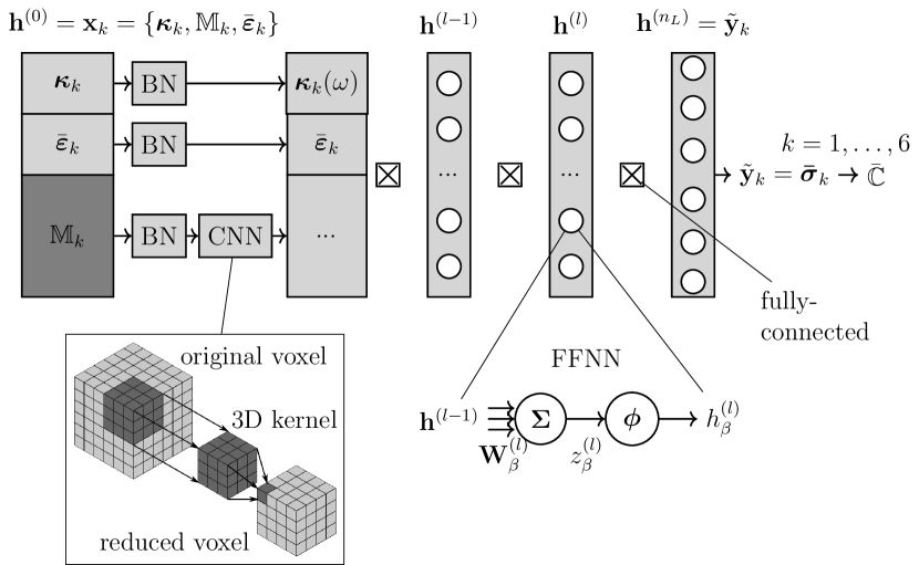
Figure 2: Proposed topology of ANN in Eq. (16) with $n_{L}$ layers $\mathbf{h}^{(l)}$ and $n_{u}$ neural units $h_{\beta}^{(l)}$. An ANN with input ${\mathbf{x}}_{k}=\{\boldsymbol{\kappa}(\omega),\mathbb{M}(\omega),\bar{\boldsymbol{\varepsilon}}\}$, where $\boldsymbol{\kappa}(\omega)$ is a material parameter vector, $\bar{\boldsymbol{\varepsilon}}_{k}$ a macro strain vector and $\mathbb{M}(\omega)$ consist of 3D microstructural voxel data, see Eq. (35). “BN” denotes a batch normalization layer, where the input is standardized, as described in Section 2. $\mathbb{M}(\omega)$ is processed by a CNN in Eq. (19) and after concatenation with $\boldsymbol{\kappa}(\omega)$ and $\bar{\boldsymbol{\varepsilon}}$ feed into an FFNN in Eq. (17). The resulting output is the predicted macroscopic stress tensor $\boldsymbol{\tilde{\bar{\sigma}}}_{k}$ Eq. (47). From six strain states $k$, the macroscopic effective elasticity tensor ${\bar{\boldsymbol{\mathbb{C}}}}$ can be reconstructed as defined in Eq. (48).

(ii) Hyperparameter selection  
Hyperparameters are essential for model performance, i.e. achieving an error in Eq. (21). In this work, hyperparameters of the ANN in Eq. (16) are adjusted by a random search algorithm [53]. A summary of hyperparameters considered in this work is given in Table 2. Hyperparameter tuning is carried out on a separate dataset $\boldsymbol{\mathbb{D}}_{\text{HP}}$, with similar definition as in Eq. (6), to not overfit to the original dataset $\boldsymbol{\mathbb{D}}_{\text{ANN}}$.

Symbol	Description	Reference
$\alpha$	learning rate	Eq. (22)
$\beta$	dropout rate	[41]
$\lambda_{L2}$	L2 parameter	Eq. (21)
$n_{u}$	no. of units (FFNN)	Eq. (17)
$n_{F}$	no. of filters (CNN)	Eq. (19)
$n_{L}$	no. of layers (FFNN)	Eq. (16)

Table 2: Hyperparameters of ANN in Eq. (16) considered in this work.

(iii) Training  
After providing the dataset $\mathbb{D}_{ANN}$ in Algorithm 1 as well as the topology and hyperparameters, the ANN $\tilde{\mathcal{M}}_{ANN}$ is trained by updating its weights Eq. (21) with respect to the dataset $\mathbb{D}_{ANN}$ in Eq. (42). For stochastic gradient descent used to minimize Eq. (22), the ADAM optimizer [54] in its AMSGrad variant [55] is used. The weights $\mathbf{W}$ in Eq. (17) and kernels $\mathbf{K}$ in Eq. (19) are initialized via Glorot Xavier initialization [56]. Early stopping and learning rate decay, as described in [57], are used during optimization Eq. (21).

3.2.4 UQ using pseudospectral PCE and ANN trained on FFT

In Algorithm 3, UQ of the uncertain effective macro elasticity tensor $\bar{\mathbb{C}}(\omega)$ in Eq. (43) using the trained ANN ${\color[rgb]{0,0,0}\tilde{\mathcal{M}}_{ANN}^{t}}$ from Eq. (40) is carried out. For the implementation of pseudospectral PCE as defined in Eq. (7), ChaosPy [58] is used. In the following, the single steps of Algorithm 3 are outlined in detail.

Algorithm 3 : UQ using PCE and ANN trained on FFT

  Input: $\mathbf{X}(\omega)=\{\boldsymbol{\kappa}(\omega),\mathbb{M}(\omega),\bar{\boldsymbol{\varepsilon}}\}\sim\boldsymbol{\mathcal{N}}(\boldsymbol{\mu},\mathbf{\Sigma})$ in Eq. (32)

  Output: $\boldsymbol{\mu}_{\mathbf{Y}},\boldsymbol{\sigma}_{\mathbf{Y}}^{2}$

  

  

  (i) Cubature rule:  Obtain cubature nodes ${\Theta}^{(j)}$ and weights $w({\Theta}^{(j)})$ from Gaussian cubature rule w.r.t. $\mathbf{X}(\omega)$

  

  (ii) Deterministic solutions:  Calculate deterministic solutions at nodes ${\color[rgb]{0,0,0}\mathcal{M}_{\text{ANN}}^{t}({\Theta}^{(j)})}$ in Eq. (9)

  

  (iii) Orthonormal polynomials:  Generate Hermite polynomial ${\Psi}_{\mathbf{i}}$ in Eq. (7)

  

  (iv) PC coefficients:  Calculate PC coefficients ${\color[rgb]{0,0,0}\hat{\mathbb{C}}_{\mathbf{i}}^{ANN}}=\displaystyle\frac{1}{\gamma_{\mathbf{i}}}\displaystyle\sum_{j=1}^{n_{w}}{\color[rgb]{0,0,0}\mathcal{M}_{\text{ANN}}^{t}}(\Theta^{(j)})\Psi_{\mathbf{i}}(\Theta^{(j)})w(\Theta^{(j)})$ in Eq. (41)

  

  (v) Statistics:  Calculate statistics from uncertain effective elasticity tensor   ${\color[rgb]{0,0,0}{\bar{\mathbb{C}}}_{PCE}\approx{\color[rgb]{0,0,0}{\bar{\mathbb{C}}}_{ANN}}(\mathbf{X}(\omega))=\displaystyle\sum_{|\mathbf{i}|\leq n_{PCE}}\hat{\mathbb{C}}_{\mathbf{i}}^{ANN}\Psi_{\mathbf{i}}(\mathbf{\theta}(\omega))}$ in Eq. (43)

Multivariate random input variable  
The random variables $\boldsymbol{\kappa}(\omega)$ in Eq. (28) and $\mathbb{M}(\omega)$ in Eq. (23) from the multivariate random input variable $\mathbf{X}(\omega)$ as defined in Eq. (35) are normally distributed, as seen in the input of Algorithm (3). If multiple material parameters $\boldsymbol{\kappa}(\omega)$ in Eq. (28) are considered, e.g. linear elastic parameters for different constituents as defined in Eq. (28), each individual parameter is a normally distributed univariate random variable. For each univariate random variable of $\mathbf{X}(\omega)$, the mean $\boldsymbol{\mu}$ in Eq. (12) and standard deviation $\boldsymbol{\sigma}$ in Eq. (13) must be provided. ChaosPy [58] then automatically ensembles the corresponding multivariate expectation vector $\boldsymbol{\mu}$, covariance matrix $\mathbf{\Sigma}$ and the multivariate Gaussian distribution $\mathbf{X}(\omega)\sim\boldsymbol{\mathcal{N}}(\boldsymbol{\mu},\mathbf{\Sigma})$, defined by its multivariate CDF. The uncertainty in the microstructure $\mathbb{M}(\omega)$ described in Eq. (23) is defined by its uncertain fiber volume fraction $c_{f}(\omega)$ as seen in Eq. (46) and in this work is considered normally distributed for UQ, i.e. $c_{f}(\omega)\sim\mathcal{N}$.

Remark 3: In practice, the tails of Gaussian distributions lead to physically inadmissible values for the input values in Algorithm 3, as it has support on the entire real line $\mathbb{R}$. To circumvent this problem, in this work truncated Gaussian distributions [59] have been used, which have bounded support. The tails are bounded, where physically meaningfull, i.e. between $0$ and $1$ for the volume fraction $c_{f}(\omega)$ and between $0$ and $0.5$ for the Poisson ratio, for lower and upper bounds, respectively. For the shear modulus $G$ and bulk modulus $K$, only strictly positive values are permitted. Furthermore is is pointed out, that the random variables $\mathbf{X}(\omega)$ used in Algorithm 3 have no connection to the random variables $\mathbf{X}^{U}(\omega)$ used for sampling the training data in Algorithm 1.

(i) Cubature rule  
Since Gaussian random variables are used as input to Algorithm 3, Gauss-Hermite cubature is chosen [60] for numerical integration of Eq. (43) in Algorithm 3.i. ChaosPy [58] uses Stieltjes method on three-term recurrence coefficients for sampling. The order $n_{w}-1$ of the cubature in Eq. (43) must be provided. Nodes ${\Theta}^{(j)}$ and corresponding weights $w(\Theta^{(j)})$ are than chosen automatically with respect to the number of univariate random variables, resulting in a total of $n_{q}$ nodes as defined in Eq. (9).

(ii) Deterministic solutions  
The deterministic solutions for Eq. (43) are carried out on the nodes $\Theta^{(j)}$ by the trained ANN $\tilde{\mathcal{M}}_{ANN}$ in Algorithm 3.ii. For given microstructure $\mathbb{M}(\omega)$ defined in Eq. (23), six strain states are evaluated by the trained ANN $\tilde{\mathcal{M}}_{{ANN}}$, as described in Eq. (48). For uncertain fiber volume fraction $c_{f}(\omega)$ in Eq. (46), for every node $\Theta^{(j)}$ in Eq. (9) a corresponding microstructure is generated synthetically via Section 3.2.2.

(iii) Orthonormal polynomials  
For Gaussian distributions, as in the case of the present work for the input of Algorithm 3, Hermite polynomials $\Psi_{\mathbf{i}}$ are used in Eq. (39). The polynomial degree $n_{PCE}$ in Eq. (7) must be provided. Then, Polynomials are generated by three-term recurrence described in [38].

(iv) PC coefficients  
The PC coefficients ${\color[rgb]{0,0,0}\hat{\mathbb{C}}_{\mathbf{i}}^{ANN}}$ in Eq. (43) are then calculated by Algorithm (3.iv). With the calculated PC coefficients ${\color[rgb]{0,0,0}\hat{\mathbb{C}}_{\mathbf{i}}^{ANN}}$ and the orthonormal polynomials $\Psi_{\mathbf{i}}$, the uncertain effective macro elasticity tensor ${\color[rgb]{0,0,0}\bar{\mathbb{C}}_{ANN}(\omega)}$ is fully defined by Eq. (43).

(v) Statistics  
The central moments like mean $\boldsymbol{\mu}_{\mathbf{Y}}$ in Eq. (14) and standard deviation $\boldsymbol{\sigma}_{\mathbf{Y}}$ in Eq. (15) of ${\color[rgb]{0,0,0}\bar{\mathbb{C}}_{ANN}(\omega)}$ in Eq. (43) can then be obtained from the PC coefficients ${\color[rgb]{0,0,0}\hat{\mathbb{C}}_{\mathbf{i}}^{ANN}}$ Eq. (43), which is carried out by ChaosPy [58]. Corresponding PDF and CDF can be reconstructed by kernel density estimators [58].

4 Numerical examples

4.1 Example 1: effective transversely isotropic properties of carbon fiber reinforced polymer

4.1.1 Problem description

The first example compares the proposed method in Section 3 with a different uncertain homogenization approach from the literature. In [19], the authors investigate a single long fiber inclusion centered in a matrix material, where the cubic representative volume element with unit dimensions $\xi_{i}$ in Eq. (23) is shown in Figure 3a. Here, deterministic fiber material parameters $\boldsymbol{\kappa}^{I}$ and uncertain, normally distributed matrix material parameters $\boldsymbol{\kappa}^{M}(\omega)\sim\boldsymbol{\mathcal{N}}(\boldsymbol{\mu},\boldsymbol{\sigma}^{2})$ in Eq. (28) are considered. Additionally, uncertainty in the geometry is studied by employing an uncertain, normally distributed fiber volume fraction $c_{f}(\omega)\sim\mathcal{N}(\boldsymbol{\mu},\boldsymbol{\sigma}^{2})$ of the microstructure $\mathbb{M}(\omega)$ in Eq. (23), effectively altering the radius of the fiber inclusion. The normal distributions $\boldsymbol{\mathcal{N}}(\boldsymbol{\mu},\boldsymbol{\sigma}^{2})$ are fully defined by their mean values $\boldsymbol{\mu}_{\mathbf{X}}$ in Eq. (12) and standard deviations $\boldsymbol{\sigma}_{\mathbf{X}}$ in Eq. (13). Given uncertain linear elastic isotropic material parameters of single constituents in Table 3, uncertain effective transversal isotropic properties $\bar{E}_{1}(\omega),\bar{E}_{2}(\omega),\bar{G}_{12}(\omega),\bar{G}_{23}(\omega),\bar{\nu}_{12}(\omega),\bar{\nu}_{23}(\omega)$ calculated from ${\color[rgb]{0,0,0}\bar{\mathbb{C}}_{ANN}(\omega)}$ in Eq. (43) are of interest

$$\bar{\mathbb{C}}(\omega)\xrightarrow{\text{Voigt}}\underline{\underline{\bar{\mathbb{C}}}}(\omega)=\left[\begin{array}[]{cccccc}\bar{\mathbb{C}}_{1111}&2\bar{\nu}_{12}\left(\bar{\lambda}+\bar{G}_{23}\right)&2\bar{\nu}_{12}\left(\bar{\lambda}+\bar{G}_{23}\right)&0&0&0\\ &\bar{\lambda}+2\bar{G}_{23}&\bar{\lambda}&0&0&0\\ &&\bar{\lambda}+2\bar{G}_{23}&0&0&0\\ &&&\bar{G}_{23}&0&0\\ &\text{ sym. }&&&\bar{G}_{12}&0\\ &&&&&\bar{G}_{12}\end{array}\right]$$ ((50))

$$\bar{\mathbb{C}}_{1111}=\frac{1-\bar{\nu}_{23}}{1-\bar{\nu}_{23}-2\bar{\nu}_{12}\bar{\nu}_{21}}\bar{E}_{1},\qquad\bar{\lambda}=\frac{\bar{\nu}_{12}\bar{\nu}_{21}+\bar{\nu}_{23}}{\left(1-\bar{\nu}_{23}-2\bar{\nu}_{12}\bar{\nu}_{21}\right)\left(1+\bar{\nu}_{23}\right)}\bar{E}_{2}$$

where the elementary event $\omega$ in Eq. (1) applies to all variables, but is omitted for readability. In [19], a Galerkin PCE with FEM for uncertain full-field homogenization of the representative volume element shown in Figure 3a is utilized. Periodic boundary conditions are used, as explained in Eq. (26).

In the following, the results from [19] are used as comparison to the proposed approach in Section 3. The input values in Table 3 are the same as in [19].

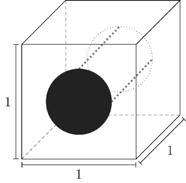
(a)

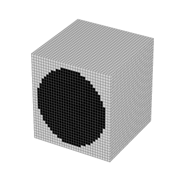
(b)

Figure 3: Example 1: (a) Geometry of a long fiber inclusion centered in a matrix material. (b) Voxel discretization using 32 voxels per dimension.

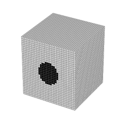
(a)

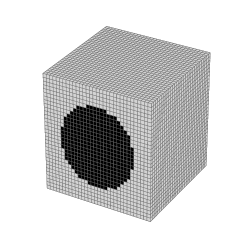
(b)

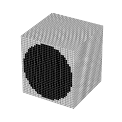
(c)

Figure 4: Example 1: Geometry of a long fiber inclusion centered in a matrix material for different fiber volume fractions $c_{f}$ in Eq. (46). (a) $c_{f}=0.1$, (b) $c_{f}=0.4$, (c) $c_{f}=0.7$.

Parameters of $\mathcal{N}(\boldsymbol{\mu}_{\mathbf{X}},\boldsymbol{\sigma}_{\mathbf{X}}^{2})$	$c_{f}(\omega)$ [-]	$E^{M}(\omega)[\text{MPa}]$	$\nu^{M}(\omega)$ [-]	$E^{I}[\text{MPa}]$	$\nu^{I}$ [-]
$\boldsymbol{\mu}_{\mathbf{X}}$	$0.6335$	$3.101\times 10^{3}$	$0.41$	$2.31\times 10^{5}$	$0.1$
$\boldsymbol{\sigma}_{\mathbf{X}}$	$0.0264$	$1.11\times 10^{2}$	$0.044$	-	-

Table 3: Example 1: Parameters for the normally distributed input random variable $\mathbf{X}(\omega)\sim\boldsymbol{\mathcal{N}}(\boldsymbol{\mu}_{\mathbf{X}},\boldsymbol{\sigma}_{\mathbf{X}}^{2})$ of the dataset $\mathbb{D}_{ANN}$ according to the input of Algorithm 3 and Eq. (14), Eq. (15).

4.1.2 Data generation for deep learning using FFT

Following Section 3.2.2 and Algorithm 1, a dataset $\mathbb{D}_{ANN}$ as defined in Eq. (42) is created. Here, $n_{s}=9000$ three dimensional microstructures $\mathbb{M}(\omega)$ in Eq. (23), discretized by voxels as shown in Figure 4a - (c), are homogenized by FFT on a computer cluster. The uniform distributions from Table 4 are used for sampling the inputs $c_{f}$ and $\boldsymbol{\kappa}^{M}=\{E^{M},\nu^{M}\}$, where the fiber parameters $\boldsymbol{\kappa}^{I}$ are fixed. The upper and lower boundaries $a$ and $b$, respectively, are chosen with physical constraints in mind as explained in Eq. (45).

Remark 4: If the fiber volume fraction $c_{f}$ approaches 1, the stiffness of the microstructure will be identical to the deterministic stiffness of the fiber. For $c_{f}$ close to 1, overlapping of the fiber can appear. This unphysical behavior can be avoided by carefully choosing the fiber volume fraction in the stochastic analysis in Section 4.1.3 , which should be well below 1.

Parameters of $\mathcal{U}(\underline{x},\bar{x})$	$c_{f}$ [-]	$E^{M}[\text{MPa}]$	$\nu^{M}$ [-]
$\underline{x}$	0	$10^{3}$	0.1
$\bar{x}$	1	$10^{4}$	0.48

Table 4: Example 1: Uniform distributions with lower and upper limit $(a,b)$, respectively, of training samples $\mathbf{x}_{k}$ according to Eq. (44).

4.1.3 ANN design and training

An ANN is created following Section 3.2.3, Algorithm 3 and according to the topology outlined in Figure 2. For the CNN in Figure 2, an AlexNet is chosen, as described in Section 2.(i). The hyperparameters of the ANN according to Table 2 are chosen by random search following Section 2.(ii). The optimized values, which give the lowest error on a corresponding dataset $\mathbb{D}_{HP}$, are given in Table 5. The mean relative error after training with respect to a test set using these hyperparameters is $2.54\%$.

Symbol	$\alpha$	$\beta$	$\lambda_{L2}$	$n_{u}$	$n_{F}$	$n_{L}$
Optimized value	0.005	0.0	0.0	2048	32	2

Table 5: Example 1: Optimized values for hyperparameters of the ANN from Table 2 with respect to the error function in Eq. (21), which lead to the lowest error $\mathcal{E}$.

4.1.4 UQ using PCE and ANN trained on FFT

After training of the ANN $\tilde{\mathcal{M}}_{ANN}$ in the previous section, UQ is carried out following Section 3.2.4 and Algorithm 3. The sample distributions of the input parameters $\mathbf{X}(\omega)$ in Algorithm 3 are according to [19], which are outlined in Table 3. Consequently, the dimension $n_{x}$ of the random input space $\mathcal{D}_{\mathbf{X}}$ is $n_{x}=|\{c_{f}(\omega),E^{M}(\omega),\nu^{M}(\omega)\}|=3$. For integration a Gaussian multivariate cubature of order $n_{w}-1=9$ in Eq. (10) is chosen. The calculations of ${\color[rgb]{0,0,0}n_{q}}=(n_{w}=10)^{n_{x}=3}=10^{3}$ deterministic solutions in Eq. (43) are carried out by the trained ANN ${\color[rgb]{0,0,0}\tilde{\mathcal{M}}_{ANN}^{t}}$. Hermite polynomials $\Psi_{\mathbf{i}}$ with order $n_{PCE}=9$ are used as polynomial basis in Eq. (7). The PC coefficients $\hat{\mathbb{C}}_{\mathbf{i}}$ are then calculated by pseudospectral PCE defined in Eq. (7).

The resulting CDFs defined in Eq. (7) of the uncertain effective transversal isotropic properties $\bar{E}_{1}(\omega),\bar{E}_{2}(\omega),\bar{G}_{12}(\omega),\bar{G}_{23}(\omega),\bar{\nu}_{12}(\omega),\bar{\nu}_{23}(\omega)$ in Eq. (50) of the uncertain effective elasticity tensor ${\color[rgb]{0,0,0}\bar{\mathbb{C}}_{ANN}(\omega)}$ in Eq. (43) are shown in Figure 5. The solutions of the proposed algorithm are denoted by ANN whereas the reference solutions obtained by [19] using FEM are denoted by FE. Between these two methods, an agreement of the corresponding CDFs can be observed. It has to be mentioned, that deviations in CDFs can be more pronounced in PDFs. For consistency with [19] as well as unified presentation, in this work CDFs were chosen to display results. Deviations can be explained by multiple factors. First, the voxel discretization shown in 3b differs from the finite element discretization in [19]. As can be seen in Figure 4a - c, circular geometries are only approximated voxels, resulting in stair-like effects. These differences lead to perturbations in the micro stress field $\boldsymbol{\sigma}(\omega)$ in Eq. (25), which ultimately influence the effective macro properties of the uncertain effective elasticity tensor $\bar{\mathbb{C}}(\omega)$ in Eq. (43) using Eq. (48) utilizing FFT in Eq. (34). Second, the approximation error of the ANN in Eq. (21) leads to errors in the deterministic solution ${\color[rgb]{0,0,0}\tilde{\mathcal{M}}_{\text{ANN}}^{t}}$ of Eq. (43). Third, the pseudospectral approach of PCE in Eq. (10) inherits a number of approximations contributing to the overall deviations between both homogenization approaches, namely usage of cubature and different polynomial orders of the orthonormal polynomials in Eq. (7).

Despite the minor deviations in the CDFs, the proposed algorithm is capable of predicting the uncertain effective properties of transversely isotropic fiber reinforced materials.

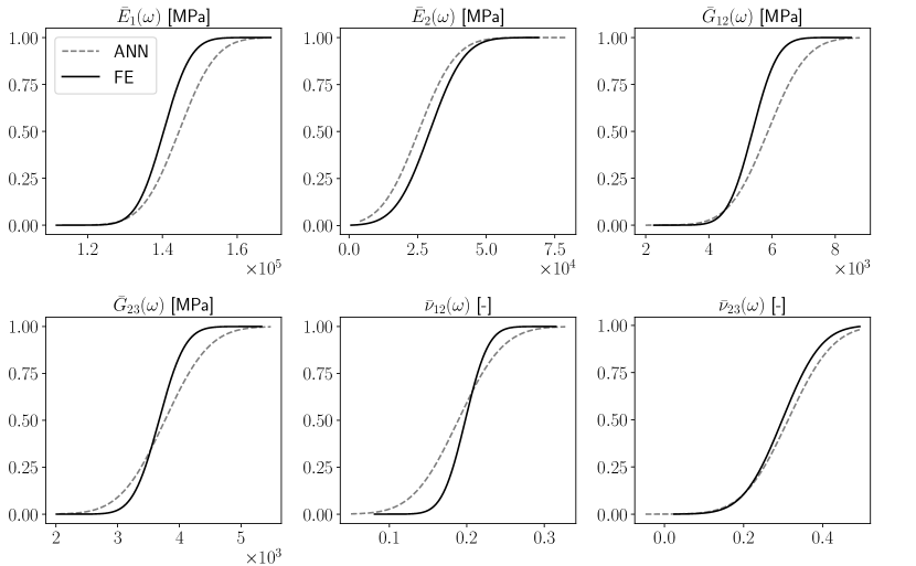
(a)

Figure 5: Example 1: Comparison of CDFs of uncertain effective transversal isotropic properties $\bar{E}_{1}(\omega),\bar{E}_{2}(\omega),\bar{G}_{12}(\omega),\bar{G}_{23}(\omega),\bar{\nu}_{12}(\omega),\bar{\nu}_{23}(\omega)$ in Eq. (50) of the ANN model (ANN) and the finite element reference solution by [19] (FE).

4.2 Example 2: effective isotropic properties of spherical inclusions

4.2.1 Problem description

The second example deals with more complex microstructure compared to Example 1. A cubical unit cell consisting of matrix material with multiple spherical inclusions, as shown in Figure 6b, is considered. The performance of the proposed method is compared to MC simulations of a deterministic FFT solver, in particular the speed up of the ANN approach is investigated. Additionally, to compare the error induced by the PCE, MC simulations using the ANN solver are carried out. In this example, the Matrix material parameters $\boldsymbol{\kappa}^{M}(\omega)$ in Eq. (28) are normally distributed random variables. The corresponding parameters are shown in Table 6. The parameters of the inclusion material $\boldsymbol{\kappa}^{I}$ are considered to be deterministic. Uncertainty of the geometry is taken into account by a normally distributed inclusion volume fraction $c_{f}(\omega)\sim\mathcal{N}(\boldsymbol{\mu},\boldsymbol{\sigma}^{2})$ of the microstructure $\mathbb{M}(\omega)$ in Eq. (23). This inclusion volume fraction then determines the number of spherical inclusions. Normal distributions $\mathcal{N}(\boldsymbol{\mu}_{\mathbf{X}},\boldsymbol{\sigma}_{\mathbf{X}}^{2})$ again are completely defined by Eq. (12) and Eq. (13). Because of the random placement of the spherical inclusions, the macroscopic material behaviour is assumed to be isotropic. Therefore, uncertain effective linear elastic isotropic properties $\bar{E}(\omega),\bar{\nu}(\omega)$ calculated from ${\color[rgb]{0,0,0}\bar{\mathbb{C}}_{ANN}(\omega)}$ in Eq. (43) are of interest

$$\bar{\mathbb{C}}(\omega)\xrightarrow{\text{Voigt}}\underline{\underline{\bar{\mathbb{C}}}}(\omega)=\left[\begin{array}[]{cccccc}2\bar{\mu}+\bar{\lambda}&\bar{\lambda}&\bar{\lambda}&0&0&0\\ &2\bar{\mu}+\bar{\lambda}&\bar{\lambda}&0&0&0\\ &&2\bar{\mu}+\bar{\lambda}&0&0&0\\ &&&\bar{\mu}&0&0\\ &\text{sym.}&&&\bar{\mu}&0\\ &&&&&\bar{\mu}\end{array}\right]$$ ((51))

$$\bar{\mu}=\frac{\bar{E}}{2(1+\bar{\nu})},\qquad\bar{\lambda}=\frac{\bar{E}\bar{\nu}}{(1+\bar{\nu})(1-2\bar{\nu})}$$

where the elementary event $\omega$ Eq. (1) applies to all variables but is omitted for readability. Deviations from the isotropic form in Section 4.2.1 are neglected. For the reference MC simulations using the FFT solver, the number of samples is chosen as $n_{s}=10^{3}$. This number of simulations is sufficient for mean and standard deviation estimation as mentioned by [7]. For the MC simulations using the ANN solver, the number of samples is chosen as $n_{s}=10^{4}$.

Remark 5: The ANN has to be trained only once. After that, a deterministic surrogate for the FFT solver has been established, which can be used for multiple stochastic investigations. The computational effort is one time only and is front loaded. As the sample generation is pleasingly parallel, it is well suited for computation on cluster computers. After training, the ANN is much faster than the original FFT solver, as can be seen Figure 9.

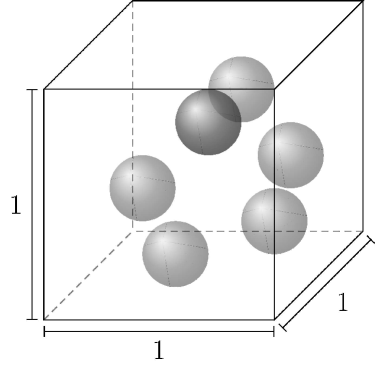
(a)

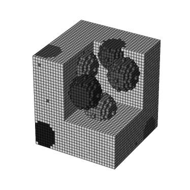
(b)

Figure 6: Example 1: (a) Geometry of multiple spherical inclusion embedded in a matrix material. (b) Voxel discretization using 32 voxels per dimension.

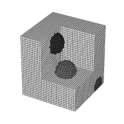
(a)

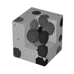
(b)

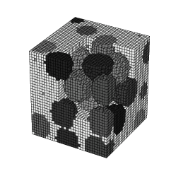
(c)

Figure 7: Example 1: Geometry of multiple spherical inclusion embedded in a matrix material for different inclusion volume fractions $c_{f}$ in Eq. (46). (a) $c_{f}=0.05$. (b) $c_{f}=0.3$. (c) $c_{f}=0.4$.

Parameters of $\mathcal{N}(\boldsymbol{\mu}_{\mathbf{X}},\boldsymbol{\sigma}_{\mathbf{X}}^{2})$	$c_{f}(\omega)$ [-]	$E^{M}(\omega)[\text{MPa}]$	$\nu^{M}(\omega)$ [-]	$E^{I}[\text{MPa}]$	$\nu^{I}$ [-]
$\boldsymbol{\mu}_{\mathbf{X}}$	$0.2$	$5\times 10^{3}$	$0.3$	$2.31\times 10^{5}$	$0.1$
$\boldsymbol{\sigma}_{\mathbf{X}}$	$0.02$	$5\times 10^{2}$	$0.03$	-	-

Table 6: Example 2: Parameters for the normally distributed input random variables $\mathbf{X}(\omega)\sim\mathcal{N}(\boldsymbol{\mu}_{\mathbf{X}},\boldsymbol{\sigma}_{\mathbf{X}}^{2})$ of the dataset $\mathbb{D}_{ANN}$ according to the input of Algorithm 3 and Eq. (14), Eq. (15).

4.2.2 Data generation for deep learning using FFT

Following Section 3.2.2 and Algorithm 1, a dataset $\mathbb{D}_{ANN}$ defined in Eq. (42) with $n_{s}=13800$ three dimensional microstructures $\mathbb{M}$ from Eq. (23), discretized by voxels as shown in Figure 7a - c, is homogenized by FFT as defined in Eq. (34) on a computer cluster. The uniform distributions from Table 7 are used for sampling the inputs $c_{f},E^{M}$ and $\nu^{M}$, where the inclusion parameters $\boldsymbol{\kappa}^{I}$ are fixed. The upper and lower boundaries $a$ and $b$, respectively, are chosen with physical constraints in mind as explained in Eq. (45). During microstructure generation, overlap of particles is avoided by the algorithm by rejecting spherical inclusion, where shared voxels with already placed particles are detected.

4.2.3 ANN design and training

An ANN is created following Section 3.2.3 and Algorithm 3, where the topology is shown in Figure 2. In contrast to Example 1, for the CNN in Figure 2, a 40-layer DenseNet is chosen to account for the more complex microstructure as described in Section 2. The hyperparameters of ANN according to Table 2 are chosen by random search, similarly as for Example 1. The optimal values for the topology chosen are given in Table 8. The mean-relative error with respect to a test set is 4.0%. This higher error is explained by the more complex microstructure as well as the choice of CNN, which is deeper and therefore more difficult to train. Nevertheless, the DenseNet performed better than AlexNet for the microstructure considered, although this comparison is not shown in the present work.

Parameters of $\mathcal{U}(\underline{x},\bar{x})$	$c_{f}$ [-]	$E^{M}[\text{MPa}]$	$\nu^{M}(\omega)$ [-]
$\underline{x}$	0	$10^{3}$	0.1
$\bar{x}$	0.4	$10^{4}$	0.48

Table 7: Example 2: Uniform distributions with lower and upper limit $a$ and $b$, respectively, of training samples $\mathbf{x}_{k}$ according to Eq. (44).

Symbol	$\alpha$	$\beta$	$\lambda_{L2}$	$n_{u}$	$n_{F}$	$n_{L}$
Optimum	0.01	0.15	$10^{-4}$	1024	-	2

Table 8: Example 2: Optimized values for hyperparameters of the ANN from Table 2 with respect to the error function in Eq. (21), which lead to the lowest error $\mathcal{E}$.

4.2.4 UQ using PCE and ANN trained on FFT

The UQ is carried out similarly to the procedure in Example 1. Following Section 3.2.4 and Algorithm 3, first the sample distributions of the multivariate random input variables ${\mathbf{x}}_{k}=\left\{\boldsymbol{\mathbb{M}},\boldsymbol{\kappa},\bar{\underline{\boldsymbol{\varepsilon}}}\right\}$ in the input of Algorithm 3 are chosen according to Table 6. A Gaussian multivariate cubature of order $n_{w}-1=9$ in Eq. (10) is chosen. Deterministic solutions are provided by the trained ANN ${\color[rgb]{0,0,0}\tilde{\mathcal{M}}_{ANN}^{t}}$ in Eq. (43). Hermite polynomials with order $n_{PCE}=9$ are used as defined in Eq. (7). The PC coefficients ${\color[rgb]{0,0,0}\hat{\mathbb{C}}^{ANN}_{\mathbf{i}}}$ are calculated by pseudospectral PCE defined in Eq. (7). The CDFs of the uncertain effective linear elastic isotropic properties $\bar{E}(\omega),\bar{\nu}(\omega)$ from Section 4.2.1 of the uncertain effective elasticity tensor ${\color[rgb]{0,0,0}\bar{\mathbb{C}}_{ANN}(\omega)}$ from Eq. (43) are shown in Figure 8. The solution from the ANN using PCE is denoted by PCE ANN while the reference solution from MC simulations using the FFT solver is denoted by MC FFT. The solution from MC simulations using the ANN solver is denoted by MC ANN.

The comparison of the CDFs between the proposed method and the reference is shown in Figure 8. The results indicate, that the presented method is capable of predicting uncertain effective properties for complex microstructures consisting of matrix material and spherical, randomly distributed spherical inclusions. The deviations can be explained similarly to Example 1. For Example 2, the approximation error of the network is larger than in the case of single fiber inclusions. Again, the usage of cubature and polynomial expansion in the PCE yield further error sources, but these are minor, as comparisons of the ANN using PCE and the ANN using MC in Figure 8 indicate. The mean values for both effective properties show close correspondence to the reference FFT solution, while their respective variances differ. The asymmetrical CDF with respect to the Poisson’s ratio $\bar{\nu}(\omega)$ in Figure 8 indicates, that the network accuracy alters for certain values.

Beside the accuracy comparison, the computation time for a full homogenization is investigated in Figure 9. The evaluation time on a mobile workstation with Nvidia M5000M GPU for the deterministic FFT used by the MC reference solution and the ANN is plotted against the number of voxels. Both methods use GPU acceleration, the FFT algorithm utilizes CuPy [61] and the ANN algorithm Tensorflow [44]. It can be seen, that the ANN approach is magnitudes faster than FFT. Furthermore, the scaling and memory efficiency of the ANN with respect to the number of used voxels is better than in the case of FFT. Using e.g. $\xi_{1}=\xi_{2}=\xi_{3}=128^{3}$ voxels from Eq. (23) yields the memory limit for the FFT approach on the 8 GB GPU, whereas the ANN is capable of processing up to $\xi_{1}=\xi_{2}=\xi_{3}=256^{3}$ voxels. With this speed up it is possible to carry out uncertain computations without a large scale computer cluster system.

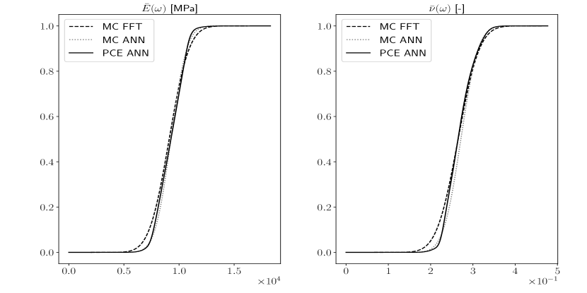
(a)

Figure 8: Example 2: Comparison of CDFs of uncertain effective linear elastic isotropic properties $\bar{E}(\omega),\bar{\nu}(\omega)$ of the ANN model using PCE (PCE ANN), the ANN model using $10^{4}$ MC simulations and $10^{3}$ MC simulations of the FFT solver (MC FFT).

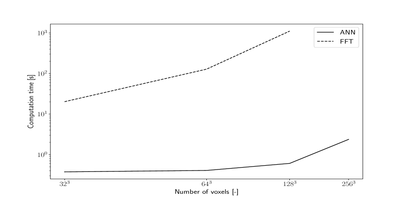
(a)

Figure 9: Example 2: Comparison of computation time for full homogenization in six strain directions of the ANN model (ANN) with FFT (FFT). For FFT, there are no results for unit cells larger than $\xi_{1}=\xi_{2}=\xi_{3}=128^{3}$ voxels per dimension, as defined in Eq. (23), due to memory limitations of the GPU. All computations were carried out on a mobile workstation with Nvidia M5000M GPU.

4.3 Example 3: effective transversely isotropic properties of carbon fiber reinforced polymer with ANN trained on spherical inclusions

4.3.1 Problem description

In Example 3, the ANN from Example 4.2, which is trained on spherical inclusions in Figure 6b, is tested on the microstructure from Example 4.1, which are cylindrical single fiber inclusions, seen in Figure 3b. The cylindrical single fiber inclusions inherits transversely isotropic macroscopic material behaviour, while the spherical inclusions are isotropic. The aim of this example is to investigate the generalization behaviour of the ANN with respect to different microstructures. As can be seen in Figure 10, large deviations of the ANN predictions to the finite element reference solution are present. The ANN trained on spherical inclusions with isotropic material behaviour is not able to capture the transversely isotropic behaviour of the single fiber inclusions. This indicates, that the ANN is only capable to homogenize microstructures it is trained on.

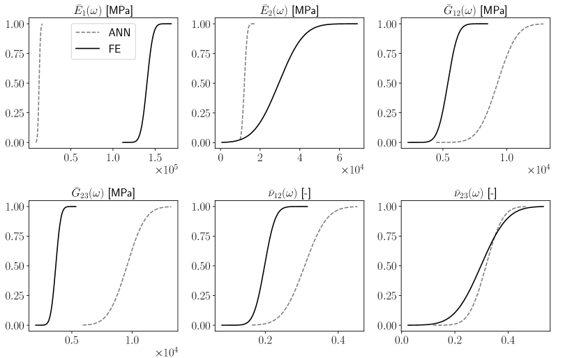
(a)

Figure 10: Example 3: Comparison of CDFs of ANN model (ANN) trained on spherical inclusions from Example 2 and [19] (FE).

To investigate the performance on a mixed set with respect to the underlying microstructure, the two datasets from Example 1 and Example 2, in the following denoted by $\mathbb{D}_{ANN}^{(1)}$ and $\mathbb{D}_{ANN}^{(2)}$, respectively, are simply combined, such that

$$\mathbb{D}_{ANN}=\mathbb{D}_{ANN}^{(1)}+\mathbb{D}_{ANN}^{(2)}$$

in an appropriate sense. Then, keeping the hyperparameters and topology of the ANN the same as in Example 2, namely adopting the hyperparameters in Table 8 and utilizing a Densenet for the CNN, the ANN is trained on the mixed set $\mathbb{D}_{ANN}$. After training, UQ is carried out twice, once with respect to the configurations in Example 1 and once with respect to the configurations in Example 2. The resulting CDFs are shown in Figure 11 and Figure 12, respectively.

First consider the results from Figure 11. Here, the predictions with respect to the single fiber microstructure from Example 1 of the ANN trained on the mixed set are shown. Compared to Figure 10, where the ANN is trained on spherical inclusions, the results have improved and show better agreement with the reference solution. The quality of the outcomes, i.e. the overlap between ANN and reference solution, are even comparable with the results from Example 1 in Figure 5, where the ANN is trained purely on single fibers. The results indicate that the ANN is able to correctly identify the nature of the microstructure, given that it is included in the training set.

Second consider the results from Figure 12. Here the predictions with respect to the spherical inclusion microstructure from Example 2 of the ANN trained on the mixed set is shown. Deviations of the macroscopic Young’s modulus can be observed and the predictive capability is worse in comparison with the ANN from Example 2, which was trained purely on spherical microstructures.

The authors are aware of this discrepancy, as it is expected for the ANN to perform better on microstructures, for which more samples are available in the training dataset. Currently, no solution to this open problem is available.

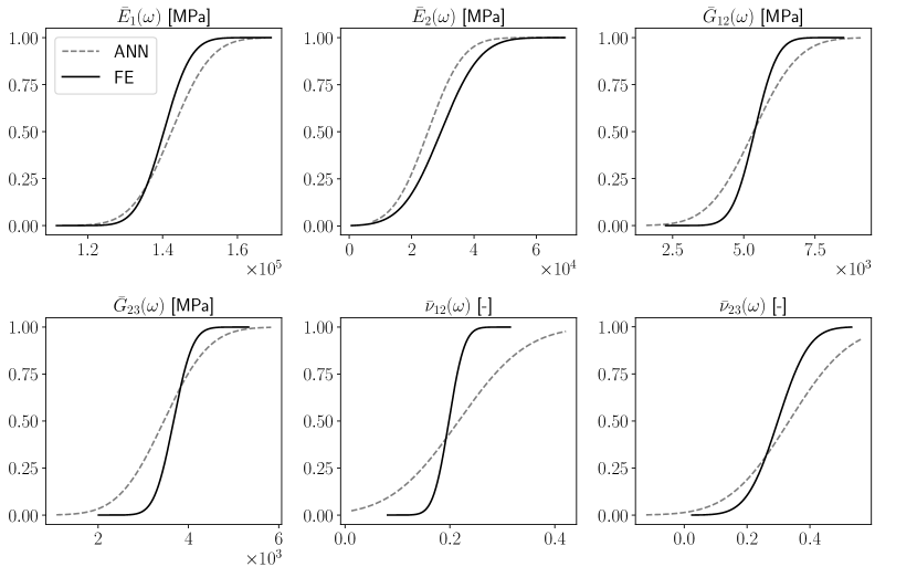
(a)

Figure 11: Example 3: Comparison of CDFs of ANN model (ANN) trained on single fiber and spherical inclusions from Example 1 and Example 2, respectively, and [19] (FE).

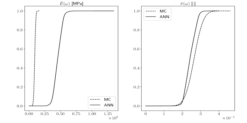
(a)

Figure 12: Example 3: Comparison of CDFs of ANN model (ANN) trained on single fiber and spherical inclusions from Example 1 and Example 2, respectively, and $10^{3}$ MC simulations.

5 Conclusion and outlook

The objective of this paper is to present a deep learning driven pseudospectral PCE based FFT homogenization algorithm in order to quantify efficiently uncertainties in effective properties of complex, three dimensional microstructures. Here, uncertainties arising from material parameters of single constituents as well as the geometry of the underlying microstructure were considered. In order to reduce the computational effort of uncertain full-field homogenization, which is commonly treated by FEM discretization and MC methods, a deep learning algorithm is proposed. The ANN is trained on FFT homogenized samples to circumvent meshing, which leads to a deterministic surrogate. Then, by usage of pseudospectral PCE, a stochastic surrogate is established, capable of predicting uncertain effective properties in multiple loading directions. Therefore, the proposed approach is able to calculate the full uncertain effective elasticity tensor.

Several examples were given. The first example shows the ability of the proposed algorithm to predict uncertain effective properties of transversely linear elastic carbon fiber reinforced polymers by comparing it to established methods from the literature. Here, the presented results indicate a good agreement with [19]. The second example expands the method further to complex microstructures, comparing MC of FFT and with the proposed PCE/ANN algorithm. Again, the proposed algorithm is capable of predicting uncertain effective properties. It is shown, that the error induced from the PCE is small in comparison with MC, indicating that the main error source is the error by the ANN. Additionally, a significant speed up in the deterministic solution by the ANN compared to FFT was reported. The third example shows the problem of generalization of the ANN predictions. Here, an ANN trained sole on one type of microstructure was not able to transfer the knowledge to other microstructures. This means, that if one wants general prediction capabilities, a broad family of diverse microstructures have to be included in the training set during training stage. This could lead to large training sets, as for every type of microstructure thousands of different samples are needed. While the proposed approach is well suited for a specific family of microstructures, which are included in the training stage, recent developments in operator learning [62] could permit more generalization power, as reported in e.g. [63] and [64].

Compared to different approaches in the literature, this algorithm is capable of predicting effective properties projected to uncertainties of material parameters and geometry in three dimensional microstructures, were attempts in the literature were restricted to either deterministic approaches, two dimensions, fixed material parameters or a single loading direction.

The proposed approach enabled full-field uncertainty quantification by building an efficient surrogate based on deep learning. Here, the computational heavy part is front loaded in the sense, that the single model evaluation is cheap in comparison to FEM or FFT, but the training, or preprocessing, is more involved, which on the other hand, is only a one time effort. Nevertheless, the reduction of sample generation and training time is an important topic for future work. An interesting approach in this context is the utilization of so called physics informed neural networks [65], which solve the underlying system of partial differential equations directly, effectively bypassing the need of sample creation and label generation. An intrusive Galerkin projection, as presented in [19], could be a possibility to include uncertainties in such an approach. Furthermore, real world examples, such as complex microstructures from CT-scans, and experimental data are needed to validate the proposed method.

References

- [1] J. Aboudi, S. M. Arnold, B. A. Bednarcyk, Micromechanics of composite materials: a generalized multiscale analysis approach, Butterworth-Heinemann, 2012.
- [2] H. J. Böhm, A short introduction to continuum micromechanics, in: Mechanics of microstructured materials, Springer, 2004, pp. 1–40.
- [3] V. Müller, M. Kabel, H. Andrä, T. Böhlke, Homogenization of linear elastic properties of short-fiber reinforced composites–a comparison of mean field and voxel-based methods, International Journal of Solids and Structures 67 (2015) 56–70.
- [4] M. C. Kennedy, A. O’Hagan, Bayesian calibration of computer models, Journal of the Royal Statistical Society: Series B (Statistical Methodology) 63 (3) (2001) 425–464.
- [5] A. Der Kiureghian, O. Ditlevsen, Aleatory or epistemic? does it matter?, Structural safety 31 (2) (2009) 105–112.
- [6] B. Hiriyur, H. Waisman, G. Deodatis, Uncertainty quantification in homogenization of heterogeneous microstructures modeled by xfem, International Journal for Numerical Methods in Engineering 88 (3) (2011) 257–278.
-
[7]
B. Sudret, S. Marelli, J. Wiart,
Surrogate models for
uncertainty quantification: An overview, in: 2017 11th European
Conference on Antennas and Propagation (EUCAP), IEEE, Paris, France,
2017, pp. 793–797.
doi:10.23919/EuCAP.2017.7928679.
URL http://ieeexplore.ieee.org/document/7928679/ -
[8]
J. E. Hurtado, A. H. Barbat, Monte
Carlo techniques in computational stochastic mechanics, Archives of
Computational Methods in Engineering 5 (1) (1998) 3.
doi:10.1007/BF02736747.
URL https://doi.org/10.1007/BF02736747 - [9] R. E. Caflisch, et al., Monte carlo and quasi-monte carlo methods, Acta numerica 1998 (1998) 1–49.
- [10] R. G. Ghanem, P. D. Spanos, Stochastic Finite Elements: A Spectral Approach, Courier Corporation, 2003.
-
[11]
D. Xiu, G. E. Karniadakis,
The
Wiener–Askey Polynomial Chaos for Stochastic Differential
Equations, SIAM Journal on Scientific Computing 24 (2) (2002) 619–644.
doi:10.1137/S1064827501387826.
URL https://epubs.siam.org/doi/abs/10.1137/S1064827501387826 - [12] J. Vondřejc, D. Liu, M. Ladeckỳ, H. G. Matthies, Fft-based homogenisation accelerated by low-rank tensor approximations, Computer Methods in Applied Mechanics and Engineering 364 (2020) 112890.
- [13] C. Soize, Tensor-valued random fields for meso-scale stochastic model of anisotropic elastic microstructure and probabilistic analysis of representative volume element size, Probabilistic Engineering Mechanics 23 (2-3) (2008) 307–323.
- [14] R. Cottereau, D. Clouteau, H. B. Dhia, Localized modeling of uncertainty in the arlequin framework, in: IUTAM Symposium on the Vibration Analysis of Structures with Uncertainties, Springer, 2011, pp. 457–468.
- [15] A. Noshadravan, R. Ghanem, J. Guilleminot, I. Atodaria, P. Peralta, Validation of a probabilistic model for mesoscale elasticity tensor of random polycrystals, International Journal for Uncertainty Quantification 3 (1) (2013) 73–100.
- [16] J. Guilleminot, C. Soize, Stochastic model and generator for random fields with symmetry properties: application to the mesoscopic modeling of elastic random media, Multiscale Modeling & Simulation 11 (3) (2013) 840–870.
- [17] A. Clément, C. Soize, J. Yvonnet, Uncertainty quantification in computational stochastic multiscale analysis of nonlinear elastic materials, Computer Methods in Applied Mechanics and Engineering 254 (2013) 61–82.
- [18] M. Tootkaboni, L. Graham-Brady, A multi-scale spectral stochastic method for homogenization of multi-phase periodic composites with random material properties, International journal for numerical methods in engineering 83 (1) (2010) 59–90.
-
[19]
I. Caylak, E. Penner, R. Mahnken,
Mean-field
and full-field homogenization with polymorphic uncertain geometry and
material parameters, Computer Methods in Applied Mechanics and Engineering
373 (2021) 113439.
doi:https://doi.org/10.1016/j.cma.2020.113439.
URL http://www.sciencedirect.com/science/article/pii/S0045782520306241 -
[20]
C. Miehe, A. Koch,
Computational
micro-to-macro transitions of discretized microstructures undergoing small
strains, Archive of Applied Mechanics (Ingenieur Archiv) 72 (4-5) (2002)
300–317.
doi:10.1007/s00419-002-0212-2.
URL http://link.springer.com/10.1007/s00419-002-0212-2 - [21] B. J. Debusschere, H. N. Najm, P. P. Pébay, O. M. Knio, R. G. Ghanem, O. P. Le Maitre, Numerical challenges in the use of polynomial chaos representations for stochastic processes, SIAM journal on scientific computing 26 (2) (2004) 698–719.
- [22] M. Schneider, A review of nonlinear fft-based computational homogenization methods, Acta Mechanica (2021) 1–50.
- [23] H. Moulinec, P. Suquet, A FFT-Based Numerical Method for Computing the Mechanical Properties of Composites from Images of their Microstructures, in: R. Pyrz (Ed.), IUTAM Symposium on Microstructure-Property Interactions in Composite Materials, Solid Mechanics and Its Applications, Springer Netherlands, 1995, pp. 235–246.
-
[24]
T. W. J. de Geus, J. Vondrejc, J. Zeman, R. H. J. Peerlings, M. G. D. Geers,
Finite strain FFT-based non-linear
solvers made simple, Computer Methods in Applied Mechanics and Engineering
318 (2017) 412–430, arXiv: 1603.08893.
doi:10.1016/j.cma.2016.12.032.
URL http://arxiv.org/abs/1603.08893 - [25] A. Cruzado, J. Segurado, D. Hartl, A. Benzerga, A variational fast fourier transform method for phase-transforming materials, Modelling and Simulation in Materials Science and Engineering 29 (4) (2021) 045001.
-
[26]
J. Vondřejc, T. W. de Geus,
Energy-based
comparison between the fourier–galerkin method and the finite element
method, Journal of Computational and Applied Mathematics 374 (2020) 112585.
doi:https://doi.org/10.1016/j.cam.2019.112585.
URL https://www.sciencedirect.com/science/article/pii/S0377042719305904 - [27] D. Xiu, Efficient collocational approach for parametric uncertainty analysis, Communications in computational physics 2 (2) (2007) 293–309.
- [28] R. Ghanem, J. Red-Horse, Polynomial chaos: modeling, estimation, and approximation, Handbook of Uncertainty Quantification (2017) 521–551.
-
[29]
F. E. Bock, R. C. Aydin, C. J. Cyron, N. Huber, S. R. Kalidindi, B. Klusemann,
A
Review of the Application of Machine Learning and Data Mining
Approaches in Continuum Materials Mechanics, Frontiers in Materials
6 (2019).
doi:10.3389/fmats.2019.00110.
URL https://www.frontiersin.org/articles/10.3389/fmats.2019.00110/full - [30] C. C. Aggarwal, Neural networks and deep learning: a textbook, Springer, Cham, 2018.
-
[31]
K. Hornik, M. Stinchcombe, H. White,
Multilayer
feedforward networks are universal approximators, Neural Networks 2 (5)
(1989) 359–366.
doi:10.1016/0893-6080(89)90020-8.
URL https://linkinghub.elsevier.com/retrieve/pii/0893608089900208 -
[32]
R. K. Tripathy, I. Bilionis,
Deep
UQ: Learning deep neural network surrogate models for high dimensional
uncertainty quantification, Journal of Computational Physics 375 (2018)
565–588.
doi:10.1016/j.jcp.2018.08.036.
URL http://www.sciencedirect.com/science/article/pii/S0021999118305655 -
[33]
C. Rao, Y. Liu,
Three-dimensional
convolutional neural network (3d-cnn) for heterogeneous material
homogenization, Computational Materials Science 184 (2020) 109850.
doi:https://doi.org/10.1016/j.commatsci.2020.109850.
URL https://www.sciencedirect.com/science/article/pii/S0927025620303414 -
[34]
Z. Yang, Y. C. Yabansu, R. Al-Bahrani, W.-k. Liao, A. N. Choudhary, S. R.
Kalidindi, A. Agrawal,
Deep
learning approaches for mining structure-property linkages in high contrast
composites from simulation datasets, Computational Materials Science 151
(2018) 278–287.
doi:10.1016/j.commatsci.2018.05.014.
URL http://www.sciencedirect.com/science/article/pii/S0927025618303215 -
[35]
A. Beniwal, R. Dadhich, A. Alankar,
Deep
learning based predictive modeling for structure-property linkages,
Materialia 8 (2019) 100435.
doi:10.1016/j.mtla.2019.100435.
URL http://www.sciencedirect.com/science/article/pii/S2589152919302315 -
[36]
S. Ye, B. Li, Q. Li, H.-P. Zhao, X.-Q. Feng,
Deep neural
network method for predicting the mechanical properties of composites,
Applied Physics Letters 115 (16) (2019) 161901.
doi:10.1063/1.5124529.
URL https://aip.scitation.org/doi/full/10.1063/1.5124529 - [37] A. L. Frankel, R. E. Jones, C. Alleman, J. A. Templeton, Predicting the mechanical response of oligocrystals with deep learning, Computational Materials Science 169 (2019) 109099.
- [38] D. Xiu, Numerical methods for stochastic computations, Princeton University Presss 1078 (2010).
- [39] G. R. Grimmett, D. R. Stirzaker, Probability and random processes fourth edition, 4th Edition, Oxford University Press, NEW YORK, 2020.
- [40] Y. A. Rozanov, Probability theory: a concise course, Courier Corporation, 2013.
- [41] I. Goodfellow, Y. Bengio, A. Courville, Deep Learning, MIT Press, 2016.
- [42] V. Nair, G. E. Hinton, Rectified linear units improve restricted boltzmann machines, in: ICML, 2010.
- [43] C. Sammut, G. I. Webb, Encyclopedia of machine learning, Springer Science & Business Media, 2011.
-
[44]
M. Abadi, A. Agarwal, P. Barham, E. Brevdo, Z. Chen, C. Citro, G. S. Corrado,
A. Davis, J. Dean, M. Devin, S. Ghemawat, I. Goodfellow, A. Harp, G. Irving,
M. Isard, Y. Jia, R. Jozefowicz, L. Kaiser, M. Kudlur, J. Levenberg,
D. Mané, R. Monga, S. Moore, D. Murray, C. Olah, M. Schuster, J. Shlens,
B. Steiner, I. Sutskever, K. Talwar, P. Tucker, V. Vanhoucke, V. Vasudevan,
F. Viégas, O. Vinyals, P. Warden, M. Wattenberg, M. Wicke, Y. Yu,
X. Zheng, TensorFlow: Large-scale
machine learning on heterogeneous systems, software available from
tensorflow.org (2015).
URL https://www.tensorflow.org/ - [45] A. Zhang, Z. C. Lipton, M. Li, A. J. Smola, Dive into deep learning, Unpublished Draft. Retrieved 19 (2019) 2019.
- [46] S. Li, G. Wang, Introduction to Micromechanics and Nanomechanics, World Scientific Publishing Company, 2008, google-Books-ID: Xzk8DQAAQBAJ.
-
[47]
J. Vondřejc, J. Zeman, I. Marek,
An
FFT-based Galerkin method for homogenization of periodic media,
Computers & Mathematics with Applications 68 (3) (2014) 156–173.
doi:10.1016/j.camwa.2014.05.014.
URL https://linkinghub.elsevier.com/retrieve/pii/S0898122114002077 - [48] J. Zeman, T. W. de Geus, J. Vondřejc, R. H. Peerlings, M. G. Geers, A finite element perspective on nonlinear fft-based micromechanical simulations, International Journal for Numerical Methods in Engineering 111 (10) (2017) 903–926.
- [49] S. Bargmann, B. Klusemann, J. Markmann, J. E. Schnabel, K. Schneider, C. Soyarslan, J. Wilmers, Generation of 3d representative volume elements for heterogeneous materials: A review, Progress in Materials Science 96 (2018) 322–384.
-
[50]
S. Ioffe, C. Szegedy, Batch
normalization: Accelerating deep network training by reducing internal
covariate shift, CoRR abs/1502.03167 (2015).
arXiv:1502.03167.
URL http://arxiv.org/abs/1502.03167 - [51] A. Krizhevsky, I. Sutskever, G. E. Hinton, Imagenet classification with deep convolutional neural networks, Communications of the ACM 60 (6) (2017) 84–90.
- [52] G. Huang, Z. Liu, L. Van Der Maaten, K. Q. Weinberger, Densely connected convolutional networks, in: Proceedings of the IEEE conference on computer vision and pattern recognition, 2017, pp. 4700–4708.
- [53] J. Bergstra, Y. Bengio, Random Search for Hyper-Parameter Optimization, The Journal of Machine Learning Research (2012).
- [54] D. P. Kingma, J. Ba, Adam: A method for stochastic optimization, Proceedings of International Conference on Learning Representations (2015).
- [55] S. J. Reddi, S. Kale, S. Kumar, On the convergence of adam and beyond, arXiv preprint arXiv:1904.09237 (2019).
- [56] X. Glorot, Y. Bengio, Understanding the difficulty of training deep feedforward neural networks, in: Proceedings of the thirteenth international conference on artificial intelligence and statistics, 2010, pp. 249–256.
- [57] A. Géron, Hands-On Machine Learning with Scikit-Learn, Keras, and TensorFlow: Concepts, Tools, and Techniques to Build Intelligent Systems, O’Reilly Media, 2019.
-
[58]
J. Feinberg, H. P. Langtangen,
Chaospy:
An open source tool for designing methods of uncertainty quantification,
Journal of Computational Science 11 (2015) 46–57.
doi:10.1016/j.jocs.2015.08.008.
URL http://www.sciencedirect.com/science/article/pii/S1877750315300119 - [59] J. Burkardt, The truncated normal distribution, Department of Scientific Computing Website, Florida State University (2014) 1–35.
- [60] M. Abramowitz, I. A. Stegun, R. H. Romer, Handbook of mathematical functions with formulas, graphs, and mathematical tables (1988).
- [61] R. Nishino, S. H. C. Loomis, Cupy: A numpy-compatible library for nvidia gpu calculations, 31st conference on neural information processing systems (2017) 151.
- [62] L. Lu, P. Jin, G. Pang, Z. Zhang, G. E. Karniadakis, Learning nonlinear operators via deeponet based on the universal approximation theorem of operators, Nature Machine Intelligence 3 (3) (2021) 218–229.
- [63] C. Lin, Z. Li, L. Lu, S. Cai, M. Maxey, G. E. Karniadakis, Operator learning for predicting multiscale bubble growth dynamics, The Journal of Chemical Physics 154 (10) (2021) 104118.
- [64] R. Ranade, K. Gitushi, T. Echekki, Generalized joint probability density function formulation inturbulent combustion using deeponet, arXiv preprint arXiv:2104.01996 (2021).
-
[65]
M. Raissi, P. Perdikaris, G. Karniadakis,
Physics-informed
neural networks: A deep learning framework for solving forward and inverse
problems involving nonlinear partial differential equations, Journal of
Computational Physics 378 (2019) 686–707.
doi:10.1016/j.jcp.2018.10.045.
URL https://linkinghub.elsevier.com/retrieve/pii/S0021999118307125