Understanding the Role of Self-Supervised Learning in Out-of-Distribution Detection Task

Abstract

Self-supervised learning (SSL) has achieved great success in a variety of computer vision tasks. However, the mechanism of how SSL works in these tasks remains a mystery. In this paper, we study how SSL can enhance the performance of the out-of-distribution (OOD) detection task. We first point out two general properties that a good OOD detector should have: 1) the overall feature space should be large and 2) the inlier feature space should be small. Then we demonstrate that SSL can indeed increase the intrinsic dimension of the overall feature space. In the meantime, SSL even has the potential to shrink the inlier feature space. As a result, there will be more space spared for the outliers, making OOD detection much easier. The conditions when SSL can shrink the inlier feature space is also discussed and validated. By understanding the role of SSL in the OOD detection task, our study can provide a guideline for designing better OOD detection algorithms. Moreover, this work can also shed light to other tasks where SSL can improve the performance.

Introduction

Self-supervised learning (SSL) (Doersch, Gupta, and Efros 2015) has attracted much attention recently because it is very useful in a broad range of computer vision tasks including representation learning (Kolesnikov, Zhai, and Beyer 2019; Doersch, Gupta, and Efros 2015), supervised learning (Lee, Hwang, and Shin 2019), semi-supervised learning (Tran 2019) and out-of-distribution (OOD) detection (Hendrycks et al. 2019). Two major streams of SSL algorithms have been proposed so far. The first stream creates a pretext learning task such as predicting the context (Doersch, Gupta, and Efros 2015), image rotation (Gidaris, Singh, and Komodakis 2018) and recovering positions of the permuted image patches (Noroozi and Favaro 2016). The proxy task is used as either a standalone task to learn the feature representations or an auxiliary task to enhance the performance of the major task. Another stream of works is contrastive learning (Chen et al. 2020a, b). Instead of trying to predict the proxy label, these algorithms encourage the features of the transformed images to be close to each other.

Though a lot of progress has been made to make SSL achieve better performance on multiple tasks, the understanding of the mechanism of SSL is quite limited. In this paper, we study a specific task, namely the OOD detection task, and try to understand how SSL works in this task. We argue that a good OOD detection model should have a big overall feature space but small inlier feature space. As a result, there will be more space spared for outliers, making the OOD detection task much easier. We then show that SSL can indeed increase the intrinsic dimension of the overall feature space thanking to the auxiliary head of the proxy task. Meanwhile, we discover that SSL can even shrink the inlier feature space under mild conditions even that the overall feature space is expanded. This property further enhances the performance of OOD detection. Even when the conditions are violated such that SSL fails to shrink the inlier feature space, it will hardly enlarge it because all the inliers receive the same supervision from the SSL head. The inlier feature space will keep the same. Since the overall feature space is expanded, the OOD performance will also be improved.

Though our analysis only focuses on the OOD detection task, it can also shed light to other tasks where SSL can work. The fact that SSL can enlarge the overall feature space and sometimes shrink the inlier feature space is probably one of the key mechanisms that SSL can work in a variety of tasks.

The contribution of this paper is two-fold:

1. We explicitly point out that a good OOD detector should have a large overall feature space but small inlier feature space. Though this argument is not surprising, it provides basis for understanding how SSL works in the OOD detection task and also guidelines for designing better OOD detection models.

2. For the first time, we solidly unveil the mechanism of SSL in the OOD detection task. The model trained with SSL agrees extremely well with the properties mentioned above. On one hand, we demonstrate that SSL can increase the intrinsic dimension of the overall feature space both theoretically and empirically. On the other hand, SSL can shrink the inlier feature space under mild conditions. By providing more spared space for the outliers, SSL enhances the OOD detection performance. Further discussion about when SSL can shrink the inlier feature space provides a guideline about how to select the transformations in OOD detection. Even when the conditions for SSL to shrink the inlier feature space are violated, we show that SSL will hardly increase the inlier feature space though the overall feature space is expanded.

The rest of the paper is organized as follows. We first discuss the related work about both SSL and OOD detection in Section Related Work. After introducing the preliminary and discussing what a good OOD detection model should be like in Section Preliminary, we show that SSL can enlarge the feature space in Section SSL Expands the Overall Feature Space both theoretically and empirically. In Section When SSL Can/Cannot Shrink the Inlier Feature Space, we show that SSL can shrink the inlier feature space under mild conditions. The conditions when SSL can reduce the inlier feature space is also discussed followed by a conclusion in Section Discussion.

Related Work

Self-supervised learning

SSL is proposed for better learning the visual representations in computer vision tasks. Early works mainly focus on exploring different pretext tasks. Autoencoder (Ackley, Hinton, and Sejnowski 1985) can be regarded as the very first work of SSL which uses pixel values as the pretext task. Other proxy tasks are proposed since then (Doersch, Gupta, and Efros 2015; Dosovitskiy et al. 2015; Gidaris, Singh, and Komodakis 2018; Larsson, Maire, and Shakhnarovich 2016). Recent progress on self-supervised learning has demonstrated the effectiveness of contrastive learning in various domains (Chen et al. 2020a; He et al. 2020; Oord, Li, and Vinyals 2018; Caron et al. 2020; Srinivas, Laskin, and Abbeel 2020).

Besides using SSL to learn visual representations for downstreaming tasks (Kolesnikov, Zhai, and Beyer 2019; Dosovitskiy et al. 2015; Noroozi and Favaro 2016), SSL can also be applied to many other tasks to enhance the performance. For example, Lee, Hwang, and Shin (2019) incorporates SSL to a supervised learning framework and achieves higher classification accuracy. Tran (2019) uses SSL to improve the semi-supervised learning performance. Hendrycks et al. (2019) demonstrates that SSL can improve model robustness and greatly benefit OOD detection. Beyond this, SSL is also proven to be very useful in natural language processing (Mikolov et al. 2013; Lan et al. 2019) and speech recognition (Baevski et al. 2020).

Despite SSL has witnessed great empirical success across multiple domains, the understanding of how SSL works is rare. Wang and Isola (2020) attempts to understand contrastive representation learning through alignment and uniformity. Tian et al. (2021) proposes a novel theoretical framework to understand SSL methods with dual pairs of deep ReLU networks.

Out-of-Distribution Detection

OOD detection has been a long history. Most existing works are in supervised representations (Liang, Li, and Srikant 2017; Chalapathy, Menon, and Chawla 2018; Lee et al. 2018; Hendrycks and Gimpel 2016; Hendrycks, Mazeika, and Dietterich 2019). These algorithms train a model that produces a score indicating how likely the input sample is an inlier. For example, Hendrycks and Gimpel (2016) utilizes probabilities from softmax distributions as anomaly scores to detect outliers. Recently, many explorations have been with self-supervised learning (Hendrycks et al. 2019; Tack et al. 2020; Sehwag, Chiang, and Mittal 2021). Hendrycks et al. (2019) trains a classifier with an auxiliary self-supervised rotation loss. Tack et al. (2020) proposes contrasting shifted instance (CSI), inspired by the framework of contrastive learning of visual representations.

Preliminary

In this section, we first introduce the notations and formulate the problem of multi-class OOD detection. Then we generally discuss what a good OOD detection model should be like.

Multi-Class OOD Detection Formulation

Let $(\bm{x},y)$ be the data pair that follows the groundtruth data distribution $\mathcal{D}$. Here $\bm{x}\in\mathbb{R}^{D}$ is a data point in a $D$ dimensional input space and $y$ is an integer ranges from $1$ to $C$, where $C$ is the number of classes. A deep neural network with parameter $\mathbb{\theta}$ transforms a point $\bm{x}$ in the image space to a feature $\bm{f}(\bm{x};\mathbb{\theta})$ in the $\kappa$-dimensional feature space. We omit the arguments in $\bm{f}(\bm{x};\mathbb{\theta})$ for convenience hereafter if there is no confusion. The feature is then fed into a linear classifier with parameter $\mathbf{W}\in\mathbb{R}^{\kappa\times C}$ and outputs a multinomial distribution $p_{\mathbb{\theta}}(y|\bm{x})$ defined by $\text{softmax}(\mathbf{W}\bm{f})$. We omit the bias $\bm{b}$ in the linear classifier to avoid the undue clutter since its role is minor.

A multi-class classification model is trained by using the expectation of cross entropy loss between the groundtruth $y$ and the output of the network $p_{\mathbb{\theta}}(y|\bm{x})$ over the whole dataset, i.e.

$$L_{\text{vanilla}}(\mathbb{\theta})=\mathbb{E}_{(\bm{x},y)\sim\mathcal{D}}\left[L_{CE}\left(\text{one\_hot}(y),p_{\mathbb{\theta}}(y|\bm{x})\right)\right],$$ (1)

where $L_{CE}(p,q)$ stands for the cross entropy between the distributions $p$ and $q$.

After minimizing the objective (1) w.r.t. $\mathbb{\theta}$, we can define a score based on $p_{\mathbb{\theta}}(y|\bm{x})$ to determine whether the input $\bm{x}$ is an inlier from the data distribution $\mathcal{D}$ or an irrelevant outlier. Intuitively speaking, if $\bm{x}$ is an inlier, the network will be very confident about which class $\bm{x}$ belongs to. Thus there will exist a dimension $c$ such that $p_{\mathbb{\theta}}(y=c|\bm{x})$ is very close to $1$. On the other hand, the network will be confused if $\bm{x}$ is an outlier, causing that $p_{\mathbb{\theta}}(y=c|\bm{x})$ is relatively small for all possible $c$.

Based on this intuition, a straight-forward design of score is $\max_{c}p_{\mathbb{\theta}}(y=c|\bm{x})$, which is adopted in Hendrycks et al. (2019). Another scheme is to calculate the KL divergence between $p_{\mathbb{\theta}}(y=c|\bm{x})$ and a uniform distribution over all the classes. Of course there are other score designs that can achieve even better results. However this is not our focus herein. In all our experiments, we will use $\max_{c}p_{\mathbb{\theta}}(y=c|\bm{x})$ as the score.

There are three commonly adopted evaluation metrics for OOD detection: 1) area under the receiver operating characteristic curve (AUROC) (Davis and Goadrich 2006), 2) area under the precision-recall curve (AUPR) (Manning and Schutze 1999) and 3) false positive rate at $N\%$ true positive rate (FPR) (Hendrycks, Mazeika, and Dietterich 2019). Both AUROC and AUPR measure the performance of the detector across various thresholds. Higher value means better performance. FPR measures the performance at a strict threshold. In our experiments, we fix the threshold to be $95\%$. For FPR, lower value means better performance.

Self-supervised learning creates a proxy task by introducing a set of transformations $\{R_{t}\}_{t=1}^{T}$. A typical choice of $R_{t}$ is a rotation transformation of $t\times 90^{\circ}$, where $t\in\{0,1,2,3\}$. The proxy task takes $R_{t}(\bm{x})$ as the input and aims to predict the transformation type $t$. It shares the same feature network as the major task but uses a different output head. Specifically, it has another linear classifier with parameter $\mathbf{W}_{p}\in\mathbb{R}^{\kappa\times T}$. This linear classifier outputs a multinomial distribution $p_{\mathbb{\theta}}(t^{\prime}|R_{t}(\bm{x}))$ defined by $\text{softmax}(\mathbf{W}_{p}\bm{f}(R_{t}(\bm{x});\mathbb{\theta}))$. The objective for the proxy task is the cross entropy between $p_{\mathbb{\theta}}(t^{\prime}|R_{t}(\bm{x}))$ and the groundtruth transformation $t$, i.e.

$$L_{\text{SSL}}(\mathbb{\theta})=\mathbb{E}_{\bm{x}\sim\mathcal{D}}\left[\frac{1}{T}\sum_{t=1}^{T}L_{CE}\left(\text{one\_hot}(t),p_{\mathbb{\theta}}(t^{\prime}|R_{t}(\bm{x})\right)\right].$$ (2)

The final objective function then becomes $L_{\text{vanilla}}+\lambda L_{\text{SSL}}$ with $\lambda$ being a hyper parameter tuning the weights of the objectives of the major task and the proxy task. The proxy task is only used in the training phase. In the test phase, we only use the head of the major task.

Conditions of A Good OOD Detection Model

Denote the outlier data distribution as $\mathcal{D}_{o}$, which is usually unknown in the training phase. The model projects both inlier and outlier into the feature space. Let $\mathcal{F}_{\text{inlier}}$ and $\mathcal{F}_{\text{outlier}}$ be the feature sets of the inlier and the outlier respectively. They both occupy some space in the feature space. A good OOD detection model should be able to separate the inlier set and the outlier set very well. A quantitative measurement of how well $\mathcal{F}_{\text{inlier}}$ and $\mathcal{F}_{\text{outlier}}$ separates each other is the intersection over union (IoU). So for a good OOD detection model, we wish the intersection between $\mathcal{F}_{\text{inlier}}$ and $\mathcal{F}_{\text{outlier}}$ to be small while the union of them to be large.

Unfortunately we do not know the distribution of outlier $\mathcal{D}_{o}$ in practice. To compromise, we replace the outlier feature set with the overall feature set $\mathcal{F}=\{f(\bm{x})|\bm{x}\in[0,1]^{d}\}$. Here we assume that the input $\bm{x}$ is an image and the pixel values are normalized to range $[0,1]$. The feature of any possible outlier is covered by the overall feature set. It is straight forward to generalize the definition of the overall feature set to any other type of input data. In this case $\mathcal{F}_{\text{inlier}}$ becomes a subset of $\mathcal{F}$. Such a replacement is reasonable in the sense that the outlier may be anywhere in the input space. Note that it is also very likely that there exist some outliers such that the corresponding feature belongs to $\mathcal{F}_{\text{inlier}}$. These samples are known as adversarial samples.

Since $\mathcal{F}_{\text{inlier}}$ is a subset of $\mathcal{F}$, the intersection of $\mathcal{F}_{\text{inlier}}$ and $\mathcal{F}$ is $\mathcal{F}_{\text{inlier}}$ and the union of them is $\mathcal{F}$. With this compromise, we can conclude two necessary conditions of a good OOD detection model: 1) It should have a large overall feature set and 2) It should produce a small inlier feature set.

These two necessary conditions provide us a high-level intuition. We then need a specific metric to measure the size of the feature set and study the property of the models produced by SSL with this specific metric. In this paper, we use the intrinsic feature dimension to measure the feature space size. Though the dimension of the feature space ($\kappa$) is often very large, the features usually lie on a low-dimensional subspace embedded in this huge space. The dimension of the subspace is called the intrinsic dimension. It equals to the rank of the feature matrix. We can use this value to measure the size of the feature set. In practice, it is almost impossible for the features to exactly lie on a low-dimensional subspace. To compromise, we can calculate the singular values of the feature matrix and then normalize them by the maximum singular value. The curve of the normalized singular values in descending order can depict the feature space in a more subtle way. Throughout the paper, we use this curve to describe the size of different feature sets. A small feature space should have a curve that descends faster than a large feature space.

It needs to be pointed out that there are many other evaluation metrics to measure the size of different feature sets. We did not claim that our choice is the best one. Our main purpose herein is to show how SSL can change the property of the feature spaces via a specific metric. The high-level intuition is still likely to hold with other metrics.

SSL Expands the Overall Feature Space

As we have mentioned, the dimension of the feature space $\kappa$ is usually very large but the features actually lie in an extremely low dimensional subspace. We study the intrinsic dimension of the overall feature space in this section.

Consider a deep neural network with the following diagram

$$\bm{x}\xrightarrow{\text{Non-linear}}\bm{z}\xrightarrow{\mathbf{W}_{f}}\bm{f}\xrightarrow{\mathbf{W}}\bm{\eta}\xrightarrow{\textnormal{Softmax}}\bm{\hat{y}}.$$ (3)

The input $\bm{x}$ is first projected to a $M$-dimensional feature map $\bm{z}$ via a nonlinear deep neural network. The feature vector $\bm{f}$ is obtained by $\mathbf{W}_{f}\bm{z}$ where $\mathbf{W}_{f}$ is a $\kappa\times M$ trainable matrix. The feature vector $\bm{f}$ is then transformed to the logit $\bm{\eta}$, which then produces the output $\hat{\bm{y}}$ by applying softmax operation. Such a network structure is very similar to a feed-forward convolutional network, where $\bm{z}$ is the second last feature map and $\bm{f}$ is the final feature vector. The only difference is that (3) does not have a nonlinear activation after $\bm{f}$.We then have the following proposition about the overall feature space:

Proposition 1.

Assume there is a network with structure shown in (3). The objective function is $L_{\text{vanilla}}$. The parameters are optimized using the stochastic gradient descent algorithm with weight decay. Suppose $\mathbf{W}_{f}$ and $\mathbf{W}$ converge to $\mathbf{W}_{f}^{*}$ and $\mathbf{W}^{*}$ respectively, then we have

$$\text{span}[\mathbf{W}_{f,1\cdot}^{*},\mathbf{W}_{f,2\cdot}^{*},...,\mathbf{W}_{f,M\cdot}^{*}]$$

$$=~{}~{} \text{span}[\mathbf{W}_{\cdot 1}^{*},\mathbf{W}_{\cdot 2}^{*},...,\mathbf{W}_{\cdot C}^{*}],$$ (4)

where $\mathbf{W}_{f,m\cdot}^{*}$ is the $m$-th row of $\mathbf{W}_{f}^{*}$ while $\mathbf{W}_{\cdot c}^{*}$ is the $c$-th column of $\mathbf{W}^{*}$. In addition, $\text{span}[\cdot]$ means the subspace spanned by the basis in the arguments.

The proof of the proposition can be found in the supplementary material. Both $\mathbf{W}_{f,m\cdot}^{*}$ and $\mathbf{W}_{\cdot c}^{*}$ are $\kappa$-dimensional vectors in the feature space. Note that $M$, which is the dimension of the hidden state $\bm{z}$, is usually the same as $\kappa$ while $C$ is often much smaller. This proposition suggests that $\{\mathbf{W}_{f,m\cdot}^{*}\}_{m=1}^{M}$ only spans an extremely low dimensional space despite $M$ is very large. For any input $\bm{x}$, its feature is a linear combination of $\{\mathbf{W}_{f,m\cdot}^{*}\}_{m=1}^{M}$, meaning that it lies in a very small subspace embedded in the huge $\kappa$-dimensional feature space.

Proposition 1 offers an upper bound of the rank of the overall feature space. When a vanilla method is adopted, the dimension of the feature space is bounded by the number of classes $C$. Then we consider adding SSL regularization in the diagram (3). After obtaining $\bm{f}$, there is a new head for the proxy task. The trainable parameter in this head is $\mathbf{W}_{p}$ which is a $\kappa\times T$ matrix. Then we have

Proposition 2.

Assume there is a new head with $T$ outputs in the network shown in (3). The objective function is $L_{\text{vanilla}}+\lambda L_{\text{SSL}}$ with $\lambda>0$. The parameters are optimized using the stochastic gradient descent algorithm with weight decay. Suppose $\mathbf{W}_{f}$, $\mathbf{W}$ and $\mathbf{W}_{p}$ converge to $\mathbf{W}_{f}^{*}$, $\mathbf{W}^{*}$ and $\mathbf{W}_{p}^{*}$ respectively, then we have

$$\text{span}[\mathbf{W}_{f,1\cdot}^{*},\mathbf{W}_{f,2\cdot}^{*},...,\mathbf{W}_{f,M\cdot}^{*}]$$ (5)

$$=~{} \text{span}[\mathbf{W}_{\cdot 1}^{*},\mathbf{W}_{\cdot 2}^{*},...,\mathbf{W}_{\cdot C}^{*},\mathbf{W}_{p,\cdot 1}^{*},...,\mathbf{W}_{p,\cdot T}^{*}],$$

Again the dimension of the overall feature space is bounded by a relatively small value. However, after introducing the proxy task, the upper bound of the feature space dimension increases. Moreover, considering that the major task and the proxy task are completely different, they are very likely to use different features for classification, leading to that the intersection between $\text{span}[\mathbf{W}_{\cdot 1}^{*},\mathbf{W}_{\cdot 2}^{*},...,\mathbf{W}_{\cdot C}^{*}]$ and $\text{span}[\mathbf{W}_{p,\cdot 1}^{*},\mathbf{W}_{p,\cdot 2}^{*},...,\mathbf{W}_{p,\cdot T}^{*}]$ is very small. Thus the proxy task will expand the overall feature dimension and leave more wiggle room for the potential outliers.

Empirical Validation of the Feature Dimension

We empirically validate both proposition 1 and 2 on two datasets: Cifar-10 (Krizhevsky, Hinton et al. 2009) and SVHN (Netzer et al. 2011). For both datasets, we use two different methods: 1) vanilla and 2) SSL with rotation auxiliary loss (SSLR). There is no auxiliary SSL head for the vanilla method. The SSLR scheme rotates the image by $t\times 90^{\circ}$ where $t\in\{0,1,2,3\}$ and the proxy task tries to predict the rotation angle.

For Cifar-10, we use WideResNet40-2 (Zagoruyko and Komodakis 2016) with dropout rate $0.3$. Here $40$ stands for the depth of the network while $2$ represents the widen factor of a base architecture. The hidden state after global pooling is $128$-dimensional. To make the feature network structure consistent with (3), we add a linear layer after the global pooling layer to linearly transform the $128$-dimensional hidden state to a $128$-dimensional feature vector. For SVHN, we use VGG16 (Simonyan and Zisserman 2014) architecture. Since VGG16 already has two full connected layers after global pooling, we remove the activation function of the last fully connected layer and directly feed the feature without activation into the classifier. Note that the reason that we use different architectures for different datasets is to verify our proposition in different scenarios. The result will be similar if we use VGG16 for Cifar-10 and WideResNet for SVHN. We use the momentum optimizer with Nesterov momentum being 0.9 (Sutskever et al. 2013). The cosine learning rate schedule is adopted with the initial learning rate being 0.1. The batch size is 128 and we train the model for 200 epochs.

After training the network on the inlier dataset, we feed the network with both inliers and outliers to obtain the feature vectors to measure the intrinsic dimension of the overall feature space. The outliers include Cifar-100 (Krizhevsky, Hinton et al. 2009), Textures (Cimpoi et al. 2014), Place365 (Zhou et al. 2017), Gaussian (each dimension is sampled from an isotopic Gaussian distribution), Rademacher (each dimension is $-1$ or $1$ with equal probability sampled from a symmetric Rademacher distribution) and Blob image (Blobs data consist in algorithmically generated amorphous shapes with definite edges) (Hendrycks, Mazeika, and Dietterich 2019). After obtaining these features, we calculate the singular values of the feature matrix and normalize them with the maximum singular value. Similarly, we concatenate the weight matrices in the heads of both major task and proxy task and then calculate the normalized singular values of the concatenated weight matrix. The normalized singular values of both feature matrix and weight matrix are ordered in descending order and shown in Figure 1.

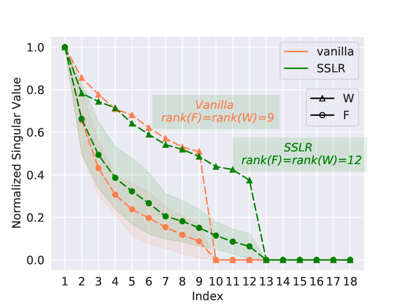
(a) Inlier: Cifar-10 (WideResNet40-2).

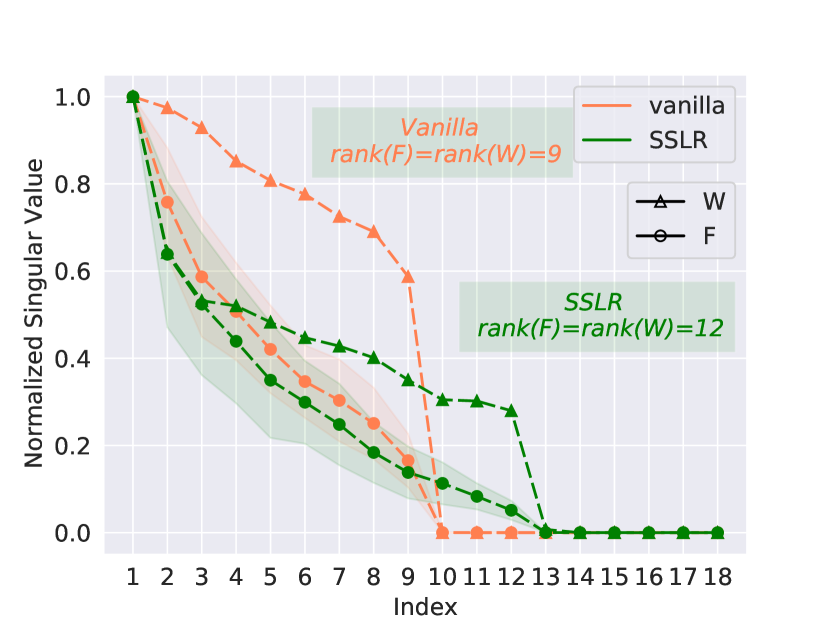
(b) Inlier: SVHN (VGG16).

Figure 1: Normalized singular value of the feature matrix and the classification weight matrix. The normalized singular values decrease to $0$ at exactly the same time for both matrices. Using SSL clearly increases the rank of both the weight and feature matrices.

First of all, in both vanilla and SSLR scenarios, the feature rank and the weight rank exactly matches. The normalized singular values decreases to exactly $0$ at the same time, validating proposition 1 and 2. Secondly, we observe that the rank of feature matrix in the vanilla case is exactly $C-1$ (orange line, $C=10$). This is a reasonable result. The $c$-th output dimension corresponds to the direction $\mathbf{W}_{\cdot c}^{*}$. The loss tries to separate all these directions apart. Given the first $C-1$ directions, the optimal $C$-th direction should be close to the opposite direction of the mean direction of the first $C-1$ directions, making the rank less than $C$. After adding the proxy task, the rank of the features also increases, as the green line shows. The rotation proxy task has $4$ output dimensions, so the rank of the features is $(10-1)+(4-1)=12$.

Feature Dimension in a More Realistic Scenario

The experiments in Section Empirical Validation of the Feature Dimension agree very well with proposition 1 and 2. We also witness that the intrinsic dimension of the overall feature space increases when SSL is added. However, in a more realistic scenario, we directly use the output of the global pooling layer as the feature rather than linearly transform it to another feature space (In the VGG16 case, there will be a nonlinear activation after the fully connected layer in practice). The diagram of the deep network then becomes

$$\bm{x}\xrightarrow{\text{Non-linear}}\bm{f}\xrightarrow{\mathbf{W}}\bm{\eta}\xrightarrow{\textnormal{Softmax}}\bm{\hat{y}}.$$ (6)

In this case, the feature vector $\bm{f}$ only receives gradients in the directions $\{\mathbf{W}_{\cdot c}\}_{c=1}^{C}$. The gradients will propagate back to the nonlinear network to move $\bm{f}$ in the space spanned by $\{\mathbf{W}_{\cdot c}\}_{c=1}^{C}$ such that it can very well align with $\mathbf{W}_{\cdot c}$ of the corresponding class. On the other hand, The component of $\bm{f}$ that is orthogonal to $\{\mathbf{W}_{\cdot c}\}_{c=1}^{C}$ will be eliminated by weight decay. Note that though the weight decay is applied on the weights rather than the feature vectors, it still constraints the length of $\bm{f}$. Since the length of $\bm{f}$ is limited, its component orthogonal to $\{\mathbf{W}_{\cdot c}\}_{c=1}^{C}$ should be as small as possible to minimize the objective. So if the capacity of the network is big enough, $\bm{f}$ will lie in the subspace spanned by $\{\mathbf{W}_{\cdot c}\}_{c=1}^{C}$.

To validate the analysis above, we run the experiments with different network capacity. Again we use the WideResNet architecture but with different widen factors to control the network capacity. Also, we remove the linear transformation layer that is used in Section Empirical Validation of the Feature Dimension. The training scheme is exactly the same as that in Section Empirical Validation of the Feature Dimension. Similarly, we feed both the inliers and the outliers to the optimized network to obtain the features and then calculate the normalized singular values of the feature matrix. The logarithm of the normalized singular values of different widen factors are shown in Figure 2. In this more realistic case, the singular values do not decrease exactly to $0$ at the $10$th dimension in the vanilla case (Figure 2(a)). However, as the network capacity increases, the singular values decrease more sharply near the $10$th dimension, which is consistent with our analysis. When SSL is introduced, the normalized singular values decrease more slowly. They start to decrease very sharply near the $13$th dimension.

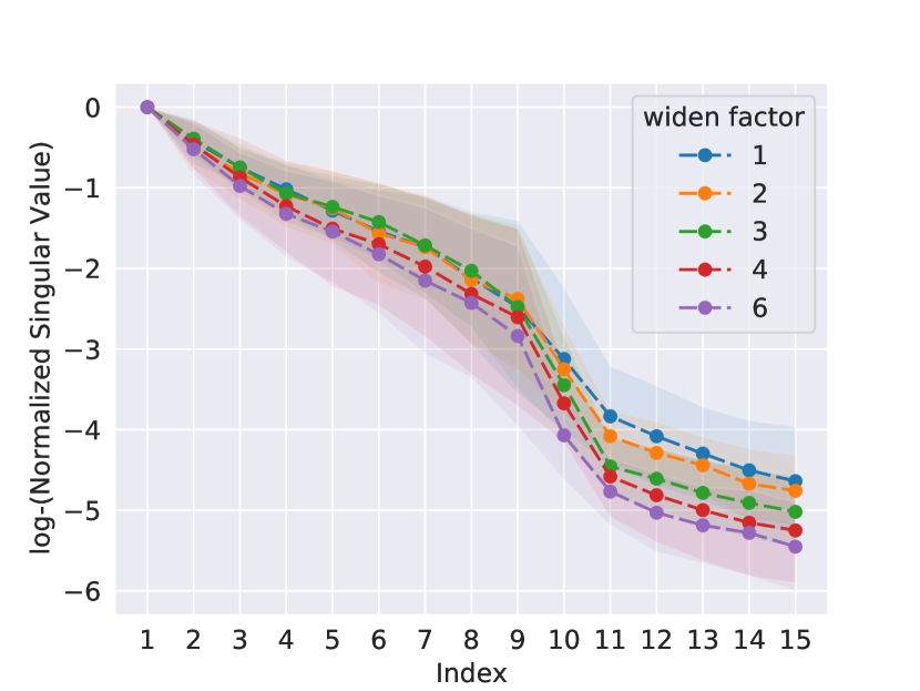
(a) Without SSL.

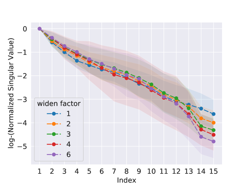
(b) With SSL.

Figure 2: Logarithm of the normalized singular values of the feature matrix with different widen factors. As the widen factor (network capacity) increases, the pattern of the normalized singular values become closer to that in Figure 1.

To better visualize how SSL expands the overall feature dimension, we run a simple experiment on MNIST dataset. Only digit $0$ and $1$ are used as the inliers. The major task is a simple binary classification task. The other $8$ digits are regarded as outliers. For the proxy task, we only use $2$ kinds of transformations: rotation by $0^{\circ}$ and $180^{\circ}$. So the proxy task also becomes a binary classification task. We use the LeNet-5 (LeCun et al. 2015) architecture but reduce the dimension of the feature layer from $84$ to $2$ for visualization convenience. For optimizer, we choose a cosine learning rate schedule with initial learning rate being 0.01 and Nesterov momentum being 0.9. The batch size is $128$ and we train the network for $10$ epochs. The tuning parameter $\lambda$ for rotation auxiliary is $4$. Figure 3 shows the features of both inliers (red) and outliers (green). The dimension of the overall feature space clearly increases from $1$ to $2$ after the SSL head is used.

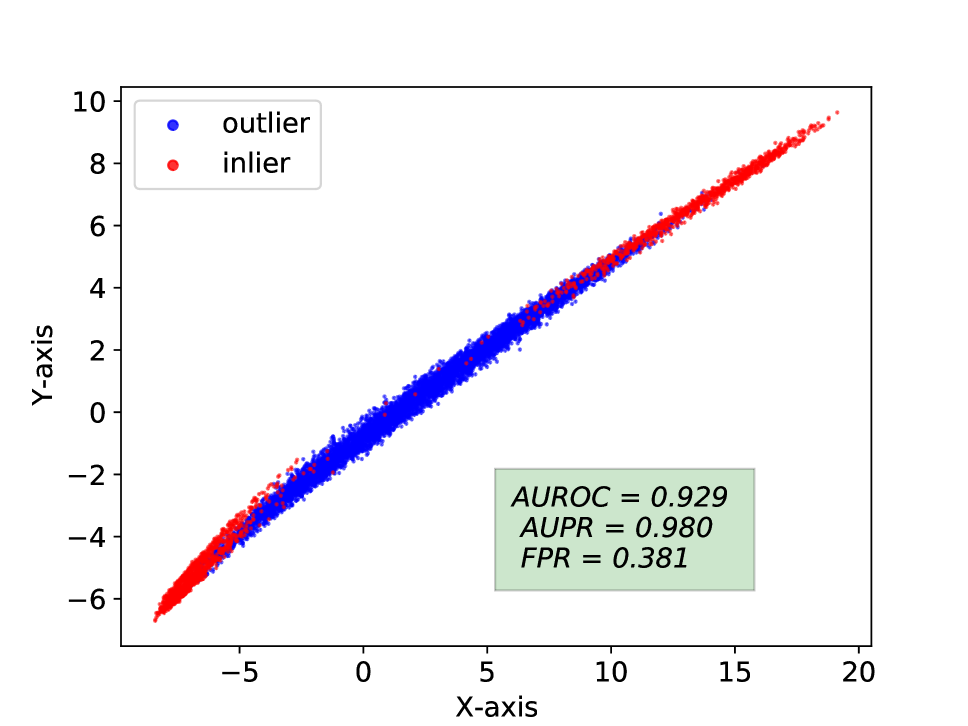
(a) Without SSL.

(b) With SSL.

Figure 3: Feature space without and with SSL. When there is no SSL, the features lie in an approximately $1$-dimensional subspace. Introducing SSL expands the intrinsic dimension of the overall feature space and keeps the intrinsic dimension of each inlier cluster unchanged.

When SSL Can/Cannot Shrink the Inlier Feature Space

We have shown that SSL can expand the overall feature space in Section SSL Expands the Overall Feature Space both theoretically and empirically. However, it does not necessarily mean that SSL can improve the OOD detection performance. SSL can only work when the inlier feature space does not significantly increase. Fortunately this is indeed the case. Moreover, we find that SSL can sometimes even shrink the inlier feature space though the overall feature space is expanded, making the OOD detection even easier.

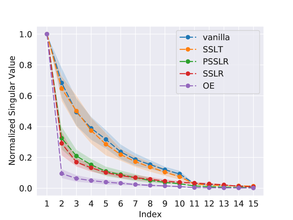
(a) Cifar10 trained on WideResNet40-2

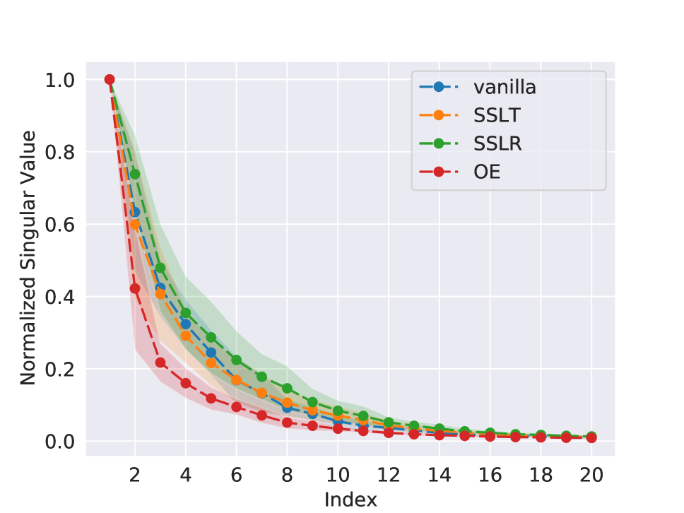
(b) MNIST trained on Lenet5

Figure 4: Mean and standard deviation of the normalized singular values of each inlier class.

We first extract the inlier features of Cifar-10 dataset trained on WideResNet40-2 (corresponding to Figure 2). For each inlier class, we calculate the normalized singular values and sort them in descending order. The mean and standard deviations of the normalized singular values over all the classes are shown in Figure 4(a). It is obvious that the curve of SSLR (red) descends much faster than that of vanilla (blue), indicating that SSL encourages the inliers to use even a smaller feature space.

The reason that SSL shrinks the inlier feature space is that it has a regularization effect. When the network is wide enough, the features in every layer tend to use more dimensions than needed. If the transformed images have different low-level patches, the early convolution layers should leave space for the patches of the transformed images, encouraging the inlier patches to use a smaller space. As a result, the inlier will occupy a smaller feature space in all the layers, including the last feature layer.

This regularization effect can happen even without the SSL loss. We run another experiment with hyper-parameter $\lambda$ being $0$. We call this scheme pseudo SSLR (PSSLR for short). In this case, the transformed images only contributes to updating the running mean and running variance in the batch normalization layers. They do not have any corresponding loss term. Since the running mean and running variance count both the original images and the transformed images, it can also shrink the inlier features in all the layers. The curve is also shown in Figure 4(a) (green line). Surprisingly, the curve is very close to the SSLR case. Its OOD detection performance is also much better than the vanilla scheme (We will show the detailed values later).

Necessary Conditions for SSL to Shrink the Inlier Feature Space

Unfortunately, this regularization effect does not always happen. There are two necessary conditions for it to work: 1) The low-level patches of the transformed images have significantly different statistics than that of the original images; 2) The network capacity is relatively large.

Based on our analysis above, it is obvious that the regularization effect will disappear if the low-level patches of the transformed images are close to those of the original images. To validate this, we run an experiment using SSL with translation transformations (SSLT). In SSLT, the images are vertically or horizontally translated by $-1,0$ or $1$ pixel. The corresponding curve of the normalized singular values (orange curve in Figure 4(a)) descends almost at the same rate as that of the vanilla case.

We then test the OOD detection performance of the models trained using vanilla, SSLT, PSSLR and SSLR schemes on multiple outlier datasets including Cifar-100, SVHN, Texture, LSUN, Place365, Gaussian, Rademacher and Blob. The average performance over all the outlier datasets is shown in Table 1. The vanilla scheme produces the worst performance. The SSLR method, which can simultaneously expand the overall feature space and shrink the inlier feature space is the best among all four methods. SSLT can only expand the overall feature space while PSSLR can only shrink the inlier feature space. Their results are between vanilla and SSLR, which is reasonable.

	AUROC	AUPR	FPR
Vanilla	0.9068	0.8384	0.4376
SSLT	0.9182	0.8404	0.3845
PSSLR	0.9485	0.8827	0.2106
SSLR	0.9652	0.9080	0.1599

Table 1: The performance of outlier detector trained by different methods. Cifar 10 is inlier and all the evaluation metrics are mean value over different outliers (Cifar-100, SVHN, Texture, LSUN, Place365, Gaussian, Rademacher and Blob).

Another necessary condition for SSL to shrink the inlier feature space is that the network capacity should be large enough. If the network is relatively thin, the feature space may be too small to capture all the patterns of the inlier patches. When transformed images with different low-level patches are added in the training phase, both the original image patches and the transformed image patches are entangled in the same low-dimensional space in the early layers, leaving the hard classification problem to future layers. This prohibits the last feature layer using a smaller inlier feature space to achieve good classification performance.

An example is shown in Figure 3, where the network architecture is LeNet5. It only has $6$ channels in the first convolution layer, which is obviously not sufficient to capture all the modes of $5\times 5$ patches. Fortunately, even when the network capacity is sometimes not enough, SSL will not significantly increase the inlier feature space. In Figure 3(b), the inliers still lie in an approximately $1$-dimensional subspace. We further validate this point on the full MNIST dataset using LeNet5 (with the last layer dimension being $84$ rather than $2$). Three different schemes are adopted: vanilla, SSLT and SSLR. The mean and standard deviation of the normalized singular values over all the inlier classes are shown in Figure 4(b). The curve of SSLT decreases at the same rate as that of vanilla, meaning that the inlier feature sizes are very similar in both cases. This is reasonable since they have the same statistics of the low-level patches. In SSLR, where the transformed images become significantly different, the curve is only slightly higher than the vanilla case, indicating that the inlier feature space does not significantly increase.

Connection with Outlier Exposure

Conventional wisdom thinks that SSL serves as a kind of outlier exposure (OE) (Hendrycks, Mazeika, and Dietterich 2019) in OOD detection. Based on our analysis, this is not the whole story. OE will shrink the inlier feature space by explicitly introducing outliers into the training phase. We add a line corresponding to OE in both Figure 4(a) and 4(b). It is obvious that the normalized singular values of OE decreases at the fastest rate. However, there is no mechanism that it can expand the overall feature space. As a result, OE performs no better than SSL though it has even smaller inlier feature space.

Discussion

In this paper, we try to understand the mechanism of SSL in the OOD detection task. We first explicitly pointed out that a good OOD detection model should have large overall feature space and small inlier feature space. Then we demonstrate that SSL can indeed expand the overall feature space both theoretically and empirically. Moreover, SSL can also shrink the inlier feature space under mild conditions. The necessary conditions about when SSL can shrink the inlier feature space is presented and empirically validated. Even when the necessary conditions are violated, SSL is still able to keep the inlier feature space unchanged. The conditions of a good OOD detection model we presented provide us a guideline to design better OOD detectors, which will be our future work.

Though this work only studies the mechanism of SSL in OOD detection task, it can also shed light on other tasks where SSL works. For example, in supervised learning and semi-supervised learning, SSL expands the feature space such that it can disentangle the class information and the rotation (or other transformations) information. In this way, it can avoid a certain kind of overfitting and improve the classification performance. In addition, the regularization mechanism we showed in Section When SSL Can/Cannot Shrink the Inlier Feature Space probably also plays a role in other tasks. Of course the mechanism analyzed in this paper is not the whole story about how SSL works in all the tasks, but we believe this work is a meaningful step towards better understanding the SSL mechanism.

References

- Ackley, Hinton, and Sejnowski (1985) Ackley, D. H.; Hinton, G. E.; and Sejnowski, T. J. 1985. A learning algorithm for Boltzmann machines. Cognitive science, 9(1): 147–169.
- Baevski et al. (2020) Baevski, A.; Zhou, H.; Mohamed, A.; and Auli, M. 2020. wav2vec 2.0: A framework for self-supervised learning of speech representations. arXiv preprint arXiv:2006.11477.
- Caron et al. (2020) Caron, M.; Misra, I.; Mairal, J.; Goyal, P.; Bojanowski, P.; and Joulin, A. 2020. Unsupervised learning of visual features by contrasting cluster assignments. arXiv preprint arXiv:2006.09882.
- Chalapathy, Menon, and Chawla (2018) Chalapathy, R.; Menon, A. K.; and Chawla, S. 2018. Anomaly detection using one-class neural networks. arXiv preprint arXiv:1802.06360.
- Chen et al. (2020a) Chen, T.; Kornblith, S.; Norouzi, M.; and Hinton, G. 2020a. A simple framework for contrastive learning of visual representations. arXiv preprint arXiv:2002.05709.
- Chen et al. (2020b) Chen, X.; Fan, H.; Girshick, R.; and He, K. 2020b. Improved baselines with momentum contrastive learning. arXiv preprint arXiv:2003.04297.
- Cimpoi et al. (2014) Cimpoi, M.; Maji, S.; Kokkinos, I.; Mohamed, S.; ; and Vedaldi, A. 2014. Describing Textures in the Wild. In Proceedings of the IEEE Conf. on Computer Vision and Pattern Recognition (CVPR).
- Davis and Goadrich (2006) Davis, J.; and Goadrich, M. 2006. The relationship between Precision-Recall and ROC curves. In Proceedings of the 23rd international conference on Machine learning, 233–240.
- Doersch, Gupta, and Efros (2015) Doersch, C.; Gupta, A.; and Efros, A. A. 2015. Unsupervised visual representation learning by context prediction. In Proceedings of the IEEE international conference on computer vision, 1422–1430.
- Dosovitskiy et al. (2015) Dosovitskiy, A.; Fischer, P.; Springenberg, J. T.; Riedmiller, M.; and Brox, T. 2015. Discriminative unsupervised feature learning with exemplar convolutional neural networks. IEEE transactions on pattern analysis and machine intelligence, 38(9): 1734–1747.
- Gidaris, Singh, and Komodakis (2018) Gidaris, S.; Singh, P.; and Komodakis, N. 2018. Unsupervised representation learning by predicting image rotations. arXiv preprint arXiv:1803.07728.
- He et al. (2020) He, K.; Fan, H.; Wu, Y.; Xie, S.; and Girshick, R. 2020. Momentum contrast for unsupervised visual representation learning. In Proceedings of the IEEE/CVF Conference on Computer Vision and Pattern Recognition, 9729–9738.
- Hendrycks and Gimpel (2016) Hendrycks, D.; and Gimpel, K. 2016. A baseline for detecting misclassified and out-of-distribution examples in neural networks. arXiv preprint arXiv:1610.02136.
- Hendrycks, Mazeika, and Dietterich (2019) Hendrycks, D.; Mazeika, M.; and Dietterich, T. 2019. Deep Anomaly Detection with Outlier Exposure. arXiv:1812.04606.
- Hendrycks et al. (2019) Hendrycks, D.; Mazeika, M.; Kadavath, S.; and Song, D. 2019. Using Self-Supervised Learning Can Improve Model Robustness and Uncertainty. In Advances in Neural Information Processing Systems, 15663–15674.
- Kolesnikov, Zhai, and Beyer (2019) Kolesnikov, A.; Zhai, X.; and Beyer, L. 2019. Revisiting self-supervised visual representation learning. In Proceedings of the IEEE conference on Computer Vision and Pattern Recognition, 1920–1929.
- Krizhevsky, Hinton et al. (2009) Krizhevsky, A.; Hinton, G.; et al. 2009. Learning multiple layers of features from tiny images.
- Lan et al. (2019) Lan, Z.; Chen, M.; Goodman, S.; Gimpel, K.; Sharma, P.; and Soricut, R. 2019. Albert: A lite bert for self-supervised learning of language representations. arXiv preprint arXiv:1909.11942.
- Larsson, Maire, and Shakhnarovich (2016) Larsson, G.; Maire, M.; and Shakhnarovich, G. 2016. Learning representations for automatic colorization. In European conference on computer vision, 577–593. Springer.
- LeCun et al. (2015) LeCun, Y.; et al. 2015. LeNet-5, convolutional neural networks. URL: http://yann. lecun. com/exdb/lenet, 20(5): 14.
- Lee, Hwang, and Shin (2019) Lee, H.; Hwang, S. J.; and Shin, J. 2019. Rethinking data augmentation: Self-supervision and self-distillation. arXiv preprint arXiv:1910.05872.
- Lee et al. (2018) Lee, K.; Lee, K.; Lee, H.; and Shin, J. 2018. A simple unified framework for detecting out-of-distribution samples and adversarial attacks. In Advances in Neural Information Processing Systems, 7167–7177.
- Liang, Li, and Srikant (2017) Liang, S.; Li, Y.; and Srikant, R. 2017. Enhancing the reliability of out-of-distribution image detection in neural networks. arXiv preprint arXiv:1706.02690.
- Manning and Schutze (1999) Manning, C.; and Schutze, H. 1999. Foundations of statistical natural language processing. MIT press.
- Mikolov et al. (2013) Mikolov, T.; Chen, K.; Corrado, G.; and Dean, J. 2013. Efficient estimation of word representations in vector space. arXiv preprint arXiv:1301.3781.
- Netzer et al. (2011) Netzer, Y.; Wang, T.; Coates, A.; Bissacco, A.; Wu, B.; and Ng, A. Y. 2011. Reading digits in natural images with unsupervised feature learning.
- Noroozi and Favaro (2016) Noroozi, M.; and Favaro, P. 2016. Unsupervised learning of visual representations by solving jigsaw puzzles. In European Conference on Computer Vision, 69–84. Springer.
- Oord, Li, and Vinyals (2018) Oord, A. v. d.; Li, Y.; and Vinyals, O. 2018. Representation learning with contrastive predictive coding. arXiv preprint arXiv:1807.03748.
- Sehwag, Chiang, and Mittal (2021) Sehwag, V.; Chiang, M.; and Mittal, P. 2021. {SSD}: A Unified Framework for Self-Supervised Outlier Detection. In International Conference on Learning Representations.
- Simonyan and Zisserman (2014) Simonyan, K.; and Zisserman, A. 2014. Very deep convolutional networks for large-scale image recognition. arXiv preprint arXiv:1409.1556.
- Srinivas, Laskin, and Abbeel (2020) Srinivas, A.; Laskin, M.; and Abbeel, P. 2020. Curl: Contrastive unsupervised representations for reinforcement learning. arXiv preprint arXiv:2004.04136.
- Sutskever et al. (2013) Sutskever, I.; Martens, J.; Dahl, G.; and Hinton, G. 2013. On the importance of initialization and momentum in deep learning. In International conference on machine learning, 1139–1147.
- Tack et al. (2020) Tack, J.; Mo, S.; Jeong, J.; and Shin, J. 2020. Csi: Novelty detection via contrastive learning on distributionally shifted instances. Advances in Neural Information Processing Systems, 33.
- Tian et al. (2021) Tian, Y.; Yu, L.; Chen, X.; and Ganguli, S. 2021. Understanding Self-supervised Learning with Dual Deep Networks.
- Tran (2019) Tran, P. V. 2019. Exploring Self-Supervised Regularization for Supervised and Semi-Supervised Learning. arXiv preprint arXiv:1906.10343.
- Wang and Isola (2020) Wang, T.; and Isola, P. 2020. Understanding Contrastive Representation Learning through Alignment and Uniformity on the Hypersphere. arXiv preprint arXiv:2005.10242.
- Zagoruyko and Komodakis (2016) Zagoruyko, S.; and Komodakis, N. 2016. Wide residual networks. arXiv preprint arXiv:1605.07146.
- Zhou et al. (2017) Zhou, B.; Lapedriza, A.; Khosla, A.; Oliva, A.; and Torralba, A. 2017. Places: A 10 million Image Database for Scene Recognition. IEEE Transactions on Pattern Analysis and Machine Intelligence.