Complete classification of Friedmann-Lemaître-Robertson-Walker solutions with linear equation of state: parallelly propagated curvature singularities for general geodesics

Abstract

We completely classify the Friedmann-Lemaître-Robertson-Walker solutions with spatial curvature $K=0,\pm 1$ for perfect fluids with linear equation of state $p=w\rho$, where $\rho$ and $p$ are the energy density and pressure, without assuming any energy conditions. We extend our previous work to include all geodesics and parallelly propagated curvature singularities, showing that no non-null geodesic emanates from or terminates at the null portion of conformal infinity and that the initial singularity for $K=0,-1$ and $-5/3<w<-1$ is a null non-scalar polynomial curvature singularity. We thus obtain the Penrose diagrams for all possible cases and identify $w=-5/3$ as a critical value for both the future big-rip singularity and the past null conformal boundary.

I Introduction and summary

The Friedmann-Lemaître-Robertson-Walker (FLRW) spacetime is unique as a spatially homogeneous and isotropic spacetime [1]. Its metric has spatial curvature $K=0,\pm 1$ and it is generally accepted that this, together with the Einstein equation, approximately describes our Universe. For the matter content, a perfect fluid with linear equation of state $p=w\rho$ is often adopted, where $\rho$ and $p$ are the energy density and pressure, respectively, and $w$ is a constant. Recent observations strongly suggest the acceleration of the cosmological expansion. This implies the existence of dark energy with equation of state parameter $w<-1/3$. Cosmological observations require $w=-1.00^{+0.04}_{-0.05}$ [2] and restrict the spatial curvature to $\Omega_{K}=0.000\pm 0.005$ [3].

Linear equations of state with $w=1/3$, $0$ and $-1$ correspond to a Universe dominated by radiation, dust and a cosmological constant, respectively. Phenomenologically, $w=1$, $-1/3$ and $-2/3$ correspond to a massless scalar field (or stiff fluid), a string network and a domain wall network, respectively. The ranges $-1/3<w<-1$ and $w<-1$ correspond to quintessence [4, 5] and a phantom field [6], respectively. The null energy condition corresponds to $(1+w)\rho\geq 0$ but viable modified theories of gravity may violate this [7]. The FLRW spacetime not only provides a realistic model for the whole Universe; it may also represent part of the Universe. The most famous example is the Oppenheimer-Snyder solution [8], where the FLRW solution describes the metric inside a uniform ball which is collapsing to a black hole. FLRW spacetimes can also be used to model the formation of a primordial black hole [9, 10] and a stable gravastar [11, 12].

The conformal structure and singularities are the basic properties of any spacetime. The Penrose diagrams for the flat FLRW solutions are summarised in reference [13] for models satisfying the dominant energy condition ($\rho\geq 0$ and $-1\leq w\leq 1$). The possibility of big-rip singularities has been proposed for $w<-1$ in references [14, 15, 16] and the behaviour of geodesics around the big-bang, big-crunch and big-rip singularities has been analysed in detail in reference [17]. More exotic types of FLRW singularities, such as weak ones, are investigated in reference [18]. Recently, the past extendibility of inflationary FLRW Universes has been discussed in references [19, 20].

In reference [21], which we will refer to as Paper I, all of the FLRW solutions with $p=w\rho$ are given without assuming any energy conditions and the corresponding Penrose diagrams are drawn, analysing null and comoving timelike geodesics, scalar polynomial (s.p.) curvature singularities, trapped regions and trapping horizons. This paper extends that analysis to include all geodesics and parallelly propagated (p.p.) curvature singularities. This enables us to study the physical properties of singularities, such as the fate of free-falling observers, in complete generality. We conclude that the null portion of conformal infinity repels non-null geodesics in the Penrose diagram, so that no non-null geodesic can emanate from or terminate at the null portion of conformal infinity. By introducing p.p. curvature singularities, which do not necessarily involve the divergence of any fluid quantities, we can study the extendibility of the spacetime beyond the conformal boundaries with $C^{2-}$ metrics. We conclude that the flat and negative-curvature solutions are past inextendible beyond the null boundary for $-5/3<w<-1$, which means that these cases also have an initial singularity problem.

Before proceeding to technicalities, we summarise our main results. The conformal structure of the FLRW solutions depends on the signs of $K$ and $\rho$; it also depends on $w$, together with an integration constant in the special case $w=-1/3$. The Penrose diagrams for the flat case with $\rho=0$ (Minkowski spacetime) and $\rho>0$ are shown in figures 1 and 2, respectively. The black solid, black dotted, black dashed-double-dotted, blue dashed-dotted and red dashed lines denote regular centres, extendible conformal boundaries, line-like conformal infinities, non-s.p. curvature singularities and s.p. curvature singularities, respectively, and the black filled, black open and red open circles denote point-like extendible boundaries, infinities and s.p. curvature singularities, respectively. The past null boundary for the flat case is a non-s.p. curvature singularity for $-5/3<w<-1$. The Penrose diagrams for the positive-curvature case are shown in figure 3. Those for the negative-curvature case with $\rho=0$ (Milne spacetime), $\rho>0$ and $\rho<0$ are shown in figures 4, 5 and 6, respectively. For the negative-curvature case with $-5/3<w<-1$, the past null boundary with $\rho>0$ is a non-s.p. curvature singularity; this also applies for the future and past null boundaries with $\rho<0$.

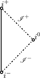
Figure 1: The Penrose diagram for Minkowski spacetime, included for completeness.

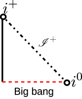
(a) $w>-1/3$ (F1)

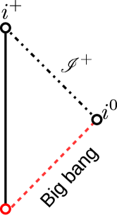
(b) $w=-1/3$ (F2)

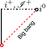
(c) $-1<w<-1/3$ (F3)

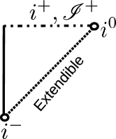
(d) $w=-1$ (dS)

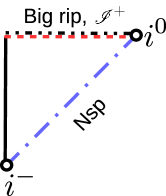
(e) $-5/3<w<-1$ (F4a)

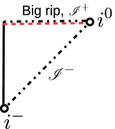
(f) $w=-5/3$ (F4b)

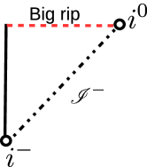
(g) $w<-5/3$ (F4c)

Figure 2: The Penrose diagrams for flat FLRW solutions with the positive density.

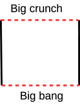
(a) $w>-1/3$ (P1)

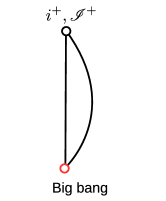
(b) $w=-1/3$ (P2a)

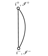
(c) $w=-1/3$ (P2b)

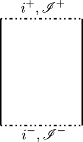
(d) $-1<w<-1/3$ (P3)

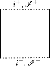
(e) $w=-1$ (dS)

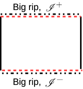
(f) $-5/3\leq w<-1$ (P4a)

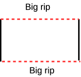
(g) $w<-5/3$ (P4b)

Figure 3: The Penrose diagrams for positive-curvature FLRW solutions.

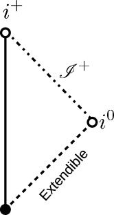
Figure 4: The Penrose diagram for Milne spacetime.

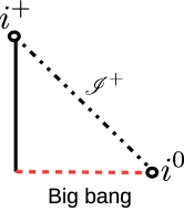
(a) $w>-1/3$ (NP1)

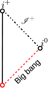
(b) $w=-1/3$ (NP2)

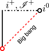
(c) $-1<w<-1/3$ (NP3)

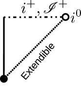
(d) $w=-1$ (dS)

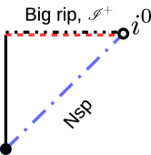
(e) $-5/3<w<-1$ (NP4a)

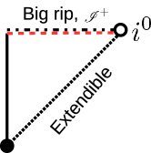
(f) $w=-5/3$ (NP4b)

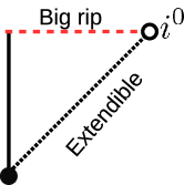
(g) $w<-5/3$ (NP4c)

Figure 5: The Penrose diagrams for negative-curvature FLRW solutions with the positive density.

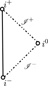
(a) $w>-1/3$ (NN1)

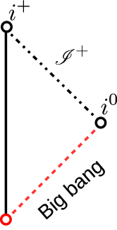
(b) $w=-1/3$ (NN2a)

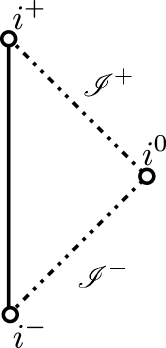
(c) $w=-1/3$ (NN2b)

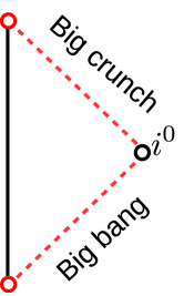
(d) $-1<w<-1/3$ (NN3)

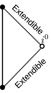
(e) $w=-1$ (AdS)

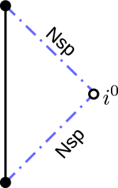
(f) $-5/3<w<-1$ (NN4a)

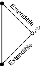
(g) $w\leq-5/3$ (NN4b)

Figure 6: The Penrose diagrams for negative-curvature FLRW solutions with the negative density.

The Penrose diagrams for the flat FLRW solutions with $-1<w<1$, investigated in reference [13], have a big-bang spacelike singularity for $-1/3<w<1$ and a big-bang null singularity for $-1<w<-1/3$ at the past boundary; they also have a future null infinity at the future boundary. For $w\leq-1/3$, there is unexpectedly rich structure with a variety of past and future boundaries. For $\rho>0$ and $w<-1$, the spacetime commonly ends with a future big-rip spacelike singularity, although for $-5/3\leq w<-1$, it is still future null geodesically complete. This is consistent with reference [17]. In the flat and negative-curvature cases with $\rho>0$, the expanding Universe begins with a big-bang spacelike singularity for $w>-1/3$, a big-bang null singularity for $-1<w\leq-1/3$ and a non-s.p. curvature null singularity for $-5/3<w<-1$. This implies that no quasi-exponential inflationary model avoids the initial singularity problem if it is described by the flat or negative-curvature solutions with $-5/3<w<-1$ or $-1<w<-1/3$. For $w\leq-5/3$, the flat and negative-curvature solutions have a past null infinity and a past extendible null boundary, respectively. For $K=1$ and $w<-1/3$, the solution describes a bouncing Universe, which is singularity-free for $-1\leq w<-1/3$ but has past and future big-rip singularities for $w<-1$. For $w>-5/3$ and $\rho>0$, no spacelike geodesic emanates from or terminates at the spacelike infinity in the flat and negative-curvature cases. Although the nature of the matter corresponding to $w=-5/3$ is unclear, the Einstein equation suggests that this value is just as critical as $1/3$, $-1/3$ and $-1$.

The paper is organised as follows. Section II gives the conformal completion of the FLRW spacetimes and the corresponding solutions of the Einstein equation for $p=w\rho$. Section III derives expressions for general geodesics and the Ricci tensor components in the p.p. frame. Section IV provides the definition of singularities and infinities as conformal boundaries. We analyse the conformal boundaries of the FLRW solutions and infer the Penrose diagrams. Appendix A gives a list of abbreviations and Appendix B gives some important integrals. Henceforth we use units with $c=G=1$ and the abstract index notation in Wald’s textbook [1].

II The FLRW spacetime

II.1 Conformal completion

The line element in the FLRW spacetime is written in the following form:

$$ds^{2} = -dt^{2}+a^{2}(t)[dr^{2}+\Sigma_{K}^{2}(r)d\Omega^{2}]$$ (1)

$$= a^{2}(\eta)[-d\eta^{2}+dr^{2}+\Sigma_{K}^{2}(r)d\Omega^{2}],$$

where $a>0$, $ad\eta=dt$, $d\Omega^{2}=d\theta^{2}+\sin^{2}\theta d\phi^{2}$ with $0\leq\theta\leq\pi$ and $0\leq\phi<2\pi$, and

$$\Sigma_{K}(r)=\left\{\begin{array}[]{cc}r&(K=0)\\ \sin r&(K=1)\\ \sinh r&(K=-1)\end{array}\right..$$ (5)

The domain of the coordinates $(r,\eta)$ depends on the spatial curvature and is given by

$$-\infty<\eta<\infty,~{}\left\{\begin{array}[]{cc}0\leq r<\infty{}&(K=0,-1)\\ 0\leq r\leq\pi&(K=1)\\ \end{array}\right.$$ (6)

unless $\eta$ is restricted to a smaller interval by the specific solution.

The conformal completion prescribes the “boundary” of the spacetime $M$. If this is conformally isometric to a bounded open region of the “unphysical” spacetime $\tilde{M}$, the boundary of the image of $M$ in $\tilde{M}$ is called the conformal boundary [22, 1]. The line element in the flat FLRW spacetime can be rewritten as

$$ds^{2}=\frac{1}{4}a^{2}(\eta)\sec^{2}\left(\frac{\tau+\chi}{2}\right)\sec^{2}\left(\frac{\tau-\chi}{2}\right)(-d\tau^{2}+d\chi^{2}+\sin^{2}\chi d\Omega^{2}),$$ (7)

where

$$\tau=\arctan(\eta+r)+\arctan(\eta-r),\quad\chi=\arctan(\eta+r)-\arctan(\eta-r).$$ (8)

Thus, the physical spacetime is conformally isometric to the bounded region $\chi\geq 0$, $\tau-\chi>-\pi$ and $\tau+\chi<\pi$ in the Einstein static Universe. The domain of $(\chi,\tau)$ is the isosceles right-angled triangle in figure 7(a). We denote the top and bottom vertices, the apex and the midpoint of the base by N, S, E and O, respectively. The coordinates $(\chi,\tau)$ of N, S, E and O are $(0,\pi)$, $(0,-\pi)$, $(\pi,0)$ and $(0,0)$, respectively.

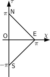
(a)

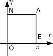
(b)

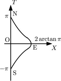
(c)

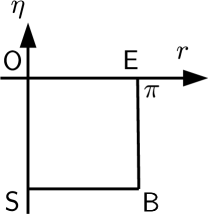
(d)

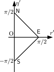
(e)

Figure 7: The domain of the coordinate planes for (a) the flat case, the positive-curvature cases for (b) $w>-1/3$, (c) $w=-1/3$ and (d) $w<-1/3$, and (e) the negative-curvature case.

For the positive-curvature case, the line element is already conformal to that of the Einstein static Universe. As we will see in Sec. II.2, the domain of $\eta$ depends on the parameter $w$. For $w>-1/3$ and $w<-1/3$, the domains are restricted to the bounded intervals $0<\eta<2\pi/(1+3w)$ and $2\pi/(1+3w)<\eta<0$, respectively. Since the domain of $r$ is also bounded, the domains of $(r,\eta)$ for $w>-1/3$ and $w<-1/3$ are both given by rectangles, as depicted in figures 7(b) and 7(d), respectively, so no conformal rescaling is needed. For $w>-1/3$, we denote the top left, top right, bottom left and bottom right vertices by N, A, O and E, respectively, and their coordinates $(r,\eta)$ are $(0,2\pi/(1+3w))$, $(\pi,2\pi/(1+3w))$, $(0,0)$ and $(\pi,0)$, respectively. For $w<-1/3$, we denote the top left, top right, bottom left and bottom right vertices by O, E, S and B, respectively, with coordinates $(0,0)$, $(\pi,0)$, $(0,2\pi/(1+3w))$ and $(\pi,2\pi/(1+3w))$, respectively. However, in the exceptional case $w=-1/3$, the domain of $\eta$ is unbounded ($-\infty<\eta<\infty$) and we can use the line element

$$ds^{2} = \frac{1}{4}a^{2}(\eta)\sec^{2}\frac{T+X}{2}\sec^{2}\frac{T-X}{2}$$ (9)

$$\times \left(-dT^{2}+dX^{2}+4\cos^{2}\frac{T+X}{2}\cos^{2}\frac{T-X}{2}\sin^{2}rd\Omega^{2}\right),$$

where

$$T=\arctan(\eta+r)+\arctan(\eta-r),\quad X=\arctan(\eta+r)-\arctan(\eta-r).$$ (10)

Thus, the physical spacetime is conformally isometric to the bounded region

$$X\geq 0,-\pi<T<\pi,~{}\tan\frac{T+X}{2}-\tan\frac{T-X}{2}\leq 2\pi\,,$$ (11)

as depicted in figure 7(c). Here we denote the top, bottom and right vertices by N, S and E, respectively, and the midpoint of the line segment $\overline{\sf NS}$ by O. The coordinates $(X,T)$ of N, S, E and O are $(0,\pi)$, $(0,-\pi)$, $(2\arctan\pi,0)$ and $(0,0)$, respectively.

For the negative-curvature case, the line element can be rewritten as

$$ds^{2}=\frac{a^{2}(\eta)}{\cos(r^{\prime}+\eta^{\prime})\cos(r^{\prime}-\eta^{\prime})}(-d\eta^{\prime 2}+dr^{\prime 2}+\sin^{2}r^{\prime}d\Omega^{2}),$$ (12)

where

$$\tan\eta^{\prime}=\frac{\sinh\eta}{\cosh r},\quad\tan r^{\prime}=\frac{\sinh r}{\cosh\eta}~{}.$$ (13)

The original domain is mapped to the isosceles right-angled triangle

$$r^{\prime}\geq 0,\quad\eta^{\prime}-r^{\prime}>-\frac{\pi}{2},\quad\eta^{\prime}+r^{\prime}<\frac{\pi}{2}.$$ (14)

Thus, the physical spacetime is conformally isometric to a bounded region in the Einstein static Universe as depicted in figure 7(e), where we donote the top and bottom vertices, the apex and the midpoint of the base by N, S, E and O, respectively, and the coordinates $(r^{\prime},\eta^{\prime})$ of N, S, E and O are $(0,\pi/2)$, $(0,-\pi/2)$, $(\pi/2,0)$ and $(0,0)$, respectively.

II.2 FLRW solutions with $p=w\rho$

The Einstein equation implies that the matter field must have the perfect-fluid form

$$T^{ab}=(\rho+p)u^{a}u^{b}+pg^{ab},$$ (15)

where $\rho$, $p$ and $u^{a}:=a^{-1}(\partial/\partial\eta)^{a}$ are the energy density, pressure and four-velocity of the fluid element, respectively. If we further assume $p=w\rho$ with $w=\mathrm{const}$, the conservation law $\nabla^{a}T_{ab}=0$ implies

$$\rho=\rho_{0}\left(\frac{a_{0}}{a}\right)^{3(1+w)},$$ (16)

where $\rho=\rho_{0}$ when $a=a_{0}$. For $w\neq-1/3$, the Einstein equation reduces to

$$\left(\frac{d\tilde{a}}{d\tilde{t}}\right)^{2}=\frac{\tilde{a}_{c}}{\tilde{a}}-K,$$ (17)

where

$$\tilde{a}:=a^{1+3w},~{}~{}d\tilde{t}:=(1+3w)\tilde{a}^{3w/(1+3w)}dt,~{}~{}\tilde{a}_{c}:=\frac{8\pi}{3}\rho_{0}a_{0}^{3(1+w)}.$$ (18)

For $w=-1/3$, it becomes

$$\left(\frac{da}{dt}\right)^{2}=\tilde{a}_{c}-K,$$ (19)

where

$$\tilde{a}_{c}:=\frac{8\pi}{3}\rho_{0}a_{0}^{2}.$$ (20)

For the vacuum case, only $K=0$ and $K=-1$ are possible. For $K=0$, the solution is $a=a_{0}=\mathrm{const}$, corresponding to Minkowski spacetime, while for $K=-1$, it is $a=b_{0}e^{\eta}$ with $b_{0}$ being a positive constant, corresponding to Milne spacetime. The domain of $\eta$ is $-\infty<\eta<\infty$ for both of the cases.

For the non-vacuum case, we first consider $w\neq-1/3$. For $K=0$ and $\rho>0$, equation (17) can be integrated to give

$$a(\eta)=\begin{cases}b_{0}\eta^{\alpha}&\quad\mbox{for}~{}~{}0<\eta<\infty~{}~{}(w>-1/3)\\ b_{0}(-\eta)^{\alpha}&\quad\mbox{for}~{}~{}-\infty<\eta<0~{}~{}(w<-1/3)\end{cases},$$ (21)

where $\alpha:=2/(1+3w)$, $b_{0}$ is a positive constant and only an expanding branch is focused. This class contains the Einstein-de Sitter Universe ($w=0$) and de Sitter spacetime in the flat chart ($w=-1$). For $K=1$, the energy density must be positive and equation (17) can be integrated to give

$$\tilde{a}=\tilde{a}_{c}\frac{1-\cos\tilde{\eta}}{2}\,,\quad\tilde{t}=\tilde{a}_{c}\frac{\tilde{\eta}-\sin\tilde{\eta}}{2}$$ (22)

with $\eta=\tilde{\eta}/(1+3w)$, which contains de Sitter spacetime in the global chart ($w=-1$). The domain of $\eta$ is thus $0<\eta<2\pi/(1+3w)$ and $2\pi/(1+3w)<\eta<0$ for $w>-1/3$ and $w<-1/3$, respectively. For $K=-1$ and $\rho>0$, equation (17) can be integrated to give

$$\tilde{a}=\tilde{a}_{c}\frac{\cosh\tilde{\eta}-1}{2}\,,~{}\tilde{t}=\tilde{a}_{c}\frac{\sinh\tilde{\eta}-\tilde{\eta}}{2}\,,$$ (23)

which contains de Sitter spacetime in the open chart ($w=-1$). The domain of $\eta$ is $0<\eta<\infty$ and $-\infty<\eta<0$ for $w>-1/3$ and $w<-1/3$, respectively. For $K=-1$ and $\rho<0$,

$$\tilde{a}=\tilde{a}^{\prime}_{c}\frac{1+\cosh\tilde{\eta}}{2},~{}~{}\tilde{t}=\tilde{a}^{\prime}_{c}\frac{\tilde{\eta}+\sinh\tilde{\eta}}{2}\,$$ (24)

with $\tilde{a}_{c}^{\prime}=-\tilde{a}_{c}$, which contains anti-de Sitter spacetime in the open chart ($w=-1$). The domain of $\eta$ is $-\infty<\eta<\infty$.

For the $w=-1/3$ non-vacuum case, equation (19) again implies that the energy density can be negative only for $K=-1$. For $\tilde{a}_{c}-K>0$, equation (19) can be integrated to give $a=b_{0}e^{b_{c}\eta},$ with $b_{0}$ being a positive constant and $b_{c}=\sqrt{\tilde{a}_{c}-K}$, while for $\tilde{a}_{c}-K=0$, the solution is static and $a=a_{0}=\mbox{const}.$ The domain of $\eta$ is $-\infty<\eta<\infty$ for both of the cases.

III Geodesics, spacelike curves and the Riemann tensor

III.1 Geodesics and spacelike curves

Due to the symmetry, without loss of generality we can consider geodesics in the two-dimensional timelike plane $\theta=\pi/2$ and $\phi=0$. The Lagrangian then takes the simplified form

$$L=\frac{1}{2}a^{2}(\eta)(-\dot{\eta}^{2}+\dot{r}^{2}),$$ (25)

where the dot denotes differentiation with respect to the affine parameter $\lambda$. The Euler-Lagrange equations are

$$\frac{d}{d\lambda}(a^{2}\dot{\eta})+aa^{\prime}(-\dot{\eta}^{2}+\dot{r}^{2}) = 0,$$ (26)

$$\frac{d}{d\lambda}(a^{2}\dot{r}) = 0,$$ (27)

where the prime denotes differentiation with respect to $\eta$. The above equations can be integrated to give

$$\dot{r} = \frac{C}{a^{2}},$$ (28)

$$a^{2}(-\dot{\eta}^{2}+\dot{r}^{2}) = D\,,$$ (29)

where $C$ and $D$ are constants. We can rescale $\lambda$ so that $D=1$ and $-1$ for the spacelike and timelike geodesics, respectively, while $D=0$ for the null geodesics. Clearly, $r$ has no turning point.

If we take $\eta=\eta(\lambda)$, equations (28) and (29) reduce to the one-dimensional potential form

$$\dot{\eta}^{2}+V_{\eta}(\eta)=0\quad{\rm with}\quad V_{\eta}(\eta)=-\frac{C^{2}}{a^{4}(\eta)}+\frac{D}{a^{2}(\eta)}.$$ (30)

This implies that $\eta$ has no turning point for $D=0,-1$, while the allowed region is given by $a(\eta)\leq|C|$ for $D=1$ with a turning point at $\eta=\eta_{\rm tp}$ where $a(\eta_{\rm tp})=|C|$. As $r=0$ is a regular centre, $C$ becomes $-C$ as the geodesic passes through there. We classify geodesics as follows.

• Null geodesic ($D=0$). If we take the affine parameter to have $\dot{\eta}>0$, equation (29) can be integrated to give

  $$\eta-\eta_{0}=\pm(r-r_{0}),$$ (31)

  where $\eta=\eta_{0}$ when $r=r_{0}$. We can make $C=\pm 1$ by rescaling $\lambda$, so that

  $$\lambda-\lambda_{0}=\int^{\eta}_{\eta_{0}}a^{2}(\tilde{\eta})d\tilde{\eta},$$ (32)

  where $\lambda=\lambda_{0}$ when $\eta=\eta_{0}$.

• Timelike geodesic ($D=-1$). We again take $\dot{\eta}>0$, giving two cases.

  • Comoving timelike geodesic (CTG) ($C=0$): Equations (28) and (29) can be integrated to give

    $$\lambda-\lambda_{0}=\int^{\eta}_{\eta_{0}}a(\tilde{\eta})d\tilde{\eta}=t-t_{0},\quad r=r_{0}.$$ (33)

    An observer on this world line sees the Universe isotropic.

  • Non-comoving timelike geodesic (NCTG) $(C\neq 0)$. Equations (28) and (29) can be integrated to give

    $$\lambda-\lambda_{0} = \int^{\eta}_{\eta_{0}}\frac{a(\tilde{\eta})d\tilde{\eta}}{\sqrt{1+(C/a(\tilde{\eta}))^{2}}}\,,$$ (34)

    $$r-r_{0} = \int^{\eta}_{\eta_{0}}\frac{Cd\tilde{\eta}}{\sqrt{a^{2}(\tilde{\eta})+C^{2}}}\,.$$ (35)

    The latter can be transformed to

    $$(\eta-\eta_{0})-\sigma(r-r_{0})=\int^{\eta}_{\eta_{0}}\left(1-\frac{1}{\sqrt{1+(a(\tilde{\eta})/C)^{2}}}\right)d\tilde{\eta}\,,\\$$ (36)

    where $\sigma:=\mathrm{sgn}(dr/d\eta)$.

• Spacelike geodesic ($D=1$). Equation (30) implies $C\neq 0$, so $a(\eta)$ cannot be greater than $|C|$ along spacelike geodesics. This gives two cases.

  • Instantaneous spacelike geodesic (ISG). If we assume $\eta=\eta_{0}=\mbox{const}$, equations (26) and (30) imply $a^{\prime}(\eta_{0})=0$ and $C=\pm a(\eta_{0})$. Equation (28) can then be integrated to give $\lambda-\lambda_{0}=C(r-r_{0})$. This geodesic is an orbit of a Killing vector of spatial translation in the isometry group associated with the homogeneity of the spacelike hypersurface.

  • Non-instantaneous spacelike geodesic (NISG). The geodesic equations can be integrated to give

    $$\lambda-\lambda_{0} = \sigma_{\eta}\int^{\eta}_{\eta_{0}}\frac{a(\tilde{\eta})d\tilde{\eta}}{\sqrt{(C/a(\tilde{\eta}))^{2}-1}},$$ (37)

    $$r-r_{0} = \sigma_{\eta}\int^{\eta}_{\eta_{0}}\frac{C}{\sqrt{C^{2}-a^{2}(\tilde{\eta})}}d\tilde{\eta},$$ (38)

    where $\sigma_{\eta}:=\mathrm{sgn}(\dot{\eta})$. The latter equation can be transformed to

    $$(\eta-\eta_{0})-\sigma(r-r_{0})=-\int_{\eta_{0}}^{\eta}\left(\frac{1}{\sqrt{1-(a(\tilde{\eta})/C)^{2}}}-1\right)d\tilde{\eta},$$ (39)

    where $\sigma=\mathrm{sgn}(dr/d\eta)$.

• Instantaneous spacelike curve (ISC). We consider a spacelike curve given by $\eta=\eta_{0}$. This is not a geodesic unless $a^{\prime}(\eta_{0})=0$. The generalised affine parameter (g.a.p.) plays an important role in defining the b-boundary [22, 23] . If we choose the proper length $s=ar$ as a parameter along the curve, the tangent vector is $k^{a}=a^{-1}(\partial/\partial r)^{a}$, where $a=a(\eta_{0})$. The p.p. basis $\{e^{a}_{(\alpha)}\}_{\alpha=0,1,2,3}$, which satisfies $k^{a}\nabla_{a}e_{(\alpha)}^{b}=0$, is then given by

  $$e_{(0)a} = \cosh\left(\frac{a^{\prime}}{a}r\right)a(d\eta)_{a}+\sinh\left(\frac{a^{\prime}}{a}r\right)a(dr)_{a},$$

  $$e_{(1)a} = \sinh\left(\frac{a^{\prime}}{a}r\right)a(d\eta)_{a}+\cosh\left(\frac{a^{\prime}}{a}r\right)a(dr)_{a},$$

  $$e_{(2)a} = a\Sigma_{K}(r)(d\theta)_{a},\quad e_{(3)a}=a\Sigma_{K}(r)\sin\theta(d\phi)_{a},$$ (40)

  where $a=a(\eta_{0})$ and $a^{\prime}=a^{\prime}(\eta_{0})$. Since

  $$k^{(0)}=-\sinh\left(\frac{a^{\prime}}{a}r\right),~{}k^{(1)}=\cosh\left(\frac{a^{\prime}}{a}r\right),~{}k^{(2)}=k^{(3)}=0,$$ (41)

  where $k^{a}=k^{(\alpha)}e^{a}_{(\alpha)}$, the g.a.p. of this curve is given by the integral:

  $$u=\int_{0}^{s}\left[\sum_{\alpha=0}^{3}(k^{(\alpha)})^{2}\right]^{1/2}(\tilde{s})d\tilde{s}=a\int_{0}^{r}\sqrt{\cosh\left(2\frac{a^{\prime}}{a}\tilde{r}\right)}d\tilde{r}.$$ (42)

  Although this integral does not admit a compact expression in terms of elementary functions, its asymptotic form is

  $$u\approx\begin{cases}ar&(2|a^{\prime}|r/a\ll 1)\\ \displaystyle\frac{a^{2}}{\sqrt{2}|a^{\prime}|}e^{|a^{\prime}|r/a}&(2|a^{\prime}|r/a\gg 1)\end{cases}.$$ (43)

Only null and comoving timelike geodesics were studied in Paper I but here we extend the analysis to all geodesics and ISCs.

III.2 Components of the Riemann tensor in the p.p. frame

Since the FLRW spacetime is conformally flat, the Weyl tensor vanishes identically and the Riemann tensor is determined by the Ricci tensor, whose components in the coordinates $x^{\mu}=(\eta,r,\theta,\phi)$ are

$$R_{00} = {\cal A}a^{2},\quad{\cal A}a^{2}=-3{\cal H}^{\prime},$$ (44)

$$R_{0i} = 0,$$ (45)

$$R_{ij} = {\cal B}a^{2}\gamma_{ij},\quad{\cal B}a^{2}={\cal H}^{\prime}+2{\cal H}^{2}+2K,$$ (46)

where ${\cal H}:=a^{\prime}/a$ and $i$ and $j$ run over 1, 2 and 3. Therefore, the Ricci tensor becomes

$$R_{ab} = {\cal A}a^{2}(d\eta)_{a}(d\eta)_{b}+{\cal B}a^{2}\gamma_{ij}(dx^{i})_{a}(dx^{j})_{b},$$ (47)

which can be rewritten as

$$R_{ab}={\cal A}e_{(0)a}e_{(0)b}+{\cal B}\delta^{ij}e_{(i)a}e_{(j)b},$$ (48)

where $\{e^{a}_{(\alpha)}\}_{\alpha=0,1,2,3}$ is a natural tetrad basis given by

$$e_{(0)a}=-a(d\eta)_{a},~{}e_{(1)a}=a(dr)_{a},~{}e_{(2)a}=a\Sigma_{K}(r)(d\theta)_{a},~{}e_{(3)a}=a\Sigma_{K}(r)\sin\theta(d\phi)_{a}.$$ (49)

Since any scalar curvature polynomial constructed from the Riemann tensor can be written as a polynomial in ${\cal A}$ and ${\cal B}$, such as $R=-{\cal A}+3{\cal B}$ and $R^{ab}R_{ab}={\cal A}^{2}+3{\cal B}^{2}$, the boundedness of ${\cal A}$ and ${\cal B}$ implies that of all of the scalar curvature polynomials.

To examine the curvature singularities, we need to construct a p.p. basis along the pertinent curves. For CTGs, the p.p. orthonormal basis is given by equation (49) and the Ricci tensor in the p.p. frame is given by equation (48). For null geodesics with tangent vector $k^{a}$, the p.p. pseudo-orthonormal basis is

$$k_{a}=[-(d\eta)_{a}\pm(dr)_{a}]/\sqrt{2},~{}~{}l_{a}=a^{2}[-(d\eta)_{a}\mp(dr)_{a}]/\sqrt{2},$$ (50)

where $e_{(2)a}$ and $e_{(3)a}$ are as in equation (49). These satisfy

$$k^{a}k_{a}=0,l^{a}l_{a}=0,k^{a}l_{a}=-1,k^{a}e_{(A)a}=0,l^{a}e_{(A)a}=0,g^{ab}e_{(A)a}e_{(B)b}=\delta_{AB},$$ (51)

where $A$ and $B$ run over 2 and 3. Using this basis, the Ricci tensor can be written as

$$R_{ab}=\frac{{\cal A}+{\cal B}}{2}a^{2}\left(k_{a}k_{b}+\frac{1}{a^{4}}l_{a}l_{b}\right)+\frac{{\cal A}-{\cal B}}{2}(k_{a}l_{b}+l_{a}k_{b})+{\cal B}\delta^{AB}e_{(A)a}e_{(B)b}.$$ (52)

For general non-null geodesics with tangent vector $k^{a}$, the p.p. orthonormal basis is

$$e_{(0)a}=k_{a}=a^{2}[-k^{0}(d\eta)_{a}+k^{1}(dr)_{a}],~{}e_{(1)a}=a^{2}[-k^{1}(d\eta)_{a}+k^{0}(dr)_{a}],$$ (53)

where $e_{(2)a}$ and $e_{(3)a}$ are as in equation (49). In terms of this basis, the Ricci tensor becomes

$$R_{ab} = \left[({\cal A}+{\cal B})\frac{C^{2}}{a^{2}}-{\cal A}D\right]e_{(0)a}e_{(0)b}\pm({\cal A}+{\cal B})\frac{C}{a}\sqrt{\frac{C^{2}}{a^{2}}-D}(e_{(0)a}e_{(1)b}+e_{(1)a}e_{(0)b})$$ (54)

$$+\left[({\cal A}+{\cal B})\frac{C^{2}}{a^{2}}-{\cal B}D\right]e_{(1)a}e_{(1)b}+{\cal B}\delta^{AB}e_{(A)a}e_{(B)b},$$

so the result for the CTGs is recovered if we take $C=0$ and $D=-1$.

The Einstein equation implies

$${\cal A}=4\pi(\rho+3p),\quad{\cal B}=4\pi(\rho-p).$$ (55)

Thus, from the result in the previous section, an incomplete geodesic corresponds to an s.p. curvature singularity if and only if $\rho$ or $p$ is unbounded along the geodesic. Using the conservation law, together with the equation of state $p=w\rho$, we find

$${\cal A}=4\pi(1+3w)\rho_{0}\left(\frac{a_{0}}{a}\right)^{3(1+w)},\quad{\cal B}=4\pi(1-w)\rho_{0}\left(\frac{a_{0}}{a}\right)^{3(1+w)}.$$ (56)

IV Structure of conformal boundary

IV.1 Definitions

IV.1.1 Curvature singularity

Although it is highly nontrivial to define spacetime singularities in general [22], here we shall state that the spacetime is singular if it posseses at least one incomplete geodesic. We define curvature singualrities below.

Definition 1

One has a curvature singularity if and only if a component of the Riemann tensor in the p.p. frame is unbounded along an incomplete geodesic. This is also called a p.p. curvature singularity or ${\bf C}^{0-}$ curvature singularity. If and only if a scalar polynomial constructed from the Riemann tensor is unbounded along an incomplete geodesic, we call it an s.p. (scalar polynomial) curvature singularity. An s.p. curvature singularity is a p.p. curvature singularity but not vice versa, so one can have a non-scalar polynomial (non-s.p.) curvature singularity.

The presence of a p.p. curvature singularity implies the inextendibility of the spacetime with a $C^{2-}$ metric  [22, 23], although it need not involve the divergence of fluid quantities. To take an example of non-s.p. curvature singularities, a pp-wave spacetime can admit a p.p. curvature singularity, while all the scalar curvature polynomials identically vanish [25]. Here we consider the image of a curve in $M$ under the conformal transformation to the unphysical spacetime $\tilde{M}$. Given an inextendible spacetime, if an incomplete geodesic terminates at a point on the conformal boundary of $M$, we call this “endpoint” a spacetime singularity.

IV.1.2 Conditions for p.p. curvature singularity

Our discussion of the Riemann tensor in the p.p. frame for geodesics in the FLRW spacetime implies the following. As for an incomplete CTG, equation (48) implies that the condition for a p.p. curvature singularity is the same as that for an s.p. curvature singularity. From equation (52), an incomplete null geodesic corresponds to a p.p. curvature singularity if and only if at least one of

$$(\rho+p)a^{2},~{}(\rho+p)a^{-2},~{}\rho,~{}p$$ (57)

is unbounded, while from equation (54) an incomplete non-null geodesic does so if and only if at least one of

$$2(\rho+p)\frac{C^{2}}{a^{2}}-(\rho+3p)D,~{}(\rho+p)\frac{C}{a}\sqrt{\frac{C^{2}}{a^{2}}-D},~{}2(\rho+p)\frac{C^{2}}{a^{2}}-(\rho-p)D,~{}\rho-p$$ (58)

is unbounded. Paper I only considered s.p. curvature singularities, while the current paper also includes p.p. curvature singularities.

IV.1.3 Conformal infinity and extendible boundary

Before studying the structure of the conformal boundary for the FLRW solutions, we need further definitions.

Definition 2

Let ${\mathscr{S}}$ be a subset of the conformal boundary. If and only if any point in ${\mathscr{S}}$ is the endpoint of a future-directed complete null (timelike) geodesic in $M$, we call ${\mathscr{S}}$ a future null (timelike) infinity and denote it by ${\mathscr{I}}^{+}$ ($i^{+}$). A past null (timelike) infinity, denoted by ${\mathscr{I}}^{-}$ ($i^{-}$), is defined as its counterpart for a past-directed null (timelike) geodesic. If and only if any point in ${\mathscr{S}}$ is spacelike-related to all points in $M$ and also the endpoint of a b-complete spacelike curve in $M$, we call ${\mathscr{S}}$ a spacelike infinity and denote it by $i^{0}$. So null (timelike) infinities are those for null (timelike) geodesics, while spacelike infinities are those for spacelike curves but not causal geodesics or curves.

Definition 3

Let ${\mathscr{S}}$ be a subset of the conformal boundary. If and only if any point in ${\mathscr{S}}$ is the endpoint of an incomplete geodesic but not a p.p. curvature singularity, we call ${\mathscr{S}}$ an extendible boundary.

Although the above definitions may not suffice to classify the conformal boundaries of all possible spacetimes, they suffice for the classification of the FLRW spacetimes under consideration. Note that if the spacetime $M$ is extendible, the above definition of spacelike infinities depends crucially on whether or not it is extended. In the following, we restrict attention to the spacetime region described by the FLRW solutions discussed in Sec. II, even if it is extendible.

IV.1.4 Big-bang, big-crunch and big-rip singularities

Definition 4

For FLRW spacetimes, we call an s.p. curvature singularity at $t=t_{s}$ a big-bang (big-crunch) singularity if $a\to 0$ and $|\rho|\to\infty$ as $t\to t_{s}+0$ ($t\to t_{s}-0$). We call it a future (past) big-rip singularity if $a\to\infty$ and $|\rho|\to\infty$ as $t\to t_{s}-0$ ($t\to t_{s}+0$).

IV.2 Flat FLRW solutions

First we discuss the flat case since this provides the basics for other ones. The domains of $\eta$ are then $0<\eta<\infty$, $-\infty<\eta<\infty$ and $-\infty<\eta<0$ for $w>-1/3$, $w=-1/3$ and $w<-1/3$, respectively. Geodesics in the Minkowski case $(\rho=0)$ or the $w\geq-1$ case with $\rho>0$ are well studied, e.g., in references [22, 13, 21]. The results for the first are summarised in table  1 and those for the second are shown as F1, F2, F3 and dS in table 2. We focus on $w<-1$ below and some useful integrals are shown in Appendix B.

IV.2.1 Null geodesics

See the conformal completion diagram figure 7(a). For null geodesics, as seen from equation (32), the affine parameter $\lambda$ is determined by the integrals given by equation (62). For $w<-1$, in the limit $\eta\to 0$, which corresponds to the line segment $\overline{\sf OE}$, $\lambda$ goes to $+\infty$ for $-5/3\leq w<-1$, while it is finite for $w<-5/3$. Therefore, we identify $\overline{\sf OE}$ with ${\mathscr{I}}^{+}$ for $-5/3\leq w<-1$ but with a big-rip singularity for $w<-5/3$. As the past boundary $\eta=-\infty$ and $r=\infty$, which corresponds to $\overline{\sf ES}$, is approached, $\lambda$ is finite for $-5/3<w<-1$ but goes to $-\infty$ for $w\leq-5/3$. For $-5/3<w<-1$, both $\rho$ and $p$ are bounded, while $(\rho+p)/a^{2}$ is unbounded, implying that $\overline{\sf ES}$ is identified with a non-s.p. curvature singularity. For $w\leq-5/3$, $\overline{\sf ES}$ is identified with ${\mathscr{I}}^{-}$.

IV.2.2 CTGs

Next we consider CTGs. As seen from equation (33), $\lambda$ is determined by equation (61). For $w<-1$, the future boundary $\eta=0$, which corresponds to $\overline{\sf OE}$, is a big-rip singularity. The past boundary $\eta=-\infty$, which corresponds to S, is $i^{-}$.

IV.2.3 NCTGs

For NCTGs, we first focus on the future boundary $\eta=0$. As seen from equation (34), $\lambda$ is determined by equation (61) and it is finite for $w<-1$. From equations (35) and (36), both $r$ and $\eta-\sigma r$ remain finite in this limit. Therefore, from equation (8), the NCTGs terminate at $\overline{\sf OE}$ but not E. Both $\rho$ and $p$ are unbounded, implying that $\overline{\sf OE}$ corresponds to a big-rip singularity. Next, we consider the past boundary $\eta=-\infty$. As seen from equation (34), $\lambda$ is determined by equation (62). It is finite for $-5/3<w<-1$ but goes to $-\infty$ for $w\leq-5/3$. From equation (36), $\eta+r$ remains finite for $-5/3<w<-1$ but goes to $-\infty$ for $w\leq-5/3$. For $-5/3<w<-1$, $\rho$ and $p$ are bounded but $(\rho+p)/a^{2}$ is unbounded. Therefore, from equation (8), for $-5/3<w<-1$, the NCTGs emanate from a non-s.p. curvature singularity on $\overline{\sf ES}$ but not from E or S, while for $w\leq-5/3$ from S, which is $i^{-}$.

IV.2.4 Spacelike geodesics

For spacelike geodesics, since $a^{\prime}(\eta)\neq 0$, there is no ISG. For $w<-1$, NISGs do not reach $\eta=0$ or $\overline{\sf OE}$. For $\eta=-\infty$, $\lambda$ is determined by the integrals given by equation (62). Thus, it is finite for $-5/3<w<-1$ but goes to $+\infty$ for $w\leq-5/3$. From equations (39) and (62), $\eta+r$ remains finite for $-5/3<w<-1$ but goes to $-\infty$ for $w\leq-5/3$. For $-5/3<w<-1$, $\rho$ and $p$ are bounded but $(\rho+p)/a^{2}$ is unbounded. Therefore, from equation (8), for $-5/3<w<-1$, the NISGs emanate from or terminate at a non-s.p. curvature singularity on $\overline{\sf ES}$ but not E or S, while for $w\leq-5/3$ they emanate from or terminate at E, which is $i^{0}$. The coordinate $\eta$ cannot approach any nonzero finite value as $r\to\infty$.

IV.2.5 ISCs

Finally, we consider ISCs. They are not geodesics in the flat case except for Minkowski spacetime. They have infinite g.a.p. in the limit E, which is $i^{0}$.

IV.2.6 Summary of the flat solutions

The results for all $K=0$ cases are summarised in tables 1 and 2. Together with the conformal completion diagram figure 7(a), this implies the Penrose diagrams shown in figures 1 and 2. The latter corrects the misidentification of $\overline{\sf ES}$ with an extendible boundary in case F4a in figure 4 of Paper I. Care is needed for ${\mathscr{I}}^{+}$ if $a\to\infty$ and $-1<w<-1/3$. In this case, since $\rho\propto a^{-3(1+w)}\to 0$ but $\rho a^{2}\propto a^{-(1+3w)}\to\infty$, a component of the Riemann tensor in the p.p. frame is unbounded in the infinite affine parameter limit. Care is also needed for $i^{0}$. Even for the standard case with $w>-1/3$, no spacelike geodesic emanates from or terminates at E or $i^{0}$. This is because $r$ is finite along a spacelike geodesic as the integral on the right-hand side of equation (38) is finite if $|\eta|<\infty$. This also applies for $-5/3<w\leq-1/3$ because $\eta+r$ is finite as the integral on the right-hand side of equation (39) is finite in the limit $\eta\to-\infty$.

Table 1: Classification of geodesics in Minkowski spacetime.

Case	–	NG	CTG	NCTG	SG
Minkowski	Vacuum	$\overline{\sf ES}$(${\mathscr{I}}^{-}$) $\to$ $\overline{\sf NE}$(${\mathscr{I}}^{+}$)	S($i^{-}$) $\to$ N($i^{+}$)	S($i^{-}$) $\to$ N($i^{+}$)	E($i^{0}$)$\to$ E($i^{0}$)

Table 2: Classification of geodesics in flat FLRW solutions.

Case	$w$	NG	CTG	NCTG	SG
F1	$(-1/3,\infty)$	$\overline{\sf OE}$(sp) $\to$ $\overline{\sf NE}$(${\mathscr{I}}^{+}$)	$\overline{\sf OE}$(sp) $\to$ N($i^{+}$)	$\overline{\sf OE}$(sp) $\to$ N($i^{+}$)	$\overline{\sf OE}$(sp)$\to$$\overline{\sf OE}$(sp)
F2	$-1/3$	$\overline{\sf ES}$(sp) $\to$ $\overline{\sf NE}$(${\mathscr{I}}^{+}$)	S(sp) $\to$ N($i^{+}$)	$\overline{\sf ES}$(sp) $\to$ N($i^{+}$)	$\overline{\sf ES}$(sp) $\to$ $\overline{\sf ES}$(sp)
F3	$(-1,-1/3)$	$\overline{\sf ES}$(sp) $\to$ $\overline{\sf OE}$(${\mathscr{I}}^{+}$)	S(sp) $\to$ $\overline{\sf OE}$($i^{+}$)	$\overline{\sf ES}$(sp) $\to$ $\overline{\sf OE}$($i^{+}$)	$\overline{\sf ES}$(sp) $\to$ $\overline{\sf ES}$(sp)
dS	$-1$	$\overline{\sf ES}$(ext) $\to$ $\overline{\sf OE}$(${\mathscr{I}}^{+}$)	S($i^{-}$) $\to$ $\overline{\sf OE}$($i^{+}$)	$\overline{\sf ES}$(ext) $\to$ $\overline{\sf OE}$($i^{+}$)	$\overline{\sf ES}$(ext) $\to$ $\overline{\sf ES}$(ext)
F4a	$(-5/3,-1)$	$\overline{\sf ES}$(nsp) $\to$ $\overline{\sf OE}$(${\mathscr{I}}^{+}$)	S($i^{-}$) $\to$ $\overline{\sf OE}$(sp)	$\overline{\sf ES}$(nsp) $\to$ $\overline{\sf OE}$(sp)	$\overline{\sf ES}$(nsp) $\to$ $\overline{\sf ES}$(nsp)
F4b	$-5/3$	$\overline{\sf ES}$(${\mathscr{I}}^{-}$) $\to$ $\overline{\sf OE}$(${\mathscr{I}}^{+}$)	S($i^{-}$) $\to$ $\overline{\sf OE}$(sp)	S($i^{-}$) $\to$ $\overline{\sf OE}$(sp)	E($i^{0}$) $\to$ E($i^{0}$)
F4c	$(-\infty,-5/3)$	$\overline{\sf ES}$(${\mathscr{I}}^{-}$) $\to$ $\overline{\sf OE}$(sp)	S($i^{-}$) $\to$ $\overline{\sf OE}$(sp)	S($i^{-}$) $\to$ $\overline{\sf OE}$(sp)	E($i^{0}$) $\to$ E($i^{0}$)

IV.3 Positive-Curvature FLRW solutions

IV.3.1 Null and timelike geodesics

For $K=1$, if $w\neq-1/3$, the solution is time-symmetric. The asymptotic behaviour of $a(\eta)$ at $\eta=0$ and $\eta=\eta_{c}=2\pi/(1+3w)$ coincides with that of flat FLRW at $\eta=0$. Therefore, the analysis of causal geodesics is straightforward.

IV.3.2 Spacelike geodesics for $w\neq-1/3$

The behaviour of spacelike geodesics is rather complicated. There exists an ISG at $\eta=\eta_{m}=\pi/(1+3w)$, which goes around the 3-sphere infinitely many times for an infinitely large affine parameter. For $w>-1/3$, NISGs with $|C|>a(\eta_{m})$ emanate from the big-bang singularity at $\eta=0$ and terminate at the big-crunch singularity at $\eta=\eta_{c}$, NISGs with $|C|<a(\eta_{m})$ emanate from the big-bang singularity, bounce back and return to the big-bang singularity or behave like their time reverse with respect to $\eta=\eta_{m}$. NISGs with $|C|=a(\eta_{m})$ emanate from the big-bang and approach $\eta=\eta_{m}$, turning around the 3-sphere infinitely many times for an infinitely large affine parameter, or behave as their time reverse with respect to $\eta=\eta_{m}$. For $w<-1/3$, NISGs oscillate with respect to $\eta$ infinitely many times between $\eta_{+}$ and $\eta_{-}=\eta_{c}-\eta_{+}$, where $a(\eta_{\pm})=|C|$, and turn around the 3-sphere infinitely many times for an infinitely large affine parameter.

IV.3.3 Spacelike geodesics for $w=-1/3$

The $w=-1/3$ case requires special treatment. For $a=b_{0}e^{b_{c}\eta}$ ($-\infty<\eta<\infty$), which we call case P2a, the analysis is essentially the same as for the flat solution with $w=-1/3$ except for the spatial spherical topology. There is no ISG, while NISGs emanate from and terminate at the big-bang singularity at $\eta=-\infty$. For $a=a_{0}=\mathrm{const}$ ($-\infty<\eta<\infty$), which we call case P2b, the spacetime is given by the exact Einstein static model. In this case, all geodesics are complete. There are ISGs at any $\eta$ and NISGs, both of which turn around the 3-sphere infinitely many times for an infinitely large affine parameter.

IV.3.4 Summary of the positive-curvature solutions

The results for all cases are summarised in table 3, except for spacelike geodesics because of their complicated behaviour. Using figures 7(b), 7(c) and 7(d), we deduce the Penrose diagrams shown in figure 3. This improves figure 5 of Paper I by clarifying both $i^{\pm}$ and ${\mathscr{I}}^{\pm}$.

Table 3: Classification of causal geodesics in positive-curvature FLRW solutions. Cases P2a and P2b are an expanding solution and a static solution, respectively. See Secs.IV.3.2 and IV.3.3 for spacelike geodesics.

Case	$w$	NG	CTG	NCTG
P1	$(-1/3,\infty)$	$\overline{\sf OE}$(sp) $\to$ $\overline{\sf NA}$(sp)	$\overline{\sf OE}$(sp) $\to$ $\overline{{\sf NA}}$(sp)	$\overline{\sf OE}$(sp) $\to$ $\overline{{\sf NA}}$(sp)
P2a	$-1/3$	S(sp) $\to$ N(${\mathscr{I}}^{+}$)	S(sp) $\to$ N($i^{+}$)	S(sp) $\to$ N($i^{+}$)
P2b	$-1/3$	S(${\mathscr{I}}^{-}$) $\to$ N(${\mathscr{I}}^{+}$)	S($i^{-}$) $\to$ N($i^{+}$)	S($i^{-}$) $\to$ N($i^{+}$)
P3	$(-1,-1/3)$	$\overline{\sf SB}$(${\mathscr{I}}^{-}$) $\to$ $\overline{\sf OE}$(${\mathscr{I}}^{+}$)	$\overline{\sf SB}$($i^{-}$) $\to$ $\overline{\sf OE}$($i^{+}$)	${\overline{\sf SB}}$($i^{-}$) $\to$ $\overline{\sf OE}$($i^{+}$)
dS	$-1$	${\overline{\sf SB}}$(${\mathscr{I}}^{-}$) $\to$ $\overline{\sf OE}$(${\mathscr{I}}^{+}$)	${\overline{\sf SB}}$($i^{-}$) $\to$ $\overline{\sf OE}$($i^{+}$)	${\overline{\sf SB}}$($i^{-}$) $\to$ $\overline{\sf OE}$($i^{+}$)
P4a	$[-5/3,-1)$	${\overline{\sf SB}}$(${\mathscr{I}}^{-}$) $\to$ $\overline{\sf OE}$(${\mathscr{I}}^{+}$)	${\overline{\sf SB}}$(sp) $\to$ $\overline{\sf OE}$(sp)	${\overline{\sf SB}}$(sp) $\to$ $\overline{\sf OE}$(sp)
P4b	$(-\infty,-5/3)$	${\overline{\sf SB}}$(sp) $\to$ $\overline{\sf OE}$(sp)	${\overline{\sf SB}}$(sp) $\to$ $\overline{\sf OE}$(sp)	${\overline{\sf SB}}$(sp) $\to$ $\overline{\sf OE}$(sp)

IV.4 Negative-curvature FLRW solutions with $\rho\geq 0$

IV.4.1 Vacuum solution

The vacuum solution is Milne spacetime, where there is no curvature singularity. Since $a=b_{0}e^{\eta}$, the behaviour of geodesics is the same as for the flat case with $w=-1/3$. This behaviour is summarised in table 4 and figure 7(e) then gives the Penrose diagram shown in figure 4.

Table 4: Classification of geodesics in Milne spacetime.

Case	–	NG	CTG	NCTG	SG
Milne	Vacuum	$\overline{\sf ES}$(ext) $\to$ $\overline{\sf NE}$(${\mathscr{I}}^{+}$)	S(ext) $\to$ N($i^{+}$)	$\overline{\sf ES}$(ext) $\to$ N($i^{+}$)	$\overline{\sf ES}$(ext) $\to$ $\overline{\sf ES}$(ext)

IV.4.2 Asymptotic behaviour of the non-vacuum solutions

For $\rho>0$, we first consider $w\neq-1/3$. Since $a\propto\eta^{\alpha}$ in the limit $\eta\to 0$, the behaviour of geodesics is the same as in the flat case with the same $w$ in this limit. The p.p.-frame components of the Riemann tensor also have the same behaviour as in the flat case. In the limit $\tilde{\eta}\to\infty$, since

$$\tilde{a}\approx\tilde{a}_{c}\frac{e^{\tilde{\eta}}}{4},\quad\eta=\frac{1}{1+3w}\tilde{\eta}$$ (59)

and $\tilde{a}=a^{1+3w}$, we find

$$a\propto e^{\eta},$$ (60)

as in the flat case with $w=-1/3$.

IV.4.3 Null, timelike and spacelike geodesics

From the above discussion, if $w>-1/3$, in the limit $\eta\to\infty$, $a\to\infty$ and all causal geodesics are future complete. All NCTGs terminate at N in figure 7(e). For $w<-1/3$, in the limit $\eta\to-\infty$, $a\to 0$ and all causal geodesics are past incomplete. NCTGs emanate from $\overline{\sf ES}$ but not from E or S. Since $\rho\propto a^{-3(1+w)}$ and $(\rho+p)/a^{2}\propto(1+w)a^{-(5+3w)}$, $\overline{\sf ES}$ corresponds to an s.p. curvature singularity for $-1<w<-1/3$, a non-s.p. curvature singularity for $-5/3<w<-1$ and an extendible null boundary for $w\leq-5/3$. For $w=-1/3$, the behaviour of geodesics is the same as in the flat case with $w=-1/3$. For $w>-5/3$, no spacelike geodesic emanates from or terminates at E or $i^{0}$.

IV.4.4 Summary of the negative-curvature solutions with $\rho>0$

The results for all negative-curvature FLRW solutions with $\rho>0$ are summarised in table 5. Together with figure 7(e), this then gives the Penrose diagrams shown in figure 5. This corrects the misidentification of $\overline{\sf ES}$ with an extendible boundary for case NP4a in figure 7 of Paper I. The present analysis shows that these solutions are past extendible beyond the null boundary for $w\leq-5/3$. Although the construction of the extended spacetime is beyond the scope of this paper, we infer that the collapsing solution obtained by time-reversing the expanding one could be pasted at the extendible null boundary, thereby maximally extending the spacetime.

Table 5: Classification of geodesics in negative-curvature FLRW solutions with $\rho>0$.

Case	$w$	NG	CTG	NCTG	SG
NP1	$(-1/3,\infty)$	$\overline{\sf OE}$(sp) $\to$ $\overline{\sf NE}$(${\mathscr{I}}^{+}$)	$\overline{\sf OE}$(sp) $\to$ N($i^{+}$)	$\overline{\sf OE}$(sp) $\to$ N($i^{+}$)	$\overline{\sf OE}$(sp) $\to$ $\overline{\sf OE}$(sp)
NP2	$-1/3$	$\overline{\sf ES}$(sp) $\to$ $\overline{\sf NE}$(${\mathscr{I}}^{+}$)	S(sp) $\to$ N($i^{+}$)	$\overline{\sf ES}$(sp) $\to$ N($i^{+}$)	$\overline{\sf ES}$(sp) $\to$ $\overline{\sf ES}$ (sp)
NP3	$(-1,-1/3)$	$\overline{\sf ES}$(sp) $\to$ $\overline{\sf OE}$(${\mathscr{I}}^{+}$)	S(sp) $\to$ $\overline{\sf OE}$($i^{+}$)	$\overline{\sf ES}$(sp) $\to$ $\overline{\sf OE}$($i^{+}$)	$\overline{\sf ES}$(sp) $\to$ $\overline{\sf ES}$(sp)
dS	$-1$	$\overline{\sf ES}$(ext) $\to$ $\overline{\sf OE}$(${\mathscr{I}}^{+}$)	S(ext) $\to$ $\overline{\sf OE}$($i^{+}$)	$\overline{\sf ES}$(ext) $\to$ $\overline{\sf OE}$($i^{+}$)	$\overline{\sf ES}$(ext) $\to$ $\overline{\sf ES}$(ext)
NP4a	$(-5/3,-1)$	$\overline{\sf ES}$(nsp) $\to$ $\overline{\sf OE}$(${\mathscr{I}}^{+}$)	S(ext) $\to$ $\overline{\sf OE}$(sp)	$\overline{\sf ES}$(nsp) $\to$ $\overline{\sf OE}$(sp)	$\overline{\sf ES}$(nsp) $\to$ $\overline{\sf ES}$(nsp)
NP4b	$-5/3$	$\overline{\sf ES}$(ext) $\to$ $\overline{\sf OE}$(${\mathscr{I}}^{+}$)	S(ext) $\to$ $\overline{\sf OE}$(sp)	$\overline{\sf ES}$(ext) $\to$ $\overline{\sf OE}$(sp)	$\overline{\sf ES}$(ext) $\to$ $\overline{\sf ES}$(ext)
NP4c	$(-\infty,-5/3)$	$\overline{\sf ES}$(ext) $\to$ $\overline{\sf OE}$(sp)	S(ext) $\to$ $\overline{\sf OE}$(sp)	$\overline{\sf ES}$(ext) $\to$ $\overline{\sf OE}$(sp)	E($i^{0}$) $\to$ E($i^{0}$)

IV.5 Negative-Curvature FLRW solutions with $\rho<0$

IV.5.1 Null and timelike geodesics for $w>-1/3$

We first consider $w\neq-1/3$. See figure 7(e). In this case, the solution is time-symmetric. In the limit $\tilde{\eta}\to\pm\infty$, since $\tilde{a}\propto e^{|\tilde{\eta}|}$, we have $a\propto e^{\mathrm{sgn}(1+3w)|\eta|}$. For $w>-1/3$ and $\eta\to\pm\infty$, all causal geodesics are complete. Both CTGs and NCTGs emanate from S, which is $i^{-}$, and terminate at N, which is $i^{+}$. The null boundaries $\overline{\sf ES}$ and $\overline{\sf NE}$ are ${\mathscr{I}}^{-}$ and ${\mathscr{I}}^{+}$, respectively.

IV.5.2 Null and timelike geodesics for $w<-1/3$

For $w<-1/3$ and $\eta\to\pm\infty$, all causal geodesics are incomplete. Since $\rho\propto a^{-3(1+w)}$, CTGs emanate from S, a big-bang singularity, and terminate at N, a big-crunch singularity, for $-1<w<-1/3$, but the spacetime is extendible beyond S and N for $w\leq-1$. Both null geodesics and NCTGs emanate from $\overline{\sf ES}$ but not from E or S and terminate at $\overline{\sf NE}$ but not at N or E. Since $\rho\propto a^{-3(1+w)}$, $\rho a^{2}\propto a^{-(1+3w)}$ and $(\rho+p)/a^{2}\propto(1+w)a^{-(5+3w)}$, the null boundaries $\overline{\sf NE}$ and $\overline{\sf ES}$ are, respectively, big-bang and big-crunch singularities for $-1<w<-1/3$, null non-s.p. curvature singularities for $-5/3<w<-1$, and extendible boundaries for $w=-1$ and $w\leq-5/3$.

IV.5.3 Spacelike geodesics for $w\neq-1/3$

The behaviour of spacelike geodesics in this case is rather complicated. There exists an ISG at $\eta=0$, which emanates from and terminates at E, this being $i^{0}$. The behaviour of NISGs for $w>-1/3$ ($w<-1/3$) corresponds to that in the positive-curvature case for $w<-1/3$ ($w>-1/3$). However, an open hyperbolic spatial geometry with future and past null boundaries replaces a 3-sphere with future and past spacelike boundaries.

IV.5.4 $w=-1/3$

Next we consider $w=-1/3$. For $0<\tilde{a}_{c}^{\prime}<1$, which we call case NN2a, the behaviour of the scale factor $a$ and the geodesics is the same as in the flat case with $w=-1/3$. There is no ISG, while NISGs emanate from and terminate at a big-bang null singularity $\overline{\sf ES}$. For $\tilde{a}_{c}^{\prime}=1$, which we call case NN2b, the spacetime is static and there is no curvature singularity. All geodesics are complete. There are ISGs at any constant $\eta$ and all NISGs emanate from and terminate at E or $i^{0}$.

IV.5.5 Summary for the negative-curvature solutions with $\rho<0$

The results for all negative-curvature FLRW solutions with $\rho<0$ are summarised in table 6 except for spacelike geodesics. Figure 7(e) then gives the Penrose diagrams shown in figure 6. This corrects the misidentification of $\overline{\sf NE}$ and $\overline{\sf ES}$ with extendible boundaries in figure 8 of Paper I. Although obtaining the extended spacetime is beyond the scope of the paper, we infer that the maximal extension for case NN4b ($w\leq-5/3$) may be obtained by pasting the same spacetime at the extendible null boundary infinitely many times.

Table 6: Classification of causal geodesics in negative-curvature FLRW solutions with $\rho<0$. Cases NN2a and NN2b are expanding and static solutions, respectively. See Secs. IV.5.3 and IV.5.4 for spacelike geodesics.

Case	$w$	NG	CTG	NCTG
NN1	$(-1/3,\infty)$	$\overline{\sf ES}$(${\mathscr{I}}^{-}$) $\to$ $\overline{\sf NE}$(${\mathscr{I}}^{+}$)	S($i^{-}$) $\to$ N($i^{+}$)	S($i^{-}$) $\to$ N($i^{+}$)
NN2a	$-1/3$	$\overline{\sf ES}$(sp) $\to$ $\overline{\sf NE}$(${\mathscr{I}}^{+}$)	S(sp) $\to$ N($i^{+}$)	$\overline{\sf ES}$(sp) $\to$ N($i^{+}$)
NN2b	$-1/3$	$\overline{\sf ES}$(${\mathscr{I}}^{-}$) $\to$ $\overline{\sf NE}$(${\mathscr{I}}^{+}$)	S($i^{-}$) $\to$ N($i^{+}$)	S($i^{-}$) $\to$ N($i^{+}$)
NN3	$(-1,-1/3)$	$\overline{\sf ES}$(sp) $\to$ $\overline{\sf NE}$(sp)	S(sp) $\to$ N(sp)	$\overline{\sf ES}$(sp) $\to$ $\overline{\sf NE}$(sp)
AdS	$-1$	$\overline{\sf ES}$(ext) $\to$ $\overline{\sf NE}$(ext)	S(ext) $\to$ N(ext)	$\overline{\sf ES}$(ext) $\to$ $\overline{\sf NE}$(ext)
NN4a	$(-5/3,-1)$	$\overline{\sf ES}$(nsp) $\to$ $\overline{\sf NE}$(nsp)	S(ext) $\to$ N(ext)	$\overline{\sf ES}$(nsp) $\to$ $\overline{\sf NE}$(nsp)
NN4b	$(-\infty,-5/3]$	$\overline{\sf ES}$(ext) $\to$ $\overline{\sf NE}$(ext)	S(ext) $\to$ N(ext)	$\overline{\sf ES}$(ext) $\to$ $\overline{\sf NE}$(ext)

Appendix A Abbreviations

The following abbreviations are used in this paper.

AdS Anti-de Sitter CTG Comoving timelike geodesic dS de Sitter ext extendible FLRW Friedmann-Lemaître-Robertson-Walker g.a.p. generalised affine parameter ISC Instantaneous spacelike curve ISG Instantaneous spacelike geodesic NCTG Non-comoving timelike geodesic NG Null geodesic NISG Non-instantaneous spacelike geodesic nsp, non-s.p. non-scalar polynomial SG Spacelike geodesic pp, p.p. parallelly propagated sp, s.p. scalar polynomial

Appendix B Integrals

The following integrals are used in analysing geodesics for the flat FLRW solutions:

$$\int^{\eta}_{\eta_{0}}a(\tilde{\eta})d\tilde{\eta} = \begin{cases}\frac{1}{1+\alpha}b_{0}(\eta^{1+\alpha}-\eta_{0}^{1+\alpha})&(w>-1/3)\\ e^{b_{c}\eta}-e^{b_{c}\eta_{0}}&(w=-1/3)\\ -\frac{1}{1+\alpha}b_{0}[(-\eta)^{1+\alpha}-(-\eta_{0})^{1+\alpha}]&(w<-1,-1<w<-1/3)\\ -b_{0}[\ln(-\eta)-\ln(-\eta_{0})]&(w=-1)\end{cases},$$ (61)

$$\int^{\eta}_{\eta_{0}}a^{2}(\tilde{\eta})d\tilde{\eta} = \begin{cases}\frac{1}{1+2\alpha}b_{0}^{2}(\eta^{1+2\alpha}-\eta_{0}^{1+2\alpha})&(w>-1/3)\\ \frac{b_{c}}{2}(e^{2b_{c}\eta}-e^{2b_{c}\eta_{0}})&(w=-1/3)\\ -\frac{1}{1+2\alpha}b_{0}^{2}[(-\eta)^{1+2\alpha}-(-\eta_{0})^{1+2\alpha}]&(w<-5/3,-5/3<w<-1/3)\\ -b_{0}^{2}[\ln(-\eta)-\ln(-\eta_{0})]&(w=-5/3)\end{cases},$$ (62)

where $\alpha=2/(1+3w)$.

References

- [1] R. M. Wald, General Relativity (The University of Chicago Press, Chicago, 1984).
- [2] T. M. C. Abbott et al. (DES Collaboration), Phys. Rev. D 98 (2018) 043526 [arXiv:1708.01530 [astro-ph.CO]].
- [3] P. A. R. Ade et al. (Planck Collaboration), Astron. Astrophys. 594 (2016) A13 [arXiv:1502.01589 [astro-ph.CO]].
- [4] R. R. Caldwell, R. Dave and P. J. Steinhardt, Phys. Rev. Lett. 80 (1998) 1582 [arXiv:astro-ph/9708069].
- [5] I. Zlatev, L. Wang and P. J. Steinhardt, Phys. Rev. Lett. 82 (1999) 896 [arXiv:astro-ph/9807002].
- [6] R. R. Caldwell, Phys. Lett. B 545 (2002) 23 [arXiv:astro-ph/9908168].
- [7] T. Kobayashi, Rep. Prog. Phys. 82 (2019) 086901 [arXiv:1901.07183 [gr-qc]].
- [8] J. R. Oppenheimer and H. Snyder, Phys. Rev. 56 (1939) 455.
- [9] B. J. Carr, Astrophys. J. 201 (1975) 1.
- [10] T. Harada, C. M. Yoo and K. Kohri, Phys. Rev. D 88 (2013) 084051 [erratum: Phys. Rev. D 89 (2014) 029903] [arXiv:1309.4201 [astro-ph.CO]].
- [11] P. O. Mazur and E. Mottola, Proc. Nat. Acad. Sci. U.S.A. 101 (2004) 9545 [arXiv:gr-qc/0407075].
- [12] M. Visser and D. L. Wiltshire, Classical Quantum Gravity 21 (2004) 1135 [arXiv:gr-qc/0310107].
- [13] J. M. M. Senovilla, Gen. Relativ. Gravit. 30 (1998) 701 [arXiv:1801.04912 [gr-qc]].
- [14] R. R. Caldwell, M. Kamionkowski and N. N. Weinberg, Phys. Rev. Lett. 91 (2003) 071301 [arXiv:astro-ph/0302506].
- [15] M. P. Dabrowski, T. Stachowiak and M. Szydlowski, Phys. Rev. D 68, 103519 (2003) [arXiv:hep-th/0307128 [hep-th]].
- [16] M. P. Dabrowski and T. Stachowiak, Annals Phys. 321, 771-812 (2006) [arXiv:hep-th/0411199 [hep-th]].
- [17] L. Fernandez-Jambrina and R. Lazkoz, Phys. Rev. D 74 (2006) 064030 [arXiv:gr-qc/0607073].
- [18] M. P. Dabrowski and K. Marosek, Gen. Rel. Grav. 50 (2018) 160 [arXiv:1806.00601 [gr-qc]].
- [19] D. Yoshida and J. Quintin, Classical Quantum Gravity 35 (2018) 155019 [arXiv:1803.07085 [gr-qc]].
- [20] K. Nomura and D. Yoshida, J. Cosmol. Astropart. Phys. 07 (2021) 047 [arXiv:2105.05642 [gr-qc]].
- [21] T. Harada, B. J. Carr and T. Igata, Classical Quantum Gravity 35 (2018) 105011 [arXiv:1801.01966 [gr-qc]].
- [22] S. W. Hawking and G. F. R. Ellis, The Large Scale Structure of Space-Time (Cambridge University Press, Cambridge, England, 1973).
- [23] C. J. S. Clarke, The Analysis of space-time singularities, Cambridge Lecture Notes in Physics 1 (Cambridge University Press, Cambridge, England, 1994).
- [24] F. Stahl, Commun. Math. Phys. 208 (1999) 331 [arXiv:gr-qc/9906021 [gr-qc]].
- [25] H. Stephani, D. Kramer, M. A. H. MacCallum, C. Hoenselaers and E. Herlt, “Exact solutions of Einstein’s field equations: Second Edition,” (Cambridge: Cambridge University Press, 2003).