Anisotropic magneto-optical absorption and linear dichroism in two-dimensional semi$-$Dirac electron systems

Abstract

We present a theoretical study on the Landau levels (LLs) and magneto-optical absorption of a two-dimensional semi-Dirac electron system under a perpendicular magnetic field. Based on an effective k$\cdot$p Hamiltonian, we find that the LLs are proportional to the two-thirds power law of the magnetic field and level index, which can be understood as a hybridization of the LL of Schrödinger and Dirac electrons with new features. With the help of Kubo formula, we find the selection rule for interband (intraband) magneto-optical transition is anisotropic (isotropic). Specifically, the selection rules for interband magneto-optical transitions are $\Delta n$=0, $\pm 2$ ($\pm 2$, $\pm 4$) for linearly polarized light along the linear (parabolic) dispersion direction, while the selection rules for the intraband transition are $\Delta n$=$\pm 1$, $\pm 3$ regardless of the polarization direction of the light. Further, the magneto-optical conductivity for interband (intraband) transition excited by linearly polarized light along the linear dispersion direction is two (one) orders of magnitude larger than that along the parabolic dispersion direction. This anisotropic magneto-optical absorption spectrum clearly reflects the structure of the LLs, and results in a strong linear dichroism. Importantly, a perfect linear dichroism with magnetic-field tunable wavelength can be achieved by using the interband transition between the two lowest LLs, i.e, from $E_{v0}$ to $E_{c0}$. Our results shed light on the magneto-optical property of the two dimensional semi-Dirac electron systems and pave the way to design magnetically controlled optical devices.

I Introduction

In the past decade, the study on the Dirac-Weyl fermions in condensed matter systems has attracted intensive attention on account of both rich physics therein and promising applications Neto ; Armitage . Two-dimensional (2D) semi-Dirac material is a new kind of highly anisotropic electron system, of which the low energy dispersion is linear along one direction and parabolic along the perpendicular direction Dietl ; Montambaux1 ; Banerjee1 . Owing to the unique dispersion, a semi-Dirac material has the properties of both Dirac materials and conventional semimetals or semiconductors Dietl ; Montambaux1 ; Banerjee1 . Various systems are predicted to host 2D semi-Dirac electrons such as the anisotropic strain modulated graphene Dietl ; Montambaux1 , the multi-layer $\mathrm{(TiO_{2})_{n}/(VO_{2})_{m}}$ nanostructures Pardo1 ; Banerjee1 ; Huang and the strained or electric field modulated few-layer black phosphorus Baik ; Wang1 ; Liu ; Ghosh ; Doh . Recently, semi-Dirac electron has been observed experimentally in potassium-doped and strained few-layer phosphorene Kim ; Makino .

Although the low energy dispersion of a semi-Dirac material is a hybridization of that in Dirac materials and conventional semimetals, it still exhibits unique features which cannot be fully understood by combing the existed results of the two typical materials. Those features include the unusual Landau levels (LLs) Dietl ; Banerjee1 ; Montambaux1 , the optical conductivity Jang ; Carbotte , the anisotropic plasmon Banerjee2 , the Fano factor in ballistic transport Zhai2 , the power-law decay indexes in the quasi-particle interference spectrum XiaoyingZhou , and so on. In particular, the LLs of 2D semi-Dirac electron system are proportional to the two-thirds power law of the magnetic field and level index, i.e., $E_{n}\propto[(n+1/2)B]^{2/3}$ Montambaux1 , which has been verified by the magneto-transport experiment Makino . This is different from the linear dependence on the magnetic field and the level index in conventional semimetals or semiconductors Stern ; Klitzing and the square root power dependence in pure Dirac materials KSNovoselov ; Zhangyuanbo ; Sadowski . The LL structure is an important fundamental issue for electron material systems because it dominates the magneto-properties, such as the quantum Hall effect, magneto-optical and -resonance features of the material Stern ; Klitzing ; KSNovoselov ; Zhangyuanbo ; Sadowski . In turn, magneto-measurement is also a powerful tool to detect the structure of the LLs Klitzing ; KSNovoselov ; Zhangyuanbo ; Sadowski ; Jiang ; PengCheng ; Hanaguri ; likaiLi ; Crassee . Further, the band parameters such as the effective masses and the Fermi velocity can be extracted from the measured LL spectrum, which has been successfully applied in graphene KSNovoselov ; Zhangyuanbo ; Sadowski ; Jiang ; Crassee , the surface states of three-dimensional topological insulators PengCheng ; Hanaguri , and 2D black phosphorus likaiLi . To date, there are already several theoretical works on the LLs of the semi-Dirac electron system Dietl ; Banerjee1 ; Montambaux1 and also a magneto-transport measurement on it Makino . However, the magneto-optical property of 2D semi-Dirac electron system still remains elusive.

In this work, we theoretically investigate the LLs and magneto-optical properties of a 2D semi-Dirac electron system under a perpendicular magnetic field. By fitting the formula giving by the Sommerfeld quantization with the numerical calculations, we find that the LLs are proportional to the 2/3 power of the magnetic field and the level index, which is different from that in the conventional semi-metals or semiconductors Stern ; Klitzing and the massless Dirac materials KSNovoselov ; Zhangyuanbo ; Sadowski . There is a band gap in the LL spectrum, and the LL spacings decrease with the increase of the level index. With the help of Kubo formula, we evaluate the longitudinal magneto-optical conductivity as functions of the photon energy. We find the selection rule for interband (intraband) magneto-optical transitions is anisotropic (isotropic). The selection rules for interband transitions are $\Delta n$=0,$\pm 2$ ($\pm 2,\pm 4$) for linearly polarized light along the linear (parabolic) dispersion direction, while the selection rules for intraband transitions are $\Delta n$=$\pm 1$, $\pm 3$ regardless of the polarization direction of the light. For interband (intraband) transitions, the magneto-optical conductivity excited by the linearly polarized light along the linear dispersion direction is hundreds (dozens) times larger than that along the parabolic direction dispersion. The anisotropic magneto-optical absorption spectrum clearly reflects the LL structure and results in a strong linear dichroism. Importantly, the interband transition between the two lowest-LLs results in a perfect linear dichroism with magnetic field tunable wavelength, which is useful to design magneto-optical devices.

The rest of the paper is organized as follows. In Sec. II, we introduce the calculation of LLs and magneto-optical properties based on Kubo formula. In Sec. III, we present the numerical results and discussions. Finally, we summarize our results in Sec. IV.

II Landau levels and Magneto-Optical transitions

II.1 Landau levels

The low energy effective Hamiltonian of a 2D semi-Dirac electron system is Dietl ; Baik

$$H=\frac{p_{y}^{2}}{2m^{\ast}}\sigma_{x}+v_{F}p_{x}\sigma_{y},$$ (1)

where $\sigma_{x}$ and $\sigma_{y}$ are the Pauli matrices, $\mathbf{p}$=$(\hbar k_{x},\hbar k_{y})$ the momentum, $m^{\ast}$ the effective mass and $v_{F}$ the Fermi velocity. Typically, in potassium doped few-layer black phosphorus, the two parameters are Baik $v_{F}=3\times 10^{5}$ m/s and $m^{\ast}=1.42$ $m_{0}$, where $m_{0}$ is the free electron mass. The eigenvalue of Hamiltonian (1) is

$$E_{s}=s\sqrt{p_{y}^{4}/4m^{\ast 2}+v_{F}^{2}p_{x}^{2}},$$ (2)

where the sign $s$=$+/-$ stands for the conduction/valence band. Eq. (2) indicates that the low energy state of a 2D semi-Dirac electron system is highly anisotropic, of which the dispersion is linear (parabolic) in the $k_{x}(k_{y}$)-direction. When a perpendicular magnetic field $\mathbf{B}$= (0,0,B) is applied, performing the Peierls substitution $\mathbf{p}\rightarrow\mathbf{\pi=p+eA},$ we have the commutator $\left[\pi_{x},\pi_{y}\right]=-ieB\hbar$. Hence, the upper and lower operators can be defined as

$$\hat{a}=\frac{l_{B}}{\sqrt{2}\hbar}\left(\pi_{x}-i\pi_{y}\right),\hat{a}^{{\dagger}}=\frac{l_{B}}{\sqrt{2}\hbar}\left(\pi_{x}+i\pi_{y}\right),$$ (3)

where $l_{B}$=$\sqrt{\hbar/eB}$ is the magnetic length. Therefore, Hamiltonian (1) can be rewritten as

$$H=-\frac{\hbar^{2}}{4m^{\ast}l_{B}^{2}}(\hat{a}^{{\dagger}}-\hat{a})^{2}\sigma_{x}+\frac{\hbar v_{F}}{\sqrt{2}l_{B}}(\hat{a}^{{\dagger}}+\hat{a})\sigma_{y}.$$ (4)

This Hamiltonian can not be solved analytically because the lower and upper operators couple all the LLs together. Fortunately, it can be solved numerically by taking the eigenvectors of the number operator $\hat{n}$=$\hat{a}^{{\dagger}}\hat{a}$ as basis functions. In this basis, the wave function of the system can be written as

$$\psi=\sum_{m=0}^{M}\left(\begin{array}[]{c}u_{m}\\ v_{m}\end{array}\right)|m\rangle,$$ (5)

where $u_{m}$ and $v_{m}$ are the linear superposition coefficients, and $M$ is the total number of basis functions. Then, we can diagonalize Hamiltonian (4) numerically in a truncated Hilbert space and obtain the eigenvalues as well as the eigenvectors. In Landau gauge $\bm{A}$=$(-By,0,0)$, the basis function $|m\rangle$ is $\langle r|m\rangle$=$\varphi(x,y)$=$\frac{e^{ik_{x}x}}{\sqrt{L_{x}}}\phi_{m}\left(y-y_{0}\right)$, where $\phi_{m}(.)$ is the eigenvector of one dimensional harmonic oscillator, and $y_{0}$=$k_{x}l_{B}^{2}$ is the cyclotron center.

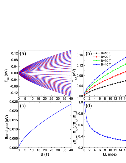
FIG. 1: (a) LLs as a function of magnetic field for the lowest fifteen sub-bands, where the blue solid (red dashed) lines indicate the numerical (analytical) results. (b) LLs in the conduction band varying with level index under different magnetic fields. (c) Band gap of the LL spectrum versus magnetic field. (d) LL spacings in the conduction band (blue line) in unit of the first one ($E_{c,1}-E_{c,0}$) as a function of level index under magnetic field $B=30$ T.

Another way to obtain the eigenvalues of Hamiltonian (4) is to use a semiclassical argument, e.g., the Sommerfeld quantization Dietl . The formula of LL spectrum is given as

$$E_{s,n}=sg(n)[\frac{\hbar v_{F}e}{\sqrt{m^{\ast}}}(n+\frac{1}{2})B]^{2/3},n=0,1,2,3,\cdots.$$ (6)

To determine the function $g(n)$, we need to fit Eq. (6) with the numerical data. In our work, we find $g(0)$=0.9454, $g(1)$=1.1668, and $g(n)$=1.1723 for $n$$\geqq$2. At this point, it is interesting to compare the LLs of 2D semi-Dirac electron systems with those of Schrödinger electrons in conventional semi-metal or semiconductors, and Dirac electrons in graphene. The results are summarized as

$$E_{n}=\left\{\begin{array}[]{c}\frac{\hbar eB}{m^{\ast}}(n+\frac{1}{2}):\text{Schr\"{o}dinger electrons}\\ \text{sgn}\left(n\right)v_{F}\sqrt{2e\hbar B\left|n\right|}:\text{Dirac electrons}\\ \text{sgn}(n)[\sqrt{\frac{\hbar eB}{m^{\ast}}}v_{F}\sqrt{e\hbar B}(|n|+\frac{1}{2})]^{2/3}:\text{Semi-Dirac electrons.}\end{array}\right.$$ (7)

Obviously, the LLs of the three kinds of two dimensional electron gas are different from each other. Further, the LL spacings for $n$$\geqq$2 are

$$\Delta E_{n} = E_{s,n+1}-E_{s,n}$$ (8)

$$= \frac{2\left(n+1\right)\epsilon_{0}}{(n+\frac{3}{2})^{4/3}+(n+\frac{1}{2})^{4/3}+(n+\frac{3}{2})^{2/3}(n+\frac{1}{2})^{2/3}},$$

where $\epsilon_{0}=\left(\hbar v_{F}eB/\sqrt{m^{\ast}}\right)^{2/3}.$

Figure 1(a) plots the LLs as a function of magnetic field for the lowest fifteen sub-bands. From Fig. 1(a), we find that the LLs (the red lines) given by Sommerfeld quantization [see Eq. (6)] perfectly reproduce the numerical results (blue lines) under any magnetic field. This proves that the LLs of 2D semi-Dirac electron system are proportional to the 2/3 power law of the magnetic field. Moreover, the LLs also show $2/3$ power law dependence on the level index under different magnetic fields [see Fig. 1(b)]. This $2/3$ power dependence on the magnetic field and level index is different from that in conventional semi-metals or semiconductors Stern ; Klitzing or Dirac materials KSNovoselov ; Zhangyuanbo ; Sadowski . Although semi-Dirac electrons are realized in potassium-doped few-layer black phosphorus Kim , the LLs are already quite different from those of pristine black phosphorus xyzhou1 ; xyzhou2 ; xyzhou3 ; yjjiang , indicating that they have become different electron systems. In contrast to the gapless LLs of Dirac materials KSNovoselov ; Zhangyuanbo ; Sadowski , there is a band gap in the LL spectrum due to the zero-point energy of the harmonic oscillator, which is more similar to that in conventional semiconductors Stern ; Klitzing . The band gap is $2E_{c,0}$ which increases with the $2/3$ power law of the magnetic field [see Fig. 1(c)]. The stronger the magnetic field, the larger the band gap. Further, Fig. 1(d) shows the LL spacings in the conduction band in unit of the first one ($E_{c,1}-E_{c,0}$) as a function of level index under magnetic field $B$=30 T. From Fig. 1(d), we find that the LL spacings decrease with increasing level index, which can also be inferred from Eq. (8). In other words, the higher the level index, the smaller the LL spacing. For high level index limitation ($n$$\rightarrow$$\infty$), the LL spacing vanishes.

Unlike the highly anisotropic dispersion at zero magnetic field [see Eq. (2)], the LLs of a 2D semi-Dirac electron system are independent of the wave vectors, and seem to be isotropic. However, the anisotropy of the LLs can be revealed from the wave functions. Figs. 2(a) and 2(b) plot the spatial probability distributions in different Landau gauges of the first and second LL, respectively. The probability distributions are calculated by using the finite difference method Smith which is not presented here. As plotted in Fig. 2, we find that the probability distribution exhibits strong anisotropy. It decays much faster along the $y$-direction (red lines) than that along the $x$-direction (blue lines). This means that electrons are more localized in the $y$-direction due to the larger effective mass along this direction. The highly anisotropic probability distribution (wave function) plays important role in the magneto-optical absorption spectrum of 2D semi-Dirac electron system as shall be discussed later.

To conclude this subsection, the LL spectrum of a 2D semi-Dirac electron can be understood as a hybridization of that of the Schrödinger and Dirac electron but with new features. In particular, the band gap arising from the zero-point energy is inherited from the Schrödinger electron, while the decreasing LL spacing is inherited from the Dirac electron. However, the 2/3 power law dependence on the magnetic field and level index as well as the highly anisotropic wave function are not embedded in the LL spectrum of Schrödinger and Dirac electron systems.

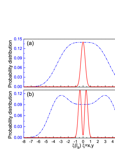
FIG. 2: (a)/(b) The spatial probability distributions of the first/second LLs in the conduction when choose different gauges for the vector potential $\mathbf{A}$. The blue/red lines represent the probability distribution along the $x/y$-direction.

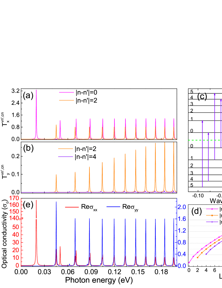
Fig. 3: (a)/(b) Nonzero elements of the interband transition rate as a function of photon energy for linearly polarized light along the $x$/$y$-direction with magnetic field $B=30$ T. (c) Schematic illustration of the interband magneto-optical transition rules, where the magenta, orange and purple arrows denote the interband transitions of $\Delta n=|n-n^{\prime}|=0,\pm 2,\pm 4$, respectively. (d) The photon energies of the three kinds of interband transitions with $|n-n^{\prime}|=0,\pm 2,\pm 4$ in unit of the band gap as a function of level index. (e) The real part of the longitudinal magneto-optical conductivity (in units of $\sigma_{0}=2e^{2}/h$) for interband transitions as a function of photon energy with magnetic field $B=30$ T.

II.2 Magneto-optical properties

Within the linear response theory, the dynamical conductivity can be written as TAndo1 ; Ando ; Lizhou ; Tabert

$$\sigma_{\mu\nu}(\omega)=\frac{\hbar e^{2}}{iS_{0}}\sum_{\xi\neq\xi^{\prime}}\frac{[f(E_{\xi})-f(E_{\xi^{\prime}})]\langle\xi|v_{\mu}|\xi^{\prime}\rangle\langle\xi^{\prime}|v_{\nu}|\xi\rangle}{(E_{\xi}-E_{\xi^{\prime}})(E_{\xi}-E_{\xi^{\prime}}+\hbar\omega+i\Gamma_{\xi})},$$ (9)

where $\hbar\omega$ is the photon energy, $S_{0}$$=$$L_{x}L_{y}$ the sample area with the size $L_{x}$ ($L_{y}$) in the $x$ ($y$)-direction, $|\zeta\rangle$$=$$|s,n,k_{x}\rangle$ the wavefunction expressed in Eq. (5), $f(E_{\xi})$$=$$[e^{(E_{\zeta}-E_{F})/k_{B}T}+1]^{-1}$ the Fermi-Dirac distribution function with Boltzman constant $k_{B}$ and temperature $T$. The sum runs over all states $|\xi\rangle$$=$$|s,n,k_{x}\rangle$ and $|\xi^{\prime}\rangle$$=$$|s^{\prime},n^{\prime},k_{x}^{\prime}\rangle$ with $\xi$$\neq$$\xi^{\prime}$. Meanwhile, $\Gamma_{\xi}\propto\sqrt{B}$ accounts for the LL broadening induced by the disorder effects TAndo1 ; Esfarjani . In the simplest approximation, we can assume the broadenings are the same for each LL. The velocity matrix operators $v_{x/y}$=$\partial H/\partial p_{x/y}$ are

$$v_{x}=v_{F}\sigma_{y},v_{y}=-iv_{0}(\hat{a}^{{\dagger}}-\hat{a})\sigma_{x},$$ (10)

where $v_{0}$=$\hbar/\sqrt{2}l_{B}m^{\ast}$. It is worth noting that the velocity operators are anisotropic which will result in a highly anisotropic magneto-optical absorption spectrum. Under moderate magnetic fields, the absorption for linearly polarized light along the $x$-direction is stronger than that along the $y$-direction because of $v_{F}>v_{0}$. Meanwhile, we note that $v_{x}$ ($v_{y}$) is independent (dependent) on the upper and lower operators, which means the magneto-optical transition selection rules may also be anisotropic. By using the wavefunction in Eq. (5), the transition matrix elements of the velocity matrices are

$$X_{n^{\prime},n}^{s^{\prime},s} = \left\langle s^{\prime},n^{\prime},k_{x}^{\prime}\left|v_{x}\right|s,n,k_{x}\right\rangle$$

$$= \sum_{m^{\prime},m}^{M}iv_{F}(-u_{m^{\prime}}^{n^{\prime},s^{\prime}\ast}v_{m}^{n,s}+v_{m^{\prime}}^{n^{\prime},s^{\prime}\ast}u_{m}^{n,s})\delta_{m^{\prime},m},$$

$$Y_{n,n^{\prime}}^{s,s^{\prime}} = \left\langle s,n,k_{x}\left|v_{y}\right|s^{\prime},n^{\prime},k_{x}^{\prime}\right\rangle$$ (11)

$$= \sum_{m,m^{\prime}}^{M}-iv_{0}(u_{m}^{n,s\ast}v_{m^{\prime}}^{n^{\prime},s^{\prime}}+v_{m}^{n,s\ast}u_{m^{\prime}}^{n^{\prime},s^{\prime}})$$

$$\times\left(-\sqrt{m}\delta_{m^{\prime},m-1}+\sqrt{m+1}\delta_{m^{\prime},m+1}\right).$$

By Fermi's golden rule Zettili ; Sari , the transition rate from the $n$-th LL in the $s$ band to the $n^{\prime}$-th one in the $s^{\prime}$ band for linearly polarized light along the $x$-direction is

$$T_{x}^{s^{\prime}n^{\prime},sn}=\frac{2\pi}{\hbar}\left(\frac{\hbar}{l_{B}}\left|X_{n,n^{\prime}}^{s,s^{\prime}}\right|\right)^{2}\delta\left(E_{s^{\prime}n^{\prime}}-E_{sn}\pm\hbar\omega\right)f(E_{s^{\prime}n^{\prime}})\left[1-f(E_{sn})\right],$$ (12)

while $T_{y}^{s^{\prime}n^{\prime},sn}$ is similar to $T_{x}^{s^{\prime}n^{\prime},sn}$. Hence, the normal of the matrix elements $|X_{n^{\prime},n}^{s^{\prime},s}|^{2}$ and $|Y_{n^{\prime},n}^{s^{\prime},s}|^{2}$ directly determine the magneto-optical transition selection rules. A zero matrix element represents a forbidden transition. Although the transition matrix elements [see Eq. (11)] can not be obtained analytically, we can still obtain the magneto-optical transition selection rules by numerically checking all the matrix elements of the transition rate one by one. With the velocity matrix elements in Eq. (11), one can evaluate the magneto-optical conductivity for linearly polarized light directly. Substituting Eq. (11) into Eq. (9) and making the replacement $\sum_{k_{x}}$$\rightarrow$$g_{s}S_{0}/2\pi l_{B}^{2}$, where $g_{s}$=2 for the spin degeneracy, we obtain the real (absorption) part of the longitudinal magneto-optical conductivity as

$$\frac{\text{Re}\sigma_{\mu\mu}}{\sigma_{0}}=\sum_{n,n^{\prime},s,s^{\prime}}\frac{[f(E_{n^{\prime},s^{\prime}})-f(E_{n,s})]|\mu_{n^{\prime},n}^{s^{\prime},s}|^{2}\Gamma}{(E_{n,s}-E_{n^{\prime},s^{\prime}})[(E_{n,s}-E_{n^{\prime},s^{\prime}}+\hbar\omega)^{2}+\Gamma^{2}]},$$ (13)

where $\mu$=($x,y$), $x_{n^{\prime},n}^{s^{\prime},s}$=$\hbar X_{n^{\prime},n}^{s^{\prime},s}/l_{B}$, $y_{n^{\prime},n}^{s^{\prime},s}$=$\hbar Y_{n^{\prime},n}^{s^{\prime},s}/l_{B}$, and $\sigma_{0}$=$2e^{2}/h$.

III Results and discussion

In this section, we present the numerical results and discussions for the magneto-optical conductivities. Hereafter, unless explicitly specified, the conductivities are all in units of $\sigma_{0}=2e^{2}/h$, temperature $T=1$K, Fermi energy $E_{F}=0$ for interband transitions, and level broadening $\Gamma$=0.05$\sqrt{B}$ in unit of meV.

In order to understand the magneto-optical absorption spectra, we firstly examine the interband magneto-optical selection rules determined by the matrix elements of the transition rate. Figs. 3(a) and 3(b) plot all the nonzero matrix elements of the transition rate for interband transition as a function of the photon energy. As shown in Figs. 3(a) and 3(b), the matrix elements $T_{x}^{vn,cn^{\prime}}$ ($T_{y}^{vn,cn^{\prime}}$) are nonzero only if the level indexes satisfy $|n-n^{\prime}|$=0,2 ($|n-n^{\prime}|$=2,4), which indicates that the interband magneto-optical selection rule for linearly polarized light along the $x$($y$)-direction is $\Delta n=0,\pm 2$ ($\pm 2,\pm 4$), where we have defined $\Delta n=n-n^{\prime}$. Surprisingly, the interband magneto-optical selection rule of semi-Dirac electron system is anisotropic. This is quite different from the dipole transition ($\Delta n$=$\pm 1$) in conventional semiconductors Laura and Dirac materials Ando ; Tabert ; Lizhou ; Gusynin ; Chizhova . It also differs from the isotropic selection rule in black phosphorus thin film xyzhou1 ; yjjiang in spite of the highly anisotropic dispersion therein. We have schematically illustrated the interband magneto-optical selection rules in Fig. 3(c), where the magenta, orange and purple arrows denote the interband transitions of $\Delta n=0,\pm 2,\pm 4$, respectively. Further, in low photon energy regime, there are well-resolved two-peak structures in the transition rate spectra arising from the two kinds of transitions, i.e., $\Delta n=0,\pm 2$ or $\Delta n=\pm 2,\pm 4$. However, the two peaks in the transition rate spectra tend to coincide with each other with increasing photon energy and finally merge together in high photon energy regime [see the purple and orange lines in Fig. 3(a)]. This is actually a reflection of the decreasing spacings in the LL spectrum plotted in Fig. 1(d). In particular, we plot the photon energies of the three kinds of allowed interband transitions $\Delta n=0,\pm 2,\pm 4$ as a function of level index in Fig. 3(d). As depicted in the figure, in low photon energy regime, only the lower LLs participate in the optical transitions. There is a large energy difference among the allowed transitions, which leads to separated peaks in the transition rate spectra [see Figs. 3(a) and 3(b)]. However, with the increase of photon energy, LLs with high index are involved in the optical transitions. The difference of the nearest resonance energies corresponding to the allowed transitions becomes smaller and smaller and finally fades away [see Fig. 3(d)] with the increase of the level index arising from the smaller LL spacings depicted in Fig. 1(d). This contributes to merged peaks in the transition rate spectra in high photon energy regime [see Figs. 3(a) and 3(b)]. Meanwhile, the transition rate shows strong anisotropy originating from the anisotropy of the LLs, i.e, the velocity operators and the wavefunctions. The $T_{x}^{vn,cn^{\prime}}$ is two orders of magnitude larger than $T_{y}^{vn,cn^{\prime}}$, resulting from the highly anisotropic velocity operators, which can also be inferred from the probability distributions plotted in Fig. 2.

With the help of the magneto-optical selection rule, now we can understand the magneto-absorption spectra easier. Fig. 3(e) presents the real part of the interband longitudinal magneto-optical conductivity as a function of photon energy under magnetic field $B$=30 T. As shown in Fig. 3(e), the resonance frequency of the conductivity peak varies from the mid-infrared to the far-infrared regime for $B$=30 T. Of course, the resonance frequencies can be modulated by varying the magnetic fields. Further, the interband magneto-optical absorption spectra exhibit strong anisotropy inherited from the highly anisotropic transition rate spectra. The Re$\sigma_{xx}$ (red line) is hundreds times larger than Re$\sigma_{yy}$ (blue line) resulting from the highly anisotropic band structure in the absence of magnetic field, i.e., the highly anisotropic velocities along different directions [see Eq. (10)]. Owing to the anisotropic magneto-optical selection rule, i.e., $\Delta n=0,\pm 2$ ($\Delta n$=$\pm 2,\pm 4$) for linearly polarized light along $x(y)$-direction, the conductivity peaks in Re$\sigma_{xx}$ do not exactly coincide with those in Re$\sigma_{yy}$. In low photon energy regime, we find well-resolved two-peak structures in Re$\sigma_{xx}$ (Re$\sigma_{yy}$) corresponding to the transitions of $\Delta n=0,\pm 2$ ($\Delta n$=$\pm 2,\pm 4$). With the increase of photon energy, LLs with high index are involved in the transition process. The differences of the nearest resonance energies corresponding to the allowed transitions ($\Delta n$=$0,\pm 2,\pm 4$) become smaller and smaller. They finally vanish in high photon energy regime [see Fig. 3(d)] resulting from the decreasing LL spacing plotted in Fig. 1(d). Therefore, although the selection rule hasn't changed, we can only find one conductivity peak in both Re$\sigma_{xx}$ and Re$\sigma_{yy}$ in high photon energy regime. Quantitatively, the first conductivity peak in Re$\sigma_{xx}$ is one order of magnitude larger than others indicating a strong absorption from $E_{v0}$ to $E_{c0}$. Other conductivity peaks in Re$\sigma_{xx}$ contributed by $\Delta n$=0 are of the same order to those contributed by $\Delta n$=$\pm 2$. In contrast, the conductivity peaks in Re$\sigma_{yy}$ contributed by $\Delta n$=$\pm 4$ are much smaller than those contributed by $\Delta n$=$\pm 2$, which is also in line with the transition rates shown in Fig. 3(b). Hence, Re$\sigma_{yy}$ is dominated by the transition of $\Delta n=\pm 2$.

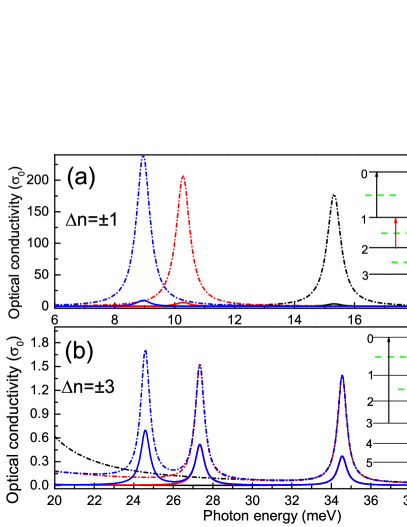
Fig. 4: The real part of the longitudinal magneto-optical conductivity as a function of the photon energy under magnetic field $B$=30 T for intraband transitions of (a) $\Delta n$=$\pm 1$ and (b) $\Delta n$=$\pm 3$, respectively. The dash-dotted (solid) lines denote the results for polarized light along the $x(y)$-direction. The insets depict the transitions between the nearest LLs for transitions with filling factor $\nu$=1 to 3. The color of the arrows is the same as that of the corresponding conductivity peaks.

Next, we turn to discuss the intraband transitions. Fig. 4 presents the real part of the longitudinal magneto-optical conductivity as a function of the photon energy under magnetic field $B$=30 T for intraband transitions with filling factor $\nu$=1 to 3. The dash-dotted (solid) lines denote the results for linearly polarized light along the $x(y)$-direction. In both Re$\sigma_{xx}$ and Re$\sigma_{yy}$, the intraband transitions occur when the level index changes as $\Delta n=\pm 1,\pm 3$, contributing to two groups of absorption peaks. This indicates that the magneto-optical selection rule of intraband transitions is independent of the direction of polarization of light, i.e, isotropic selection rules. This is the same as the magneto-optical selection rules for intraband transitions in black phosphorus thin films xyzhou1 . All the absorption peaks occur at the terahertz (THz) frequencies. We have schematically depicted the selection rules in the insets as the filling factor $\nu$ varying from 1 to 3. The color of the arrows in the insets is the same as that of the corresponding conductivity peaks. Although the selection rule is isotropic, the magneto-optical conductivity is still highly anisotropic. Re$\sigma_{xx}$ is one order of magnitude larger than Re$\sigma_{yy}$ because of the anisotropic velocity operator arising from the anisotropic dispersion at zero magnetic field. For certain Fermi level, the conductivity in both Re$\sigma_{xx}$ and Re$\sigma_{yy}$ contributed by the transition of $\Delta n$=$\pm 3$ is much smaller than that contributed by $\Delta n$=$\pm 1$. Therefore, the intraband conductivity is dominated by the dipole-type transitions ($\Delta n=\pm 1$). Under a fixed magnetic field, the resonant frequencies for the transitions of both $\Delta n$=$\pm 1$ and $\Delta n$=$\pm 3$ are red-shifted with the increase of filling factor (doping), which is a direct reflection of the decreasing LL spacings [see Fig. 1(d)]. The red-shift for the transitions of $\Delta n=\pm 3$ result in three-peak structures in the magneto-optical conductivity, which is more similar to the multi-peak structures in graphene Ando ; Gusynin ; Chizhova and silicene Tabert rather than the single peak structure in conventional semiconductors Laura . Moreover, the red-shift decreases with the magnetic field which can be understood from Eq. (8). Further, we would like to point out that the interband and intraband magneto-optical conductivities reported here can be directly measured through the infrared spectroscopy Sadowski ; Jiang or the magneto-absorption experiments Crassee .

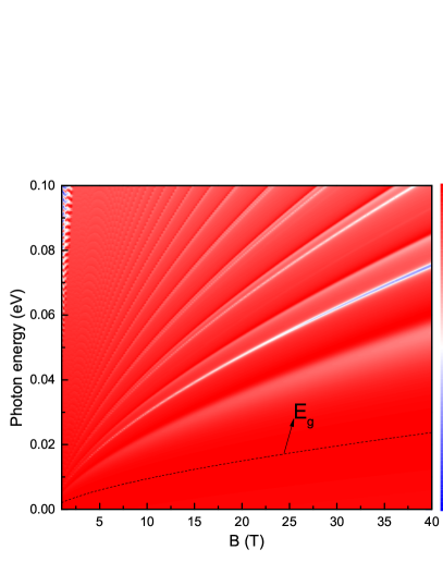
Fig. 5: Contour plot of the linear dichroism for interband transition as functions of photon energy and magnetic field. The black dashed line is the band gap of LL spectrum, which corresponds to the resonance energy of the perfect linear dichroism.

As discussed above, both the interband and intraband magneto-optical absorption spectra are highly anisotropic, which will result in a strong linear dichroism shuyunzhou ; Bentman ; Roth . We define a dimensionless parameter $I$=$(\mathrm{Re}\sigma_{xx}-\mathrm{Re}\sigma_{yy})/(\mathrm{Re}\sigma_{xx}+\mathrm{Re}\sigma_{yy})$ to indicate the linear dichroism quantitatively shuyunzhou . Fig. 5 presents a contour plot of the linear dichroism as a function of the photon energy and the magnetic field for the interband transitions. From the figure, we find that $I$ is larger than 0.8 within most photon energies and magnetic fields because Re$\sigma_{xx}$ is always dozens times larger than Re$\sigma_{yy}$. In principle, owing to the anisotropic selection rules, there should be a perfect linear dichroism for the photon energy corresponding to the transition of $\Delta n$=0 ($\Delta n$=$\pm 4$) which is only allowed in Re$\sigma_{xx}$ (Re$\sigma_{yy}$). However, the differences of the resonance photon energy between the transitions $\Delta n$=0 and $\Delta n$=$\pm 4$ are quenched in high photon energy regime [see Fig. 3(d)] where the perfect linear dichroism is destroyed. Fortunately, the perfect linear dichroism survives in low photon energy regime, where $I$ is always 1 resulting from the transition from $E_{v0}$ to $E_{c0}$, which only can be excited by linearly polarized along the $x$-direction. Importantly, the resonance energy of the perfect linear dichroism is exactly the band gap of LL spectrum, which can be effectively tunable by the magnetic field (see the black dashed line). Therefore, we can realize a perfect linear dichroism in 2D semi-Dirac materials with a magnetic field tunable wavelength by using the transition from $E_{v0}$ to $E_{c0}$, which is important to design new magneto-optical devices. There is also a strong linear dichroism for intraband transition of $\Delta n$=$\pm 1$. It is similar to that of interband transition in the high photon energy regime, and we do not present it here.

IV Summary

We have examined the LLs and magneto-optical absorption properties of a 2D semi-Dirac electron system based on an effective k$\cdot$p Hamiltonian and linear-response theory. We found that the LLs of 2D semi-Dirac electron system can be understood as a hybridization of those of the Schrödinger and Dirac electron but with new features. By using the Kubo formula, we found that the selection rules for interband magneto-optical transitions are anisotropic with $\Delta n$=$0,\pm 2$ ($\Delta n$=$\pm 2,\pm 4$) for linearly polarized light along the $x(y)$-direction. Whereas, the selection rules for intraband magneto-optical transitions are $\Delta n$=$\pm 1,\pm 3$ regardless of the polarization direction of light. For the interband (intraband) transition, the optical conductivity for linearly polarized light along the $x$-direction is two (one) orders of magnitude larger than that along the $y$-direction. The highly anisotropic magneto-optical absorption spectra clearly reflect the structure of the LLs and result in strong linear dichroism. The interband transition from $E_{v0}$ to $E_{c0}$ can realize a perfect linear dichroism with a magnetic field tunable wavelength. The magneto-absorption spectra occur at the infrared frequency and can be detected directly by the infrared spectroscopy Sadowski ; Jiang ; Crassee . Our results shed light on the magneto-optical properties of 2D semi-Dirac electron systems and pave the way to design magneto-optical devices based on it.

- (1) A. H. C. Neto, F. Guinea, N. M. R. Peres, K. S. Novoselov, and A. K. Geim, Rev. Mod. Phys. 81, 109 (2009).
- (2) N.P. Armitage, E.J. Mele, and Ashvin Vishwanath Rev. Mod. Phys. 90, 015001 (2018).
- (3) P. Dietl, F. Pichon, and G. Montambaux, Phys. Rev. Lett. 100, 236405 (2008).
- (4) G. Montambaux, F. Pichon, J.-N. Fuchs, and M. O. Goerbig, Phys. Rev. B 80, 153412 (2009).
- (5) S. Banerjee, R. R. P. Singh, V. Pardo, and W. E. Pickett, Phys. Rev. Lett. 103, 016402 (2009).
- (6) V. Pardo and W. E. Pickett, Phys. Rev. Lett. 102, 166803 (2009).
- (7) H. Huang, Z. Liu, H. Zhang, W. Duan, and D. Vanderbilt, Phys. Rev. B 92, 161115(R) (2015).
- (8) S. S. Baik, K. S. Kim, Y. Yi, and H. J. Choi, Nano Lett. 15, 7788 (2015).
- (9) Q. Liu, X. Zhang, L. B. Abdalla, A. Fazzio, and A. Zunger, Nano Lett. 15, 1222 (2015).
- (10) B. Ghosh, B. Singh, R. Prasad, and A. Agarwal, Phys. Rev. B 94, 205426 (2016).
- (11) H. Doh and H. J. Choi, 2D Mater. 4, 025071 (2017).
- (12) C. Wang, Q. Xia, Y. Nie, and G. Guo, J. Appl. Phys 117, 124302 (2015).
- (13) J. Kim, S. S. Baik, S. H. Ryu, Y. Sohn, S. Park, B. G. Park, J. Denlinger, Y. Yi, H. J. Choi, and K. S. Kim, Science 349, 723-726 (2015).
- (14) T. Makino, Y. Katagiri, C. Ohata, K. Nomura and J. Haruyama, RSC Adv. 7, 23427 (2017).
- (15) J. Jang, S. Ahn, and H. Min, 2D Mater. 6, 025029 (2019).
- (16) J. P. Carbotte, K. R. Bryenton, and E. J. Nicol, Phys. Rev. B 99, 115406 (2019).
- (17) S. Banerjee and W. E. Pickett, Phys. Rev. B 86, 075124 (2012).
- (18) F. Zhai, and J. Wang, J. Appl. Phys 116, 063704 (2014).
- (19) Wang Chen, Xianzhe Zhu, Xiaoying Zhou, and Guanghui Zhou, Phys. Rev. B 103, 125429 (2021).
- (20) Frank Stern and W. E. Howard, Phys. Rev. 163, 816 (1967).
- (21) K. von Klitzing, Rev. Mod. Phys. 58, 519 (1986).
- (22) K. S. Novoselov, A. K. Geim, S. V. Morozov, D. Jiang, M. I. Katsnelson, I. V. Grigorieva, S. V. Dubonos and A. A. Firsov, Nature 438, 197 (2005).
- (23) Yuanbo Zhang, Yan-Wen Tan, Horst L. Stormer and Philip Kim, Nature 438, 201 (2005).
- (24) M. L. Sadowski, G. Martinez, and M. Potemski, C. Berger and W. A. de Heer, Phys. Rev. Lett. 97, 266405 (2006).
- (25) Z. Jiang, E. A. Henriksen, L. C. Tung, Y.-J. Wang, M. E. Schwartz, M. Y. Han, P. Kim, and H. L. Stormer, Phys. Rev. Lett. 98, 197403 (2007).
- (26) I. Crassee, J. Levallois, A. L. Walter, M. Ostler, A. Bost-wick, E. Rotenberg, T. Seyller, D. Van Der Marel, and A. B. Kuzmenko, Nat. Phys. 7, 48 (2011).
- (27) Peng Cheng, Canli Song, Tong Zhang, Yanyi Zhang, Yilin Wang, Jin-Feng Jia, Jing Wang, Yayu Wang, Bang-Fen Zhu, Xi Chen, Xucun Ma, Ke He, Lili Wang, Xi Dai, Zhong Fang, Xincheng Xie, Xiao-Liang Qi, Chao-Xing Liu, Shou-Cheng Zhang, and Qi-Kun Xue, Phys. Rev. Lett. 105, 076801 (2010).
- (28) T. Hanaguri, K. Igarashi, M. Kawamura, H. Takagi, and T. Sasagawa, Phys. Rev. B 82, 081305(R) (2010).
- (29) Likai Li, Fangyuan Yang, Guo Jun Ye, Zuocheng Zhang, Zengwei Zhu, Wenkai Lou, Xiaoying Zhou, Liang Li, Kenji Watanabe, Takashi Taniguchi, Kai Chang, Yayu Wang, Xian Hui Chen and Yuanbo Zhang, Nat. Nanotech. 11, 593 (2016).
- (30) Xiaoying Zhou, Wen-Kai Lou, Feng Zhai and Kai Chang, Phys. Rev. B 92, 165405 (2015).
- (31) X. Y. Zhou, R. Zhang, J. P. Sun, Y. L. Zou, D. Zhang, W. K. Lou, F. Cheng, G. H. Zhou, F. Zhai and Kai Chang, Sci. Rep. 5, 12295 (2015).
- (32) Xiaoying Zhou, Wen-Kai Lou, Dong Zhang, Fang Cheng, Guanghui Zhou, and Kai Chang, Phys. Rev. B 95, 045408 (2017).
- (33) Yongjin Jiang, Rafael Roldán, Francisco Guinea, and Tony Low, Phys. Rev. B 92, 085408 (2015).
- (34) G. D. Smith, Numerical Solutions of Partial Differential Equations: Finite Difference Methods (Oxford Univ. Press, Oxford, 1978), 2nd ed.
- (35) T. Ando and Y. Uemura, J. Phys. Soc. Japan 36, 959 (1974).
- (36) Mikito Koshino and Tsuneya Ando, Phys. Rev. B 77, 115313 (2008).
- (37) C. J. Tabert and E. J. Nicol, Phys. Rev. Lett. 110, 197402 (2013).
- (38) Zhou Li and J. P. Carbotte, Phys. Rev. B 88, 045414 (2013).
- (39) K. Esfarjani, H. R. Glyde, and V. Sa-yakanit, Phys. Rev. B 41, 1042 (1990).
- (40) J. Sári, M. O. Goerbig, and Csaba Tőke, Phys. Rev. B 92, 035306 (2015).
- (41) N. Zettili, Quantum Mechanics: Concepts and Applications, 2nd ed. (Wiley, 2009).
- (42) Laura M. Roth, Benjamin Lax, and Solomon Zwerdling, Phys. Rev. 114, 90 (1959).
- (43) L. A. Chizhova, J. Burgdörfer, and F. Libisch, Phys. Rev. B 92, 125411 (2015).
- (44) V. P. Gusynin, S. G. Sharapov, and J. P. Carbotte, Phys. Rev. Lett. 98, 157402 (2007).
- (45) Changhua Bao, Hongyun Zhang, Teng Zhang, Xi Wu, Laipeng Luo, Shaohua Zhou, Qian Li, Yanhui Hou, Wei Yao, Liwei Liu, Pu Yu, Jia Li, Wenhui Duan, Hong Yao, Yeliang Wang, and Shuyun Zhou, Phys. Rev. Lett. 126, 206804 (2021).
- (46) H. Bentmann, H. Maaß, E. E. Krasovskii, T.R.F. Peixoto, C. Seibel, M. Leandersson, T. Balasubramanian, and F. Reinert, Phys. Rev. Lett. 119, 106401 (2017).
- (47) Ch. Roth, F. U. Hillebrecht, H. B. Rose, and E. Kisker, Phys. Rev. Lett. 70, 3479 (1993).