Task-Aware Few-Shot-Learning-Based Siamese Neural Network for Classifying Control-Flow-Obfuscated Malware

Abstract

Malware authors apply different techniques of control flow obfuscation, in order to create new malware variants to avoid detection. Existing Siamese neural network (SNN)-based malware detection methods fail to correctly classify different malware families when such obfuscated malware samples are present in the training dataset, resulting in high false-positive rates. To address this issue, we propose a novel task-aware few-shot-learning-based Siamese Neural Network that is resilient against the presence of malware variants affected by such control flow obfuscation techniques. Using the average entropy features of each malware family as inputs, in addition to the image features, our model generates the parameters for the feature layers, to more accurately adjust the feature embedding for different malware families, each of which has obfuscated malware variants. In addition, our proposed method can classify malware classes, even if there are only one or a few training samples available. Our model utilizes few-shot learning with the extracted features of a pre-trained network (e.g., VGG-16), to avoid the bias typically associated with a model trained with a limited number of training samples. Our proposed approach is highly effective in recognizing unique malware signatures, thus correctly classifying malware samples that belong to the same malware family, even in the presence of obfuscated malware variants. Our experimental results, validated by N-way on N-shot learning, show that our model is highly effective in classification accuracy, exceeding a rate >91%, compared to other similar methods.

Keywords Siamese neural network  $\cdot$ meta-learning  $\cdot$ malware classification  $\cdot$ code obfuscation  $\cdot$ few-shot learning

1 Introduction

Malware producers are ever more motivated to create new variants of malware, in order to gain profits from unauthorized information stealth. According to the malware detection agency AV Test (https://www.av-test.org/en/statistics/malware/ (accessed on 1 July 2021)), 100 million new variants of malware were generated from January to October 2020, which translates as roughly three thousand new malware daily.

In particular, we have witnessed the fast growth of mobile-based malware. An NTSC report published in 2020 https://www.ntsc.org/assets/pdfs/cyber-security-report-2020.pdf (accessed on 15 June 2021) reported that 27% of organizations globally have been impacted by malware attacks sent via Android mobile devices. In recent times, we have seen malware producers employ techniques such as obfuscation Dong et al. (2018); Chua and Balachandran (2018); Bacci et al. (2018) and repackaging Song et al. (2017); Lee et al. (2019); Zheng et al. (2017), mostly through the change of static features Zhu et al. (2018); Sun et al. (2017); Hu et al. (2014), to avoid detection. In response to the trend in the growth of mobile-based malware attacks, numerous Artificial Intelligence (AI)-based defense techniques have been proposed Vasan et al. (2020); Luo and Lo (2017); Su et al. (2018); Makandar and Patrot (2018); Hsiao et al. (2019); Singh et al. (2019).

We argue that there are two main issues to be addressed in the existing state-of-the-art of AI-based mobile malware attack defense.

The first issue is that most of the existing research tends to focus on learning from common semantic information about the generic features of malware families, and building feature embeddings Raff et al. (2018); Gibert et al. (2019); Shen et al. (2018). In this context, ’feature embedding’ means the features contained in a malware binary sample, which provide important clues as to whether the malware image—generated from the hexdump utility that displays the contents of binary files in hexadecimal, from which feature embedding is created—is malicious or not: if malicious, what type of malware family it belongs to is assessed, to build the right set of response strategies. These existing works often treat the fraction of the code changed by the obfuscation and repackaging as a type of noise Gibert et al. (2018), and thus tend to ignore the effect of the modification: this is largely because the code changed by the obfuscation and repackaging techniques displays a similar appearance when malware visualization techniques are applied Akarsh et al. (2019); Ni et al. (2018); Naeem et al. (2020). Using common semantic information as data input points to be fed into a deep neural network cannot capture the unique characteristics of each malware family signature: thus, they will not be able to accurately classify many variants arising from the same malware family Kalash et al. (2018); Milosevic et al. (2017); Vasan et al. (2020); Yuan et al. (2020), especially if an obfuscation technique is applied.

The second issue with the existing approaches is the demand for large data input, with which to find more relevant correlations across the features: such input is unable to detect and classify malware families trained with a limited number of samples (e.g., newly emerging variants of malware) Cao et al. (2018).

To address these two important issues, we propose a novel task-aware few-shot-learning based Siamese neural network, capable of detecting obfuscated malware variants belonging to the same malware family, even if only a small number of training samples are available.

The contributions of our proposed model are as follows:

• Our task-aware meta-learner network combines entropy attributes with image-based features for malware detection and classification. By utilizing the VGG-16 network as part of the meta-learning process, the weight generator assigns the weights of the combined features, which avoids the potential issue of introducing bias when the training sample size is limited;

• For the hybrid loss to compute the intra-class variance, the center loss is added alongside the constructive loss, to enable positive pairs and negative pairs to form more distinct clusters across the pairs of images processed by two CNNs;

• The results of our extensive experiments show that our proposed model is highly effective in recognizing the presence of a unique malware signature, despite the presence of obfuscation techniques, and that its accuracy exceeds the performance of similar methods.

We organized the rest of the paper as follows. We examine the related work in Section 2. We describe how control-flow-obfuscated malware variants are created, and we address why the generic SNN approach cannot detect such obfuscated malware variants in Section  3. We provide the details of our proposed model, along with the details of the main components, their roles and responsibilities, and an overview of the algorithm involved, in Section 4. In Section 5, we describe the details of the dataset, feature extraction, and the experimental results with analysis. Finally, we provide the conclusion to our work, including the limitations of our proposal, and future work directions, in Section 6.

2 Related Work

In this section, we review two lines of research relevant to our study: few-shot-learning-based malware detection and feature embedding applied for malware detection.

2.1 Entropy Feature in Feature Selection

Entropy value serves as a metric for feature selection, quantifying the information each feature contributes to the target variable or class. Selecting features with the highest information gain can enhance model performance and reduce overfitting. Huang et al. Huang et al. (2016) utilized the entropy function defined on sparse signal $x$ to recover such signals: minimizing it with an appropriate p-value yielded sparse solutions and improved signal recovery rates. Additionally, Finlayson et al. Finlayson et al. (2009) demonstrated that quadratic entropy values, being smoother and typically having a single minimum, offer the most efficient approach. This method aids full-color shadow removal, by comparing edges in the original and invariant images, followed by re-integration. Moreover, Allahverdyan et al. Kolouri et al. (2018); Allahverdyan et al. (2018) suggest that entropy minimization can lead to basic forms of intelligent behavior. Specifically, Kolouri et al. Kolouri et al. (2018) employed entropy minimization to bolster classifier confidence, while entropy regularization ensured that predictions remained close to unseen attributes in zero-shot tasks.

3 Preliminary

3.1 Control Flow Obfuscation

Malware obfuscation is a technique that is applied by malware authors to create new malware variants, in order to avoid detection without creating a completely brand-new malware signature. Among the many different obfuscation techniques, we focused on control flow obfuscation, which involves creating a new malware variant by reordering the control flow of functional logic from the original malware program Dong et al. (2018). This type of obfuscation technique makes the compiled malicious code appear to be different from the existing malware signature so that it can easily avoid detection. Our model can detect three different types of control flow obfuscation.

3.1.1 Function Logic Shuffling

This technique alters the control flow path of a malware program, by shuffling the order of function calls without affecting the semantics (i.e., purpose) of the original malware program: while the functionality between the original malware and the obfuscated version remains the same, the changing of appearance in the compiled code can result in the appearance of the malware image changing, and detection accuracy decreasing. An example is shown in Figure 1, where the order of function logic MyClass_2 and MyClass_3 is changed.

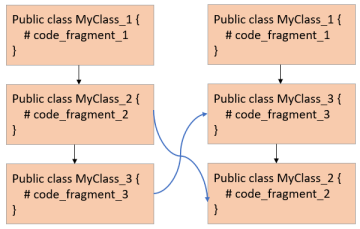
Figure 1: Function Logic Shuffling.

3.1.2 Junk Code Insertion

In this technique, the malware author inserts much (junk) code that never gets executed, whether after unconditional jumps, calls that never return, or conditional jumps with conditions that will never be met. The main goal of this technique is to change the control flow path, in order to avoid detection or to waste time for the reverse engineer analyzing useless code. An example of a junk code insertion is shown in Figure 2, where a junk code, MyClass_J, is added in between two normal function calls.

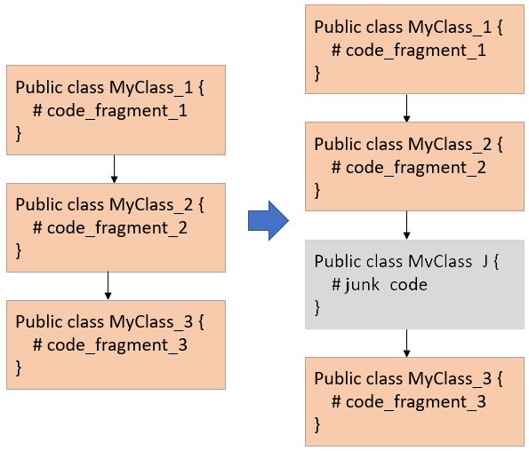
Figure 2: Junk Code Insertion.

3.1.3 Function Splitting

With this technique, the malware author applies the function splitting method, where a function code is fragmented into several pieces, each of which is inserted into the control flow. This technique splits the function into $n$ code fragments, or merges pieces of unrelated codes, to make the changes in the compiled code, which also results in the malware image appearance changing. An example of a function splitting is shown in Figure 3, where two splits from MyClass_2 are generated, and randomly added among other function calls.

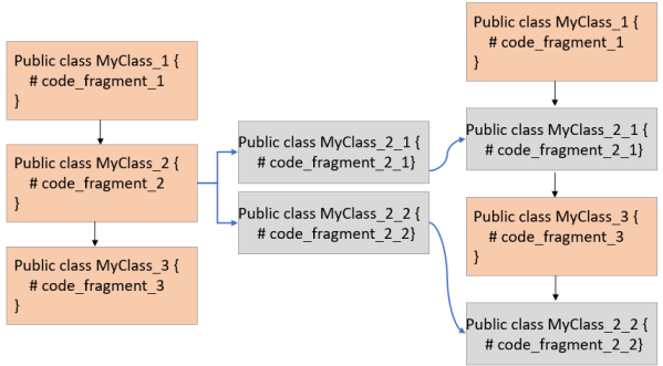
Figure 3: Function Splitting.

Though the functionality between the original malware and obfuscated versions (e.g., malware variants) stays the same, a malware code applied with control flow obfuscation can easily avoid detection from many anti-virus programs Dong et al. (2018). To address this issue, we propose a model resilient against the presence of many variants of malware created as a result of applying the control flow obfuscation technique. Our proposed method utilizes the information gain calculated through the entropy features associated with each malware variant. In our proposal, the entropy features measure the amount of uncertainty of a given probability distribution of a malware program that is not affected by the order of functional logic of the malware program.

3.2 Generic Approach and Issues

Table 1: Notations in task-aware meta learning-based Siamese neural network.

Notation	Description
$f_{p}$	The log probability calculated by the $d_{w}^{(i)}$.
$f_{q}$	The log probability calculated by the $1-d_{w}^{(i)}$.
$\mathbf{x_{i}}$	The malware image feature of $i$th samples.
$y_{t}^{i}$	The class $t$ of $i$th samples.
$\theta_{t}$	The feature layers’ parameters.
$\mathbf{W^{i}}$	I-th feature layer in $\mathcal{F}$’s weights.
$\mathbf{W^{i}_{sr}}$	The shared parameters for all malware families.
$\mathbf{W^{i}_{ts}}$	The task-specific parameters for each malware family.
$\mathbf{c_{i}}$	The center point of each class.
$L_{e}$	The embedding loss.
$L_{b,c}$	The binary cross entropy loss with center loss.
$\mathbf{d_{w}^{i}}$	The distance feature of a pair of images.
$y_{d}$	The label of pairs of images.
$\mathbf{F_{w}}$	The convolutional filter with parameters. $w$
$\beta$	The hyper-parameter.

In the last few years, few-shot learning technology, for example, the Siamese neural network (SNN), which uses only a few training samples to get better predictions has emerged. An SNN contains two identical subnetworks (usually convolutional neural networks)—hence the name ’Siamese’. The two CNNs have the same configuration, with the same weights, $\textbf{{W}}\in\mathbf{R}^{d}$, where W depicts the model’s parameters, while $\textbf{R}^{d}$ depicts the distance embedding to calculate two samples inputted from each subnetwork, respectively, and the value of the distance indicates whether they are closed to each other, as the value increases or decreases in the Euclidean space. The updating of the hyperparameters is mirrored across both CNNs, and is used to find the similarity of the inputs, by comparing its feature vectors.

Each parallel CNN is designed to produce an embedding (i.e., a reduced dimensional representation) of the input. These embeddings can then be used to optimize a loss function during the training phase and to generate a similarity score during the testing phase.

The architecture of Spiking Neural Networks (SNNs) contrasts significantly with traditional neural networks, which rely on extensive datasets to learn the prediction of multiple classes. The latter’s requirement for total retraining and updating with each addition or removal of a class presents a challenge. SNNs instead learn through a similarity function, testing whether two images are identical. This innovative architecture empowers them to classify new data classes without the need for additional network training. Furthermore, SNNs demonstrate greater robustness against class imbalance, as a small number of images per class is enough to enable future recognition. The corresponding notations are listed as Table 1.

Figure 4 illustrates the working of a generic SNN, its goal being to determine if two image samples belong to the same class or not: this is achieved through the use of two parallel CNNs (CNN1 and CNN2 in Figure 4) trained on the two image samples (Image 1 and Image 2 in Figure 4). Each image is fed through one branch of the SNN, which generates a d-dimensional feature embedding ($h_{1}$ and $h_{2}$ in Figure 4) for the image: it is these feature embeddings that are used to optimize a loss function, rather than the images themselves. A supervised cross-entropy function is used in the SNN for the binary classification, to determine whether two images are similar or dissimilar, by computing $[h_{2}$-$h_{1}]$ and processing it by a sigmoid function.

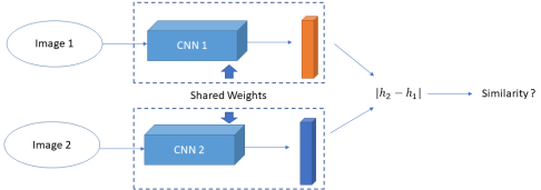
Figure 4: Overview of a Siamese neural network.

Mathematically, the similarity between a pair of images ($x_{1},x_{2}$) within Euclidean distance (ED) is computed in an SNN using the following equation:

$$\mathbf{d_{w}}(\mathbf{x_{1}},\mathbf{x_{2}})=\|F_{w}(\mathbf{x_{1}})-F_{w}(\mathbf{x_{2}})\|_{2},$$ (1)

where the $F_{w}$ indicates the feature representation for the inputted feature matrix. Generally, the model $g_{w}$: $\mathbf{R}^{n}$ to $\mathbf{R}^{d}$ is parameterized by the weights w, and its loss function is calculated using the following equation:

$$L_{b}=-\frac{1}{N}\sum_{i=1}^{N}[\mathbf{y^{i}_{d}}f_{p}(\mathbf{d_{w}^{(i)}})+(1-\mathbf{y_{d}^{i}})f_{q}(\mathbf{d_{w}^{(i)}})],$$ (2)

where $\mathbf{y_{d}}=\{\mathbf{y_{d}^{1},y_{d}^{2},\ldots,y_{d}^{i}}\}\in\{0,1\}$ denotes the ground truth label of image pairs ($\mathbf{x_{i},x_{j}}$), and $d_{w}$ represents the Euclidean distance (ED) between two images at the $i$-th pair. Note that the most similar images are supposed to be the closest in the feature embedding space: though this approach would work well for finding similarities/dissimilarities across distinct image objects, it would not work well for obfuscated malware samples.

Recall that an obfuscated malware—for example, $\mathbf{x_{1}}$—changes some part of the original malware code, $x_{2}$: when these two are converted as a feature representation—for example, $F_{w}(\mathbf{x_{1})}$ and $F_{w}(\mathbf{x_{2}})$—the feature values in the feature representation will look very different, which is how obfuscated malware avoids detection by anti-virus software. Inadvertently, the different values in the feature representation make the distance across obfuscated malware images very different from one another (i.e., $d_{w}(\mathbf{x_{1},x_{2}})$ is large). Eventually, when a similarity score is computed and compared, using the loss (i.e., $L_{b}$) based on the distance calculation (i.e., $d_{w}(\mathbf{x_{1},x_{2}})$), they appear to be different malware families—though, in fact, they all belong to the same malware family.

4 Task-Aware Meta Learning-Based Siamese Neural Network

We now introduce our task-aware meta-learning-based SNN model, which provides a novel feature embedding better-suited to control-flow-obfuscated malware classification. We start with the overview of our proposed model, and the details of the CNN architecture that is used by our model, followed by how task-specific weights are calculated using factorization. Finally, we discuss the details of the loss functions our model uses to address the challenges of weight generation with a limited number of training samples.

4.1 Our Model

As shown in Figure 5, our model utilizes a pre-trained network and two identical CNN networks. We use a pre-trained network (VGG-16) to compute more accurate weights for entropy features. Similarly, each CNN takes image features to calculate weight for the image features, and to generate feature embedding using the task-specific weights and shared weights of both the entropy and the image features. The feature embeddings produced by the two CNNs are used by the SNN to calculate the similarity score across intra-class variants, using a new hybrid loss function.

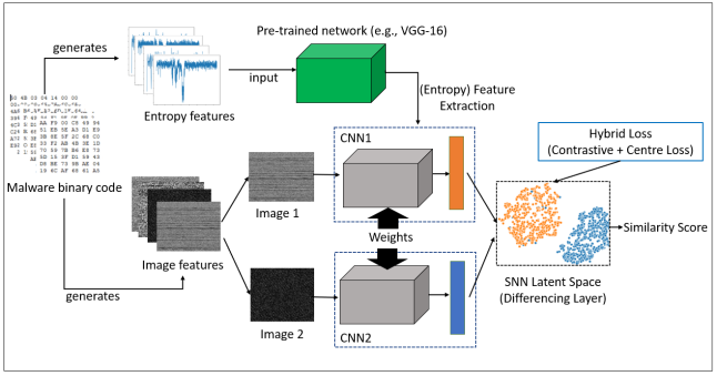
Figure 5: Overview of our proposed model.

Within each CNN, there are two sub-networks: a task-aware meta-learner network and an image network, as shown in Figure 6. The task-aware meta-learner network starts by taking a task specification (e.g., an entropy feature vector), and generates the weights. At the same time, the image network (e.g., a typical CNN branch of an SNN) starts by taking the image feature and convoluting it, until a fully connected layer is produced. The last fully connected layers use the weights generated by the task-aware meta-learner network, along with the shared weights, to produce a task-aware feature embedding space. Embedding loss for inter-class variance is calculated for back-propagation, until the CNN is fully trained for all input images.

Mathematically, this can be written as the following equation:

$$y=\mathcal{F}(x;\theta=\{\mathcal{G}(t),\theta_{f}\}),$$ (3)

where the SNN $\mathcal{F}$ takes malware images $\mathbf{x}$ as inputs, and produces a task-aware feature embedding that is used by the SNN to predict the similarity $\mathbf{y}\in\{1,0\}$ between an image pair inputted to two CNNs. Each CNN is parameterized by the weights $\theta$, which are composed of generated parameters from $\mathcal{T}$ and the share parameters $\theta_{s}$ in the SNN $\mathcal{F}$ that is shared across all malware families. The task-aware meta-learner network $\mathcal{T}$ creates a set of weight generators $g^{i},i={1\ldots k}$, to generate parameters for $k$ feature layers in $\mathcal{F}$, conditioned on $e_{t}$. The overall approach of our proposed model can also be summarized using Algorithm 1:

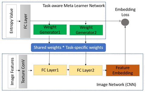
Figure 6: CNN architecture of our proposed model.

1 Binary cross-entropy with center loss:$L_{b,c}$;

2 Additional supervision loss :$L_{e}$;

3

Input : Entropy graph feature $F_{ent}$, texture feature $F_{t}$, support set $s$, query set $q$, pair label $y_{d}^{i}$, sample label $\mathbf{y_{t}^{i}}$, hyper-parameters $\beta$ , initialized centers $c_{i}$

Output : [Predicted similarity]

4

5Training stage:

6(1) Initializing the parameters for our proposed models, and the task-specific weights $W^{i}$ for the weight generators in the task-aware meta-learner network $g^{i}$, using the weight factorization Equation (5);

7(2) To input the malware texture features $F_{t}$ and the 4096 features of entropy value $F_{ent}$ extracted by the pre-trained network (e.g., VGG-16); note that these are integrated with the support set $s$ of our proposed model;

8(3) The weighted features from Equation (5) are fed into the embedding loss, according to the one-shot label generated from the target label;

9

10(4) Calculating the Euclidean distance (ED) of features in the two branches of SNN, through the hybrid loss function;

11 (5) Back-propagation and update parameters by Adam optimizer.

12

13Testing Stage:

14while not reach to iterations do

15       Extract features of samples in the query set $q$, and feed them the one-shot accuracy.

16Accuracy = 100$\times correct/iterations\;$

Algorithm 1 Pseudo-code of our proposed algorithm.

4.2 Task-Aware Meta-Learner

Our task-aware meta-learner provides two important functionalities: one is generating optimized task-specific weights, using the entropy values extracted from a pre-trained deep learning model (e.g., VGG-16); the other function is to work with the image network, to compute the new weights, based on the shared weights and the task-specific weights, so that the embedding loss is accurately calculated, in order to capture the relative distance across inter-class variance (e.g., the features of the image). These functions are necessary, because some malware samples (e.g., zero-day attack samples) are usually much smaller than the number of images required for training an SNN model.

Using the entropy values, our meta-learner recognizes a specific malware signature present in the entropy, so that later it uses this knowledge to find whether some malware samples are derived from the same malware family or not (e.g., obfuscated malware). The entropy values are extracted from the VGG-16 when entropy graphs are inputted.

We use entropy graphs to recognize a unique malware signature belonging to each malware family. To illustrate the use of an entropy graph as a task specification, four samples of malware images are shown in Figure 7. Figure 7a,b are two obfuscated malware samples from the same Wroba.wm family. Similarly, Figure 7c,d of the name Agent.ad are from the same Agent family. One can see that the entropy graphs within the same family share a similar pattern, while there are visible differences in the entropy graphs between two different malware families.

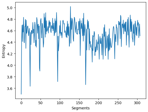
(a)

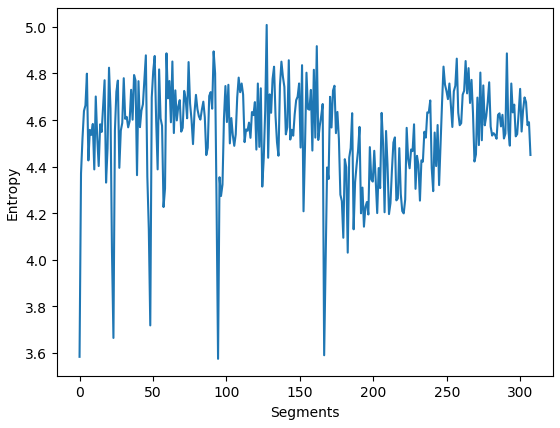
(b)

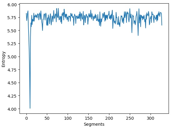
(c)

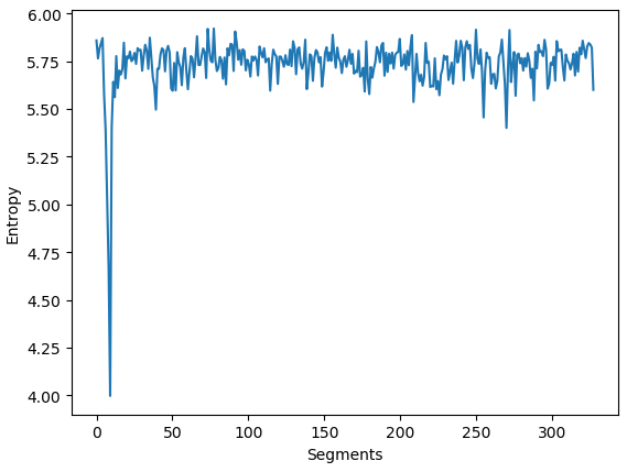
(d)

Figure 7: Examples of entropy graphs of two malware families.

Our task-aware meta-learner utilizes the entropy values extracted from the entropy graph, to train our proposed model to recognize if an image pair is similar or dissimilar (i.e., belong to the same malware family or not)—see Algorithm 2. To obtain an entropy graph, a malware binary file is read as a stream of bytes, and is separated into a few segments. The frequency of unique byte value is counted, and computes the entropy, using Shannon’s formula, as follows:

$$Ent=-\sum_{i}\sum_{j}M(i,j)logM(i,j)$$ (4)

where $M$ is the probability of an occurrence of a byte value. The entropy obtains the minimum value of 0 when all the byte values in a binary file are the same, while the maximum entropy value of 8 is obtained when all the byte values are different. The entropy values are then represented as a stream of values that can be reshaped as an entropy graph. The entropy graph is then converted as a feature vector inputted through the convolutional extractor of a pre-trained network (e.g., VGG-16 Simonyan and Zisserman (2014)). The summary of the steps involved in the entropy graph is described in Algorithm2:

1

Input : $f$: malware binary file; $l$: segment length; $n$: the number of files

Output : entropy graph matrix $m$

2

3while not reach to n do

4       1. read $l$ bytes from $f$, and defined as segment $s$;

5      2. for $i=0$ to $255$ do

6      3.     compute the probability $p_{i}$ of $i$ appearing in $s$;

7      

8      4.     compute the Shannon entropy

9

10Generate entropy graph $m$ 

Algorithm 2 Pseudo-code of entropy graph

4.3 Weight generator via factorization

In the generic SNN approach, the feature extractor only uses the image feature: this approach, however, is no longer effective in the detection of obfuscated malware, where multiple obfuscated malware samples contain almost identical image features.

The problem is further complicated when only a few samples (i.e., less than five malware samples) exist (i.e., not enough malware feature information to use for classification, as very few variations of malware samples can be collected from a small number of malware samples). To address this issue, we present a new novel weight generation scheme based on the work presented by Gidaris and Komodakis (2018). In our proposed model, the weight generator $G(.,.|\phi)$ receives, as input, the entropy vectors $\mathbf{W_{ave}}$ of a class, in addition to the image vectors $\mathbf{Z^{\prime}}={\{\mathbf{z^{{}^{\prime}}_{i}\}}_{i=1}^{N}}^{{}^{\prime}}$ of the $N^{\prime}$ training samples of the corresponding class: this results in a weight vector $\mathbf{w^{\prime}}=G(\mathbf{Z^{\prime},W_{ave})}$.

In our model, the weight generator scheme is incorporated in the fully connected (FC) layer, to solve the non-linear issue that exists in the relationship between the entropy feature and the malware image. By integrating the weight generator into the FC layer, the weights of the features extracted before the FC layer can then be integrated better into calculating new and more optimized weights for the whole model. We generate weights by creating a weight combination. The weight combination produces the composite features that encode the non-linear connection in the feature space: this is done by multiplying the entropy features and image features together, such that the composite features learn a feature-embedding resistance to different obfuscated malware variations. Note that the dimension of the weight generator $g^{i}$ on the FC layer must be matched with the dimension of the weight size of the $ith$ feature layers in $F$, so that the weights $\mathbf{W_{i}}\in\mathbf{R}^{m\times n}$ can be decomposed using the following equation:

$$W^{i}=W^{i}_{sr}\cdot W^{i}_{ts}$$ (5)

where $\mathbf{W^{i}_{sr}}\in\mathbf{R}^{m\times n}$ is the average entropy feature vector for each malware family $\{{t}_{1},\ldots{t}_{N}\}$, and $\mathbf{W^{i}_{ts}}\in$ $\mathbf{R}^{n}$ is the task-specific image feature vector for each malware. With such factorization, the weight generators only need to generate the malware-specific parameters for each malware family in the lower dimension, and learn one set of parameters in the high dimension shared across all malware families.

4.4 Loss Function

Our proposed model uses two different types of loss functions. Embedding loss is used by our task-aware meta-learner network to compute a loss across the inter-class variance (e.g., the features in the feature embedding space of a CNN branch), while a hybrid loss is used by the differencing layer of the SNN, to compute the similarities across inter-class variants between an image pair.

4.4.1 Embedding Loss for Meta-Learner

The feature representation of the entropy graph of a malware class can be easily influenced by binary loss: this is because the use of binary loss can only give the probability of the distribution of distances between positive and negative image pairs, and cannot estimate the probabilities of distances between positive and negative image pairs across different malware variations, thus not being able to correctly classify similar pairs of images across obfuscated malware samples (i.e., not being able to learn a discriminative feature during the training procedure). To address this issue, we added a secondary cross-entropy loss, not only to learn the discriminative feature, but also to address the effect of overfitting caused by contrastive loss. This embedding loss is defined using the following equation:

$$L_{e}=-\frac{1}{N}\sum^{N}_{i=1}\sum^{T}_{t=1}log[\frac{exp(F(\mathbf{x_{i}};\theta_{t}))\cdot\mathbf{y_{t}^{i}}}{\sum^{T}_{j=1}exp(F(\mathbf{x_{i}};\theta_{t}))}]$$ (6)

where $\mathbf{x^{i}}$ represents the $i$th sample in the dataset of the size $N$. The one-shot encoding applied to the input based on the labels is indicated by $\mathbf{y_{t}}$ $\in$ $\{0,1\}^{t}$, while $T$ indicates the number of tasks during training (e.g., either in the whole dataset or in the minibatch).

4.4.2 Hybrid Loss for Our SNN

To calculate the similarity score for our proposed model, we propose a hybrid loss function comprised of a center loss and a constructive loss. The center loss proposed by Wen et al. Wen et al. (2016) is a supplement loss function to the softmax loss for the classification task, which can learn to find a sample that can act as the center image of each class, and try to shorten the distance across the training samples of similar features by moving them to be as close to the center of the sample as possible. This center loss can be calculated as follows:

$$L_{c}=\frac{1}{2N}\sum_{N}^{i=1}\left\|\mathbf{d_{w}^{(i)}-c_{i}}\right\|_{2}^{2}$$ (7)

This approach, however, does not address the issue of moving apart from the training samples of dissimilar features. To address this issue, we propose the hybrid loss function integrated with the pairwise center, to better project the latent task embedding $e_{t}=T(t)$ into a joint embedding space that contains both the negative and positive center points.

We have adopted a metric learning approach, where the corresponding learned feature is closer to the joint feature embedding for positive inputs of a given image pair, while the corresponding learned feature is far away from the joint feature embedding for negative inputs of a given image pair:

$$\min L={\beta}\min L_{e}+L_{b,c}$$ (8)

where $\beta$ is the hyperparameter to balance the two terms; in our study, we set it at 0.8.

5 Experiments

In this section, we describe the details of the datasets we used for the experiments, the model configuration, and the results of our experiments. The results were obtained by running the experiments on a desktop with a 32 GM RAM, Nvidia Geforce RTX 2070(8GB), and Intel(R) Core(TM) i7-9700 CPU @ 3.00 GHz.

5.1 Andro-Dumpsys Dataset

We used the Andro-Dumpsys dataset obtained from wook Jang et al. (2016), which has been widely used for malware detection. The original dataset consists of 906 malicious binary files from 13 malware families. As illustrated in Table 2, the number of malware variants and the total number of samples from different malware families varied. Almost half of the malware families had no more than 25 malware samples, while some only had 1 sample, as they were most likely the new malware detected lately (e.g., Blocal and Newbak). In addition to the original dataset, we also generated three additional synthetic malware variants, each of which was applied using the different control flow obfuscation techniques described earlier: function logic shuffling; junk code insertion; and function splitting, respectively. Two samples from each additional malware variant, a total of 6 additional samples for each malware family, were added to the original dataset.

Table 2: Andro-Dumpsys Dataset with synthesis samples.

No.	Family	Number of Variants	Number of Samples
		(+3 Synthetic)	(+ 6 Synthetic)
1	Agent	39 (42)	150 (156)
2	Blocal	1 (4)	1 (7)
3	Climap	1 (4)	5 (11)
4	Fakeguard	1 (4)	10 (16)
5	Fech	1 (4)	3 (9)
6	Gepew	4 (7)	112 (118)
7	Gidix	6 (9)	108 (114)
8	Helir	1 (4)	15 (21)
9	Newbak	1 (4)	1 (7)
10	Recal	2 (5)	25 (31)
11	SmForw	23 (26)	166 (172)
12	Tebak	10 (13)	93 (99)
13	Wroba	23 (26)	108 (114)

Figure 8 illustrates a snippet of how obfuscated malware is created by applying a junk code insertion. In this example, we created a dummy array that acts as a junk code, which we added in between two function calls from the original malware code. We applied a similar approach to the other two types of control flow obfuscation.

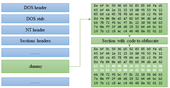
Figure 8: Example of inserting a junk code.

We also increased the image sample size, so as to have at least 30 samples for every malware family, using a data augmentation technique (e.g., applying random transformations, such as image rotations, re-scaling, and clipping the images horizontally). The details of the augmentation parameters are shown in Table 3. In particular, ZCA whitening is an image preprocessing method that leads to transformation of the data, such that the covariance matrix is the identity matrix, leading to decorrelated features, while the fill_mode argument with “wrap” simply replaces the empty area, and follows the filling scheme.

Table 3: Parameters of data augmentation.

Parameters	Values	Description
rescale	1./255	Resizing an image by a given scaling factor.
zca_epsilon	$1e^{-6}$	Epsilon for ZCA whitening.
fill_mode	wrap	Points outside the boundaries of the input are filled accord-
		ing to the given mode.
rotation_range	0.1	Setting degree of range for random rotations.
height_shift_range	0.5	Setting range for random vertical shifts.
horizontal_flip	True	Randomly flips inputs horizontally.

5.1.1 Image Feature

We used the same technique proposed by Zhu et al. (2020) to produce image features. To produce image features, we first read the binary malware as a vector of 8-bit unsigned integers, which were then converted into 2D vectors. We used the fixed width, while the height was decided according to the size of the original file. Finally, the 2D vector was converted into the gray images, using the color range [0, 255]. Note that the gray images at this stage were different dimensions according to the varying heights and widths in which size biases could occur in the fully connected layer: to address this issue, we used the bilinear interpolation method, as suggested by Malvar et al. (2004), to produce our image feature in uniform to the size of 105$\times$105.

5.1.2 Entropy Feature

To obtain the entropy feature of each malware family, we took each byte of the malware binary file as a random variable, and counted the frequency of each value (00h-FFh). More concretely, the byte reads from the binary file were divided into several segments. For each segment, we first calculated the frequency of each byte value $p_{j}(1\leq j\leq m)$, and then we calculated the entropy $y_{i}$ of the segment. The entropy values were then represented as a stream of values that could be reshaped as an entropy graph, with the size of $254\times 254\times 1$. These entropy graphs were then converted as a 4096-dimensional feature vector inputted through the convolutional extractor of the VGG-16 architecture Simonyan and Zisserman (2014).

5.2 Model Configurations

The task-aware meta-learner network $\mathcal{T}$(t) was a two-layer FC network with a hidden unit size of 512, except for the top layer, which was 4096 for input. The weight generator $g^{i}$ was a single FC layer with the output dimension the same as the output dimension of the corresponding feature layer in $\mathcal{F}$. We added a ReLU function to the output of $g^{i}$ in cases where processed malware images were used as inputs, and the convolutional part was configured as the 4-layer convolutional network (excluding pooling layers), following the same structure as Koch et al. (2015). In addition, the ReLU function and batch normalization were added afterwards by the convolution layer and the FC layer. The total number of parameters in our proposed model is 40 million. The overview of our network configurations is described in Figure 9.

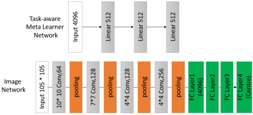
Figure 9: Network Configurations.

5.3 Results

We set the batch size to 32, and we used Adam as the optimizer, with an initial learning rate of $10^{-4}$ for the image network and the weight generators, and $10^{-5}$ for the task embedding network. The network was trained with 50 epochs, which ran for approximately 2 h. As Figure 10 illustrates, both train and validation loss stabilized after 50 epochs, confirming that the training had been done by this stage.

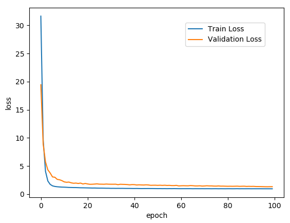
Figure 10: Loss during training on epochs.

The testing process conducted M times of N-way on N-shot learning tasks, where $Q$ times of correct predictions contributed to the accuracy, calculated by the following formula:

$$Accuracy=(100*Q/m)\%.$$ (9)

5.3.1 N-Way Matching Accuracy

The evaluation of $N$-way learning at each test state was carried out for one-shot and five-shot. For $N$-way one-shot learning, we chose an anchor image from one class of test, and then randomly selected $N$ classes of images to form the support set $X=\{x_{i}\}^{N}_{i=1}$, where $x_{1}$, $\forall x\in X$; the selected image’s class was the same as the anchor image $\hat{x}$, and the other images in the support sets were from different classes. The similarity score between $\hat{x}$ and other images was calculated using our model. Specifically, if the similarity score of the feature vector of $x_{1}$, which could be represented as $S=\{s_{i}\}^{N}_{i=1}$, was the maximum of $S$, then the task could be labeled as a correct prediction; otherwise, it was regarded as an incorrect prediction. For $N$-way five-shot learning, we randomly selected $N$ unseen classes and six instances, in which five instances of each class were randomly selected as the support set, $X=\{x_{1},\ldots,x_{i}\}^{N}_{i=5}$, and the remaining instances of each class formed the query set: its prediction procedure was the same as the test in the one-shot.

The matching accuracy of N-way accuracy for the one-shot and five-shot are illustrated in Figure 11. We randomly used 50 pairs of images, 25 containing positive image pairs and 25 containing negative image pairs, to test the effectiveness of our proposed model. As shown in the N-way one-shot result in Figure 11a, 19 out of 25 positive image pairs were matched correctly, while there were 6 true negatives (i.e., 2 positive pairs not matched correctly). Similarly, 23 of 25 negative pairs matched correctly, while there were 2 false positives (i.e., 2 negative pairs matched incorrectly). For the N-way five-shot results (shown in Figure 11b), the accuracy of matching was higher, as almost 22 out 25 pairs matched correctly for both positive and negative pairs, and there were 3 incorrectly matched results.

Figure 12 shows the projection of the embeddings space, using the two-dimensional principal component analysis (PCA) technique, where each orange point dictates the distance of a positive pair, while each blue point dictates the distance of a negative pair. Figure 12a shows the embedding space before training, while Figure 12b projects the embedding space after training. After training, we could clearly see two distinct clusters—one around the distance calculated for all positive pairs, and the other for negative pairs: this confirmed that our proposed model had learned well, so as to distinguish the similarities among positive pairs and negative pairs and separate them far apart.

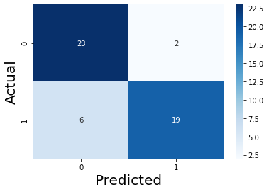
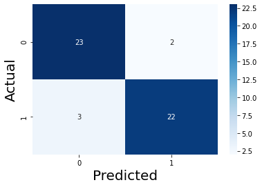
N-way one-shot	N-way five-shot

Figure 11: Matching Accuracy.

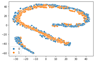
(a)

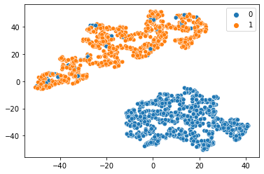
(b)

Figure 12: PCA visualization for classification performance.

5.3.2 Benchmark against similar methods

Table 4 shows the result of benchmarking our proposed model against the current state-of-the-art, especially the Matching network and Prototypical network, as well as the original Siamese network. Our model surpassed the performance of the Matching Network and Prototypical Network by $2.4\%$ and $1.8\%$ on the one-shot learning on the 5-way. The difference between our results of one-shot and five-shot was 3.1%, 1.9%, and 1.4% on the 5-way, 10-way, and 15-way, respectively. Our proposed five-shot result outperformed all three exiting models by 1.4%, 5.9%, and 5.4% on the 5-way, 10-way, and 15-way, respectively.

Table 4: Comparison of classification performance of different few-shot learning approaches for Andro-Dumpsys datasets.

1-shot
Ref	Method	5-way	10-way	15-way
Vinyals et al. (2016)	Matching network	85 $\pm$  2.2%	84 $\pm$  2.4%	76 $\pm$  2.6%
Snell et al. (2017)	Prototypical network	86 $\pm$  1.7%	82 $\pm$  1.7%	81 $\pm$  1.9%
Koch et al. (2015)	Siamese network	82 $\pm$  2.5%	69 $\pm$  2.3%	64 $\pm$  2.6%
	Task-aware SNN	88 $\pm$  2.2%	86 $\pm$  2.2%	82 $\pm$  2.4%
5-shot
Ref	Method	5-way	10-way	15-way
Vinyals et al. (2016)	Matching network	89 $\pm$  2.1%	86$\pm$  2.1%	78$\pm$  2.3%
Snell et al. (2017)	Prototypical network	89 $\pm$  1.2%	85$\pm$ 1.4%	82 $\pm$  1.5%
Koch et al. (2015)	Siamese network	85 $\pm$  2.0%	72 $\pm$  2.2%	69 $\pm$  2.7%
	Task-aware SNN	91$\pm$  1.8%	88$\pm$  2.1%	83 $\pm$  2.1%

5.3.3 Distance Measure Effectiveness

We also examined the effectiveness of our proposed model in distance measurement, by using the AUC (area under the curve) ROC (receiver operating characteristic) curve. The AUC–ROC curve is commonly composed of two performance measures: the true-positive (FPR) rate and the false-positive rate (FPR) rate. The equations related to these two performance measures of the AUC–ROC curve are shown as follows:

$$FPR(P^{*}):=\int_{p^{*}}^{1}f_{0}(p)dp,$$ (10)

$$TPR(P^{*}):=\int_{p^{*}}^{1}f_{1}(p)dp.$$

where the $f_{0}(p)$ is denoted by the probability of a density function for the predictions $p(x)$ produced by our proposed model. The negative pairs are labeled as 0, and $f_{1}(p)$ is the probability from the positive pair that is labeled as 1. The given discrimination threshold $P$ is the integrals of the tails of these distributions according to the true-positive rate and false-positive rate. Based on the two parameters TPR and FPR, the AUC–ROC curve is defined as follows:

$$AUC-ROC=\int_{0}^{1}TPR(FPR)D(FPR).$$ (11)

where the AUC measures the entire two-dimensional area underneath the entire ROC curve (i.e., integral calculus) from (0,0) to (1,1). For example, a model whose predictions are 100% wrong has an AUC of 0.0, while a model whose predictions are 100% correct has an AUC of 1.0. Using this concept, we demonstrated the result predicted by the saved weights of one-shot and five-shot, respectively, of the learned model on the test set, including 5-way, 10-way, and 15-way. These AUC–ROC curves are shown in Figures 13 and 14, which illustrate that the $\beta$ value at 0.8 provided the best performance when it was tested on one-shot N-way learning.

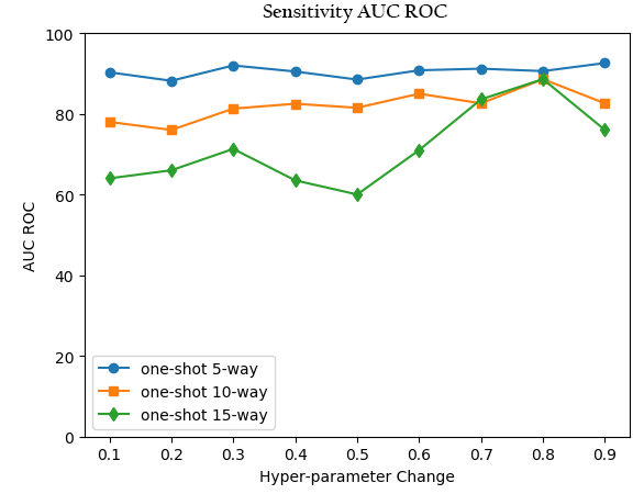
Figure 13: One-shot performance with hyperparameter changing.

This result also confirms that the hybrid multi-loss function can reduce the distance between the same classes, and enlarge the distance between different classes. Additionally, it does not change the attribute of the feature in the feature space, so the optimization of this layer will never negatively affect the deeper network layers. This hybrid loss function can also compute classification accuracy with a learned distance threshold on distances.

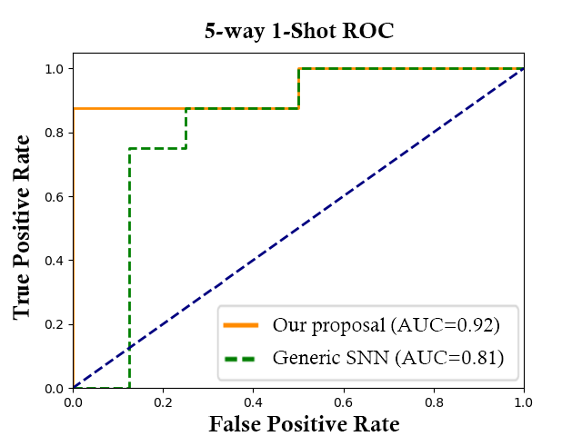
(a)

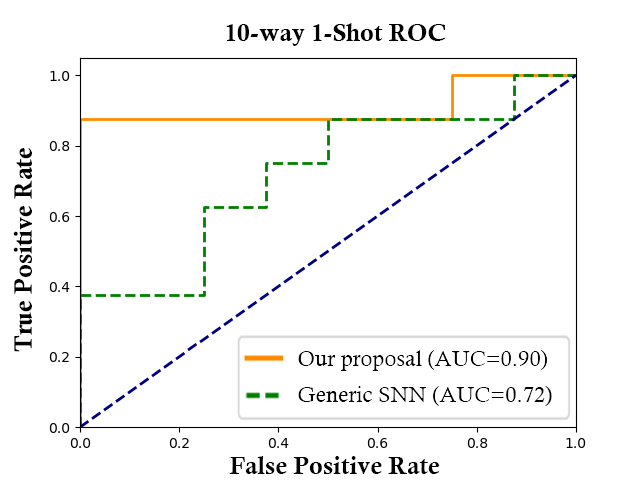
(b)

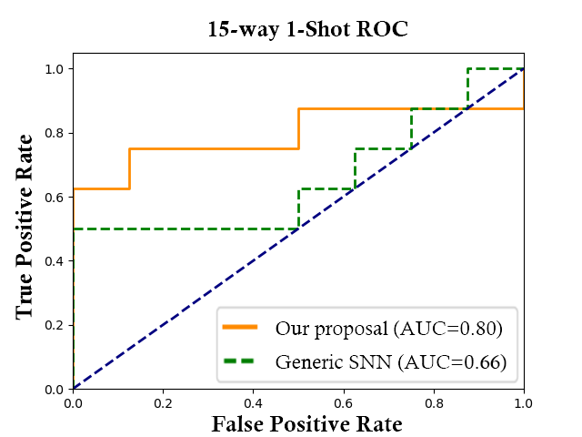
(c)

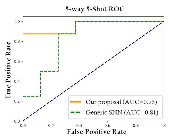
(d)

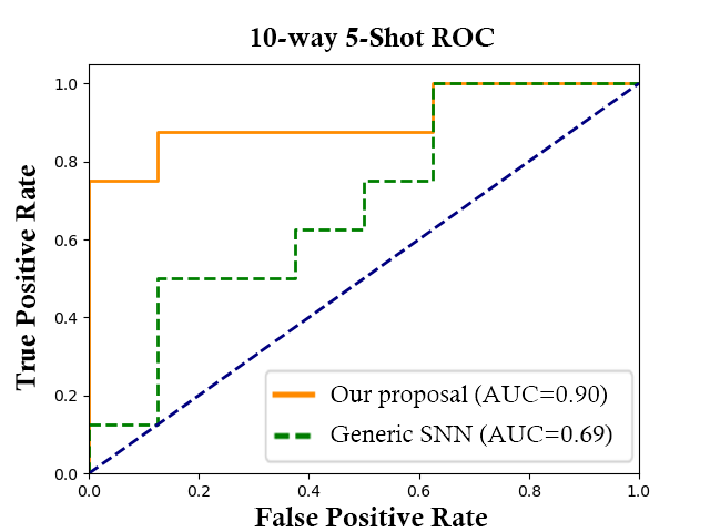
(e)

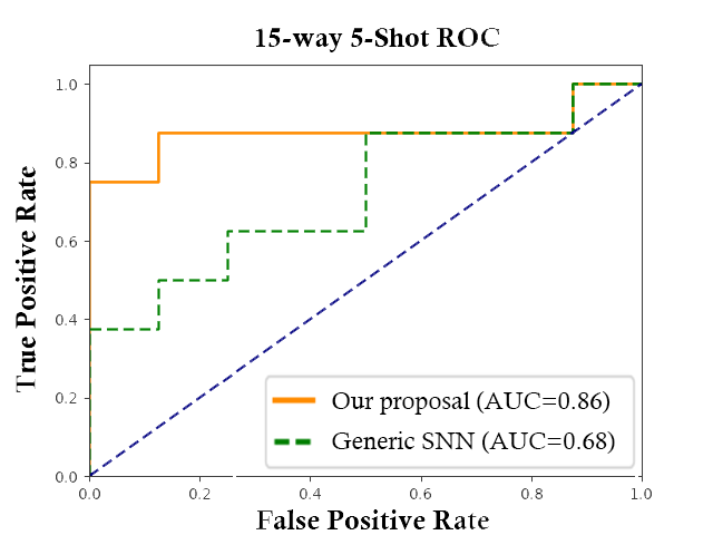
(f)

Figure 14: AUC–ROC curves under the N-way N-shot.

As shown, our result is on a set of points in the true positive rate–false positive rate plane. The results achieved an AUC–ROC equal to 0.92, 0.91, and 0.80, respectively, under the 5-way, 10-way, and 15-way on the one-shot learning. We further conducted the AUC–ROC on the five-shot learning. Our proposed model also obtained better performance than the generic SNN, with 95.6, 90.7, and 86.8 % at 5-way, 10-way, and 15-way, respectively. As expected, the accuracy of both one-shot and five-shot dropped as the number of N-way increased with higher intra-class variance.

Note that our model always performed better, as shown in these graphs, as the AUC–ROC areas (i.e., the areas up to the blue line) of our proposed model were larger compared to the generic SNN.

6 Conclusions

We propose a novel task-aware meta-learning-based Siamese neural network to accurately classify different malware families even in the presence of obfuscated malware variants. Each branch of the CNNs used by our model has an additional network called the “task-aware meta-learner network” that can generate task-specific weights, using the entropy graphs obtained from malware binary code. By combining the weight-specific parameters with the shared parameters, each CNN in our proposed model produces fully connected feature layers, so that the feature embedding in each CNN is accurately adjusted for different malware families, despite there being obfuscated malware variants in each malware family.

In addition, our proposed model can provide accurate similarity scores, even if it is trained with a limited number of samples. Our model also uses a pre-trained VGG-16 network in a meta-learning fashion, to compute accurate weight factors for entropy features. This meta-learning approach essentially solves the issues that are associated with creating potential bias due to not having enough training samples.

Our model also offers two different types of innovative loss functions that can more accurately compute the similarity scores within a CNN and the feature embeddings used by two CNNs.

Our experimental results show that our proposed model is highly effective in recognizing the presence of unique malware signatures, and is thus able to correctly classify obfuscated malware variants that belong to the same malware family.

We are planning to apply different types of malware samples (e.g., DDoS attack Wei et al. (2021) and ransomware families Zhu et al. (2021a, b); McIntosh et al. (2018, 2019)) and other data samples (e.g., finding similar abnormalities in medical X-ray images Feng et al. (2022)), to test the generalizability of our model.

References

- Dong et al. [2018] Shuaike Dong, Menghao Li, Wenrui Diao, Xiangyu Liu, Jian Liu, Zhou Li, Fenghao Xu, Kai Chen, Xiaofeng Wang, and Kehuan Zhang. Understanding android obfuscation techniques: A large-scale investigation in the wild. In International Conference on Security and Privacy in Communication Systems, pages 172–192. Springer, 2018.
- Chua and Balachandran [2018] Melissa Chua and Vivek Balachandran. Effectiveness of android obfuscation on evading anti-malware. In Proceedings of the Eighth ACM Conference on Data and Application Security and Privacy, pages 143–145, 2018.
- Bacci et al. [2018] Alessandro Bacci, Alberto Bartoli, Fabio Martinelli, Eric Medvet, and Francesco Mercaldo. Detection of obfuscation techniques in android applications. In Proceedings of the 13th International Conference on Availability, Reliability and Security, pages 1–9, 2018.
- Song et al. [2017] Lina Song, Zhanyong Tang, Zhen Li, Xiaoqing Gong, Xiaojiang Chen, Dingyi Fang, and Zheng Wang. Appis: Protect android apps against runtime repackaging attacks. In 2017 IEEE 23rd International Conference on Parallel and Distributed Systems (ICPADS), pages 25–32. IEEE, 2017.
- Lee et al. [2019] Yousik Lee, Samuel Woo, Jungho Lee, Yunkeun Song, Heeseok Moon, and Dong Hoon Lee. Enhanced android app-repackaging attack on in-vehicle network. Wireless Communications and Mobile Computing, 2019, 2019.
- Zheng et al. [2017] Xi Zheng, Lei Pan, and Erdem Yilmaz. Security analysis of modern mission critical android mobile applications. In Proceedings of the Australasian Computer Science Week Multiconference, pages 1–9, 2017.
- Zhu et al. [2018] Hui-Juan Zhu, Zhu-Hong You, Ze-Xuan Zhu, Wei-Lei Shi, Xing Chen, and Li Cheng. Droiddet: effective and robust detection of android malware using static analysis along with rotation forest model. Neurocomputing, 272:638–646, 2018.
- Sun et al. [2017] Bowen Sun, Qi Li, Yanhui Guo, Qiaokun Wen, Xiaoxi Lin, and Wenhan Liu. Malware family classification method based on static feature extraction. In 2017 3rd IEEE International Conference on Computer and Communications (ICCC), pages 507–513. IEEE, 2017.
- Hu et al. [2014] Xin Hu, Kent E Griffin, and Sandeep B Bhatkar. Encoding machine code instructions for static feature based malware clustering, September 2 2014. US Patent 8,826,439.
- Vasan et al. [2020] Danish Vasan, Mamoun Alazab, Sobia Wassan, Babak Safaei, and Qin Zheng. Image-based malware classification using ensemble of cnn architectures (imcec). Computers & Security, page 101748, 2020.
- Luo and Lo [2017] Jhu-Sin Luo and Dan Chia-Tien Lo. Binary malware image classification using machine learning with local binary pattern. In 2017 IEEE International Conference on Big Data (Big Data), pages 4664–4667. IEEE, 2017.
- Su et al. [2018] Jiawei Su, Danilo Vargas Vasconcellos, Sanjiva Prasad, Daniele Sgandurra, Yaokai Feng, and Kouichi Sakurai. Lightweight classification of iot malware based on image recognition. In 2018 IEEE 42Nd annual computer software and applications conference (COMPSAC), volume 2, pages 664–669. IEEE, 2018.
- Makandar and Patrot [2018] Aziz Makandar and Anita Patrot. Trojan malware image pattern classification. In Proceedings of International Conference on Cognition and Recognition, pages 253–262. Springer, 2018.
- Hsiao et al. [2019] Shou-Ching Hsiao, Da-Yu Kao, Zi-Yuan Liu, and Raylin Tso. Malware image classification using one-shot learning with siamese networks. Procedia Computer Science, 159:1863–1871, 2019.
- Singh et al. [2019] Abhishek Singh, Debojyoti Dutta, and Amit Saha. Migan: malware image synthesis using gans. In Proceedings of the AAAI Conference on Artificial Intelligence, volume 33, pages 10033–10034, 2019.
- Raff et al. [2018] Edward Raff, Richard Zak, Russell Cox, Jared Sylvester, Paul Yacci, Rebecca Ward, Anna Tracy, Mark McLean, and Charles Nicholas. An investigation of byte n-gram features for malware classification. Journal of Computer Virology and Hacking Techniques, 14(1):1–20, 2018.
- Gibert et al. [2019] Daniel Gibert, Carles Mateu, and Jordi Planes. A hierarchical convolutional neural network for malware classification. In 2019 International Joint Conference on Neural Networks (IJCNN), pages 1–8. IEEE, 2019.
- Shen et al. [2018] Jiayi Shen, Xianbin Cao, Yan Li, and Dong Xu. Feature adaptation and augmentation for cross-scene hyperspectral image classification. IEEE Geoscience and Remote Sensing Letters, 15(4):622–626, 2018.
- Gibert et al. [2018] Daniel Gibert, Carles Mateu, Jordi Planes, and Ramon Vicens. Classification of malware by using structural entropy on convolutional neural networks. In Proceedings of the AAAI Conference on Artificial Intelligence, volume 32, 2018.
- Akarsh et al. [2019] S Akarsh, Prabaharan Poornachandran, Vijay Krishna Menon, and KP Soman. A detailed investigation and analysis of deep learning architectures and visualization techniques for malware family identification. In Cybersecurity and Secure Information Systems, pages 241–286. Springer, 2019.
- Ni et al. [2018] Sang Ni, Quan Qian, and Rui Zhang. Malware identification using visualization images and deep learning. Computers & Security, 77:871–885, 2018.
- Naeem et al. [2020] Hamad Naeem, Farhan Ullah, Muhammad Rashid Naeem, Shehzad Khalid, Danish Vasan, Sohail Jabbar, and Saqib Saeed. Malware detection in industrial internet of things based on hybrid image visualization and deep learning model. Ad Hoc Networks, 105:102154, 2020.
- Kalash et al. [2018] Mahmoud Kalash, Mrigank Rochan, Noman Mohammed, Neil DB Bruce, Yang Wang, and Farkhund Iqbal. Malware classification with deep convolutional neural networks. In 2018 9th IFIP international conference on new technologies, mobility and security (NTMS), pages 1–5. IEEE, 2018.
- Milosevic et al. [2017] Nikola Milosevic, Ali Dehghantanha, and Kim-Kwang Raymond Choo. Machine learning aided android malware classification. Computers & Electrical Engineering, 61:266–274, 2017.
- Yuan et al. [2020] Baoguo Yuan, Junfeng Wang, Dong Liu, Wen Guo, Peng Wu, and Xuhua Bao. Byte-level malware classification based on markov images and deep learning. Computers & Security, 92:101740, 2020.
- Cao et al. [2018] Jie Cao, Zhe Su, Liyun Yu, Dongliang Chang, Xiaoxu Li, and Zhanyu Ma. Softmax cross entropy loss with unbiased decision boundary for image classification. In 2018 Chinese Automation Congress (CAC), pages 2028–2032. IEEE, 2018.
- Huang et al. [2016] Shuai Huang, Dung N Tran, and Trac D Tran. Sparse signal recovery based on nonconvex entropy minimization. In 2016 IEEE International Conference on Image Processing (ICIP), pages 3867–3871. IEEE, 2016.
- Finlayson et al. [2009] Graham D Finlayson, Mark S Drew, and Cheng Lu. Entropy minimization for shadow removal. International Journal of Computer Vision, 85(1):35–57, 2009.
- Kolouri et al. [2018] Soheil Kolouri, Mohammad Rostami, Yuri Owechko, and Kyungnam Kim. Joint dictionaries for zero-shot learning. In Proceedings of the AAAI conference on artificial intelligence, volume 32, 2018.
- Allahverdyan et al. [2018] Armen E Allahverdyan, Aram Galstyan, Ali E Abbas, and Zbigniew R Struzik. Adaptive decision making via entropy minimization. International Journal of Approximate Reasoning, 103:270–287, 2018.
- Simonyan and Zisserman [2014] Karen Simonyan and Andrew Zisserman. Very deep convolutional networks for large-scale image recognition. arXiv preprint arXiv:1409.1556, 2014.
- Gidaris and Komodakis [2018] Spyros Gidaris and Nikos Komodakis. Dynamic few-shot visual learning without forgetting. In Proceedings of the IEEE Conference on Computer Vision and Pattern Recognition, pages 4367–4375, 2018.
- Wen et al. [2016] Yandong Wen, Kaipeng Zhang, Zhifeng Li, and Yu Qiao. A discriminative feature learning approach for deep face recognition. In European conference on computer vision, pages 499–515. Springer, 2016.
- wook Jang et al. [2016] Jae wook Jang, Hyunjae Kang, Jiyoung Woo, Aziz Mohaisen, and Huy Kang Kim. Andro-dumpsys: Anti-malware system based on the similarity of malware creator and malware centric information. Computers Security, 58:125 – 138, 2016. ISSN 0167-4048. doi:http://dx.doi.org/10.1016/j.cose.2015.12.005. URL http://www.sciencedirect.com/science/article/pii/S016740481600002X.
- Zhu et al. [2020] Jinting Zhu, Julian Jang-Jaccard, and Paul A Watters. Multi-loss siamese neural network with batch normalization layer for malware detection. IEEE Access, 8:171542–171550, 2020.
- Malvar et al. [2004] Henrique S Malvar, Li-wei He, and Ross Cutler. High-quality linear interpolation for demosaicing of bayer-patterned color images. In 2004 IEEE International Conference on Acoustics, Speech, and Signal Processing, volume 3, pages iii–485. IEEE, 2004.
- Koch et al. [2015] Gregory Koch, Richard Zemel, and Ruslan Salakhutdinov. Siamese neural networks for one-shot image recognition. In ICML deep learning workshop, volume 2. Lille, 2015.
- Vinyals et al. [2016] Oriol Vinyals, Charles Blundell, Timothy Lillicrap, Koray Kavukcuoglu, and Daan Wierstra. Matching networks for one shot learning. arXiv preprint arXiv:1606.04080, 2016.
- Snell et al. [2017] Jake Snell, Kevin Swersky, and Richard S Zemel. Prototypical networks for few-shot learning. arXiv preprint arXiv:1703.05175, 2017.
- Wei et al. [2021] Yuanyuan Wei, Julian Jang-Jaccard, Fariza Sabrina, Amardeep Singh, Wen Xu, and Seyit Camtepe. Ae-mlp: A hybrid deep learning approach for ddos detection and classification. IEEE Access, 9:146810–146821, 2021.
- Zhu et al. [2021a] Jinting Zhu, Julian Jang-Jaccard, Amardeep Singh, Paul A Watters, and Seyit Camtepe. Task-aware meta learning-based siamese neural network for classifying obfuscated malware. arXiv preprint arXiv:2110.13409, 2021a.
- Zhu et al. [2021b] Jinting Zhu, Julian Jang-Jaccard, Amardeep Singh, Ian Welch, Harith AI-Sahaf, and Seyit Camtepe. A few-shot meta-learning based siamese neural network using entropy features for ransomware classification. arXiv preprint arXiv:2112.00668, 2021b.
- McIntosh et al. [2018] Timothy R McIntosh, Julian Jang-Jaccard, and Paul A Watters. Large scale behavioral analysis of ransomware attacks. In International Conference on Neural Information Processing, pages 217–229. Springer, 2018.
- McIntosh et al. [2019] Timothy McIntosh, Julian Jang-Jaccard, Paul Watters, and Teo Susnjak. The inadequacy of entropy-based ransomware detection. In International Conference on Neural Information Processing, pages 181–189. Springer, 2019.
- Feng et al. [2022] Sijing Feng, Qixiu Liu, Aakash Patel, Sibghat Ullah Bazai, Cheng-Kai Jin, Ji Soo Kim, Mikal Sarrafzadeh, Damian Azzollini, Jason Yeoh, Eve Kim, et al. Automated pneumothorax triaging in chest x-rays in the new zealand population using deep-learning algorithms. Journal of Medical Imaging and Radiation Oncology, 2022.