Abstract

We study supersymmetric inhomogeneous field theories in 1+1 dimensions which have explicit coordinate dependence. Although translation symmetry is broken, part of supersymmetries can be maintained. In this paper, we consider the simplest inhomogeneous theories with one real scalar field, which possess an unbroken supersymmetry. The energy is bounded from below by the topological charge which is not necessarily nonnegative definite. The bound is saturated if the first-order Bogomolny equation is satisfied. Non-constant static supersymmetric solutions above the vacuum involve in general a zero mode although the system lacks translation invariance. We consider two inhomogeneous theories obtained by deforming supersymmetric sine-Gordon theory and $\phi^{6}$ theory. They are deformed either by overall inhomogeneous rescaling of the superpotential or by inhomogeneous deformation of the vacuum expectation value. We construct explicitly the most general supersymmetric solutions and obtain the BPS energy spectrum for arbitrary position-dependent deformations. Nature of the solutions and their energies depend only on the boundary values of the inhomogeneous functions. The vacuum of minimum energy is not necessarily a constant configuration. In some cases, we find a one-parameter family of degenerate solutions which include a non-vacuum constant solution as a special case.

1 Introduction

Supersymmetry is usually studied as an extension of Poincare symmetry, but it can exist in theories where Poincare symmetry is not relevant or is partially broken. The latter appears if the theory has explicit coordinate dependence in the action. Such supersymmetric theories have been actively investigated recently. Janus Yang-Mills theories in four dimensions, where the gauge coupling depends on space, are dual to dilatonic deformations of AdS₅ space [1] and have been generalized to supersymmetric theories [2, 4, 3, 5, 6, 7, 8]. In three and four dimensions, mass-deformed ABJM and super Yang-Mills theories admit further deformations with inhomogeneous mass functions while some of supersymmetries are maintained [9, 10, 11, 12]. Gravity duals of those models were also discussed in [13, 14, 15, 16, 17, 11]. In two and three dimensions, supersymmetric theories with impurities were studied extensively [18, 19, 20, 21, 22, 23, 24, 26, 25]. Supersymmetric boundary/defect integrable models in two dimensions are also a subject of active research [27, 28, 29, 30, 31].

Supersymmetric field theories with Poincare invariance show many nice properties. For example, the energy is nonnegative definite [32, 33, 34]. In particular, the vacuum energy is zero if and only if it is annihilated by each of the supercharges. This directly comes from the fact that the Hamiltonian is the sum of the absolute squares of the supercharges.

Another important aspect of supersymmetric theories is the existence of BPS objects [35, 36] which preserve part of the supersymmetries of the theory. Imposing appropriate conditions on the supersymmetric parameter, one can obtain the first-order Bogomolny equation [36] which also minimizes the energy for a given topological sector. Classically, the solutions are lumps such as kinks, vortices, or monopoles, and the moduli space of the solutions reflects the underlying symmetry of the system.

In this paper, we will address these issues in supersymmetric theories where the translation symmetry is explicitly broken. For simplicity, we will restrict our interest only to two-dimensional classical supersymmetric theories with one real scalar multiplet. If the theories are Poincare-invariant, they have two supercharges in two dimensions. In case that the superpotential depends explicitly on space, one of the supersymmetries is explicitly broken but the other can still be maintained with the help of an additional term in the Lagrangian. We analyze the superalgebra of such case and show that the energy is bounded from below by the topological charge which can be negative. The bound is saturated if the Bogomolny equation is satisfied. Since it is a first-order differential equation, the general solution should have an integration constant. On the other hand, the energy of the solutions turns out to depend only on the boundary values of the superpotential. Therefore, the energy is independent of the integration constant and hence we can have a one-parameter family of supersymmetric solutions above the vacuum, i.e., the solution possesses a zero mode even though the system has no translation invariance. For a kink solution in usual homogeneous theories, the integration constant represents the position of the kink. For inhomogeneous theories considered in this paper, however, we will see that the physical interpretation of the constant depends on the nature of the solutions.

There would be, in principle, infinitely many different ways of deformation. In this paper, we consider two types of spatial dependence to the superpotential: an overall inhomogeneous rescaling of the superpotential and inhomogeneous deformation of the vacuum expectation. To be specific, we consider supersymmetric sine-Gordon (SSG) theory for the former deformation, and $\phi^{6}$ theory for the latter. Sine-Gordon theory is one of the most well-studied theories in $1+1$ dimensions and possesses many nice properties. It is particularly well-suited for our purpose in that it has an overall mass parameter in the potential which would be made inhomogeneous. Moreover, it has infinitely degenerate vacua and nontrivial solutions such as kinks and breathers. We will see how these features are affected by the inhomogeneous rescaling. We would like to mention that inhomogeneous rescaling of the potential has been studied in the context of BPS-impurity model especially for $\phi^{4}$ theory in [23]. We summarize and discuss the results of $\phi^{4}$ theory in our context in the appendix.

For the latter inhomogeneity, we investigate $\phi^{6}$ theory with a $\mathbb{Z}_{2}$ symmetry $\phi\rightarrow-\phi$. It can have three degenerate minima, one at $\phi=0$ and the others at nonzero values. Thus it is the simplest theory having both broken and unbroken vacua with $\mathbb{Z}_{2}$ symmetry. By varying the nonzero vacuum expectation values while keeping the minimum at $\phi=0$ intact, we can study how the inhomogeneity affect the spectrum of supersymmetric solutions. We will see that, with this kind of inhomogeneity, the minima of the potential or even the total number of minima depend on the position, and the vacuum profile needs not be constant in general, even though $\phi=0$ remains a legitimate supersymmetric solution with vanishing energy. This is to be contrasted with the former deformation where the vacuum is always given by constant configurations since the overall shape of the potential remains unchanged asymptotically.

For the deformed SSG and $\phi^{6}$ theories, even though they contain arbitrary position-dependent functions, we are able to construct explicitly the most general solutions of the Bogomolny equations. The BPS energy spectrum does not depend on the details of the inhomogeneity, but we will investigate how it changes according to the boundary values of the superpotential at spatial infinities. For the theories considered here, there are either two or three energy levels depending on the boundary values of the inhomogeneous function and the vacuum energy is negative. When there are two energy levels, the energy of non-constant solutions becomes degenerate with a constant solution and they together form a continuously deformable one-parameter family of solutions.

The rest of the paper is organized as follows. In section 2, we construct the supersymmetric Lagrangian with one real scalar multiplet in two dimensions where the superpotential depends on space. Then, from the superalgebra, we obtain the energy bound. We show that there is no universal lower bound in energy and that there exists a zero mode for non-constant supersymmetric solutions above the vacuum. In section 3, we consider theories obtained by inhomogeneous rescaling of the superpotential for the SSG theory. We explicitly solve the Bogomolny equation for an arbitrary inhomogeneous function and obtain the BPS energy spectrum. In section 4, we investigate inhomogeneous deformation of the vacuum expectation value in $\phi^{6}$ theory. We conclude in section 5 with a brief discussion on future research directions. In the appendix, we briefly discuss the inhomogeneous rescaling of $\phi^{4}$ theory.

2 Supersymmetric Inhomogeneous Field Theories

We begin with a brief review of two-dimensional $\mathcal{N}=1$ supersymmetric theories with a real scalar field. The action reads [37, 38],

$$S=\int d^{2}x\Big{[}-\frac{1}{2}\partial_{\mu}\phi\partial^{\mu}\phi+i\bar{\psi}\gamma^{\mu}\partial_{\mu}\psi+iW^{\prime\prime}(\phi)\,\bar{\psi}\psi-\frac{1}{2}W^{\prime}(\phi)^{2}\Big{]},$$ (2.1)

where $\phi$ is a real scalar field, $\psi$ a real Majorana fermion, $W(\phi)$ the superpotential, and $W^{\prime}\equiv\frac{dW}{d\phi}$. Here we follow the convention of the spinor indices in the Appendix of Ref. [9].

The theory (2.1) is invariant under the supersymmetric transformation,

$$\delta\phi=i\psi\epsilon,$$

$$\delta\psi=-\frac{1}{2}\gamma^{\mu}\partial_{\mu}\phi\,\epsilon+\frac{1}{2}W^{\prime}\epsilon,$$ (2.2)

where the supersymmetric parameter $\epsilon$ is a two-component real spinor and the gamma matrices are given by $\gamma^{\mu}=(i\sigma^{2},\sigma^{1})$ with $\mu=0,1$. The supercurrent is

$$J_{\epsilon}^{\mu}=-i\partial_{\nu}\phi\,\bar{\psi}\gamma^{\mu}\gamma^{\nu}\epsilon+iW^{\prime}\bar{\psi}\gamma^{\mu}\epsilon,$$ (2.3)

which leads to two supercharges,

$$Q_{\epsilon}=\int dxJ_{\epsilon}^{0}=i\epsilon_{+}Q_{+}+i\epsilon_{-}Q_{-}\quad{\rm with}\quad Q_{\pm} =\int dx\Big{(}(\partial_{0}\phi\pm\partial_{1}\phi)\psi_{\pm}\mp W^{\prime}\psi_{\mp}\Big{)},$$ (2.4)

where we set $\bar{\epsilon}^{\alpha}=(\epsilon_{+},\epsilon_{-})$ with $\bar{\epsilon}\equiv\epsilon^{\dagger}=\epsilon^{T}$. They satisfy the superalgebra,

$$\{Q_{\pm},Q^{\dagger}_{\pm}\}=2(P^{0}\mp P^{1}),\qquad\{Q_{\pm},Q_{\mp}^{\dagger}\}=2T,$$ (2.5)

where $P^{\mu}$ denotes the momentum and $T$ is the central charge of the superalgebra which is identified as the topological charge [33]

$$T=\int dx(\partial_{1}\phi)W^{\prime}(\phi)=\int dx\frac{dW(\phi(x))}{dx}=W(\phi(\infty))-W(\phi(-\infty)).$$ (2.6)

Accordingly, the energy can be written as

$$E=P^{0}=\frac{1}{4}\{Q_{+}\pm Q_{-},Q_{+}^{\dagger}\pm Q_{-}^{\dagger}\}\mp T.$$ (2.7)

It implies [33]

$$E\geq|T|,$$ (2.8)

which is manifestly nonnegative definite. In particular, the vacuum energy cannot be negative.

We would like to make a few remarks which seem trivial but will be relevant later. First, the nonnegativity of the energy in supersymmetric theories comes from the fact that it is bounded from below by both $T$ and $-T$ in two different ways. Each bound is saturated if the corresponding supercharge vanishes. Second, $T$ vanishes identically for constant configurations. This term is usually neglected when considering the vacuum energy since the vacuum is given by a constant configuration. We will later see how these features may be evaded in inhomogeneous theories which still have unbroken supersymmetries.

Now we consider the case that the superpotential depends explicitly on the position $W(\phi,x)$. For example, it may occur if some parameters in the superpotential depend on the coordinate $x$. Suppose that the supersymmetry transformation rule (2) remains unchanged except that the derivative of the superpotential $W^{\prime}$ is replaced by the partial derivative $\partial W/\partial\phi$ accordingly,

$$\delta\psi=-\frac{1}{2}\gamma^{\mu}\partial_{\mu}\phi\,\epsilon+\frac{1}{2}\frac{\partial W}{\partial\phi}\epsilon.$$ (2.9)

The action (2.1) is no longer invariant under this transformation but half of the supersymmetry can be preserved by adding a term in the Lagrangian,

$$\mathcal{L}=-\frac{1}{2}\partial_{\mu}\phi\partial^{\mu}\phi+i\bar{\psi}\gamma^{\mu}\partial_{\mu}\psi+i\frac{\partial^{2}W}{\partial\phi^{2}}\bar{\psi}\psi-\frac{1}{2}\left(\frac{\partial W}{\partial\phi}\right)^{2}\mp\frac{\partial W}{\partial x}.$$ (2.10)

It is straightforward to see that this theory is indeed invariant under the transformation (2.9) if $\epsilon$ satisfies

$$\gamma^{1}\epsilon=\pm\epsilon,$$ (2.11)

which implies $\epsilon_{-}=\pm\epsilon_{+}$. Similar projections for the supersymmetric parameters have been introduced in supersymmetric quantum field theories with inhomogeneous deformations in various dimensions [3, 5, 9, 20, 12]. In particular, Ref. [20] considered two-dimensional theories in the context of BPS preserving impurity models which we will compare with our approach later in this section.

For clarity, we choose the upper sign in the projection (2.11) from now on. Then the corresponding unbroken supercharge is given by

$$\bar{Q}_{\epsilon}=i\epsilon_{+}\bar{Q}$$ (2.12)

with

$$\bar{Q}=\int dx\Big{[}(\partial_{0}\phi+\partial_{1}\phi-\partial_{\phi}W)\psi_{+}-(\partial_{0}\phi-\partial_{1}\phi+\partial_{\phi}W)\psi_{-}\Big{]}.$$ (2.13)

By adding the last term in the Lagrangian in (2.10), we now have a position-dependent scalar potential

$$V(\phi,x)\equiv\frac{1}{2}\left(\frac{\partial W}{\partial\phi}\right)^{2}+\frac{\partial W}{\partial x},$$ (2.14)

which, in particular, need not be nonnegative definite. Then one can easily obtain

$$E=\frac{1}{4}\{\bar{Q},\,\bar{Q}^{\dagger}\}+T,$$ (2.15)

where the topological charge $T$ is defined in (2.6) with

$$\frac{dW}{dx}=\frac{\partial W}{\partial x}+\frac{\partial W}{\partial\phi}\frac{d\phi}{dx}.$$ (2.16)

This can also be directly seen by rewriting the bosonic part of the energy as

$$E =\int dx\left[\frac{1}{2}(\partial_{0}\phi)^{2}+\frac{1}{2}(\partial_{1}\phi)^{2}+\frac{1}{2}\left(\frac{\partial W}{\partial\phi}\right)^{2}+\frac{\partial W}{\partial x}\right]$$

$$=\int dx\left[\frac{1}{2}(\partial_{0}\phi)^{2}+\frac{1}{2}\left(\partial_{1}\phi-\frac{\partial W}{\partial\phi}\right)^{2}\right]+T.$$ (2.17)

The vacuum configuration is then time-independent, $\partial_{0}\phi=0$, and satisfies the first-order Bogomolny equation [36]

$$\frac{d\phi}{dx}-\frac{\partial W}{\partial\phi}=0,$$ (2.18)

as well as $\psi=0$. Equation (2.18) coincides with the Killing spinor equation $\delta\psi=0$, as it should be. It is also easy to check that every static solution of the Bogomolny equation satisfies automatically the second-order Euler-Lagrange equation. Moreover, the pressure density $T_{11}$, which is the spatial diagonal 11-component of the energy-momentum tensor, is given by

$$T_{11} =\frac{1}{2}(\partial_{0}\phi)^{2}+\frac{1}{2}(\partial_{1}\phi)^{2}-\frac{1}{2}\left(\frac{\partial W}{\partial\phi}\right)^{2}-\frac{\partial W}{\partial x}$$

$$=-\frac{\partial W}{\partial x},$$ (2.19)

where the Bogomolny equation (2.18) for static BPS configuration is used in the second line. Thus the pressure density of the static solution of (2.18) does not vanish but is given by the extra potential term, which is expected since the momentum is not conserved in inhomogeneous theories. In fact, it is easy to show that the momentum conservation is modified to

$$\partial_{0}T^{01}+\partial_{1}T^{11}=-\frac{\partial^{2}W}{\partial x^{2}}.$$ (2.20)

For static configurations, the first term in the left-hand side should vanish and hence this equation is consistent with (2).

In the conventional theory in which $W$ does not depend explicitly on the spatial coordinate $x$, the Bogomolny equation (2.18) is trivially satisfied by a constant configuration $\phi=\phi_{0}$ with $W^{\prime}(\phi_{0})=0$. Then the central charge vanishes, $T=0$, and the vacuum energy also vanishes. In inhomogeneous cases, however, $W(\phi,x)$ has nontrivial dependence on $x$ and there is no reason that the vacuum is given by a constant field configuration. Note also that the energy is bounded from below only by the topological charge $T$ itself as in (2.15) but not by its absolute value $|T|$. Therefore there is no guarantee that the energy is nonnegative definite even when the supersymmetry is unbroken.

There can be other solutions of (2.18) with higher energies above the vacuum. Then the supercharge of these solutions will vanish and the energy is again equal to the topological charge. Note, however, that (2.18) is a first-order differential equation and hence the solution will in general have an integration constant, say $c$, unless the solution is a constant configuration. Since the boundary values that $\phi$ can take at spatial infinities are in general discrete, the topological charge of the solutions are also discrete. Then the energy cannot depend on $c$ except some special case that $c$ alters the boundary values in some limit. In other words, variation of the integration constant $c$ should be a zero mode of the solution. Therefore the existence of the zero mode is a generic phenomenon for non-constant supersymmetric solutions above the vacuum even if the translation invariance of the theory is explicitly broken. In the following we will see how these are realized in explicit examples.

So far we have assumed that the kinetic term has the standard form as in (2.10). If we allow a more complicated form in the kinetic term including the coordinate dependence, we can generalize (2.10) to

$$\mathcal{L}=-\frac{1}{2}K^{2}\partial_{\mu}\phi\partial^{\mu}\phi+i\bar{\psi}\gamma^{\mu}\partial_{\mu}\psi+\frac{i}{K}\frac{\partial}{\partial\phi}\left(\frac{1}{K}\frac{\partial W}{\partial\phi}\right)\bar{\psi}\psi-\frac{1}{2}\left(\frac{1}{K}\frac{\partial W}{\partial\phi}\right)^{2}\mp\frac{\partial W}{\partial x},$$ (2.21)

where $K=K(\phi,x)$ is a function depending on both $\phi$ and $x$ and cannot be absorbed by a field redefinition. It is straightforward to check that this is invariant under the supersymmetric transformation,

$$\delta\phi =i\psi\epsilon,$$

$$\delta\psi =-\frac{1}{2}K^{2}\gamma^{\mu}\partial_{\mu}\phi\,\epsilon+\frac{1}{2}\frac{\partial W}{\partial\phi}\epsilon,$$ (2.22)

with (2.11). The energy is again bounded from below by $T$ and the bound is saturated if

$$K\frac{d\phi}{dx}\mp\frac{1}{K}\frac{\partial W}{\partial\phi}=0.$$ (2.23)

In this paper, we will only consider the case $K=1$ below.

A few remarks are in order. Supersymmetry in inhomogeneous theories in two dimensions was also considered in [20] to incorporate the BPS preserving impurity [21, 22] into supersymmetric theories. The most general bosonic Lagrangian considered in [20] is

$$\mathcal{L}=-\frac{1}{2}H^{2}\partial_{\mu}\phi\partial^{\mu}\phi-\frac{U}{H^{2}}-G^{2}-2\frac{\sqrt{U}G}{H}-\sqrt{2}HG\frac{\partial\phi}{\partial x},$$ (2.24)

where $H$ and $G$ are functions of $\phi$ and $\sigma$ such that $H\rightarrow 1$ and $G\rightarrow 0$ when $\sigma\rightarrow 0$. In our formulation, identifying $K$ in (2.21) with $H$ and $W=\sqrt{2}\int(\sqrt{U}+HG)d\phi$, we can readily see that the bosonic part of (2.21) reduces to (2.24) up to a total derivative $\frac{d}{dx}\int HG\,d\phi$. The separation of $U(\phi)$ and $G(\phi,\sigma)$ in [20] is physically motivated to represent $G$ as the impurity effect. From the viewpoint of general inhomogeneous field theories, however, such separation is not needed; the position-dependent superpotential $W(\phi,x)$ (and $K(\phi,x)$) is enough to incorporate impurities as well as more general inhomogeneous cases which we will consider in this paper.

Closing this section, we would like to note that the value of the energy in inhomogeneous case has no absolute meaning just as in usual nonsupersymmetric theories. This is because one can always add a field-independent term $W_{1}(x)$ to the superpotential which has no physical effect,

$$W(\phi,x)\longrightarrow W(\phi,x)+W_{1}(x).$$ (2.25)

Then the overall energy of the theory would be shifted by $\Delta E=W_{1}(\infty)-W_{1}(-\infty)$ and hence the energy can be made to take any value with a suitable choice of $W_{1}$. In particular, there is no universal lower bound of energy. In the following we will not add any field-independent term to the superpotential, i.e., we assume that every term in $W$ depends nontrivially on $\phi$, which would then provide a natural choice of energy in many cases. Also, one can add a total derivative term $\frac{d}{dx}F(\phi(x),x)$ to the Lagrangian as seen above, which would shift the energy by $F(\phi(\infty),\infty)-F(\phi(-\infty),-\infty)$. Then in theories with nontrivial boundary values of the field, the energy spectrum can change by adding this term, since solutions belonging to different topological sectors would give different energy shifts. This kind of ambiguity, however, exists even in usual homogeneous theories. We fix the ambiguity by requiring that there would be no linear term in $\partial_{x}\phi$ as in usual homogeneous theories, and also that the energy should coincide with that of the usual expression in the homogeneous limit. In any case, it would not produce any real physical effect ultimately. In particular, in the present case, it is evident that the central charge $T$ is also shifted by the same amount in (2.15), cancelling the energy shift.

3 Inhomogeneous Rescaling of Superpotential in Supersymmetric Sine-Gordon Theory

Having constructed the general inhomogeneous supersymmetric Lagrangian, we now discuss some specific class of inhomogeneities and their consequences. In this section we consider the theory obtained by inhomogeneous rescaling of the superpotential. Thus it can be applied to any superpotential. The same inhomogeneity has been considered by [23, 24] in the context of BPS-impurity model and detailed analysis has been performed with $\phi^{4}$ theory in particular for the dynamical aspects [26]. In this section, we would like to discuss the energy spectrum of supersymmetric solutions and consider the deformation of the SSG theory.

Given a superpotential $W_{0}(\phi)$, let

$$W(\phi,x)=g(x)W_{0}(\phi)$$ (3.26)

be the deformed superpotential where $g(x)$ is a position-dependent rescaling parameter. We assume that it goes to some nonzero finite values at spatial infinities so that the interaction does not vanish at infinities. Then the corresponding deformed potential is

$$V(\phi,x)=\frac{1}{2}g^{2}(x)\left(\frac{dW_{0}}{d\phi}\right)^{2}+g^{\prime}(x)W_{0}(\phi).$$ (3.27)

The Bogomolny equation (2.18) becomes

$$\phi^{\prime}(x)-g(x)W^{\prime}_{0}(\phi)=0.$$ (3.28)

Under the coordinate transformation from $x$ to $G(x)=\int g(x)dx$, (3.28) reduces to the undeformed form. Thus the rescaling of the superpotential is always solvable irrespective of an arbitrary function $g(x)$ [23]. Note that the boundary condition for $\phi(x)$ at spatial infinities is the same as that of the undeformed theory, i.e. they are extremum points of $W_{0}(\phi)$.

Let $\phi_{i}$ be extremum points of $W_{0}(\phi)$, and denote the boundary values of $g(x)$ as $g(\infty)=g_{R}$ and $g(-\infty)=g_{L}$. Then the constant configurations $\phi=\phi_{i}$ are obvious solutions of (3.28) and the corresponding energies are

$$E_{\phi=\phi_{i}} =T$$

$$=g(\infty)W_{0}(\phi(\infty))-g(-\infty)W_{0}(\phi(-\infty))$$

$$=(g_{R}-g_{L})W_{0}(\phi_{i}).$$ (3.29)

The vacuum energy is the minimum of these energies, $E_{\textrm{vac}}=\min_{\phi_{i}}E_{\phi=\phi_{i}}$. Note that, in this expression, the value of superpotential at the vacuum $W(\phi_{i})$ appears explicitly in the vacuum energy due to inhomogeneity of the parameter $g(x)$.

As an example, let us now consider the SSG theory  with inhomogeneous mass $m(x)$ of which the potential is

$$V=2\frac{m(x)^{2}}{\beta^{2}}\sin^{2}\frac{\beta\phi}{2}-4\frac{m^{\prime}(x)}{\beta^{2}}\cos\frac{\beta\phi}{2},$$ (3.30)

where $\beta$ is a constant and the mass $m(x)$ plays the role of the deformation parameter $g(x)$ in (3.27). The superpotential $W_{0}$ in (3.26) is

$$W_{0}(\phi)=-\frac{4}{\beta^{2}}\cos\frac{\beta\phi}{2},$$ (3.31)

which supports infinitely many extrema at

$$\phi_{n}\equiv\frac{2n\pi}{\beta},\qquad n\in\mathbb{Z},$$ (3.32)

with

$$W_{0}(\phi_{n})=(-1)^{n+1}\frac{4}{\beta^{2}}.$$ (3.33)

The Bogomolny equation (3.28) becomes

$$\frac{d\phi}{dx}=\frac{2m(x)}{\beta}\sin\frac{\beta\phi}{2}.$$ (3.34)

The constant configurations (3.32) trivially satisfy the Bogomolny equation and have energies

$$E_{\phi_{n}}=(-1)^{n+1}\frac{4}{\beta^{2}}(m_{R}-m_{L}),$$ (3.35)

where we have introduced $m_{R}=m(\infty)$ and $m_{L}=m(-\infty)$. The vacuum energy is the minimum of them,

$$E_{\textrm{vac}}=-\frac{4}{\beta^{2}}|m_{R}-m_{L}|,$$ (3.36)

which is negative unless $m_{L}=m_{R}$, and corresponds to the half of the constant configurations in (3.32),

$$\phi(x)=\phi_{2n+\delta},\qquad(n\in\mathbb{Z}),$$ (3.37)

where $\delta=\theta(m_{L}-m_{R})$. Therefore, the degeneracy of the constant configurations (3.32) in the original homogeneous theory is lifted unless $m_{L}=m_{R}$. This is of course because the second term in the potential (3.27) is periodic in $\frac{4\pi}{\beta}$, which is twice the period of undeformed theory. These vacua preserve supersymmetry of the theory even though the vacuum energy (3.36) is not zero. The other half of constant solutions $\phi(x)=\phi_{2n+1-\delta}$ have positive energy $E_{1}\equiv|E_{\textrm{vac}}|$.

Now we look for other solutions of (3.28) which are not constant. Let $\mu(x)$ be an integral of the mass function $m(x)$,

$$\mu(x)=\int_{0}^{x}m(x^{\prime})dx^{\prime}.$$ (3.38)

Then (3.28) can easily be integrated to

$$\phi(x)=\frac{4}{\beta}\tan^{-1}[c\,e^{\mu(x)}]\pmod{\tfrac{4\pi}{\beta}},$$ (3.39)

where $c$ is an integration constant. In homogeneous theories, one need not consider $c<0$ case since the period is $\frac{2\pi}{\beta}$. In the present case, however, we should also take $c<0$ case into account because, for example, the region $(-\frac{2\pi}{\beta},0]$ of $\phi$ cannot be identified with the region $(0,\frac{2\pi}{\beta}]$. For convenience, we assume that $\phi$ is in the range $(-\frac{2\pi}{\beta},\frac{2\pi}{\beta}]$, unless otherwise stated.

To understand the nature of solutions, we need to study the asymptotic behavior of $\mu(x)$,

$$\mu(x)\rightarrow m_{R/L}x+\cdots,\qquad x\rightarrow\pm\infty.$$ (3.40)

If $m_{L}>0$ and $m_{R}>0$, the solution (3.39) goes asymptotically to

$$\phi(x)\rightarrow\begin{cases}\begin{array}[]{ll}0,&x\rightarrow-\infty,\\ \varepsilon_{c}\frac{2\pi}{\beta},&x\rightarrow\infty,\end{array}\end{cases}$$ (3.41)

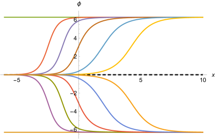
where $\varepsilon_{c}=\textrm{sgn}(c)$. Thus the solution represents a kink/antikink for positive/negative $c$, respectively. Depending on the inhomogeneity, however, the shape of the solution can be very different from the usual (anti)kink as we will see below. Changing the constant $c$ corresponds to changing the location of the (anti)kink as in the homogeneous theory. Recalling that there is no translation symmetry in the system, it is intriguing that there is still a position-like modulus parameter even for any inhomogeneous function $m(x)$. It is also worthwhile to note that all solutions asymptote to $\phi=0$ as $x\rightarrow-\infty$. As $x$ increases from the left, $\phi$ either goes up or goes down depending on the sign of $c$. In other words, there is no (anti)kink starting at $\phi=\frac{2\pi}{\beta}$. These are missing in the supersymmetric solutions of the theory since half of supersymmetry is broken here compared to the homogeneous theory.

In Fig. 1(a), we illustrate the solutions with

$$m(x)=\frac{1}{2}(m_{R}+m_{L})+\frac{1}{2}(m_{R}-m_{L})\tanh ax,\qquad(a>0).$$ (3.42)

In the figure, we set $m_{L}=2>m_{R}=1$ so that the vacuum solution is $\phi(x)=0$. We can clearly see that all kinks and antikinks start at $\phi=0$ for $x=-\infty$. Note that the width of the (anti)kink solutions in the left side is thinner than that in the right side.

The energy of the solution (3.39) denoted by $E_{\textrm{nc}}$ is given by

$$E_{\textrm{nc}} =m(\infty)W_{0}(\phi(\infty))-m(-\infty)W_{0}(\phi(-\infty))$$

$$=\frac{4}{\beta^{2}}(|m_{L}|+|m_{R}|),$$ (3.43)

which is positive and independent of the integration constant $c$ as it should be. In this expression, we take absolute values of $m_{L}$ and $m_{R}$ which are redundant in this case but turn out to be needed in other cases as seen below.

If both $m_{L}$ and $m_{R}$ are negative, the Bogomolny equation reduces to the previous case by the simple parity operation $x\rightarrow-x$. Then the solution will be an antikink/kink for positive/negative $c$, but now the solution starts at $\phi(-\infty)=\varepsilon_{c}\frac{2\pi}{\beta}$ and goes to zero as $x\rightarrow\infty$. The energy $E_{\textrm{nc}}$ would again be given by (3).

When the signs of $m_{L}$ and $m_{R}$ are different from each other, the solutions belong to a different topological sector because $\mu(x)$ in (3.40) goes asymptotically to the same values at both spatial infinities. If $m_{L}<0$ and $m_{R}>0$, $e^{\mu(x)}\rightarrow\infty$ as $x\rightarrow\pm\infty$ and hence

$$\phi(x)\rightarrow\varepsilon_{c}\frac{2\pi}{\beta},\qquad x\rightarrow\pm\infty.$$ (3.44)

The energy $E_{\textrm{nc}}$ of the solution is again given by (3). Finally, in the case that $m_{L}>0$ and $m_{R}<0$, we have

$$\phi(x)\rightarrow 0,\qquad x\rightarrow\pm\infty,$$ (3.45)

with the same energy expression (3). Note that in these two cases, $\phi(x)$ asymptotes to the constant solution which is not the vacuum.

(a)

(b)

Figure 1: Supersymmetric solutions of deformed SSG theory for $m(x)$ in (3.42) with $\beta=a=1$. (a) $m_{L}=2$ and $m_{R}=1$. The vacuum is the dashed straight line $\phi=0$ (mod $4\pi$) with energy $E=-4$. The other constant solution $\phi=2\pi$ (mod $4\pi$) has energy $E=4$. Non-constant (anti)kink-like solutions are for $c=100,\ 10,\ 1,\ 0.1,\ 0.01,\ -0.01,\ -0.1,\ -1,\ -10$, and $-100$, respectively from the top. They all have energy $E_{\textrm{nc}}=2$. (b) $m_{L}=-1$ and $m_{R}=2$. The vacuum is the dashed straight line $\phi=0$ (mod $4\pi$) with energy $E=-12$. The other constant solution $\phi=2\pi$ (mod $4\pi$) has energy $E=12$. Nonconstant solutions are for $c=10,\ 1,\ 0.1,\ 0.01,\ -0.01,\ -0.1,\ -1$ and $-10$, respectively from the top. They all have energy $E_{\textrm{nc}}=12$.

Combining with the energies for constant solutions (3.35), we have a rather rich BPS energy spectrum of supersymmetric solutions which depends on the asymptotic values of $m(x)$. If $m_{R}=m_{L}\equiv m_{0}$, all constant configurations (3.32) are degenerate with vanishing energy. There are also non-constant solutions which interpolate between two adjacent constant values of $\phi_{n}$ in (3.32) with energy $E_{\textrm{nc}}=\frac{8}{\beta^{2}}|m_{0}|$. In the homogeneous case that $m(x)=m_{0}$ everywhere, these are nothing but the kink and the antikink solutions with $\mu=m_{0}x$ in (3.39). In the present case, however, there are two differences from the usual homogeneous case: half of the (anti)kink is missing as explained above, and the shape of the solutions can be very complicated in general, depending on the functional form of $m(x)$. Nevertheless, the energy does not change under arbitrary inhomogeneous deformations but is solely determined by the asymptotic values of $m(x)$.

If $m_{R}\neq m_{L}$, we have two energy levels $E_{\textrm{vac}}$ and $E_{1}=|E_{\textrm{vac}}|$ for constant solutions (3.32), as described above. In addition, we have non-constant solutions with energy $E_{\textrm{nc}}$ in (3). For the case that $m_{L}$ and $m_{R}$ have the same sign, $E_{\textrm{nc}}$ is higher than those of constant solutions. Thus we have three discrete energy levels for supersymmetric solutions

$$E_{\textrm{vac}}<0<E_{1}=|E_{\textrm{vac}}|<E_{\textrm{nc}}.$$ (3.46)

On the other hand, if the signs of $m_{L}$ and $m_{R}$ are different, the energy $E_{\textrm{nc}}$ of non-constant solutions obtained in (3) is the same as $E_{1}$. In other words, they become degenerate and we have only two energy levels,

$$E_{\textrm{vac}}<0<E_{1}=|E_{\textrm{vac}}|=E_{\textrm{nc}}.$$ (3.47)

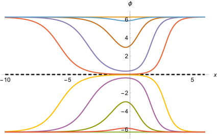
In fact, the constant solution $\phi(x)=\phi_{2n+1-\delta}$ is a special limit of the non-constant solution (3.39) obtained by taking either $c=0$ or $c=\infty$ limit. So they form a continuously deformable one-parameter family of degenerate solutions where the constant solution lies in the middle of the family. Note that there is no (anti)kink-like solutions in this case. Also the integration constant $c$ is no longer directly interpreted as position of the solution. It determines the height of the solution rather than the location. For sufficiently large $c$, however, the solution may be interpreted as a threshold bound state of a kink-antikink pair and then $c$ would determine the separation distance of them. This can be seen in Fig. 1(b) where solutions are depicted for $m_{L}=-1$ and $m_{R}=2$. In the figure, when $|c|\ll 1$, we can clearly identify a kink-antikink pair in the solution. As $|c|$ increases the kink and the antikink start loosing their identity and eventually become the non-vacuum constant configuration. It should be noted that these are all static supersymmetric configurations, in contrast to the standard sine-Gordon theory where the kink-antikink pair, or the breather solution is time-dependent. Of course, in the inhomogeneous theory this is possible due to the extra term $\frac{\partial W}{\partial x}$ in the potential so that the interaction between the kink and the antikink is cancelled out.

We would like to note that, of the two constant solutions, there is no further solution around the true vacuum, while there are more solutions around the non-vacuum constant solution when $m_{L}\,m_{R}<0$ and they together form a continuously deformable family of degenerate solutions. This is not just a specific feature of the sine-Gordon theory. Indeed, the same phenomenon occurs also in the deformed $\phi^{4}$ theory which is briefly discussed in the Appendix. Moreover, as we see in the next section, there is a similar phenomenon in $\phi^{6}$ theory where the vacuum expectation value is inhomogeneously deformed, which is completely different from the inhomogeneity discussed here. Apparently, this comes from the fact that the energy of static supersymmetric solutions depends only on the boundary values of the superpotential. Thus if there are any non-constant solutions with the same boundary values as those of a constant solution, they must be energetically degenerate. Since non-constant solutions should have a free parameter as argued above, it could potentially be connected to the constant solution, although not always guaranteed to be so. It would be interesting to figure out what class of inhomogeneous theories would have this feature.

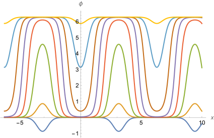
For different choice of $m(x)$, the profile of solutions can be arbitrarily complicated. The (anti)kink solution or kink-antikink pair solution described above can actually consist of many kinks and antikinks. As a simple illustration, we depict the solution for

$$m(x)=5\sin x$$ (3.48)

with $\beta=1$ for various integration constant $c$ in Fig. 2. Since it is periodic, it forms an infinite array of kink-antikink pairs. Furthermore, it is smoothly deformed to constant solutions $\phi=0$ or $\phi=2\pi$, as $c$ goes to $0$ or $\infty$. The periodic inhomogeneous deformation would be relevant when the system is put in a circle. This example demonstrates that, in this case, there is no longer a potential barrier between the constant solutions in the space of solutions. Thus there is a flat direction at the minima of the potential in the space of solutions and they are connected by one-parameter family of supersymmetric solutions. The same phenomenon would happen in other inhomogeneous theories.

Figure 2: Supersymmetric solutions of deformed SSG theory for $m(x)=5\sin x$ with $\beta=1$. From the top, $c=10,\ 1,\ 0.1,\ 10^{-2},\ 10^{-3},\ 10^{-4}$, and $-10^{-4}$, respectively.

We conclude this section by considering the sharp interface limit for the mass function (3.42). If $a\rightarrow\infty$, it reduces to

$$m(x)=m_{L}\theta(-x)+m_{R}\theta(x),$$ (3.49)

and the potential (3.30) becomes

$$V=\theta(-x)2\frac{m_{L}^{2}}{\beta^{2}}\sin^{2}\frac{\beta\phi}{2}+\theta(x)2\frac{m_{R}^{2}}{\beta^{2}}\sin^{2}\frac{\beta\phi}{2}-\delta(x)\frac{4(m_{R}-m_{L})}{\beta^{2}}\cos\frac{\beta\phi}{2}.$$ (3.50)

Then the last term of the potential proportional to the delta function is a pointlike impurity at the origin. Since the original potential depends only on the squares of the masses, there are four possibilities in the impurity strength for given $m_{L}^{2}$ and $m_{R}^{2}$, i.e., $m_{L}-m_{R}$ can be identified as $\pm(|m_{L}|+|m_{R}|)$ or $\pm(|m_{L}|-|m_{R}|)$ depending on the signs of $m_{L}$ and $m_{R}$. The resulting quantum theory could be further studied using various techniques in quantum field theory, which is beyond the scope of this paper.

4 Inhomogeneous Deformation of the Vacuum Expectation Value in $\phi^{6}$ Theory

Let us consider a quartic superpotential,

$$\frac{\lambda}{4}(\phi^{4}-2w\phi^{2}).$$ (4.51)

If the parameters $\lambda$ and $w$ are constants, it results in the sextic potential

$$\frac{\lambda^{2}}{2}\phi^{2}(\phi^{2}-w)^{2}.$$ (4.52)

For a positive $w$, this potential is triply degenerate with vacua at $\phi=0,\pm\sqrt{w}$. On the other hand, for negative $w$, there is only one vacuum at the origin $\phi=0$. If $\lambda$ is dependent on the position, we would get similar results to the previous section. Here, we let $w$ be inhomogeneous instead,

$$W(\phi,x)=\frac{\lambda}{4}[\phi^{4}-2w(x)\phi^{2}],$$ (4.53)

so that the corresponding potential (2.14) becomes

$$V(\phi,x)=\frac{\lambda^{2}}{2}\phi^{2}(\phi^{2}-w(x))^{2}-\frac{\lambda}{2}w^{\prime}(x)\phi^{2}.$$ (4.54)

Figure 3: An example of the inhomogeneous potential $V(\phi,x)$ in (4.54) with $w(x)=\tanh x$ and $v=\lambda=1$.

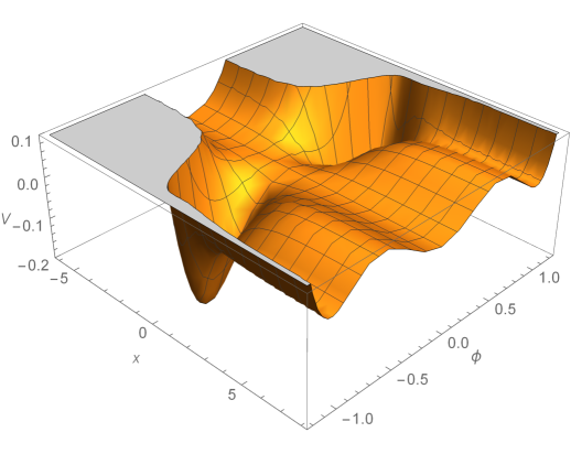
We illustrate the shape of the potential in Fig. 3 for $w(x)=\tanh x$ and $\lambda=v=1$.

It is important to note the difference from the overall rescaling considered in the previous section. In the present case, the minima of the potential (4.54) depend on the position and even the total number of the minima can change as shown in Fig. 3, since $w$ may not be positive definite. One may think that half of the system lies in some different physical situation such as external field, or two heterogeneous systems with distinct potentials smoothly joined together while supersymmetry is preserved. Then the vacuum need not just be given by a constant configuration in general, in contrast with the previous case where the vacuum configurations are constants since the overall shape of the superpotential is not deformed.

Supersymmetric solutions satisfy the Bogomolny equation

$$\phi^{\prime}(x)-\lambda\phi(x)[\phi^{2}(x)-w(x)]=0.$$ (4.55)

We assume that $w(x)$ goes to some finite values $w_{L/R}$ as $x\rightarrow\pm\infty$ which are not necessarily positive. Then possible asymptotic values of $\phi(x)$ depend on the signs of $w_{L}$ and $w_{R}$. If both $w_{L}$ and $w_{R}$ are negative, $\phi(x)$ should vanish at spatial infinities to achieve the minimum energy. If one or both of $w_{L}$ and $w_{R}$ are positive, $\phi$ can go to $\pm\sqrt{w_{L}}$ or $\pm\sqrt{w_{R}}$ at spatial infinities. The superpotential at these values are

$$W(0) =0,$$

$$W(\pm\sqrt{w_{R}}) =-\frac{\lambda}{4}w_{R}^{2},$$

$$W(\pm\sqrt{w_{L}}) =-\frac{\lambda}{4}w_{L}^{2}.$$ (4.56)

Now let us solve the Bogomolny equation (4.55). An obvious solution is

$$\phi(x)=0,$$ (4.57)

of which the energy vanishes. This constant solution is possible since $\phi(x)=0$ is still an extremum of the potential irrespective of the function $w(x)$. There exist other solutions. In fact, the Bogomolny equation (4.55) is integrable for arbitrary $w(x)$. The general solution is given by

$$\phi^{2}(x)=\frac{e^{-2\lambda\Omega(x)}}{2\lambda(c-\xi(x))},$$ (4.58)

where $c$ is an integration constant and

$$\Omega(x) =\int w(x)dx,$$

$$\xi(x) =\int e^{-2\lambda\Omega(x)}dx.$$ (4.59)

Then $\Omega(x)\sim w_{R/L}x$ as $x\rightarrow\pm\infty$. Since $\phi^{2}(x)$ is positive, $\xi(x)$ in the denominator of (4.58) should be bounded from above by the integration constant $c$. From (4), $\xi(x)$ is monotonically increasing and then the asymptotic values of $w(x)$ is restricted to be $w_{R}\geq 0$ for the solution not to be divergent, while $w_{L}$ can take any value.

The energy of the solution is calculated from the asymptotic values of $\phi(x)$ at spatial infinities $x\rightarrow\pm\infty$. Since the theory is symmetric under the sign flip $\phi\rightarrow-\phi$, it is enough to take into account $\phi(\infty)\geq 0$ case only. Let us first consider $x\rightarrow-\infty$ limit in which $\phi(-\infty)$ is determined by $w_{L}$. If $w_{L}>0$, both the numerator and the denominator of (4.58) diverges and the limit can be calculated with the help of L’Hôpital’s rule,

$$\phi^{2}(x)\xrightarrow{x\rightarrow-\infty}\frac{-2\lambda w(x)e^{-2\lambda\Omega(x)}}{-2\lambda e^{-2\lambda\Omega(x)}}\longrightarrow w_{L}.$$ (4.60)

For $w_{L}\leq 0$, it is easy to see that the numerator of (4.58) vanishes while the denominator does not in $x\rightarrow-\infty$ limit, i.e., $\phi(-\infty)=0$.

Next, we consider $x\rightarrow\infty$ limit. From (4.58), we see that $\phi(\infty)$ depends on the value of the denominator. If $\xi(\infty)$ is strictly less than $c$, $\phi^{2}(x)\sim e^{-2\lambda w_{R}x}$ as $x\rightarrow\infty$ and hence the solution vanishes $x\rightarrow\infty$. If $\xi(\infty)=c$, the denominator in (4.58) vanishes asymptotically. In this case, the solution (4.58) may be written in a more explicit form by absorbing the integration constant $c$ as

$$\phi^{2}(x)=\frac{e^{-2\lambda\Omega(x)}}{2\lambda\int_{x}^{\infty}e^{-2\lambda\Omega(x^{\prime})}dx^{\prime}}.$$ (4.61)

In $x\rightarrow\infty$ limit, we again use L’Hôpital’s rule to get $\phi^{2}(\infty)=w_{R}$. In other words, $\phi(\infty)$ vanishes for all integration constant $c$ except one specific value for which $\phi(\infty)=\sqrt{w_{R}}$. It is amusing to see how the solution with different boundary condition arises naturally for a special value of the integration constant.

We have now four different asymptotic values at spatial infinities, depending on the integration constant and the sign of $w_{L}$. For each case, the corresponding energy can be calculated as the difference of the superpotential as in Table 1.

$w_{L}$	$c$	$\phi^{2}(-\infty)$	$\phi^{2}(\infty)$	$E$
$w_{L}>0$	$c>\xi(\infty)$	$w_{L}$	0	$\frac{\lambda}{4}w_{L}^{2}$
	$c=\xi(\infty)$	$w_{L}$	$w_{R}$	$\frac{\lambda}{4}(w_{L}^{2}-w_{R}^{2})$
$w_{L}\leq 0$	$c>\xi(\infty)$	0	0	0
	$c=\xi(\infty)$	0	$w_{R}$	$-\frac{\lambda}{4}w_{R}^{2}$

Table 1: Asymptotic values and energies of the non-constant solution (4.58) in deformed $\phi^{6}$ theory. In addition, there is a constant solution $\phi=0$ with $E=0$.

Let us now summarize the supersymmetric solutions of the theory. There is always a trivial solution $\phi(x)=0$ with vanishing energy. If $w_{L}>0$, we have a unique solution (4.61) interpolating between $\phi(-\infty)=\sqrt{w_{L}}$ and $\phi(\infty)=\sqrt{w_{R}}$. The energy of these solutions is $E=\frac{\lambda}{4}(w_{L}^{2}-w_{R}^{2})$ which can either be positive or negative depending on the value of $w_{L}$ and $w_{R}$. If $w_{L}<w_{R}$, the energy becomes lower than that of the trivial $\phi=0$ solution and we have two degenerate vacua (including the sign-flipped solution) with negative energy. If $w_{L}=w_{R}$ we would have triply degenerate vacua with vanishing energy. There are also a one-parameter family of degenerate solutions with higher energy $E=\frac{\lambda}{4}w_{L}^{2}$.

If $w_{L}\leq 0$, we have again a unique solution (4.61) which now interpolates between $\phi(-\infty)=0$ and $\phi(\infty)=\sqrt{w_{R}}$ with negative energy $E=-\frac{1}{4}\lambda w_{R}^{2}$. All the other solutions have vanishing energy irrespective of the value of $c$, since the energy depends only on the boundary values of $\phi$. They form a one-parameter family of degenerate solutions which includes the constant solution $\phi(x)=0$ as a special $c\rightarrow 0$ limit, similar to what we have seen in the previous section.

Note that, even though we have a constant solution $\phi(x)=0$ with vanishing energy, this is not the vacuum solution of minimum energy except $w_{L}>w_{R}$ case. The true vacuum is not constant but interpolates between two different values of the minima with negative energy: either $\phi(-\infty)=\sqrt{w_{L}}$ and $\phi(\infty)=\sqrt{v_{R}}$ (for $w_{R}>w_{L}\geq 0$), or $\phi(-\infty)=0$ and $\phi(\infty)=\sqrt{w_{R}}$ (for $w_{L}<0<w_{R}$).

As an explicit example, let us consider a specific spatial dependence as before,

$$w(x)=\frac{1}{2}(w_{R}+w_{L})+\frac{1}{2}(w_{R}-w_{L})\tanh ax,\qquad(a>0).$$ (4.62)

Then we can express the solution (4.58) in terms of a hypergeometric function which is rather complicated and it is not much illuminating to show it here. Instead, we choose some simple $w_{L}$’s for fixed $w_{R}$ and see explicitly how the solution changes as we vary $w_{L}$.

• If $w_{L}=w_{R}$, $w(x)$ is constant and we have a usual homogeneous $\phi^{6}$ theory. Then the solution reduces to [39]

  $$\phi(x)=\pm\left(\frac{w_{R}}{1+c\,e^{2\lambda w_{R}x}}\right)^{1/2},$$ (4.63)

  which are antikink/kink solutions interpolating between $\phi(-\infty)=\pm\sqrt{w_{L}}$ respectively, and $\phi(\infty)=0$ if $c>0$. When $c=0$, the solutions become constant solutions $\phi(x)=\pm\sqrt{w_{R}}$ which are just the vacua degenerate with $\phi(x)=0$ configuration. Note that, in homogeneous case, the supersymmetry is enhanced and we have other supersymmetric solutions which are kinks/antikinks interpolating 0 and $\pm\sqrt{w_{R}}$, respectively. They are, however, not solutions of (4.55) but solutions of the equation with positive sign in front of $\lambda$ in (4.55).

• If $w_{L}=2w_{R}$ and $a=\lambda w_{R}$, the solution is expressed in terms of elementary functions,

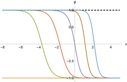
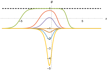
  $$\phi(x)=\pm\left(\frac{2w_{R}(1+e^{2\lambda w_{R}x})}{1+2e^{2\lambda w_{R}x}+c\,e^{4\lambda w_{R}x}}\right)^{1/2},$$ (4.64)

  which interpolates between $\pm\sqrt{w_{L}}(=\pm\sqrt{2w_{R}})$ and 0 for $c>0$, respectively, and $\pm\sqrt{w_{L}}$ and $\pm\sqrt{w_{R}}$ for $c=0$, respectively. Since $w_{L}>w_{R}$, these solutions have positive energies and the vacuum solution is $\phi(x)=0$. We draw the solutions for various $c$ in Fig. 4 with $a=\lambda=w_{R}=1$. The vacuum solution is depicted with a dashed line. For large $c$, the (anti)kink lies in the left side. As $c$ gets smaller, it moves to the right side but the height of the solution changes to $\sqrt{w_{R}}$ so that it looks like double (anti)kinks separated with the left (anti)kink being fixed around $x=0$. When $c=0$, the boundary value at $x=\infty$ changes from $\phi=0$ to $\phi=\pm\sqrt{w_{R}}$ which reduces the energy from $E=\lambda w_{R}^{2}$ to $E=\frac{3}{4}w_{R}^{2}$.

  

  

  

  

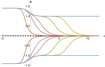
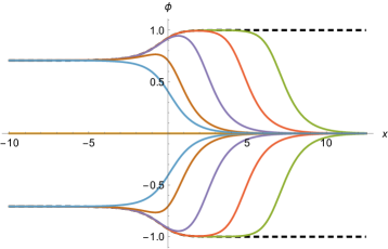
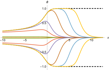
  Figure 4: Supersymmetric solutions of the deformed $\phi^{6}$ theory for $w(x)$ given in (4.62) with $a=\lambda=w_{R}=1$. Solutions in $\phi<0$ region are obtained by $\phi\rightarrow-\phi$. In each figure, vacuum solutions are depicted with dashed lines. (a) Plots for $w_{L}=2$. The topmost curve interpolates between $\sqrt{2}$ and 1 and has energy $E=\frac{3}{4}$. The other solutions interpolating between $\sqrt{2}$ and 0 are for $c=100,\ 1,\ 0.1,\ 10^{-3}$, and $10^{-5}$, respectively from the left. The energy of these solutions are all $E=1$. (b) Plots for $w_{L}=\frac{1}{2}$. The dashed curves interpolating between $\pm\frac{1}{\sqrt{2}}$ and 1 are vacuum solutions with negative energy $E=-\frac{3}{16}$. The other solutions interpolating between $\frac{1}{\sqrt{2}}$ and 0 are for $c=1,\ -1,\ -\sqrt{2}+10^{-2},\ -\sqrt{2}+10^{-4}$, and $-\sqrt{2}+10^{-6}$, respectively from the left. The energy of these solutions are all $E=\frac{1}{16}$. (c) Plots for $w_{L}=0$. The dashed curves interpolating between 0 and $\pm 1$ are vacuum solutions with negative energy $E=-\frac{1}{4}$. The other solutions all vanish as $x\rightarrow\pm\infty$ and are for $c=10^{-6},\ 10^{-4},\ 10^{-2},\ 1,\ 10,\ 10^{3}$ and $\infty$, respectively from the top. The energy of these solutions are all zero. (d) Plots for $w_{L}=-1$. The vacuum solutions are dashed curves interpolating between 0 and $\pm 1$ with energy $E=-\frac{1}{4}$. The other solutions vanishing at both spatial infinities are for $c=1.0001,\ 1.1,\ 2,\ 10$, and $\infty$, respectively from the top. The energies of these solutions are all zero.

• If $w_{L}=\frac{w_{R}}{2}$ and $a=\lambda w_{R}$, we have

  $$\phi(x)=\pm\left(\frac{w_{R}}{2}\frac{1}{1+e^{2\lambda w_{R}x}+c\,e^{3\lambda w_{R}x/2}\sqrt{\cosh\lambda w_{R}x}}\right)^{1/2},$$ (4.65)

  where $c>-\sqrt{2}$ corresponds to the solution interpolating between $\pm\sqrt{w_{L}}(=\pm\sqrt{\frac{w_{R}}{2}})$ and 0 with energy $E=\frac{\lambda}{4}w_{L}^{2}=\frac{\lambda}{16}w_{R}^{2}$, while $c=-\sqrt{2}$ gives the vacuum solutions interpolating between $\pm\sqrt{w_{L}}$ and $\pm\sqrt{w_{R}}$, respectively, with negative energy $\frac{\lambda}{4}(w_{L}^{2}-w_{R}^{2})=-\frac{3\lambda}{16}w_{R}^{2}$. We draw the solutions in Fig. 4 with $a=\lambda=w_{R}=1$ where the dashed lines represent the vacuum solutions which are no longer constants.

• If $w_{L}=0$ and $a=\lambda w_{R}$, the solution becomes

  $$\phi(x)=\pm\left(\frac{w_{R}}{2}\frac{1-\tanh\lambda w_{R}x}{c+\ln(1+e^{-2\lambda w_{R}x})}\right)^{1/2}.$$ (4.66)

  For $c>0$, the solutions vanish at both spatial infinities and hence have vanishing energy. The constant solution $\phi(x)=0$ is obtained in $c\rightarrow\infty$ limit. For $c=0$, they interpolate between 0 and $\pm\sqrt{w_{R}}$ with negative energy $E=-\frac{\lambda}{4}w_{R}^{2}$ and hence they are the vacuum solutions. Note that, with this form of $w(x)$, the potential smoothly interpolates between the unbroken phase with pure $\phi^{6}$ potential in the left side of the space and the broken phase with three degenerate minima at 0 and $\pm\sqrt{w_{R}}$ in the right side of the space, while keeping the supersymmetry. We draw the solutions in Fig. 4 with $a=\lambda=w_{R}=1$. The vacuum solutions are depicted with dashed lines.

• Finally, we consider the case $w_{L}=-w_{R}<0$ and $a=\lambda w_{R}$, for which $w(x)$ is simply given by

  $$w(x)=w_{R}\tanh\lambda w_{R}x.$$ (4.67)

  Then in the left half of space the sextic potential has only one minimum at the origin $\phi=0$, while, in the right half, it has three minima at $\phi=0$ and $\pm\sqrt{w_{R}}$. Now the solution (4.58) becomes

  $$\phi(x)=\pm\left(\frac{w_{R}}{2}\frac{\operatorname{sech}^{2}\lambda w_{R}x}{c-\tanh\lambda w_{R}x}\right)^{1/2},$$ (4.68)

  which requires $c\geq 1$. If $c>1$, these solutions vanish at both spatial infinities and the corresponding energy is zero. The solutions with different $c$ are all degenerate and the constant solution $\phi(x)=0$ is obtained in $c\rightarrow\infty$ limit. If $c=1$, (4.68) reduces to

  $$\phi(x)=\pm\left[\frac{w_{R}}{2}(1+\tanh\lambda w_{R}x)\right]^{1/2},$$ (4.69)

  which interpolates between 0 and $\pm\sqrt{w_{R}}$, respectively, with energy $E=-\frac{1}{4}\lambda w_{R}^{2}$. Note that the shape of (4.69) is identical to the kink/antikink solutions in the homogeneous theory which are given in (4.63) with $c=1$ and $x\rightarrow-x$. In our case, however, these configurations are the vacuum solutions with negative energy. The solutions are depicted in Fig. 4 with $a=\lambda=w_{R}=1$. As we seen in this case and also in the $w_{L}=0$ case discussed above, the constant solution $\phi(x)=0$ and non-constant solutions around it which have the same boundary values form a continuously deformable one-parameter family of degenerate solutions, a phenomenon seen in the previous section.

5 Discussions

We studied inhomogeneous supersymmetric field theories classically in two dimensions where the superpotential depends explicitly on the spatial coordinate. Though the translational invariance is broken, half of the supersymmetry can be preserved by adding a term in the Lagrangian which is simply given by the spatial derivative of the superpotential. Analyzing the superalgebra, we showed that the energy is bounded from below by a topological charge which is not necessarily nonnegative definite. The energy bound is saturated for supersymmetric configurations satisfying the first-order Bogomolny equation.

There would be, in principle, many different types of inhomogeneity. In this paper, we considered two types of inhomogeneity: One is the inhomogeneous rescaling of the superpotential for SSG theory and the other is inhomogeneous deformation of the vacuum expectation value in $\phi^{6}$ theory. For these theories, we obtained the most general solutions of the Bogomolny equation and their energies which depend only on the boundary values of the superpotential. There is in general a zero mode around the non-vacuum solution which persists even under any arbitrary inhomogeneous deformation. Since the deformation function is arbitrary, one can consider various specific forms to obtain interesting physical situations such as sharp interface limit, or periodic functions.

In this paper, we considered only supersymmetric solutions of three classical theories in two dimensions. It would be interesting to investigate dynamical as well as quantum aspects of the theories in detail including zero mode dynamics and higher excitations. The structure of the solution space could be much richer in inhomogeneous theories as we have seen in this paper. In addition, we may consider other kind of inhomogeneities not studied in this paper. An immediate possibility would be to perform deformations of both the rescaling and the vacuum expectation value at the same time for theories considered here or for other theories. One may also deform other parameters not considered here. Another possibility is to deform the form of the potential by adding new terms. In this direction, impurities were studied in [20] by adding new terms to the original Lagrangian as in (2.24). Also the kinetic term can have inhomogeneity as seen in (2.21).

Since the superpotential $W$ is arbitrary in our formulation, one can consider inhomogeneous deformations of any existing homogeneous theories other than those studied here. For example, double SG model [40, 41] and models with higher-order polynomial potentials [42, 43] would be natural candidates to extend the results of SG theory and $\phi^{6}$ theory, respectively.

More generally, one may imagine two or more heterogeneous systems smoothly joined together with half of the supersymmetry being kept. The $\phi^{6}$ theory in section 4 can be considered as a simple example of this kind since it connects two potentials with different vacuum structures. In this case, the vacuum configuration would be no longer constant in general.

It should not be difficult to consider higher-dimensional theories with more field contents such as gauge fields. In fact, as mentioned in the introduction, there are already many studies on inhomogeneous supersymmetric field theories in various dimensions. However, we believe that the consequences of the inhomogeneity have not been fully explored. We will investigate these issues in separate publications [44].

Appendix A $\phi^{4}$ theory

In this appendix, we consider inhomogeneous rescaling of $\phi^{4}$ theory with a double-well potential. It has already been investigated in [23, 24]. Since it is a prototypical example, however, we summarize the results and discuss energy spectrum which differs from [23] because the definition of the energy is not the same as discussed in section 2. The deformed potential reads

$$V(\phi,x)=\frac{1}{2}g^{2}(x)(\phi^{2}-v^{2})^{2}+\frac{1}{3}g^{\prime}(x)(\phi^{3}-3v^{2}\phi),$$ (A.70)

which corresponds to the superpotential $W_{0}$ given by

$$W_{0}=\int(\phi^{2}-v^{2})d\phi=\frac{1}{3}\phi^{3}-v^{2}\phi.$$ (A.71)

Here we have dropped the trivial field-independent term as discussed in section 2. $W_{0}$ involves two extrema $\phi=\pm v$ which trivially satisfy the Bogomolny equation (3.28) and have the values

$$W_{0}(\pm v)=\mp\frac{2}{3}v^{3}.$$ (A.72)

The corresponding energies are

$$E_{\phi=\pm v}=\mp\frac{2}{3}v^{3}(g_{R}-g_{L}).$$ (A.73)

The vacuum energy is then the minimum of the two,

$$E_{\textrm{vac}}=-\frac{2}{3}v^{3}|g_{R}-g_{L}|,$$ (A.74)

which is negative unless $g_{L}=g_{R}$.

Depending on the magnitude of $\phi(x)$, there are two types [23] of nontrivial solutions of the Bogomolny equation (3.28). The first type is given by

$$\phi(x)=-v\tanh(vG(x)-c),$$ (A.75)

which satisfies $|\phi(x)|<v$. Here $c$ is an integration constant and

$$G(x)=\int_{0}^{x}g(x^{\prime})dx^{\prime}.$$ (A.76)

For the other type, $|\phi(x)|>v$ and the solution is

$$\phi(x)=-v\coth(vG(x)-c).$$ (A.77)

The energy of the solutions may be obtained from the asymptotic behavior of $G(x)$,

$$G(x)\rightarrow g_{R/L}x+\cdots,\qquad x\rightarrow\pm\infty.$$ (A.78)

Then the solutions (A.75) and (A.77) behave asymptotically as

$$\phi(x)\rightarrow\begin{cases}\textrm{sgn}(g_{L})v,\qquad x\rightarrow-\infty,\\ -\textrm{sgn}(g_{R})v,\qquad x\rightarrow\infty,\end{cases}$$ (A.79)

and hence the corresponding energy denoted by $E_{\textrm{nc}}$ is computed to be

$$E_{\textrm{nc}} =g(\infty)W_{0}(\phi(\infty))-g(-\infty)W_{0}(\phi(-\infty))$$

$$=\frac{2}{3}v^{3}(|g_{R}|+|g_{L}|),$$ (A.80)

which is independent of the integration constant $c$.

As in the SSG case, we have different types of solutions and energy levels depending on the asymptotic values of $g(x)$. If $g_{L}\,g_{R}>0$, the non-constant solutions are basically deformed kinks or antikinks interpolating between two values $\phi=v$ and $\phi=-v$. Unlike the SSG case, however, here we have only one type of solutions either kinks or antikinks but not both. Also there is no coth-type solution in this case. Since the energy $E_{\textrm{nc}}$ of non-constant solutions are higher than those of constant solutions, we have three discrete energy levels for supersymmetric solutions,

$$E_{\textrm{vac}}=E_{\phi=\varepsilon v}<0<E_{\phi=-\varepsilon v}<E_{\textrm{nc}},$$ (A.81)

where $\varepsilon\equiv\textrm{sgn}(g_{R}-g_{L})$. If the signs of $g_{L}$ and $g_{R}$ are different, $\phi\rightarrow-\varepsilon v$ at both spatial infinities, which is not the vacuum value, and the corresponding energy $E_{\textrm{nc}}$ in (A) becomes identical to $E_{\phi=-\varepsilon v}$. Therefore we have only two energy levels for supersymmetric solutions,

$$E_{\textrm{vac}}=E_{\phi=\varepsilon v}<0<E_{\phi=-\varepsilon v}=E_{\textrm{nc}}.$$ (A.82)

As in the SSG case, the non-constant solutions (A.75) and (A.77), and the non-vacuum constant solution $\phi(x)=-\varepsilon v$ form a continuously deformable one-parameter family of degenerate solutions obtained by changing the integration constant $c$.

These solutions are illustrated in Fig. 5 for the inhomogeneous scaling function

$$g(x)=\frac{1}{2}(g_{R}+g_{L})+\frac{1}{2}(g_{R}-g_{L})\tanh ax,\qquad(a>0).$$ (A.83)

Note that, compared with the SSG case, we have only antikinks in Fig. 5(a). Also the coth-type solution can indefinitely be negative in Fig. 5(b), which has also been discussed in [23].

(a)

(b)

Figure 5: Supersymmetric solutions of deformed $\phi^{4}$ theory for $g(x)$ in (A.83) with $v=a=1$. (a) $g_{L}=1$ and $g_{R}=2$. The vacuum is the dashed straight line $\phi=1$ with energy $E=-2/3$. The other constant solution $\phi=-1$ has energy $E=2/3$. Non-constant solutions are for $c=-4,\ -2,\ 0,\ 2$ and 4, respectively from the left. They all have degenerate energy $E_{\textrm{nc}}=2$. (b) $g_{L}=-1$ and $g_{R}=2$. The vacuum is the dashed straight line $\phi=1$ with energy $E=-2$. The other constant solution $\phi=-1$ has energy $E=2$. Non-constant solutions are for $c=4,\ 1,\ 0$ in (A.75), and $c=-1,\ -0.6,\ -0.3$ in (A.77), respectively from the top. They all have degenerate energy $E_{\textrm{nc}}=2$.

References

- [1] D. Bak, M. Gutperle and S. Hirano, “A dilatonic deformation of AdS(5) and its field theory dual,” JHEP 0305 (2003) 072 [arXiv:hep-th/0304129].
- [2] A. Clark and A. Karch, “Super Janus,” JHEP 10, 094 (2005) [arXiv:hep-th/0506265 [hep-th]].
- [3] E. D’Hoker, J. Estes and M. Gutperle, “Interface Yang-Mills, supersymmetry, and Janus,” Nucl. Phys. B 753, 16-41 (2006) [arXiv:hep-th/0603013 [hep-th]].
- [4] E. D’Hoker, J. Estes and M. Gutperle, “Exact half-BPS Type IIB interface solutions. I. Local solution and supersymmetric Janus,” JHEP 06, 021 (2007) [arXiv:0705.0022 [hep-th]].
- [5] C. Kim, E. Koh and K. M. Lee, “Janus and Multifaced Supersymmetric Theories,” JHEP 06, 040 (2008) [arXiv:0802.2143 [hep-th]].
- [6] C. Kim, E. Koh and K. M. Lee, “Janus and Multifaced Supersymmetric Theories II,” Phys. Rev. D 79, 126013 (2009) [arXiv:0901.0506 [hep-th]].
- [7] D. Gaiotto and E. Witten, “Janus Configurations, Chern-Simons Couplings, And The theta-Angle in N=4 Super Yang-Mills Theory,” JHEP 06, 097 (2010) [arXiv:0804.2907 [hep-th]].
- [8] D. Gaiotto and E. Witten, “S-Duality of Boundary Conditions In N=4 Super Yang-Mills Theory,” Adv. Theor. Math. Phys. 13, no.3, 721-896 (2009) [arXiv:0807.3720 [hep-th]].
- [9] K. K. Kim and O. K. Kwon, “Janus ABJM Models with Mass Deformation,” JHEP 08, 082 (2018) [arXiv:1806.06963 [hep-th]].
- [10] K. K. Kim, Y. Kim, O. K. Kwon and C. Kim, “Aspects of Massive ABJM Models with Inhomogeneous Mass Parameters,” JHEP 12, 153 (2019) [arXiv:1910.05044 [hep-th]].
- [11] I. Arav, K. C. M. Cheung, J. P. Gauntlett, M. M. Roberts and C. Rosen, “Spatially modulated and supersymmetric mass deformations of = 4 SYM,” JHEP 11, 156 (2020) [arXiv:2007.15095 [hep-th]].
- [12] Y. Kim, O. K. Kwon and D. D. Tolla, “Super Yang-Mills Theories with Inhomogeneous Mass Deformations,” JHEP 12, 060 (2020) [arXiv:2008.00868 [hep-th]].
- [13] J. P. Gauntlett and C. Rosen, “Susy Q and spatially modulated deformations of ABJM theory,” JHEP 10, 066 (2018) [arXiv:1808.02488 [hep-th]].
- [14] I. Arav, J. P. Gauntlett, M. Roberts and C. Rosen, “Spatially modulated and supersymmetric deformations of ABJM theory,” JHEP 04, 099 (2019) [arXiv:1812.11159 [hep-th]].
- [15] B. Ahn, S. Hyun, K. K. Kim, O. K. Kwon and S. A. Park, “AdS Q-Soliton and Inhomogeneously mass-deformed ABJM Model,” JHEP 02, 132 (2020) [arXiv:1911.05783 [hep-th]].
- [16] S. Hyun, B. Ahn, K. K. Kim, O. K. Kwon and S. A. Park, “Thermodynamics of Inhomogeneously Mass-deformed ABJM Model and Pressure Anisotropy,” JHEP 02, 062 (2020) [arXiv:1912.00784 [hep-th]].
- [17] I. Arav, K. C. M. Cheung, J. P. Gauntlett, M. M. Roberts and C. Rosen, “Superconformal RG interfaces in holography,” JHEP 11, 168 (2020) [arXiv:2007.07891 [hep-th]].
- [18] A. Hook, S. Kachru and G. Torroba, “Supersymmetric Defect Models and Mirror Symmetry,” JHEP 11, 004 (2013) [arXiv:1308.4416 [hep-th]].
- [19] D. Tong and K. Wong, “Vortices and Impurities,” JHEP 01, 090 (2014) [arXiv:1309.2644 [hep-th]].
- [20] C. Adam, J. M. Queiruga and A. Wereszczynski, “BPS soliton-impurity models and supersymmetry,” JHEP 07, 164 (2019) [arXiv:1901.04501 [hep-th]].
- [21] C. Adam and A. Wereszczynski, “BPS property and its breaking in 1+1 dimensions,” Phys. Rev. D 98, no.11, 116001 (2018) [arXiv:1809.01667 [hep-th]].
- [22] C. Adam, T. Romanczukiewicz and A. Wereszczynski, “The model with the BPS preserving defect,” JHEP 03, 131 (2019) [arXiv:1812.04007 [hep-th]].
- [23] C. Adam, K. Oles, J. M. Queiruga, T. Romanczukiewicz and A. Wereszczynski, “Solvable self-dual impurity models,” JHEP 07, 150 (2019) [arXiv:1905.06080 [hep-th]].
- [24] N. S. Manton, K. Oleś and A. Wereszczyński, “Iterated kinks,” JHEP 10, 086 (2019) [arXiv:1908.05893 [hep-th]].
- [25] C. Adam, K. Oles, T. Romanczukiewicz and A. Wereszczynski, “Domain walls that do not get stuck on impurities,” [arXiv:1902.07227 [cond-mat.mes-hall]].
- [26] C. Adam, K. Oles, T. Romanczukiewicz and A. Wereszczynski, “Spectral Walls in Soliton Collisions,” Phys. Rev. Lett. 122, no.24, 241601 (2019) [arXiv:1903.12100 [hep-th]].
- [27] T. Inami, S. Odake and Y. Z. Zhang, “Supersymmetric extension of the Sine-Gordon theory with integrable boundary interactions,” Phys. Lett. B 359, 118-124 (1995) [arXiv:hep-th/9506157 [hep-th]].
- [28] R. I. Nepomechie, “The Boundary supersymmetric sine-Gordon model revisited,” Phys. Lett. B 509, 183-188 (2001) [arXiv:hep-th/0103029 [hep-th]].
- [29] J. F. Gomes, L. H. Ymai and A. H. Zimerman, “The Super MKDV and Sinh-Gordon hierarchy: Solitons and Backlund defects,” J. Phys. A 39, 7471-7483 (2006) [arXiv:hep-th/0601014 [hep-th]].
- [30] P. Bowcock, E. Corrigan and C. Zambon, “Classically integrable field theories with defects,” Int. J. Mod. Phys. A 19S2, 82-91 (2004) [arXiv:hep-th/0305022 [hep-th]].
- [31] J. F. Gomes, L. H. Ymai and A. H. Zimerman, “Integrablility of a Classical N = 2 Super Sinh-Gordon Model with Jump Defects,” JHEP 03, 001 (2008) [arXiv:0710.1391 [hep-th]].
- [32] J. Iliopoulos and B. Zumino, “Broken Supergauge Symmetry and Renormalization,” Nucl. Phys. B 76, 310 (1974).
- [33] E. Witten and D. I. Olive, “Supersymmetry Algebras That Include Topological Charges,” Phys. Lett. B 78, 97-101 (1978).
- [34] E. Witten, “Dynamical Breaking of Supersymmetry,” Nucl. Phys. B 188, 513 (1981)
- [35] M. K. Prasad and C. M. Sommerfield, “An Exact Classical Solution for the ’t Hooft Monopole and the Julia-Zee Dyon,” Phys. Rev. Lett. 35, 760-762 (1975)
- [36] E. B. Bogomolny, “Stability of Classical Solutions,” Sov. J. Nucl. Phys. 24, 449 (1976) PRINT-76-0543 (LANDAU-INST.).
- [37] P. Di Vecchia and S. Ferrara, “Classical Solutions in Two-Dimensional Supersymmetric Field Theories,” Nucl. Phys. B 130, 93-104 (1977).
- [38] J. Hruby, “On the Supersymmetric Sine-Gordon Model and a Two-Dimensional Bag,” Nucl. Phys. B 131, 275-284 (1977).
- [39] M. A. Lohe, “Soliton Structures in ,” Phys. Rev. D 20, 3120 (1979).
- [40] C. A. Condat, R. A. Guyer, and M. D. Miller, “Double Sine-Gordon Chain,” Phys. Rev. D 27, 474 (1983).
- [41] V. A. Gani, A. M. Marjaneh, A. Askari, E. Belendryasova and D. Saadatmand, “Scattering of the double sine-Gordon kinks,” Eur. Phys. J. C 78, no.4, 345 (2018) [arXiv:1711.01918 [hep-th]].
- [42] A. Khare, I. C. Christov and A. Saxena, “Successive phase transitions and kink solutions in , , and field theories,” Phys. Rev. E 90, no.2, 023208 (2014) [arXiv:1402.6766 [math-ph]].
- [43] I. C. Christov, R. J. Decker, A. Demirkaya, V. A. Gani, P. G. Kevrekidis and R. V. Radomskiy, “Long-range interactions of kinks,” Phys. Rev. D 99, no.1, 016010 (2019) [arXiv:1810.03590 [hep-th]].
- [44] C. Kim, Y. Kim, O-K. Kwon and H. Song, work in progress.