Event-triggered Consensus of Matrix-weighted Networks Subject to Actuator Saturation

Abstract

The ubiquitous interdependencies among higher-dimensional states of neighboring agents can be characterized by matrix-weighted networks. This paper examines event-triggered global consensus of matrix-weighted networks subject to actuator saturation. Specifically, a distributed dynamic event-triggered coordination strategy, whose design involves sampled state of agents, saturation constraint and auxiliary systems, is proposed for this category of generalized network to guarantee its global consensus. Under the proposed event-triggered coordination strategy, sufficient conditions are derived to guarantee the leaderless and leader-follower global consensus of the multi-agent systems on matrix-weighted networks, respectively. The Zeno phenomenon can be excluded for both cases under the proposed coordination strategy. It turns out that the spectral properties of matrix-valued weights are crucial in event-triggered mechanism design for matrix-weighted networks with actuator saturation constraint. Finally, simulations are provided to demonstrate the effectiveness of proposed event-triggered coordination strategy. This work provides a more general design framework compared with existing results that are only applicable to scalar-weighted networks.

1 Introduction

Consensus problem on matrix-weighted networks is becoming a recent concern since, as an immediate generalization of scalar-weighted networks, they naturally captures interdependencies among higher-dimensional states of neighboring agents in a multi-agent network [1, 2, 3, 4, 5, 6]. Actually, matrix-weighted networks arise in scenarios such as graph effective resistance based distributed control and estimation [7, 8], logical inter-dependency of multiple topics in opinion evolution [9], bearing-based formation control [10], array of coupled LC oscillators [11] as well as consensus and synchronization on matrix-weighted networks [3, 4].

In contrast to scalar-weighted networks, connectivity alone does not translate to achieving consensus on matrix-weighted networks, properties of weight matrices now play an important role in the characterization of consensus as well as the design of interaction protocols subject to physical constraints. In literatures, positive/negative definiteness/semi-definiteness weight matrices have been employed to provide consensus conditions [3, 12, 2, 4]. In the meantime, it is worth noting that the matrix-weighted network is a more general category of multi-agent networks, recent trends in this line of research seems to involve the constraints of physical systems encountered in real-world applications. For instance, beyond the first-order local dynamics, consensus conditions for second-order multi-agent system on matrix-weighted networks are provided [13, 14]. However, a comprehensive investigation of matrix-weighted networks subject to physical constraints is still lacking. Typically, these constraints can arise from input, output, and communication, which bring nonlinearities in the closed-loop dynamics [15, 16, 17, 18, 19].

For distributed control of practical multi-agent systems, the control input is often subject to saturation constraint due to physical limitations. In literatures, insightful efforts have been devoted to cooperative control of multi-agent systems subject to input saturation via continuous-time information exchange. For instance, global consensus problem of single-integrator and double-integrator multi-agent systems with input saturation were examined in [20, 21]. Moreover, it was shown in [21, 22] that global leader-following consensus of neutrally stable linear multi-agent systems with input saturation can be achieved using linear local feedback laws. By using the low-gain feedback design technique, semi-global consensus can be achieved for linear multi-agent systems with input saturation whose open-loop poles are all located in the closed left-half plane [23, 24].

However, in the aforementioned investigations, the simultaneous information exchange and transmission between neighboring agents are needed, which is expensive from the perspective of both communication and computation. The event-triggered mechanism turns out to be efficient in handling this issue, where the control actuation or the information transmission was determined by the designed event [25, 26]. A decentralized event-triggered control for single-integrator multi-agent systems was initially proposed in [27] where the event-triggered function for the agent depends on the continuous information monitoring of its neighbors. In order to overcome this limitation, the distributed event-triggered functions proposed in [28] where only state of neighboring agents at last event-triggered time was employed to avoid the continuous information exchange between neighboring agents. However, this method was not satisfactory in the respect of avoiding the Zeno behaviors. In [29], distributed event-triggered consensus control of single-integrator multi-agent systems was examined and it was shown that dynamic parameters ensures less triggering instants and played essential roles in avoiding Zeno behaviors. For more details about event-triggered problem of multi-agent systems, one can refer to the recent survey papers [25, 26].

In contrast to the numerous results on multi-agent systems with saturated control or event-triggered control, very little attention is spent on the consensus problem of multi-agent systems under the constraints of both input saturation and event-triggered communication. In this line of works, the influence of actuator saturation on event-triggered control for single systems is examined in [30]. In [31], a distributed event-triggered control strategy is proposed to achieve consensus for multi-agent systems subject to input saturation through output feedback, however the Zeno behavior therein cannot be avoided. In [32], LMI techniques are employed to design leader-following consensus protocol for multi-agent systems subject to input saturation, but the design depends on the global information of graph Laplacian. Recently, the event-triggered global consensus problem for leaderless multi-agent systems with input saturation constraints using a triggering function whose threshold depends on time rather than state is studied [33].

Although the event-triggered consensus problem with input saturation constraint for scalar-weighted networks has been investigated, it turns out that the existing methods are only applicable to scalar-weighted networks. For the case of matrix-weighted networks, it becomes more challenging since specific properties of weight matrices have to be involved to the design of the interaction protocol for multi-agent networks under the constraints of input saturation and event-triggered communication, which makes this work non-trivial. To the best of our knowledge, this paper is the first attempt to examine the interaction protocol design problem for matrix-weighted networks subject to both actuator saturation and event-triggered communication.

The main contributions of this paper are as follows. A novel distributed event-triggered coordination strategy with dynamic parameters in triggering function design are introduced for multi-agent system on matrix-weighted networks subject to actuator saturation. The update of dynamic parameter for each agent is determined by the measurement error, the saturated state difference between each agent and its neighbors at triggering instants, as well as the largest eigenvalue of local accessible matrix-valued edge weights. The continuous state exchange between neighboring agents can be avoided in our design. Sufficient conditions are derived to guarantee the global bipartite consensus for both leaderless and leader-follower multi-agent system on matrix-weighted networks subject to actuator saturation. In the meantime, it is shown that the Zeno phenomenon for both cases can be avoided. Moreover, the proposed event-triggered coordination strategy involving actuator saturation constraint in this work provides a more general design framework compared with existing results that are only applicable to scalar-weighted networks [33].

The remainder of this paper is organized as follows. The preliminaries of matrix analysis and graph theory are introduced in §2 as well as fundamental facts of matrix-weighted networks. Then, the problem formulation is provided in §3 and the main results on the design of event-triggered bipartite consensus protocol for leaderless matrix-weighted networks and leader-follower matrix-weighted networks are provided in §4 and §5, respectively, which is followed by the numerical simulation in §6. The concluding remarks are finally given in §7.

2 Preliminaries

In this section, we provide notations and background knowledge of matrix-weighted networks.

2-A Notations

Let $\mathbb{R}$ and $\mathbb{Z}_{+}$ be the set of real numbers and positive integers, respectively. Denote $\underline{n}=\left\{1,2,\ldots,n\right\}$ for a $n\in\mathbb{Z}_{+}$. A symmetric matrix $M\in\mathbb{R}^{n\times n}$ is positive definite (Resp. negative definite), denoted by $M>0$ (Resp. $M<0$), if $\boldsymbol{z}^{T}M\boldsymbol{z}>0$ (Resp. $\boldsymbol{z}^{T}M\boldsymbol{z}<0$) for all $\boldsymbol{z}\in\mathbb{\mathbb{R}}^{n}$ and $\boldsymbol{z\not}=\boldsymbol{0}$ and is positive (Resp. negative) semi-definite, denoted by $M\geq 0$ (Resp. $M\leq 0$), if $\boldsymbol{z}^{T}M\boldsymbol{z}\geq 0$ ($\boldsymbol{z}^{T}M\boldsymbol{z}\leq 0$) for all $\boldsymbol{z}\in\mathbb{\mathbb{R}}^{n}$. The absolute value of a symmetric matrix $M\in\mathbb{R}^{n\times n}$ is denoted by $|M|$ such that $|M|=M$ if $M>0$ or $M\geq 0$ and $|M|=-M$ if $M<0$ or $M\leq 0$. The absolute value of a vector $\boldsymbol{z}=(z_{1},z_{2},\cdots,z_{n})^{T}\in\mathbb{R}^{n}$ is denoted by $|\boldsymbol{z}|$ such that $|\boldsymbol{z}|=(|z_{1}|,|z_{2}|,\cdots,|z_{n}|)^{T}$. Denote by $\boldsymbol{z}>0$ if $\boldsymbol{z}=|\boldsymbol{z}|$ and $\boldsymbol{z\not}=\boldsymbol{0}$. The null space of a matrix $M\in\mathbb{R}^{n\times n}$ is $\text{{\bf null}}(M)=\left\{\boldsymbol{z}\in\mathbb{R}^{n}|M\boldsymbol{z}=\boldsymbol{0}\right\}$. Let $\lambda_{n}(M)$ denote the largest eigenvalue of a symmetric matrix $M\in\mathbb{R}^{n\times n}$. $\boldsymbol{1_{n}}\in\mathbb{R}^{n}$ and $0_{n\times n}\in\mathbb{R}^{n\times n}$ designate the vector whose components are all $1$’s and the matrix whose components are all $0$’s, respectively. The sign function $\text{{\bf sgn}}(\cdot):\mathbb{R}^{n\times n}\mapsto\left\{0,-1,1\right\}$ satisfies $\text{{\bf sgn}}(M)=1$ if $M\geq 0$ or $M>0$, $\text{{\bf sgn}}(M)=-1$ if $M\leq 0$ or $M<0$, and $\text{{\bf sgn}}(M)=0$ if $M=0_{n\times n}$.

2-B Matrix-weighted Networks

Let $\mathcal{G}=(\mathcal{V},\mathcal{E},A)$ be a matrix-weighted network where the node set and the edge set of $\mathcal{G}$ are denoted by $\mathcal{V}=\left\{1,2,\ldots,n\right\}$ and $\mathcal{E}\subseteq\mathcal{V}\times\mathcal{V}$, respectively. The matrix weight for edges in $\mathcal{G}$ is a symmetric matrix $A_{ij}\in\mathbb{R}^{d\times d}$ such that $|A_{ij}|\geq 0$ or $|A_{ij}|>0$ if $(i,j)\in\mathcal{E}$ and $A_{ij}=0_{d\times d}$ otherwise for all $i,j\in\mathcal{V}$. Thereby, the matrix-valued adjacency matrix $A=[A_{ij}]\in\mathbb{R}^{dn\times dn}$ is a block matrix such that the block located in the $i$-th row and the $j$-th column is $A_{ij}$. We shall assume that $A_{ij}=A_{ji}$ for all $i\not\not=j\in\mathcal{V}$ and $A_{ii}=0_{d\times d}$ for all $i\in\mathcal{V}$, which are analogous to the assumptions of undirected and simple graph in a normal sense. The neighbor set of an agent $i\in\mathcal{V}$ is denoted by $\mathcal{N}_{i}=\left\{j\in\mathcal{V}\,|\,(i,j)\in\mathcal{E}\right\}$. Denote $D=\text{{\bf diag}}\left\{D_{1},D_{1},\cdots,D_{n}\right\}\in\mathbb{R}^{dn\times dn}$ as the matrix-weighted degree matrix of a graph where $D_{i}=\sum_{j\in\mathcal{N}_{i}}|A_{ij}|\in\mathbb{R}^{d\times d}$. The matrix-valued Laplacian matrix of a matrix-weighted graph is defined as $L(\mathcal{G})=D-A$.

Definition 1.

A bipartition of node set $\mathcal{V}$ of matrix-weighted network $\mathcal{G}=(\mathcal{V},\mathcal{E},A)$ is two subsets of nodes $\mathcal{V}_{i}\subset\mathcal{V}$, where $i\in\underline{2}$, such that $\mathcal{V}=\mathcal{V}_{1}\cup\mathcal{V}_{2}$ and $\mathcal{V}_{1}\cap\mathcal{V}_{2}=\textrm{\O}$.

In signed networks, the concept of structural balance (can be tracked back to the seminal work [34]) turns out to be an important graph-theoretic object playing a critical role in bipartite consensus problems [35]. This concept has been extended to the matrix-weighted networks in [3].

Definition 2.

[3] A matrix-weighted network $\mathcal{G}=(\mathcal{V},\mathcal{E},A)$ is structurally balanced if there exists a bipartition of the node set $\mathcal{V}$, say $\mathcal{V}_{1}$ and $\mathcal{V}_{2}$, such that the matrix weights on the edges within each subset is positive definite or positive semi-definite, but negative definite or negative semi-definite for the edges between the two subsets. A matrix-weighted network is structurally imbalanced if it is not structurally balanced.

Let $\mathcal{G}=(\mathcal{V},\mathcal{E},A)$ be a matrix-weighted network with a node bipartition $\mathcal{V}_{1}$ and $\mathcal{V}_{2}$ and $d\in\mathbb{N}$ represent the dimension of edge weight. The gauge transformation for this node bipartition $\mathcal{V}_{1}$ and $\mathcal{V}_{2}$ is performed by a diagonal matrix $D^{*}=\text{{\bf diag}}\left\{\sigma_{1},\sigma_{2},\ldots,\sigma_{n}\right\}$ where $\sigma_{i}=I_{d}$ if $i\in\mathcal{V}_{1}$ and $\sigma_{i}=-I_{d}$ if $i\in\mathcal{V}_{2}$. If the matrix-weighted network $\mathcal{G}=(\mathcal{V},\mathcal{E},A)$ is structurally balanced, then it satisfies that $D^{*}AD^{*}=[|A_{ij}|]\in\mathbb{R}^{dn\times dn}$.

The following result characterizes the structure of the null space of matrix-valued Laplacian for matrix-weighted networks, which is different from the Laplacian matrix for scalar-weighted networks where the null space of the Laplacian matrix is $\text{{\bf span}}\left\{\boldsymbol{1}_{dn}\right\}$.

Lemma 3.

[3] Let $\mathcal{G}=(\mathcal{V},\mathcal{E},A)$ be a structurally balanced matrix-weighted network. Then the Laplacian matrix $L$ of $\mathcal{G}$ is positive semi-definite and its null space can be characterized by $\text{{\bf null}}(L)=\text{{\bf span}}\left\{\mathcal{R},\mathcal{H}\right\},$ where

$$\mathcal{R}=\text{{\bf range}}\{D^{*}(\boldsymbol{1}_{n}\otimes I_{d})\}$$

and

$$\mathcal{H=}\{\boldsymbol{v} =(\boldsymbol{v}_{1}^{T},\boldsymbol{v}_{2}^{T},\cdots,\boldsymbol{v}_{n}^{T})^{T}\in\mathbb{R}^{dn}\mid$$

$$(\boldsymbol{v}_{i}-\text{{\bf sgn}}(A_{ij})\boldsymbol{v}_{j})\in\text{{\bf null}}(|A_{ij}|),\,(i,j)\in\mathcal{E}\}.$$

3 Problem Formulation

Consider a multi-agent system on matrix-weighted network $\mathcal{G}=(\mathcal{V},\mathcal{E},A)$ with $n\in\mathbb{Z}_{+}$ agents, the dynamics of the $i$th agent reads,

$$\dot{\boldsymbol{x}}_{i}(t)=\text{{\bf sat}}_{\varDelta}(\boldsymbol{u}_{i}(t)),i\in\mathcal{V},$$ (1)

where $\boldsymbol{x}_{i}(t)\in\mathbb{R}^{d}$ and $\boldsymbol{u}_{i}(t)\in\mathbb{R}^{d}$ are the state and control input associated with agent $i$. For a given saturation level $\Delta>0$, $\text{{\bf sat}}_{\varDelta}:\mathbb{R}\mapsto\mathbb{\mathbb{R}}$ denote the saturation function such that

$$\text{{\bf sat}}_{\varDelta}(h_{i})=\text{{\bf sgn}}(h_{i})\text{{\bf min}}\left\{|h_{i}|,\Delta\right\},i\in\underline{l}.$$

and

$$\text{{\bf sat}}_{\varDelta}(\boldsymbol{h})=(\text{{\bf sat}}_{\varDelta}(h_{1}),\text{{\bf sat}}_{\varDelta}(h_{2}),\cdots,\text{{\bf sat}}_{\varDelta}(h_{l}))^{T},$$

where $\boldsymbol{h}=(h_{1},h_{2},\cdots,h_{l})^{T}\in\mathbb{R}^{l}$ and $l\in\mathbb{Z}_{+}$. One can conclude the following facts on saturation function, which is crucial in the subsequent theoretical analysis.

Lemma 4.

For any $\boldsymbol{h}=(h_{1},h_{2},\cdots,h_{l})^{T}\in\mathbb{R}^{l}$ where $l\in\mathbb{Z}_{+}$, the following inequality holds

$$\text{{\bf sat}}_{\varDelta}\left(\boldsymbol{h}\right)^{T}\text{{\bf sat}}_{\varDelta}\left(\boldsymbol{h}\right)\leq\boldsymbol{h}^{T}\text{{\bf sat}}_{\varDelta}\left(\boldsymbol{h}\right).$$

In the following discussion, we proceed to design control law design for multi-agent system (1) on matrix-weighted networks such that global bipartite consensus can be guaranteed without continuous state information exchange amongst agents. We shall first examine matrix-weighted networks without leaders, namely, leaderless matrix-weighted networks.

4 Leaderless Matrix-weighted Networks

4-A Actuator Saturation

In the following discussions, we assume that the Laplacian matrix $L$ corresponding to the matrix-weighted network $\mathcal{G}=(\mathcal{V},\mathcal{E},A)$ satisfies the following assumption.

Assumption 1. There exists a gauge transformation $D^{*}$ such that $\text{{\bf null}}(D^{*}LD^{*})=\mathcal{R}$.

In this section, before we give the event-triggered coordination strategy for the multi-agent systems (1) on matrix-weighted networks, we shall first discuss whether the multi-agent system (1) on matrix-weighted networks can achieve the global bipartite consensus only under saturated control protocol. Consider the following distributed continuous-time protocol,

$$\boldsymbol{u}_{i}(t)=-\sum_{j\in\mathcal{N}_{i}}|A_{ij}|(\boldsymbol{x}_{i}(t)-\text{{\bf sgn}}(A_{ij})\boldsymbol{x}_{j}(t)),i\in\mathcal{V},$$ (2)

the overall dynamics of the multi-agent system (1) can be characterized by the associated matrix-valued Laplacian,

$$\dot{\boldsymbol{x}}(t)=\text{{\bf sat}}_{\varDelta}(-L\boldsymbol{x}(t)),$$ (3)

where $\boldsymbol{x}(t)=(\boldsymbol{x}_{1}^{T}(t),\boldsymbol{x}_{2}^{T}(t),\ldots,\boldsymbol{x}_{n}^{T}(t))^{T}\in\mathbb{R}^{dn}$.

Definition 5.

For each agent $i\in\mathcal{V}$ and an arbitrary $\boldsymbol{x_{i}}(0){\color[rgb]{1,0,0}{\color[rgb]{0,0,0}\in\mathbb{R}^{d}}}$, the multi-agent system (1) is said to admit global bipartite consensus if ${\color[rgb]{0,0,0}{\color[rgb]{0,0,1}{\color[rgb]{0,0,0}\lim{}_{t\rightarrow\infty}\mid\boldsymbol{x}_{i}(t)\mid=\boldsymbol{\alpha}}}}$ where $\boldsymbol{\alpha}{\color[rgb]{1,0,0}{\color[rgb]{0,0,0}\in\mathbb{R}^{d}}}$ and $\boldsymbol{\alpha}>0$.

Lemma 6.

Let Assumption 1 holds. Then, under the control law (2), the multi-agent system (1) on the matrix-weighted network $\mathcal{G}=(\mathcal{V},\mathcal{E},A)$ achieves global bipartite consensus.

Proof:

Consider the following Lyapunov function candidate,

$$V(t)=\boldsymbol{x}^{T}(t)L\boldsymbol{x}(t),$$

computing the time derivative of $V(t)$ along with (3) yields,

$$\dot{V}(t) = 2\boldsymbol{x}(t)^{T}L\dot{\boldsymbol{x}}(t)$$

$$= \boldsymbol{x}(t)^{T}L\text{{\bf sat}}_{\varDelta}(-L\boldsymbol{x}(t)))$$

$$\leq 0.$$

It is obvious that $\dot{V}(t)=0$ if and only if $L\boldsymbol{x}(t)=\boldsymbol{0}$, i.e., $\boldsymbol{x}_{i}(t)=\text{{\bf sgn}}(A_{ij})\boldsymbol{x}_{j}(t),\,\forall i,j\in\underline{n}$. Thus according to LaSalle’s invariance principle [36],

$$\underset{t\rightarrow\infty}{\text{{\bf lim}}}\left(\boldsymbol{x}_{i}(t)-\text{{\bf sgn}}(A_{ij})\boldsymbol{x}_{j}(t)\right)=\boldsymbol{0},\,\forall i,j\in\underline{n}.$$

That is, the multi-agent system (1) achieves global bipartite consensus under the control law (2). ∎

Remark 7.

If the positive number $\varDelta$ is large enough, the effect of the saturation function on the multi-agent system (3) will vanish, then the result in Lemma 6 is in accordance with the result showed in [3, 4]. Actually, for the saturation case, due to $\dot{V}(t)\leq 0$, we know that the saturation is no longer effective after a finite time which depends on the initial value of each agent, the saturation function and the network topology.

From the above analysis, one can see that, to implement consensus protocol (3) with saturation, continuous states from neighbors are needed. However, continuous communication is impractical in physical applications. To avoid continuously sending information among agents and updating controls, in the following, we shall equip the consensus protocol (3) with an event-triggered communication strategy, in this setting, the control signal is only updated when the triggering condition is satisfied.

4-B Event-triggered Mechanism Design

Denote by $\widehat{\boldsymbol{x}}_{i}(t)$ as the last broadcast state of agent $i\in\mathcal{V}$ at any given time $t\geq 0$, consider the following protocol for leaderless multi-agent system with input saturation and event-triggered constraint,

$$\dot{\boldsymbol{x}}_{i}(t)=\text{{\bf sat}}_{\varDelta}(\widehat{\boldsymbol{u}}_{i}(t)),i\in\mathcal{V},$$ (4)

and

$$\widehat{\boldsymbol{u}}_{i}(t)=-\sum_{j\in\mathcal{N}_{i}}|A_{ij}|(\widehat{\boldsymbol{x}}_{i}(t)-\text{{\bf sgn}}(A_{ij})\widehat{\boldsymbol{x}}_{j}(t)),$$ (5)

let $\widehat{\boldsymbol{x}}(t)=[\widehat{\boldsymbol{x}}_{1}^{T}(t),\widehat{\boldsymbol{x}}_{2}^{T}(t),\ldots,\widehat{\boldsymbol{x}}_{n}^{T}(t)]^{T}\in\mathbb{R}^{dn}$, then the system (4) under the control law (5) can be written in a compact form as

$$\dot{\boldsymbol{x}}(t)=\text{{\bf sat}}_{\varDelta}(-L\widehat{\boldsymbol{x}}(t)).$$ (6)

Define the state-based measurement error between the last broadcast state of agent $i\in\mathcal{V}$ and its current state at time $t\geq 0$ as

$$\boldsymbol{e}_{i}(t)=\widehat{\boldsymbol{x}}_{i}(t)-\boldsymbol{x}_{i}(t),$$ (7)

then the system-wise measurement error is denoted by $\boldsymbol{e}(t)=[\boldsymbol{e}_{1}^{T}(t),\boldsymbol{e}_{2}^{T}(t),\ldots,\boldsymbol{e}_{n}^{T}(t)]^{T}$. For each agent $i\in\mathcal{V}$, the triggering time sequence is initiated from $t_{1}^{i}=0$ and subsequently determined by,

$$t_{k+1}^{i} =\underset{r\geq t_{k}^{i}}{\text{{\bf max}}}\{r\thinspace|\thinspace\theta_{i}(\varpi_{i}\parallel\boldsymbol{e}_{i}(t)\parallel^{2}-\rho_{i}\widehat{\boldsymbol{u}}_{i}^{T}(t)\text{{\bf sat}}_{\varDelta}\left(\widehat{\boldsymbol{u}}_{i}(t)\right))$$

$$\leq\psi_{i}(t),\,\forall t\in[t_{k}^{i},r]\},$$ (8)

where $k\in\mathbb{Z}_{+}$, $\rho_{i}\in[0,1)$, $\theta_{i}$ and $\varpi_{i}$ are the design parameters and $\psi_{i}(t)$ is an auxiliary system for each agent $i\in\mathcal{V}$ such that,

$$\dot{\psi}_{i}(t) = -\beta_{i}\psi_{i}(t)+\delta_{i}(\rho_{i}\widehat{\boldsymbol{u}}_{i}^{T}(t)\text{{\bf sat}}_{\varDelta}\left(\widehat{\boldsymbol{u}}_{i}(t)\right)$$ (9)

$$-\varpi_{i}\parallel\boldsymbol{e}_{i}(t)\parallel^{2}),$$

with $\psi_{i}(0)>0$, $\beta_{i}>0$ and $\delta_{i}\in[0,1]$.

Theorem 8.

Consider the multi-agent system (6) under the matrix-weighted network $\mathcal{G}=(\mathcal{V},\mathcal{E},A)$ satisfying Assumptions 1. Let $\theta_{i}$ and $\varpi_{i}$ be such that $\theta_{i}>\frac{1-\delta_{i}}{\beta_{i}}$ and

$$\varpi_{i} =n\left({\displaystyle\sum_{j\in\mathcal{N}_{i}}}\lambda_{d}(\mid A_{ij}\mid)\right)^{2}+ n\sum_{j\in\mathcal{N}_{i}}\lambda_{d}^{2}\left(\mid A_{ij}\mid\right),$$

for all $i\in\mathcal{V}$, respectively, the triggering time sequence is determined by (8) for agent $i$ with $\psi_{i}(t)$ defined in (9). Then the multi-agent system (6) admits global bipartite consensus.

Proof:

Consider the Lyapunov function candidate as follows,

$$V(t)=V_{1}(t)+V_{2}(t),$$ (10)

where

$$V_{1}(t)=\boldsymbol{x}^{T}(t)L\boldsymbol{x}(t),$$

and

$$V_{2}(t)=\sum_{i=1}^{n}\psi_{i}(t).$$

For any $t\geq 0$, from the equations in (8) and (9), one has,

$$\dot{\psi}_{i}(t)\geq-\beta_{i}\psi_{i}(t)-\frac{\delta_{i}}{\theta_{i}}\psi_{i}(t),$$

and

$$\psi_{i}(t)\geq\psi_{i}(0)e^{-(\beta_{i}+\frac{\delta_{i}}{\theta_{i}})t}>0,$$

therefore, one can get that $V(t)\geq 0$.

Computing the time derivative of $V_{1}(t)$ along with (6) yields,

$$\dot{V}_{1}(t) = \dot{\boldsymbol{x}}^{T}(t)L\boldsymbol{x}(t)+\boldsymbol{x}(t)^{T}L\dot{\boldsymbol{x}}(t)$$

$$= 2\boldsymbol{x}(t)^{T}L\text{{\bf sat}}_{\varDelta}\left(\widehat{\boldsymbol{u}}(t)\right)$$

$$= -2\boldsymbol{u}(t)^{T}\text{{\bf sat}}_{\varDelta}\left(\widehat{\boldsymbol{u}}(t)\right).$$

Let $\boldsymbol{\phi}(t)=[\boldsymbol{\phi}_{1}^{T}(t),\boldsymbol{\phi}_{2}^{T}(t),\ldots,\boldsymbol{\phi}_{n}^{T}(t)]^{T}\in\mathbb{R}^{dn}$ and $\boldsymbol{\phi}(t)=\widehat{\boldsymbol{u}}(t)-\boldsymbol{u}(t)$, then one has,

$$\dot{V}_{1}(t) = -2\widehat{\boldsymbol{u}}^{T}(t)\text{{\bf sat}}_{\varDelta}\left(\widehat{\boldsymbol{u}}(t)\right)+2\boldsymbol{\phi}(t)^{T}\text{{\bf sat}}_{\varDelta}\left(\widehat{\boldsymbol{u}}(t)\right)$$

$$= -\sum_{i=1}^{n}2\widehat{\boldsymbol{u}}_{i}^{T}(t)\text{{\bf sat}}_{\varDelta}\left(\widehat{\boldsymbol{u}}_{i}(t)\right)+\sum_{i=1}^{n}2\boldsymbol{\phi}_{i}(t)^{T}\text{{\bf sat}}_{\varDelta}\left(\widehat{\boldsymbol{u}}_{i}(t)\right)$$

$$\leq -\sum_{i=1}^{n}2\widehat{\boldsymbol{u}}_{i}^{T}(t)\text{{\bf sat}}_{\varDelta}\left(\widehat{\boldsymbol{u}}_{i}(t)\right)+\sum_{i=1}^{n}\boldsymbol{\phi}_{i}(t)^{T}\boldsymbol{\phi}_{i}(t)$$

$$+ \sum_{i=1}^{n}\text{{\bf sat}}_{\varDelta}\left(\widehat{\boldsymbol{u}}_{i}(t)\right)^{T}\text{{\bf sat}}_{\varDelta}\left(\widehat{\boldsymbol{u}}_{i}(t)\right),$$

according to Lemma 4, one has,

$$\text{{\bf sat}}_{\varDelta}\left(\widehat{\boldsymbol{u}}_{i}(t)\right)^{T}\text{{\bf sat}}_{\varDelta}\left(\widehat{\boldsymbol{u}}_{i}(t)\right)\leq\widehat{\boldsymbol{u}}_{i}^{T}(t)\text{{\bf sat}}_{\varDelta}\left(\widehat{\boldsymbol{u}}_{i}(t)\right),$$

therefore,

$$\dot{V}_{1}(t) \leq-\sum_{i=1}^{n}\widehat{\boldsymbol{u}}_{i}^{T}(t)\text{{\bf sat}}_{\varDelta}\left(\widehat{\boldsymbol{u}}_{i}(t)\right)+\sum_{i=1}^{n}\boldsymbol{\phi}_{i}(t)^{T}\boldsymbol{\phi}_{i}(t).$$

Since,

$$\boldsymbol{\phi}_{i}(t) = \sum_{j\in\mathcal{N}_{i}}|A_{ij}|\left(\text{{\bf sgn}}(A_{ij})\widehat{\boldsymbol{x}}_{j}(t)-\widehat{\boldsymbol{x}}_{i}(t)\right)$$

$$-\sum_{j\in\mathcal{N}_{i}}|A_{ij}|(\text{{\bf sgn}}(A_{ij})\boldsymbol{x}_{j}(t)-\boldsymbol{x}_{i}(t))$$

$$= \sum_{j\in\mathcal{N}_{i}}|A_{ij}|(\text{{\bf sgn}}(A_{ij})\boldsymbol{e}_{j}(t)-\boldsymbol{e}_{i}(t)),$$

thus,

$$\parallel\boldsymbol{\phi}_{i}(t)\parallel \leq \sum_{j\in\mathcal{N}_{i}}\parallel A_{ij}\parallel\parallel\boldsymbol{e}_{i}(t)\parallel+\sum_{j\in\mathcal{N}_{i}}\parallel A_{ij}\parallel\parallel\boldsymbol{e}_{j}(t)\parallel$$

$$= \left(\sum_{j\in\mathcal{N}_{i}}\lambda_{d}(\mid A_{ij}\mid)\right)\parallel\boldsymbol{e}_{i}(t)\parallel+$$

$$\sum_{j\in\mathcal{N}_{i}}\lambda_{d}(\mid A_{ij}\mid)\parallel\boldsymbol{e}_{j}(t)\parallel,$$

and

$$\parallel\boldsymbol{\phi}_{i}(t)\parallel^{2} \leq \left(\mid\mathcal{N}_{i}\mid+1\right)\left(\sum_{j\in\mathcal{N}_{i}}\lambda_{d}(\mid A_{ij}\mid)\right)^{2}\parallel\boldsymbol{e}_{i}(t)\parallel^{2}$$

$$+ \left(\mid\mathcal{N}_{i}\mid+1\right)\sum_{j\in\mathcal{N}_{i}}\lambda_{d}^{2}(\mid A_{ij}\mid)\parallel\boldsymbol{e}_{j}(t)\parallel^{2}.$$

Hence,

$$\sum_{i=1}^{n}\boldsymbol{\phi}_{i}(t)^{T}\boldsymbol{\phi}_{i}(t) \leq \sum_{i=1}^{n}n\left(\sum_{j\in\mathcal{N}_{i}}\lambda_{d}(\mid A_{ij}\mid)\right)^{2}\parallel\boldsymbol{e}_{i}(t)\parallel^{2}$$

$$+ \sum_{i=1}^{n}n\sum_{j\in\mathcal{N}_{i}}\lambda_{d}^{2}(\mid A_{ij}\mid)\parallel\boldsymbol{e}_{j}(t)\parallel^{2}$$

$$= \sum_{i=1}^{n}\varpi_{i}\parallel\boldsymbol{e}_{i}(t)\parallel^{2}.$$

where

$$\varpi_{i} = n\left(\sum_{j\in\mathcal{N}_{i}}\lambda_{d}(\mid A_{ij}\mid)\right)^{2}+n\sum_{j\in\mathcal{N}_{i}}\lambda_{d}^{2}(\mid A_{ij}\mid).$$

Thus,

$$\dot{V}_{1}(t) \leq \sum_{i=1}^{n}\varpi_{i}\parallel\boldsymbol{e}_{i}(t)\parallel^{2}-\sum_{i=1}^{n}\widehat{\boldsymbol{u}}_{i}^{T}(t)\text{{\bf sat}}_{\varDelta}\left(\widehat{\boldsymbol{u}}_{i}(t)\right).$$

Now, we are in position to consider the Lyapunov function candidate $V(t)$ in (10), one has

$$\dot{V}(t)=\dot{V_{1}}(t)+\sum_{i=1}^{n}\dot{\psi}_{i}(t)$$

$$\leq \sum_{i=1}^{n}\varpi_{i}\parallel\boldsymbol{e}_{i}(t)\parallel^{2}-\sum_{i=1}^{n}\widehat{\boldsymbol{u}}_{i}^{T}(t)\text{{\bf sat}}_{\varDelta}\left(\widehat{\boldsymbol{u}}_{i}(t)\right)$$

$$+ \sum_{i=1}^{n}\left(\delta_{i}(\rho_{i}\widehat{\boldsymbol{u}}_{i}^{T}(t)\text{{\bf sat}}_{\varDelta}\left(\widehat{\boldsymbol{u}}_{i}(t)\right)-\varpi_{i}\parallel\boldsymbol{e}_{i}(t)\parallel^{2})\right)$$

$$+ \sum_{i=1}^{n}\left(-\beta_{i}\psi_{i}(t)\right)$$

$$= -\sum_{i=1}^{n}(1-\delta_{i}\rho_{i})\widehat{\boldsymbol{u}}_{i}^{T}(t)\text{{\bf sat}}_{\varDelta}\left(\widehat{\boldsymbol{u}}_{i}(t)\right)$$

$$+ \sum_{i=1}^{n}(1-\delta_{i})\varpi_{i}\parallel\boldsymbol{e}_{i}(t)\parallel^{2}-\sum_{i=1}^{n}\beta_{i}\psi_{i}(t)$$

$$= -\sum_{i=1}^{n}\beta_{i}\psi_{i}(t)+\sum_{i=1}^{n}(1-\delta_{i})\varpi_{i}\parallel\boldsymbol{e}_{i}(t)\parallel^{2}$$

$$- \sum_{i=1}^{n}\widehat{\boldsymbol{u}}_{i}^{T}(t)\text{{\bf sat}}_{\varDelta}\left(\widehat{\boldsymbol{u}}_{i}(t)\right)+\sum_{i=1}^{n}\rho_{i}\widehat{\boldsymbol{u}}_{i}^{T}(t)\text{{\bf sat}}_{\varDelta}\left(\widehat{\boldsymbol{u}}_{i}(t)\right)$$

$$- \sum_{i=1}^{n}(1-\delta_{i})\rho_{i}\widehat{\boldsymbol{u}}_{i}^{T}(t)\text{{\bf sat}}_{\varDelta}\left(\widehat{\boldsymbol{u}}_{i}(t)\right)$$

$$\leq -\sum_{i=1}^{n}\left(\beta_{i}-\frac{1-\delta_{i}}{\theta_{i}}\right)\psi_{i}(t)-$$

$$\sum_{i=1}^{n}(1-\rho_{i})\widehat{\boldsymbol{u}}_{i}^{T}(t)\text{{\bf sat}}_{\varDelta}\left(\widehat{\boldsymbol{u}}_{i}(t)\right)$$

$$\leq -\sum_{i=1}^{n}\left(\beta_{i}-\frac{1-\delta_{i}}{\theta_{i}}\right)\psi_{i}(t)$$

$$- (1-{\displaystyle\max_{i\in\underline{n}}}\left\{\rho_{i}\right\})\sum_{i=1}^{n}\widehat{\boldsymbol{u}}_{i}^{T}(t)\text{{\bf sat}}_{\varDelta}\left(\widehat{\boldsymbol{u}}_{i}(t)\right),$$

therefore, $\dot{V}(t)\leq 0$. Due to $V(t)\geq 0$ and $\dot{V}(t)\leq 0$, which implies that $\underset{t\rightarrow\infty}{\text{{\bf lim}}}\dot{V}(t)=0$.Thus, one has $\underset{t\rightarrow\infty}{\text{{\bf lim}}}\psi_{i}(t)=0$ and $\underset{t\rightarrow\infty}{\text{{\bf lim}}}\widehat{\boldsymbol{u}}_{i}(t)=\boldsymbol{0}$. Due to,

$$0 \leq\parallel\boldsymbol{e}_{i}(t)\parallel^{2}$$

$$\leq\frac{\rho_{i}}{\varpi_{i}}\widehat{\boldsymbol{u}}_{i}^{T}(t)\text{{\bf sat}}_{\varDelta}\left(\widehat{\boldsymbol{u}}_{i}(t)\right)+\frac{1}{\varpi_{i}\theta_{i}}\psi_{i}(t),$$

therefore, $\underset{t\rightarrow\infty}{\text{{\bf lim}}}\boldsymbol{e}_{i}(t)=\boldsymbol{0}$. Then, one has,

$$\dot{V}_{1}(t) = \dot{\boldsymbol{x}}^{T}(t)L\boldsymbol{x}(t)+\boldsymbol{x}(t)^{T}L\dot{\boldsymbol{x}}(t)$$

$$= -2\boldsymbol{x}(t)^{T}L\text{{\bf sat}}_{\varDelta}\left(L(\boldsymbol{x}(t)+\boldsymbol{e}(t))\right),$$

thus, $\underset{t\rightarrow\infty}{\text{{\bf lim}}}L\boldsymbol{x}(t)=\boldsymbol{0}$ and

$$\underset{t\rightarrow\infty}{\text{{\bf lim}}}\left(\boldsymbol{x}_{i}(t)-\text{{\bf sgn}}(A_{ij})\boldsymbol{x}_{j}(t)\right)=\boldsymbol{0},\,\forall i,j\in\underline{n}.$$

That is, the multi-agent system (6) achieves global bipartite consensus.

∎

Remark 9.

Notably, owing to the nonlinearity induced by actuator saturation, the multi-agent system does not always achieve average bipartite consensus. The final consensus value of the network is eventually influenced by the saturation level $\Delta$. Specifically, the consensus value is the average (after a proper gauge transformation) of the agents’ states at the last time instance $T_{\text{sf}}$ that there exists saturated control inputs in the multi-agent system, that is, $D^{*}(\boldsymbol{1}_{n}\otimes(\frac{1}{n}(\boldsymbol{1}_{n}^{T}\otimes I_{d})D^{*}\boldsymbol{x}(T_{\text{sf}})))$. After $T_{\text{sf}}$, the saturation constraint on multi-agent system is eliminated until the achievement of final bipartite consensus.

Remark 10.

The proposed event-triggered algorithm for the multi-agent system with saturation here is not only applicable to the matrix-weighted networks but also to the scalar-weighted networks. Note that (1) degenerates into the scalar-weighted case when $A_{ij}=a_{ij}I$ where $a_{ij}\in\mathbb{R}$ and $I$ denotes the $d\times d$ identity matrix and in this case, one can choose

$$\lambda_{d}(\mid A_{ij}\mid)=|a_{ij}|.$$

Then the triggering function (8) is also suitable for the scalar-weighted networks.

In the following discussion, we shall prove that Zeno behavior can be avoided using the aforementioned event-triggered strategy. We have the following result.

Theorem 11.

Under the global bipartite consensus condition in the Theorem 8, the Zeno behavior of multi-agent system (6) under the matrix-weighted network $\mathcal{G}=(\mathcal{V},\mathcal{E},A)$ can be avoided, i.e., there are no infinite triggering instants in a finite time.

Proof:

By contradiction, suppose that there exists Zeno behavior. Then, there at least exists one agent $i$ such that $\text{{\bf lim}}_{k\rightarrow\infty}t_{k}^{i}=T_{0}$ where $T_{0}>0$. From the above analysis, we know that there exists a positive constant $M_{0}>0$ satisfying $\parallel\boldsymbol{x}_{i}(t)\parallel\leq M_{0}$ for all $t\geq 0$ and $i\in\underline{n}$. Then one has

$$\parallel\boldsymbol{u}_{i}(t)\parallel\leq 2M_{o}\sum_{j\in\mathcal{N}_{i}}\lambda_{d}(\mid A_{ij}\mid),$$

for any $t\geq 0$. Choose

$$\varepsilon_{0} =(4M_{o}\sum_{j\in\mathcal{N}_{i}}\lambda_{d}(\mid A_{ij}\mid))^{-1}\sqrt{\frac{\psi_{i}(0)}{\theta_{i}\varpi_{i}}}e^{-\frac{1}{2}(\beta_{i}+\frac{\delta_{i}}{\theta_{i}})T_{0}},$$

according to the definition of limits, there exists a positive integer $N(\varepsilon_{0})$ such that for any $k\geq N(\varepsilon_{0})$,

$$t_{k}^{i}\in[T_{0}-\varepsilon_{0},T_{0}].$$ (11)

Then one sufficient condition to guarantee the inequality in (8) is

$$\parallel\boldsymbol{e}_{i}(t)\parallel\leq\sqrt{\frac{\psi_{i}(0)}{\theta_{i}\varpi_{i}}}e^{-\frac{1}{2}(\beta_{i}+\frac{\delta_{i}}{\theta_{i}})t}.$$

In addition,

$$\parallel\boldsymbol{e}_{i}(t)\parallel = \parallel\widehat{\boldsymbol{x}}_{i}(t_{k}^{i})-\boldsymbol{x}_{i}(t)\parallel$$

$$= \parallel\boldsymbol{x}_{i}(t_{k}^{i})-\boldsymbol{x}_{i}(t)\parallel$$

$$= \left\|\int_{t_{k}^{i}}^{t}\dot{\boldsymbol{x}}_{i}(t)d(t)\right\|$$

$$\leq \int_{t_{k}^{i}}^{t}\parallel\dot{\boldsymbol{x}}_{i}(t)\parallel d(t)$$

$$\leq (t-t_{k}^{i})\left(2M_{o}\sum_{j\in\mathcal{N}_{i}}\lambda_{d}(\mid A_{ij}\mid)\right),$$

then another sufficient condition to guarantee that the inequality in (8) holds if

$$(t-t_{k}^{i})\left(2M_{o}\sum_{j\in\mathcal{N}_{i}}\lambda_{d}(\mid A_{ij}\mid)\right)$$

$$\leq \sqrt{\frac{\psi_{i}(0)}{\theta_{i}\varpi_{i}}}e^{-\frac{1}{2}(\beta_{i}+\frac{\delta_{i}}{\theta_{i}})t},$$ (12)

Let $t_{N(\varepsilon_{0})+1}^{i}$ and $\tilde{t}_{N(\varepsilon_{0})+1}^{i}$ denote the next triggering time determined by the inequalities in (8) and (12), respectively. Then,

$$t_{N(\varepsilon_{0})+1}^{i}-t_{N(\varepsilon_{0})}^{i}$$

$$\geq \tilde{t}_{N(\varepsilon_{0})+1}^{i}-t_{N(\varepsilon_{0})}^{i}$$

$$= \left(2M_{o}\sum_{j\in\mathcal{N}_{i}}\lambda_{d}(\mid A_{ij}\mid)\right)^{-1}\sqrt{\frac{\psi_{i}(0)}{\theta_{i}\varpi_{i}}}e^{-\frac{1}{2}(\beta_{i}+\frac{\delta_{i}}{\theta_{i}})\tilde{t}_{N(\varepsilon_{0})+1}^{i}}$$

$$\geq \left(2M_{o}\sum_{j\in\mathcal{N}_{i}}\lambda_{d}(\mid A_{ij}\mid)\right)^{-1}\sqrt{\frac{\psi_{i}(0)}{\theta_{i}\varpi_{i}}}e^{-\frac{1}{2}(\beta_{i}+\frac{\delta_{i}}{\theta_{i}})T_{0}}$$

$$= 2\varepsilon_{0},$$

which contradicts with the equation in (11). Therefore, Zeno behavior is excluded. ∎

5 Leader-follower Matrix-weighted Networks

Besides the leaderless network, there also exists another popular paradigm where a subset of agents are selected as leaders or informed agents to steer the network state to a desired one which is referred to as leader-follower network. In a leader-follower network, a subset of agents are referred to as leaders (or informed agents), denoted by $\mathcal{V}_{\text{leader}}\subset\mathcal{V}$, who can be directly influenced by the external input signal, the remaining agents are referred to as followers, denoted by $\mathcal{V}_{\text{follower}}=\mathcal{V}\setminus\mathcal{V}_{\text{leader}}$. The set of external input signal is denoted by $\mathcal{W}=\left\{\boldsymbol{w}_{1},\dots,\boldsymbol{w}_{m}\right\}$ where $\boldsymbol{w}_{l}\in\mathbb{R}^{d}$, $l\in\underline{m}$ and $m\in\mathbb{Z}_{+}$. In the following discussion, we shall assume that the input signal is homogeneous, i.e., $\boldsymbol{w}_{l_{1}}=\boldsymbol{w}_{l_{2}}=\boldsymbol{w}_{0}\ \text{for all $l_{1},l_{2}\in\underline{m}$}$. Denote by the edge set between external input signals and the leaders as $\mathcal{E}^{{}^{\prime}}$, and a corresponding set of matrix weights as $B=[B_{il}]\in\mathbb{R}^{nd\times md}$ where $|B_{il}|\geq 0$ or $|B_{il}|>0$ if agent $i$ is influenced by the input $\boldsymbol{w}_{l}$ and $B_{il}=0_{d\times d}$ otherwise. The graph $\bar{\mathcal{G}}=(\bar{\mathcal{V}},\bar{\mathcal{E}},\bar{A})$ is directed with $\bar{\mathcal{V}}=\mathcal{V}\cup\mathcal{W}$, $\bar{\mathcal{E}}=\mathcal{E}\cup\mathcal{E}^{{}^{\prime}}$, $\bar{A}=A\cup B$.

5-A Actuator Saturation

Similar to the leaderless case, we now first consider the following leader-follower control protocol without the event-triggered communication constraint,

$$\dot{\boldsymbol{x}}_{i}(t)=\text{{\bf sat}}_{\varDelta}(\boldsymbol{q}_{i}(t)),i\in\mathcal{V},$$ (13)

where

$$\boldsymbol{q}_{i}(t) =-\sum_{j\in\mathcal{N}_{i}}|A_{ij}|(\boldsymbol{x}_{i}(t)-\text{{\bf sgn}}(A_{ij})\boldsymbol{x}_{j}(t))$$

$$-\sum_{l=1}^{m}|B_{il}|(\boldsymbol{x}_{i}(t)-\text{{\bf sgn}}(B_{il})\boldsymbol{w}_{l}),i\in\mathcal{V}\text{.}$$ (14)

The collective dynamics of (13) can subsequently be characterized by

$$\dot{\boldsymbol{x}}=\text{{\bf sat}}_{\varDelta}(-L_{B}(\mathcal{G})\boldsymbol{x}+B\boldsymbol{w}),$$ (15)

where $\boldsymbol{x}=(\boldsymbol{x}_{1}^{T}(t),\boldsymbol{x}_{2}^{T}(t),\dots,\boldsymbol{x}_{n}^{T}(t))^{T}\in\mathbb{R}^{nd}$, $\boldsymbol{w}=(\boldsymbol{w}_{1}^{T},\boldsymbol{w}_{2}^{T},\dots,\boldsymbol{w}_{m}^{T})^{T}\in\mathbb{R}^{md}$ and

$$L_{B}(\mathcal{G})=L(\mathcal{G})+\text{{\bf blkdiag}}(\sum_{l=1}^{m}|B_{il}|).$$

Definition 12.

For $i\in\mathcal{V}$ and an arbitrary $\boldsymbol{x_{i}}(0){\color[rgb]{1,0,0}{\color[rgb]{0,0,0}\in\mathbb{R}^{d}}}$, the multi-agent system (15) is said to admit global bipartite leader-follower consensus if ${\color[rgb]{0,0,0}{\color[rgb]{0,0,1}{\color[rgb]{0,0,0}\lim{}_{t\rightarrow\infty}\mid\boldsymbol{x}_{i}(t)\mid=\mid\boldsymbol{w}_{0}\mid}}}$.

Assumption 2. The matrix-weighted network $\bar{\mathcal{G}}=(\bar{\mathcal{V}},\bar{\mathcal{E}},\bar{A})$ is structurally balanced and ${\displaystyle\sum_{i=1}^{n}}{\displaystyle\sum_{l=1}^{m}}|B_{il}|$ is positive definite.

Remark 13.

The Assumption 1 and Assumption 2 together guarantee that the leader-follower multi-agent network (15) without saturation admits a bipartite leader-follower consensus [3, 37].

In the following, we shall analyze the convergence situation of the leader-follower multi-agent system (15) on matrix-weighted networks.

Lemma 14.

Let Assumptions 1 and 2 hold. Then, the multi-agent system (15) achieves global bipartite leader-follower consensus.

Proof:

Let

$$\boldsymbol{\xi}(t)=\boldsymbol{x}(t)-D^{*}(\boldsymbol{1}_{n}\otimes\boldsymbol{w}_{0}),$$

where $D^{*}$ is the gauge transformation corresponding to the matrix-weighted network. Then one has,

$$\dot{\boldsymbol{\xi}}(t)=\text{{\bf sat}}_{\varDelta}(-L_{B}\boldsymbol{\xi}(t)).$$ (16)

Consider the Lyapunov function candidate as follows,

$$V(t)=\frac{1}{2}\boldsymbol{\xi}^{T}(t)L_{B}\boldsymbol{\xi}(t),$$

computing the time derivative of $V(t)$ along with (16) yields,

$$\dot{V}(t) = \boldsymbol{\xi}(t)^{T}L_{B}\dot{\boldsymbol{\xi}}(t)$$

$$= \boldsymbol{\xi}(t)^{T}L_{B}\text{{\bf sat}}_{\varDelta}(-L_{B}\boldsymbol{\xi}(t))\leq 0.$$

It is obvious that $\dot{V}(t)=0$ if and only if $L_{B}\boldsymbol{\xi}(t)=\boldsymbol{0}$, i.e., $\boldsymbol{\xi}(t)=\boldsymbol{0}$. Thus according to LaSalle’s invariance principle,

$$\underset{t\rightarrow\infty}{\text{{\bf lim}}}\left(\mid\boldsymbol{x}_{i}(t)\mid-\mid\boldsymbol{w}_{0}\mid\right)=\boldsymbol{0},\,\forall i\in\underline{n}.$$

That is, the multi-agent system (15) achieves global bipartite leader-follower consensus. ∎

5-B Event-triggered Mechanism Design

In order to avoid continuously information exchange amongst agents and updating actuators, we proceed to equip the protocol (15) with an event-triggered communication mechanism. Consider the following protocol for leader-follower multi-agent system with input saturation and event-triggered constraint,

$$\dot{\boldsymbol{x}}_{i}(t)=\text{{\bf sat}}_{\varDelta}(\widehat{\boldsymbol{q}}_{i}(t)),i\in\mathcal{V},$$ (17)

where

$$\widehat{\boldsymbol{q}}_{i}(t) =-\sum_{j\in\mathcal{N}_{i}}|A_{ij}|(\widehat{\boldsymbol{x}}_{i}(t)-\text{{\bf sgn}}(A_{ij})\widehat{\boldsymbol{x}}_{j}(t))$$

$$-\sum_{l=1}^{m}|B_{il}|(\widehat{\boldsymbol{x}}_{i}(t)-\text{{\bf sgn}}(B_{il})\boldsymbol{w}_{l}),i\in\mathcal{V}.$$ (18)

The collective dynamics of (17) can subsequently be characterized by,

$$\dot{\boldsymbol{x}}(t)=\text{{\bf sat}}_{\varDelta}(-L_{B}\widehat{\boldsymbol{x}}(t)+B\boldsymbol{w}),$$ (19)

where $\widehat{\boldsymbol{x}}(t)=[\widehat{\boldsymbol{x}}_{1}^{T}(t),\widehat{\boldsymbol{x}}_{2}^{T}(t),\ldots,\widehat{\boldsymbol{x}}_{n}^{T}(t)]^{T}\in\mathbb{R}^{dn}.$ Define the state-based measurement error between the last broadcast state of agent $i\in\mathcal{V}$ and its current state at time $t\geq 0$ as

$$\boldsymbol{e}_{i}(t)=\widehat{\boldsymbol{x}}_{i}(t)-\boldsymbol{x}_{i}(t),$$

then the system-wise measurement error is denoted by $\boldsymbol{e}(t)=[\boldsymbol{e}_{1}^{T}(t),\boldsymbol{e}_{2}^{T}(t),\ldots,\boldsymbol{e}_{n}^{T}(t)]^{T}$. For agent $i\in\mathcal{V}$, the triggering time sequence is initiated from $t_{1}^{i}=0$ and subsequently determined by,

$$t_{k+1}^{i} =\underset{r\geq t_{k}^{i}}{\text{{\bf max}}}\{r\thinspace|\thinspace\theta_{i}(\omega_{i}\parallel\boldsymbol{e}_{i}(t)\parallel^{2}-\rho_{i}\widehat{\boldsymbol{q}}_{i}^{T}(t)\text{{\bf sat}}_{\varDelta}\left(\widehat{\boldsymbol{q}}_{i}(t)\right))$$

$$\leq\psi_{i}(t),\,\forall t\in[t_{k}^{i},r]\},$$

where $k\in\mathbb{Z}_{+}$, $\rho_{i}\in[0,1)$, $\theta_{i}$ and $\varpi_{i}$ are the design parameters and $\psi_{i}(t)$ is an auxiliary system for each agent $i\in\mathcal{V}$ such that

$$\dot{\psi}_{i}(t) = -\beta_{i}\psi_{i}(t)+\delta_{i}(\rho_{i}\widehat{\boldsymbol{q}}_{i}^{T}(t)\text{{\bf sat}}_{\varDelta}\left(\widehat{\boldsymbol{q}}_{i}(t)\right)$$ (21)

$$-\omega_{i}\parallel\boldsymbol{e}_{i}(t)\parallel^{2}),$$

with $\psi_{i}(0)>0$, $\beta_{i}>0$ and $\delta_{i}\in[0,1]$.

Theorem 15.

Consider the multi-agent system (19) under the matrix-weighted network $\mathcal{G}=(\mathcal{V},\mathcal{E},A)$ satisfying Assumptions 1 and 2. Let $\theta_{i}$ and $\varpi_{i}$ be such that $\theta_{i}>\frac{1-\delta_{i}}{\beta_{i}}$ and

$$\omega_{i} = n\left(\sum_{j\in\mathcal{N}_{i}}\lambda_{d}(\mid A_{ij}\mid)+\sum_{l=1}^{m}\lambda_{d}(\mid B_{il}\mid)\right)^{2}$$

$$+ n\sum_{j\in\mathcal{N}_{i}}\lambda_{d}^{2}(\mid A_{ij}\mid).$$

for all $i\in\mathcal{V}$, the triggering time sequence is determined by (LABEL:eq:event-triggered-time-1) for agent $i$ with $\psi_{i}(t)$ defined in (21). Then the multi-agent system (19) admits a global bipartite leader-follower consensus. Moreover, there is no Zeno behavior.

Proof:

Let $\boldsymbol{\xi}(t)=\boldsymbol{x}(t)-D^{*}(\boldsymbol{1}_{n}\otimes\boldsymbol{w}_{0})$, where $D^{*}$ is the gauge transformation corresponding to the matrix-weighted network $\mathcal{G}=(\mathcal{V},\mathcal{E},A)$. Then one has,

$$\dot{\boldsymbol{\xi}}(t)=-L_{B}\boldsymbol{\xi}(t).$$ (22)

Consider the Lyapunov function candidate as follows,

$$V(t)=V_{1}(t)+V_{2}(t),$$

where

$$V_{1}(t)=\boldsymbol{\xi}^{T}(t)L_{B}\boldsymbol{\xi}(t),$$

and

$$V_{2}(t)=\sum_{i=1}^{n}\psi_{i}(t).$$

Different from the leaderless case, in the leader-follower situation, denote by $\boldsymbol{\phi}_{i}(t)=\widehat{\boldsymbol{q}}_{i}(t)-\boldsymbol{q}_{i}(t)$ and $\boldsymbol{\phi}(t)=\left(\boldsymbol{\phi}_{1}^{T}(t),\boldsymbol{\phi}_{2}^{T}(t),\dots,\boldsymbol{\phi}_{n}^{T}(t)\right)^{T}$, where $\boldsymbol{q}_{i}(t)$ and $\widehat{\boldsymbol{q}}_{i}(t)$ are defined in (14) and (18), respectively. Then one has,

$$\parallel\boldsymbol{\phi}_{i}(t)\parallel^{2}\leq\omega_{i}\parallel\boldsymbol{e}_{i}(t)\parallel^{2},$$

where

$$\omega_{i} = n\left(\sum_{j\in\mathcal{N}_{i}}\lambda_{d}(\mid A_{ij}\mid)+\sum_{l=1}^{m}\lambda_{d}(\mid B_{il}\mid)\right)^{2}$$

$$+ n\sum_{j\in\mathcal{N}_{i}}\lambda_{d}^{2}(\mid A_{ij}\mid).$$

Then, similar to the proof of Theorem 8 and Theorem 11, one can get the conclusion. ∎

Figure 1: A structurally balanced matrix-weighted network $\mathcal{G}_{1}$.

Remark 16.

Similar to the leaderless case, the event-triggered strategy proposed for the matrix-weighted leader-follower system with saturation can be applied for the scalar-weighted leader-follower case directly.

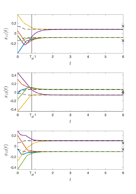
Figure 2: Entry-wise trajectory of each agent for the multi-agent system (6) under the structurally balanced matrix-weighted network $\mathcal{G}_{1}$ in Figure 1.

6 Simulations

In this section, we proceed to provide simulation examples to demonstrate the effectiveness of the proposed event-triggered coordination strategy.

6-A Leaderless Matrix-weighted Networks

First, consider the leaderless multi-agent system (6) on the structurally balanced matrix-weighted network $\mathcal{G}_{1}$ in Figure 1. The solid lines represent the edges weighted by (positive or negative) definite matrices, the dashed lines represent the edges weighted by (positive or negative) semi-definite matrices. The blue lines represent edges weighted by positive (semi-)definite matrices, and red lines represent edges weighted by negative (semi-)definite matrices. The node bipartition of $\mathcal{G}_{1}$ is $\mathcal{V}_{1}=\{1,2,5\}$ and $\mathcal{V}_{2}=\{3,4\}$.

In this example, the state dimension of each agent is $d=3$, and all agents adopt event-triggered control protocol (4). The edges in $\mathcal{G}_{1}$ are weighted by

$$A_{12}=\begin{bmatrix}10.14&1.64&-2.16\\ 1.641&\text{10.06}&-1.58\\ -2.16&-1.58&12.45\end{bmatrix}>0,$$

$$A_{23}=\begin{bmatrix}-9.75&1.87&4.69\\ 1.87&-7.17&0.72\\ 4.69&0.72&-9.51\end{bmatrix}<0,$$

$$A_{15}=\begin{bmatrix}12.42&-1.51&-1.07\\ -1.51&11.52&-1.1\\ -1.07&-1.1&14.4\end{bmatrix}>0,$$

$$A_{25}=\begin{bmatrix}3.03&-2.21&3.92\\ -2.21&4.58&-1.63\\ 3.92&-1.63&5.6\end{bmatrix}\geq 0,$$

$$A_{34}=\begin{bmatrix}7.36&4.67&5.13\\ 4.67&10.89&-2.31\\ 5.13&-2.31&9.92\end{bmatrix}>0,$$

and

$$A_{45}=\begin{bmatrix}-4.88&-3.07&0.46\\ -3.07&-2.82&-2.03\\ 0.46&-2.03&-6.13\end{bmatrix}\leq 0.$$

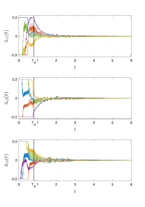
Figure 3: The event-based control protocol $\widehat{\boldsymbol{u}}_{i}(t)$ of each agent $i\in\mathcal{V}$ for the multi-agent system (6) under the structurally balanced matrix-weighted network $\mathcal{G}_{1}$.

Moreover, $A_{ij}=A_{ji}$ for all $(i,j)\in\mathcal{E}(\mathcal{G}_{1})$. Let the saturation level be $\triangle=0.5$. Choose $\rho_{i}=0.9$, $\delta_{i}=1$, $\beta_{i}=1$, and $\psi_{i}(0)=0.5$. By computing the eigenvalues of the weight matrices, one has $\varpi_{1}=6620$, $\varpi_{2}=10212$, $\varpi_{3}=6355$, $\varpi_{4}=3880$ and $\varpi_{5}=7144$. According to Theorem 8, one can choose $\theta_{i}=0.5$ which satisfies $\theta_{i}>\frac{1-\delta_{i}}{\beta_{i}}$. Each dimension of initial value corresponding to each agent is randomly chosen from the interval $[-1,1]$. Using the above parameters, the global bipartite consensus can be achieved in an element-wise manner, as shown in Figure 2. The dimensions of control protocol for each agent are illustrated in Figure 3. Sequences of triggering time for each agent are illustrated in Figure 4.

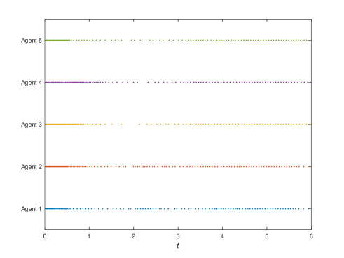
Figure 4: The triggering time instants of each agent in the multi-agent system (6) under the structurally balanced matrix-weighted network $\mathcal{G}_{1}$.

Note that the multi-agent system does not achieve average bipartite consensus, indicated by black crosses at $t=6$ in Figure 2. The simultaneous average (after a proper gauge transformation) of agents’ states is shown in separate dimension in Figure 2, highlighted by black dashed lines in each panel. Note that this average value may vary when the each agent is driven by saturated input. As one can observe that, the multi-agent system behaves in a manner of saturation-free after $t=T_{\text{sf}}=0.8$. In this example, the final bipartite consensus value is the average (after a proper gauge transformation) of $\boldsymbol{x}(0.8)$, namely, $D^{*}(\boldsymbol{1}_{n}\otimes(\frac{1}{n}(\boldsymbol{1}_{n}^{T}\otimes I_{d})D^{*}\boldsymbol{x}(0.8)))$. The black solid vertical line in each panel of Figure 2 and Figure 3 indicates the $T_{\text{sf}}$, namely, the last time instance that there exists saturated control inputs in the multi-agent system.

6-B Leader-follower Matrix-weighted Networks

Consider the leader-follower multi-agent system (19) on the leader-follower network $\mathcal{G}_{1}^{\prime}$ in Figure 5, where agents $1$ and $5$ are the leaders influenced by the inputs $\boldsymbol{w}_{1}$ and $\boldsymbol{w}_{2}$, respectively. The edge weights on the matrix-weighted network $\mathcal{G}_{1}^{\prime}$ are the same as the leaderless case above, the influence weights by the inputs $\boldsymbol{w}_{1}$ and $\boldsymbol{w}_{2}$ are $B_{11}=A_{25}\geq 0,$ and $B_{52}=A_{12}>0,$ respectively.

Figure 5: A structurally balanced matrix-weighted network with two external inputs $w_{1}$ and $w_{2}$, denoted by $\mathcal{G}_{1}^{\prime}$. The correspondence between the line pattern and weight matrix is the same as that in Figure 1.

In this case, choose $\rho_{i}=0.9$, $\delta_{i}=1$, $\beta_{i}=1$, $\psi_{i}(0)=0.5$, and $\boldsymbol{w}_{1}=\boldsymbol{w}_{2}=[0.2,0.4,0.6]^{T}$. Let the saturation constraint be $\triangle=0.5$. By computing the eigenvalues of the weight matrices, one has $\omega_{1}=10004$, $\omega_{2}=10212$, $\omega_{3}=6355$, $\omega_{4}=3880$, $\omega_{5}=13027$.

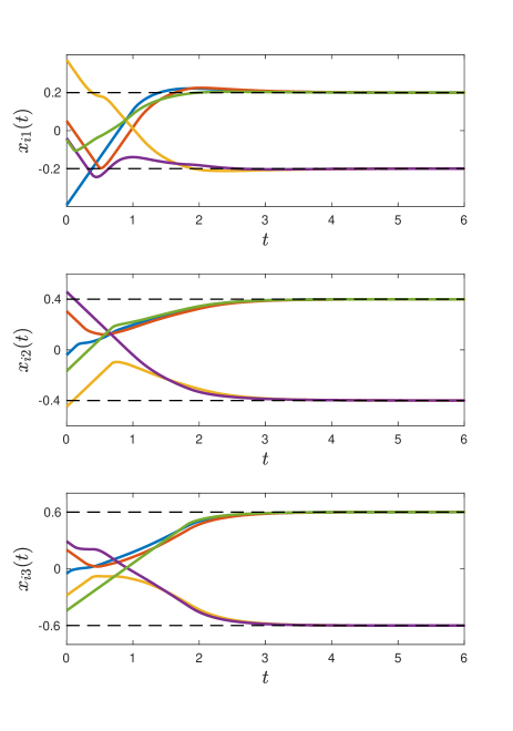
Figure 6: Entry-wise trajectory of each agent for the multi-agent system (19) under the leader-follower network $\mathcal{G}_{1}^{\prime}$ in Figure 5.

According to Theorem 15, choose $\theta_{i}=1$ satisfying $\theta_{i}>\frac{1-\delta_{i}}{\beta_{i}}$.

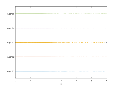
Figure 7: The triggering time instants of each agent in the multi-agent system (19) under the leader-follower network $\mathcal{G}_{1}^{\prime}$ in Figure 5.

Under these parameters, the global bipartite leader-follower consensus can be achieved as shown in Figure 6. Sequences of triggering time for each agent are demonstrated in Figure 7. The dimensions of control protocol for each agent are illustrated in Figure 8.

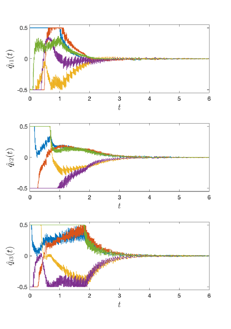
Figure 8: The event-based control protocol $\widehat{\boldsymbol{q}}_{i}(t)$ of each agent $i\in\mathcal{V}$ for the multi-agent system (19) under the leader-follower network $\mathcal{G}_{1}^{\prime}$ in Figure 5.

7 Conclusion

In this paper, we examined the event-triggered global bipartite consensus problem for multi-agent systems on matrix-weighted networks subject to input saturation constraints. Dynamic event-triggered distributed protocols for both leaderless and leader-follower cases are provided, where each agent only needs to broadcast at its own state on triggering times, and listen to incoming information from its neighbors at their triggering times, which reduces the limited communication resource and avoids the continuous communication among agents. Then, some criteria are derived to guarantee the leaderless and leader-follower global bipartite consensus of the multi-agent systems. Also, the proposed triggering laws are shown to be free of Zeno phenomenon by proving that the triggering time sequence of each agent is divergent. Simulation examples demonstrate the effectiveness of the proposed methods.

References

- [1] Z. Sun and C. B. Yu, “Dimensional-invariance principles in coupled dynamical systems: A unified analysis and applications,” IEEE Transactions on Automatic Control, vol. 64, no. 8, pp. 3514–3520, 2018.
- [2] L. Pan, H. Shao, Y. Xi, and D. Li, “Bipartite consensus problem on matrix-valued weighted directed networks,” Science China Information Sciences, vol. 64, no. 4, pp. 1–3, 2021.
- [3] L. Pan, H. Shao, M. Mesbahi, Y. Xi, and D. Li, “Bipartite consensus on matrix-valued weighted networks,” IEEE Transactions on Circuits and Systems II: Express Briefs, vol. 66, no. 8, pp. 1441–1445, 2019.
- [4] M. H. Trinh, C. Van Nguyen, Y.-H. Lim, and H.-S. Ahn, “Matrix-weighted consensus and its applications,” Automatica, vol. 89, pp. 415–419, 2018.
- [5] M. Mesbahi and M. Egerstedt, Graph Theoretic Methods in Multiagent Networks. Princeton University Press, 2010.
- [6] R. Olfati-Saber, A. Fax, and R. M. Murray, “Consensus and cooperation in networked multi-agent systems,” Proceedings of the IEEE, vol. 95, no. 1, pp. 215–233, 2007.
- [7] P. Barooah and J. P. Hespanha, “Graph effective resistance and distributed control: Spectral properties and applications,” in 45th IEEE conference on Decision and control, pp. 3479–3485, 2006.
- [8] S. E. Tuna, “Observability through a matrix-weighted graph,” IEEE Transactions on Automatic Control, vol. 63, no. 7, pp. 2061–2074, 2017.
- [9] N. E. Friedkin, A. V. Proskurnikov, R. Tempo, and S. E. Parsegov, “Network science on belief system dynamics under logic constraints,” Science, vol. 354, no. 6310, pp. 321–326, 2016.
- [10] S. Zhao and D. Zelazo, “Translational and scaling formation maneuver control via a bearing-based approach,” IEEE Transactions on Control of Network Systems, vol. 4, no. 3, pp. 429–438, 2015.
- [11] S. E. Tuna, “Synchronization under matrix-weighted Laplacian,” Automatica, vol. 73, pp. 76–81, 2016.
- [12] H. Su, J. Chen, Y. Yang, and Z. Rong, “The bipartite consensus for multi-agent systems with matrix-weight-based signed network,” IEEE Transactions on Circuits and Systems II: Express Briefs, 2019.
- [13] S. Miao and H. Su, “Second-order consensus of multiagent systems with matrix-weighted network,” Neurocomputing, vol. 433, pp. 1–9, 2021.
- [14] C. Wang, L. Pan, D. Li, H. Shao, and Y. Xi, “Consensus of second-order matrix-weighted multi-agent networks,” in 2020 16th International Conference on Control, Automation, Robotics and Vision (ICARCV), pp. 590–595, IEEE, 2020.
- [15] Y. Li and Z. Lin, Stability and performance of control systems with actuator saturation. Springer, 2018.
- [16] T. Hu and Z. Lin, Control systems with actuator saturation: analysis and design. Springer Science & Business Media, 2001.
- [17] H. Sussmann, E. Sontag, and Y. Yang, “A general result on the stabilization of linear systems using bounded controls,” in Proceedings of 32nd IEEE Conference on Decision and Control, pp. 1802–1807, IEEE, 1993.
- [18] X. Wang and M. D. Lemmon, “Event-triggering in distributed networked control systems,” IEEE Transactions on Automatic Control, vol. 56, no. 3, pp. 586–601, 2010.
- [19] K. J. Åström and B. Bernhardsson, “Comparison of periodic and event based sampling for first-order stochastic systems,” IFAC Proceedings Volumes, vol. 32, no. 2, pp. 5006–5011, 1999.
- [20] Y. Li, J. Xiang, and W. Wei, “Consensus problems for linear time-invariant multi-agent systems with saturation constraints,” IET Control Theory & Applications, vol. 5, no. 6, pp. 823–829, 2011.
- [21] Z. Meng, Z. Zhao, and Z. Lin, “On global leader-following consensus of identical linear dynamic systems subject to actuator saturation,” Systems & Control Letters, vol. 62, no. 2, pp. 132–142, 2013.
- [22] T. Yang, Z. Meng, D. V. Dimarogonas, and K. H. Johansson, “Global consensus for discrete-time multi-agent systems with input saturation constraints,” Automatica, vol. 50, no. 2, pp. 499–506, 2014.
- [23] H. Su, M. Z. Chen, J. Lam, and Z. Lin, “Semi-global leader-following consensus of linear multi-agent systems with input saturation via low gain feedback,” IEEE Transactions on Circuits and Systems I: Regular Papers, vol. 60, no. 7, pp. 1881–1889, 2013.
- [24] Z. Lin, Low gain feedback. Springer, 1999.
- [25] L. Ding, Q.-L. Han, X. Ge, and X.-M. Zhang, “An overview of recent advances in event-triggered consensus of multiagent systems,” IEEE transactions on cybernetics, vol. 48, no. 4, pp. 1110–1123, 2017.
- [26] C. Nowzari, E. Garcia, and J. Cortés, “Event-triggered communication and control of networked systems for multi-agent consensus,” Automatica, vol. 105, pp. 1–27, 2019.
- [27] D. V. Dimarogonas, E. Frazzoli, and K. H. Johansson, “Distributed event-triggered control for multi-agent systems,” IEEE Transactions on Automatic Control, vol. 57, no. 5, pp. 1291–1297, 2011.
- [28] C. Nowzari and J. Cortés, “Distributed event-triggered coordination for average consensus on weight-balanced digraphs,” Automatica, vol. 68, pp. 237–244, 2016.
- [29] X. Yi, K. Liu, D. V. Dimarogonas, and K. H. Johansson, “Dynamic event-triggered and self-triggered control for multi-agent systems,” IEEE Transactions on Automatic Control, vol. 64, no. 8, pp. 3300–3307, 2018.
- [30] G. A. Kiener, D. Lehmann, and K. H. Johansson, “Actuator saturation and anti-windup compensation in event-triggered control,” Discrete event dynamic systems, vol. 24, no. 2, pp. 173–197, 2014.
- [31] X. Wu and T. Yang, “Distributed constrained event-triggered consensus: L 2 gain design result,” in IECON 2016-42nd Annual Conference of the IEEE Industrial Electronics Society, pp. 5420–5425, IEEE, 2016.
- [32] X. Yin, D. Yue, and S. Hu, “Adaptive periodic event-triggered consensus for multi-agent systems subject to input saturation,” International Journal of Control, vol. 89, no. 4, pp. 653–667, 2016.
- [33] X. Yi, T. Yang, J. Wu, and K. H. Johansson, “Distributed event-triggered control for global consensus of multi-agent systems with input saturation,” Automatica, vol. 100, pp. 1–9, 2019.
- [34] F. Harary et al., “On the notion of balance of a signed graph.,” The Michigan Mathematical Journal, vol. 2, no. 2, pp. 143–146, 1953.
- [35] C. Altafini, “Consensus problems on networks with antagonistic interactions,” IEEE Transactions on Automatic Control, vol. 58, no. 4, pp. 935–946, 2013.
- [36] H. K. Khalil, Nonlinear Systems. Prentice Hall, 2002.
- [37] M. H. Trinh, M. Ye, H.-S. Ahn, and B. D. Anderson, “Matrix-weighted consensus with leader-following topologies,” in 2017 11th Asian Control Conference (ASCC), pp. 1795–1800, IEEE, 2017.