Cell Zooming with Masked Data for Off-Grid Small Cell Networks: Distributed Optimization Approach

Abstract

Cell zooming has been becoming an essential enabler for off-grid small cell networks. Traditional models often utilize the numbers of active users in order to determine cell zooming strategies. However, such confidential measurement data must be concealed from others. We therefore propose a novel cell zooming method with masking noise. The proposed algorithm is designed based on distributed optimization, in which each SBS locally solves a divided optimization problem and learns how much a global constraint is satisfied or violated for temporal solutions. The important feature of this distributed control method is robustness against masking noise. We analyze the trade-off between confidentiality and optimization accuracy, using the notion of differential privacy. Numerical simulations show that the proposed distributed control method outperforms a standard centralized control method in the presence of masking noise.

I Introduction

Off-grid small cell base stations (SBSs) are expected to be a promising technology that can boost the capability of traditional macro cell base stations (MBSs) with minimum capital expenditures and operating expenses [1, 2]. Off-grid SBSs achieve sustainable operation without power grids by employing energy harvesting modules such as solar photovoltaics. LG U+ and China Mobile deployed off-grid base stations (BSs) and started the communications services [3]. The study [4] reports that a solar panel with an area of $0.6\,\text{m}^{2}$ can harvest up to $500\,\mathrm{W}$ with a conversion efficiency of $14\,\%$. Although the level of energy harvesting is high enough to operate SBSs, energy harvesting conditions strongly depend on time and location. Therefore, it is important to control the operation of off-grid SBSs according to energy harvesting conditions.

As a fundamental problem of off-grid SBSs, cell zooming from the operator’s point of view has been under intensive investigation for the past several years. Previous studies on cell zooming can be classified into a physical-layer solution [5, 6, 7, 8, 9, 3] and a network-layer solution [10, 11, 12, 13, 14, 15, 16, 17, 18, 19, 20] based on their objectives.

The physical-layer solution aims at maximizing physical-layer wireless capability such as capacity and energy efficiency by using channel state information and battery state information. In this approach, the network operation is optimized without taking user demands into account. An et al. [5] study the impact of SBS density on the energy efficiency in cellular networks by the stochastic geometry theory and propose an optimal user association strategy based on quantum particle swarm optimization. The capacity of energy harvesting small cells is maximized via joint sleep-wake scheduling and transmission power control in [6]. Maghsudi and Hossain [7] investigate a distributed user association problem of downlink small cell networks, where SBSs select users by maximizing their successful transmission probability. In [8], a small cell network is modeled as a competitive market with uncertainty so as to develop a distributed user association scheme for energy harvesting small cell networks under uncertainty. Liu et al. [9] develop a mathematical model to assess the association probabilities and coverage probabilities of non-uniform off-grid small cell networks with cell zooming. Ko et al. [3] propose a novel architecture of off-grid small cell networks where SBSs employ wireless power transfer to share their harvested energy with the terminals of accommodated users.

The objectives of the network-layer solution are to guarantee the quality of services such as delay and throughput and to minimize an operation cost. In addition to channel state information and battery state information, this approach exploits traffic load, user distribution, service types, and so on. In other words, the network-layer solution is based on the dynamics of user’s behaviors as well as channel state information and battery state information. Zhang et al. [10] propose an energy-efficient cell zooming method, in which user association, SBSs activation, and power control are jointly optimized based on battery state information and user demands. The performance of network-layer cell zooming depends on the accuracy of traffic load estimation. To overcome this difficulty, an estimation scheme based on various kinds of big data is proposed in [11]. Model predictive control is applied to an online cell zooming problem in [12], which allows small cell networks to provide sustainable communication to users with optimal energy efficiency. Chamola et al. [13] demonstrate that energy efficiency and communication latency can be improved by a cell zooming technique in a real BS deployment scenario. A recent trend in network-layer solutions is to design a fast algorithm to solve a non-convex optimization problem of cell zooming by using the ski rental problem [14], network centrality [15], and layered learning [16]. Another recent trend is to develop a novel paradigm of off-grid small cell networks, e.g., wireless mesh networks consisting of off-gird SBSs [17], content-aware cell zooming [18], vehicular edge computing [19], and energy sharing among SBSs [20].

One of the main drawbacks of the existing studies above is that they do not consider the security of control systems. To determine a cell zooming policy, a central controller, which is mostly contained in an MBS, collects the numbers of active users in the service areas of SBSs. Such social data can be also used for commercial and administrative purposes, e.g., to find socioeconomic trends, to design public transportation systems, and to analyze people-flow after catastrophic events such as earthquakes for the mitigation of secondary disasters [21, 22]. To steal the confidential measurement data, intruders may do packet sniffing (see, e.g., [23, 24]), i.e., analyze control packets transmitted from SBSs. To prevent security threats and commercial losses, mobile network providers need to carefully protect the confidentiality of the measurement data. Adding masking noise to the measurement data is a simple method to enhance the security of cell networks but simultaneously worsens the performance of cell zooming. To the best of our knowledge, there is no literature on noise-resistant cell zooming techniques.

This research is classified into a network-layer solution. We formulate the minimization problem of cell zooming for off-grid SBSs and assume that intruders can analyze control packets but have no knowledge of controllers or data correlation. In the minimization problem, two elements are evaluated: the user association by the SBSs and the available energy of batteries in the SBSs. Since the SBSs are powered by energy harvesting devices, the cell network becomes more “green” as the number of users associated with the SBSs increases. On the other hand, the depletion of the energy in the SBSs should be avoided for the sustainable operation of the cell network. For these reasons, we consider the above two elements in the minimization problem of cell zooming.

Distributed optimization plays a key role in the proposed cell zooming method. Each SBS locally solves a divided optimization problem, and the central controller only checks whether or not the temporal control policies computed by the SBSs achieve the global constraint, i.e., the full accommodation of active users. The SBSs know only local information but learn the extent to which the global constraint is satisfied or violated for the temporal control policies. The essential idea of distributed optimization we use can be found in [25, Chapter 5]. We refer the reader to [26, 27] for the recent developments of distributed optimization.

Reduction of computational complexity is an important issue in the distributed method, because each SBS, which generally has limited computational resources, solves a divided optimization problem iteratively. However, the minimization problem originally formulated for cell zooming is equivalent to a mixed integer nonlinear programing problem due to the discrete behavior of sleep-wake scheduling. To reduce computational complexity, we apply the $\ell^{1}$ convex relaxation [28] and analyze the divided optimization problem each SBS solves.

The main contributions of this paper are as follows:

• We develop a distributed cell zooming method that is robust to masking noise. In the conventional centralized control method, both the objective function and the constraint of the minimization problem are negatively affected by masking noise. In contrast, only the constraint is disturbed by masking noise in the distributed control method. Therefore, the proposed method is less susceptible to masking noise than the conventional centralized method, which is also verified from numerical simulations.

• As a by-product of the distributed control approach, we can simultaneously determine the transmission powers and the sleep-wake schedules of the SBSs. Moreover, the distributed approach can deal with the situation where the user densities in the areas of the SBSs are different. The centralized cell zooming method based on model predictive control [12] does not have these features.

• We propose a computationally-efficient algorithm to solve the minimization problem of cell zooming. The proposed algorithm finds an approximate solution with low computational complexity. Numerical results show that the approximation error is quite small.

• We analyze the trade-off between confidentiality and optimization accuracy, by using the notion of differential privacy [29] as a measure of confidentiality. This trade-off analysis can be used as a guideline to determine the noise intensity for cell zooming with masked data.

The rest of this paper is organized as follows. In Section II, we formulate the minimization problem of cell zooming and then compare the effects of masking noise between the centralized and distributed control methods. In Section III, we develop a distributed algorithm for cell zooming with masked data. Section IV is devoted to analyzing the trade-off between confidentiality and optimization accuracy. In Section V, we evaluate the performance of the distributed control method, using numerical examples. Section VI concludes the paper.

The proposed method is based on the technique developed in our conference paper [30]. The new parts in the journal version are as follows. First, we provide numerical simulations to show how resistant the distributed control method is to masking noise. Second, we significantly reduce the computational complexity of the distributed control method by developing an explicit formula for an approximate solution of the divided optimization problem. Finally, the analysis of the trade-off between confidentiality and optimization accuracy is completely new.

II System Model and Problem Formulation

In this section, we first describe the power flow and the user association of off-grid SBSs. Next we formulate the minimization problem of cell zooming for SBSs. Finally, we compare centralized and distributed control approaches from the viewpoint of robustness against masking noise. The main notations used in this article are summarized in Table I.

II-A Power flow of SBS

Let us consider that $N$ SBSs are deployed within the coverage region of an MBS powered by the grid. The SBSs are off-grid and equipped with an energy harvesting device and a battery for energy storage. We denote by $w_{i}[k]$ the harvested power [W] of the $i$th SBS at time $k$. The SBSs consume the energy of the battery for the transmission power and the system power. Let $u_{i}[k]$ and $s_{i}[k]$ denote the transmission power [W] and the system power [W] of the $i$th SBS at time $k$, respectively. Then the power consumption of the $i$th SBS at time $k$ is given by $u_{i}[k]/\gamma+s_{i}[k]$, where a positive quantity $\gamma$ is a power amplifier efficiency. The system power $s_{i}[k]$ takes two values, depending on whether the SBS is in an active mode or a sleep mode:

$$s_{i}[k]:=\begin{cases}s_{\text{active}}&\text{if $u_{i}[k]>0$ ~{}($i$th SBS is active)},\\ s_{\text{sleep}}&\text{if $u_{i}[k]=0$ ~{}($i$th SBS is sleep)}.\end{cases}$$ (1)

Notice that the SBS is in the sleep mode if and only if the transmission power is set to $0$.

The power flow of the battery in the $i$th SBS at time $k$ (positive in charging) is described by $w_{i}[k]-u_{i}[k]/\gamma-s_{i}[k].$ Let $x_{i}[k]\in[0,X_{\max}]$ be the residual energy [J] of the $i$th SBS at time $k$. The energy $x_{i}[k]$ has the dynamics:

$$x_{i}[k+1]=\mathop{\rm sat}\Big{(}x_{i}[k]+h\big{(}w_{i}[k]-u_{i}[k]/\gamma-s_{i}[k]\big{)}\Big{)},$$ (2)

where a positive quantity $h$ is a sampling period [s] and a function $\mathop{\rm sat}:\mathbb{R}\to[0,X_{\max}]$ is the saturation function defined by

$$\mathop{\rm sat}(x):=\begin{cases}0&\text{if $x<0$},\\ x&\text{if $x\in[0,X_{\max}]$},\\ X_{\max}&\text{if $x>X_{\max}$}.\\ \end{cases}$$ (3)

Fig. 1 shows the power flow of the SBSs.

TABLE I: List of main notations.

Notation	Definition
$N$	Number of SBSs
$x_{i}$	Residual energy of $i$th SBS
$u_{i}$	Transmission power of $i$th SBS
$w_{i}$	Harvested power of $i$th SBS
$s_{i}$	System power of $i$th SBS
$v_{i}$	Masking noise for $i$th SBS
$s_{\rm active}$	System power in active mode
$s_{\rm sleep}$	System power in sleep mode
$X_{\max}$	Maximum capacity of battery
$\gamma$	Amplifier efficiency
$h$	Sampling period
$\mathop{\rm sat}$	Saturation function: $\mathbb{R}\to[0,X_{\max}]$
$U_{\rm Macro}$	Maximum capacity of MBS
$U_{i}$	Number of users in $i$th SBS area
$A$	Size of SBS coverage area
$F$	Number of users served by one SBS
$\bf u$	Vector of transmission powers
$\bf U$	Vector of numbers of users
$\bf v$	Vector of masking noise
$P_{k}$	Objective function at time $k$
$\lambda$	Weighting parameter of $P_{k}$
P	Probability
E	Expectation
$\mathop{\rm Lap}(\rho)$	Laplace distribution with parameter $\rho$
$\|u\|_{i}$	$\ell^{i}$ norm of $u$ ($i=0,1,2$)

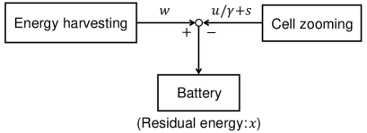
Figure 1: Power flow of SBS.

II-B User association

Let $U_{\text{Macro}}$ be the maximum number of users associated with the MBS and $U_{i}[k]$ be the number of users who request communication services in the coverage area of the $i$th SBS at time $k$. Let $A$ be the size [$\text{km}^{2}$] of the coverage area of each SBS. We assume that active users are uniformly distributed in the coverage areas. Let $F(u,U)$ denote the number of users who an SBS can accommodate by the transmission power $u$ in its service area with $U$ users. In [31], a formula for $F(u,U)$ is given by

$$F(u,U):=rUu^{\frac{10}{19}},$$ (4)

where a positive quantity $r$ is given by $r:=\pi 10^{b+\frac{30}{19}}/A$ with

$$b:=-\frac{1}{19}\left(\frac{5}{2}\mathrm{erfc}^{-1}\left(\frac{8}{3}\mathrm{BER}(Q)\right)^{2}+\sigma+Z\right).$$ (5)

In this definition, $\sigma$, $Z$, and $\mathrm{BER}(Q)$ are the system noise [dBm] at a user device, the path loss factor [dBm] other than distance related factor in the Walfisch-Ikegami model, and the bit error rate satisfying the desired QoE value $Q$, respectively. The function $\mathrm{BER}(Q)$ is defined by

$$\mathrm{BER}(Q):=1-{\rm exp}\left(\frac{1}{S}\ln\left(1+\frac{1}{4.473}\ln\left(\frac{Q-1.065}{3.01}\right)\right)\right),$$ (6)

where $S$ denotes the packet size [bit] in data transmission.

We consider the scenario where the SBSs first accommodate the users in their service areas and then the MBS serves the rest of the users. Because SBSs are deployed such that they cover disjoint areas due to cost efficiency, the sum of the numbers of users is given by $\sum_{i=1}^{N}U_{i}$, and the sum of the numbers of users associated with the SBSs is $\sum_{i=1}^{N}F(u_{i},U_{i})$.

II-C Optimization problem for cell zooming

The objective of cell zooming is to determine the transmission powers and the sleep-wake schedules of the SBSs. The following two elements are evaluated in the objective function of cell zooming.

1. The SBSs use renewable energy in their operation, whereas the MBS consumes energy from the grid. To make the cell network “green,” we should leverage the SBSs. Therefore, we minimize the number of users not associated with the SBS, $U_{i}[k]-F(u_{i}[k],U_{i}[k]).$

2. The energy depletion of the SBSs may severely degrade the service quality. It is preferable that the residual energy of each SBS is close to the full charge state $X_{\rm max}$. In other words, we have to keep the difference $X_{\max}-x_{i}[k+1]$ small, when determining a cell zooming policy at time $k$.

The objective function $P_{k}$ at time $k$ is given by a weighted squared sum of the above two terms:

$$P_{k}\big{(}{\bf u},{\bf U}[k]\big{)}:=\sum_{i=1}^{N}\bigg{[}\Big{(}U_{i}[k]-F\big{(}u_{i},U_{i}[k]\big{)}\Big{)}^{2}$$

$$+\lambda\Big{(}X_{\max}-\mathop{\rm sat}\big{(}x_{i}[k]+h(w_{i}[k]-u_{i}/\gamma-s_{i})\big{)}\Big{)}^{2}~{}\!\bigg{]},$$ (7)

where

$${\bf u}:=\begin{bmatrix}u_{1}&\cdots&u_{N}\end{bmatrix},\quad{\bf U}[k]:=\begin{bmatrix}U_{1}[k]&\cdots&U_{N}[k]\end{bmatrix}.$$ (8)

Here a positive quantity $\lambda$ is a weighting parameter. If this parameter is small, then the control policy places more importance on the number of users associated with the SBSs but less importance on the residual energy.

The optimization problem of cell zooming can be formulated mathematically as follows:

$$\min_{\bf u}~{}P_{k}\big{(}{\bf u},{\bf U}[k]\big{)}$$ (9)

s.t. $$~{}\text{[C1]~{}~{}}u_{i}\geq 0,\quad 1\leq i\leq N,$$

$$~{}\text{[C2]~{}~{}}s_{i}=\begin{cases}s_{\text{active}}&\text{if $u_{i}>0$},\\ s_{\text{sleep}}&\text{if $u_{i}=0$},\end{cases}\quad 1\leq i\leq N,$$

$$~{}\text{[C3]~{}~{}}x_{i}[k]+h(w_{i}[k]-u_{i}/\gamma-s_{i})\geq 0,\quad 1\leq i\leq N,$$

$$~{}\text{[C4]~{}~{}}U_{i}[k]-F\big{(}u_{i},U_{i}[k]\big{)}\geq 0,\quad 1\leq i\leq N,$$

$$~{}\text{[C5]~{}~{}}\sum_{i=1}^{N}\Big{(}U_{i}[k]-F\big{(}u_{i},U_{i}[k]\big{)}\Big{)}\leq U_{\rm Macro}.$$

In the above minimization problem, [C1] is the non-negativity constraint on transmission powers, and [C2] means that the system power takes only two discrete values depending on whether the SBS is in the active mode or the sleep mode. By [C3], a cell zooming policy is determined to avoid the energy shortage of the SBSs. If there exists no transmission power $u_{i}\geq 0$ satisfying this constraint, we deactivate the $i$th SBS, i.e., set $u_{i}=0$ and $s_{i}=s_{\text{sleep}}$. The constraint [C4] means that the $i$th SBS determines its transmission power so that it accommodates at most $U_{i}[k]$ users. If this constraint is violated, then the SBSs waste their energy because the transmission powers are unnecessarily large. By [C5], the MBS can accommodate all the users who are not associated with the SBSs.

It is challenging to solve the minimization problem (9) in real time due to the constraint [C2]. Indeed, using an auxiliary integer variable $q_{i}\in\{0,1\}$, we can rewrite the constraint [C2] as

$$q_{i}u_{i}=0,~{}~{}-q_{i}<u_{i},~{}~{}s_{i}=(1-q_{i})s_{\text{active}}+q_{i}s_{\text{sleep}}.$$ (10)

Therefore, the minimization problem (9) is equivalent to a mixed-integer nonlinear programming problem.

II-D Importance of data masking

We consider the situation where intruders can analyze control packets sent by the SBSs and the MBS but not have any prior knowledge of controllers or correlation between data. To solve the minimization problem (9), the numbers of users, $U_{1}[k],\dots,U_{N}[k]$, are transmitted from the SBSs to the MBS. The leakage of such social data leads to security threats and commercial losses. To avoid it, the $i$th SBS sends not the raw data $U_{i}[k]$ but the masked data $U_{i}[k]+v_{i}[k]$, where $v_{i}[k]$ is the masking noise for the $i$th SBS at time $k$. As the masking noise becomes larger, it is more difficult for intruders to find the exact value of the confidential measurement data. However, large masking noise degrades the performance of cell zooming. The objective of this paper is to develop a cell zooming method that is robust against masking noise.

II-E Comparison between centralized and distributed methods with masking noise

In the case of centralized control, the central controller (often in the MBS) needs to collect the information on the residual energy $x_{i}$, the harvested energy $w_{i}$, and the number of users $U_{i}$ from the $i$th SBS for solving the minimization problem (9). Since $U_{i}$ is confidential data, each SBS adds the noise $v_{i}$ to $U_{i}$ and send the masked data $U_{i}+v_{i}$ to the central controller. Fig. 2(a) illustrates the information flow of the centralized case. The resulting minimization problem that the central controller solves is given by

$$\min_{\bf u}~{}P_{k}\big{(}{\bf u},{\bf U}[k]+{\bf v}[k]\big{)}$$ (11)

s.t. $$\text{[C1]\hskip 1.0pt--\hskip 1.0pt[C4]},$$

[C5 with noise]

$$\sum_{i=1}^{N}\Big{(}U_{i}[k]+v_{i}[k]-F\big{(}u_{i},U_{i}[k]+v_{i}[k]\big{)}\Big{)}\leq U_{\rm Macro},$$

where

$${\bf v}[k]:=\begin{bmatrix}v_{1}[k]&\cdots&v_{N}[k]\end{bmatrix}.$$

Notice that [C4] is not affected by the masking noise because

$$U+v-F(u,U+v)\geq 0$$

if and only if $u\leq r^{-\frac{19}{10}}$ for every $v>-U$. In the above minimization problem, both the objective function and the constraint [C5] contain the noise. Therefore, the solution of the minimization problem (11) may have a large error due to the masking noise.

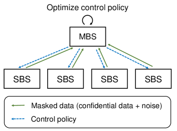
(a) Centralized case.

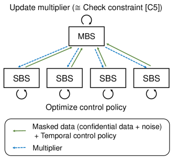
(b) Distributed case.

Figure 2: Information flow.

The proposed method employs distributed optimization. In the distributed approach, the objective function $P_{k}$ is divided into $N$ local functions and is minimized locally in each SBS. Consequently, the masking noise affects only the constraint [C5], which makes the proposed method resistant to masking noise.

As shown in Fig. 2(b), each SBS locally solves a divided minimization problem, and the central controller simply checks whether the global constraint [C5] is satisfied for the masked data $U_{i}+v_{i}$ and the temporal control policy transmitted from each SBS. Updating a multiplier in Fig. 2(b) represents this action of the central controller, because we apply the duality principle (see, e.g., [25, Chapter 5]) to the minimization problem. From the updated multiplier, the SBSs, which know only local data, learn the extent to which the global constraint [C5] is satisfied or violated, and then update the control policy based on this learning. A detailed discussion on it is provided in Section III-B.

Remark II.1

Wada and Sakurama [32] propose a masking method to protect the agent privacy for distributed optimization, where an “agent” is an SBS in our cell zooming problem. By this method, each agent conceals private information from other agents without any influence on solutions of optimization problems. Its essential idea is to exchange masking signals between neighbor agents. However, it does not work in our setting where intruders analyze control packets transmitted from the SBSs.

III Distributed Cell Zooming

In this section, we propose a distributed cell zooming algorithm. First, we approximate the minimization problem (9) formulated in the previous section. Using the approximate problem, we next apply a distributed optimization technique to cell zooming for off-grid SBSs. Finally, we analyze the divided minimization problem that each SBS iteratively solves in the distributed algorithm.

III-A Approximation techniques

It is important in distributed cell zooming to reduce computational complexity. The reason is that a divided minimization problem is iteratively solved by each SBS, which has limited computational resources in general. Computing the exact solution of the originally formulated minimization problem (9) requires significant computational resources. Hence we first develop approximation techniques to reduce the computational complexity.

III-A1 Omission of saturation function

The saturation function $\mathop{\rm sat}$ in the second term of the objective function $P_{k}$ has little effect on solutions, and therefore we omit it. In fact, by the constraint [C3], the input of $\mathop{\rm sat}$,

$$x_{i}[k]+h(w_{i}[k]-u_{i}/\gamma-s_{i}),$$ (12)

is non-negative, and hence we can omit the lower bound of $\mathop{\rm sat}$. Moreover, the omission of the upper bound of $\mathop{\rm sat}$ yields only a small approximation error. This is because if the residual energy is close to $X_{\max}$, then the corresponding transmission power is set to a large value so that the input of $\mathop{\rm sat}$ given in (12) becomes smaller than the upper bound $X_{\max}$. The omission of $\mathop{\rm sat}$ makes the minimization problem easy to deal with, because this function is not convex or concave; see the definition (3).

III-A2 Convex relaxation by $\ell^{1}$ norm

By the omission of the saturation function, the second term of $P_{k}$ can be rewritten as

$$\big{(}X_{\max}-x_{i}[k]-h(w_{i}[k]-u_{i}/\gamma-s_{i})\big{)}^{2}$$

$$\quad=(X_{\max}-x_{i}[k]-hw_{i}[k]+hu_{i}/\gamma)^{2}+h^{2}s_{i}^{2}$$ (13)

$$\qquad+2h(X_{\max}-x_{i}[k]-hw_{i}[k]+hu_{i}/\gamma)s_{i}.$$

Using the $\ell^{0}$ norm $\|{\bf u}\|_{0}$, we obtain

$$\sum_{i=1}^{N}h^{2}s_{i}^{2}=h^{2}\big{(}s_{\rm active}^{2}-s_{\rm sleep}^{2}\big{)}\|{\bf u}\|_{0}+h^{2}Ns_{\rm sleep}^{2}.$$ (14)

We approximate this non-convex term by the $\ell^{1}$ norm $\|{\bf u}\|_{1}$:

$$h^{2}\big{(}s_{\rm active}^{2}-s_{\rm sleep}^{2}\big{)}\|{\bf u}\|_{0}+h^{2}Ns_{\rm sleep}^{2}$$

$$\quad\approx h^{2}\big{(}s_{\rm active}^{2}-s_{\rm sleep}^{2}\big{)}\|{\bf u}\|_{1}+h^{2}Ns_{\rm sleep}^{2}.$$ (15)

This relaxation is commonly used in the field of signal processing [28] and has been recently applied to distributed optimization in [33].

III-A3 Use of previous system power

The right-hand side of (13) has the non-convex term

$$2h(X_{\max}-x_{i}[k]-hw_{i}[k]+hu_{i}/\gamma)s_{i}.$$

We replace $s_{i}$ by the previous system power $s_{i}[k-1]$, i.e.,

$$2h(X_{\max}-x_{i}[k]-hw_{i}[k]+hu_{i}/\gamma)s_{i}$$

$$\qquad\approx 2h(X_{\max}-x_{i}[k]-hw_{i}[k]+hu_{i}/\gamma)s_{i}[k-1].$$ (16)

III-A4 Margin for constraint [C5]

It is known that decreasing the $\ell^{1}$ norm $\|{\bf u}\|_{1}$ makes the vector $\bf u$ sparse (see, e.g., [34, Chapters 2 – 4]), but some elements may not be equal to zero exactly. Hence we will use the non-negative quantity $u_{\rm thres}$ as a threshold in the proposed algorithm. If the solution $u_{i}$ is smaller than the threshold, then $u_{i}$ is reset to $0$. This enables us to avoid ineffective energy usage due to activation with too small transmission power. However, the reset of transmission powers decreases the number of users associated with the SBSs. To guarantee that all users are accommodated, i.e., the constraint [C5] is satisfied, we replace [C5] by a slightly stricter constraint

$$\text{[C5']~{}~{}}\sum_{i=1}^{N}\Big{(}U_{i}[k]-F\big{(}u_{i},U_{i}[k]\big{)}\Big{)}\leq(1-c)U_{\rm Macro},$$ (17)

where a non-negative quantity $c$ is a margin constant for full accommodation.

III-A5 Approximate problem

Employing the techniques 1) – 4) above, we approximate the original problem (9) by a minimization problem of the form

$$\min_{\begin{subarray}{c}0\leq u_{i}\leq u^{\max}_{i}[k]\\ i=1,\dots,N\end{subarray}}~{}\sum_{i=1}^{N}f_{i,k}\big{(}u_{i},U_{i}[k]\big{)}\text{~{}~{}s.t.~{}~{}}\sum_{i=1}^{N}g\big{(}u_{i},U_{i}[k]\big{)}\leq 0,$$ (18)

where the non-negative quantity $u^{\max}_{i}[k]$ and the functions $f_{i,k}$, $g$ are defined by (19) at the top on the next page. The detailed derivation of (18) can be found in Appendix A.

In (18), the constraints [C1], [C3], and [C4] of the original problem (9) are transformed into $0\leq u_{i}\leq u^{\max}_{i}[k]$, and [C5’] is $\sum_{i=1}^{N}g(u_{i},U_{i}[k])\leq 0$. The constraint [C2] in (9) is omitted by the approximation techniques 2) and 3).

$$u^{\max}_{i}[k] :=\max\Big{\{}0,~{}\min\big{\{}r^{-\frac{19}{10}},~{}\gamma(x_{i}[k]/h+w_{i}[k]-s_{\rm active})\big{\}}\Big{\}}$$ (19a)

$$f_{i,k}(u,U) :=\big{(}U-F(u,U)\big{)}^{2}+\lambda(X_{\max}-x_{i}[k]-hw_{i}[k]+hu/\gamma)^{2}+\lambda h^{2}\big{(}s_{\rm active}^{2}-s_{\rm sleep}^{2}+2s_{i}[k-1]/\gamma\big{)}u$$ (19b)

$$g(u,U) :=U-F(u,U)-\frac{(1-c)U_{\text{Macro}}}{N}$$ (19c)

III-B Distributed algorithm for cell zooming

Algorithm 1 Distributed cell zooming of $i$th SBS at time $k$

1:$x_{i}[k]$, $w_{i}[k]$, $U_{i}[k]$, $s_{i}[k-1]$, $\mu=\mu[k-1]$

2:$u_{i}[k]$, $s_{i}[k]$, $\mu[k]$

3:Initialize $t=1$

4:Generate the masking noise $v_{i}[k]$

5:Transmit $U_{i}[k]+v_{i}[k]$ to MBS

6:while $t\leq T$ do

7: Compute the solution $u_{i}^{*}$ of (26)  (see Theorem III.2)

8: Transmit $u_{i}^{*}$ to MBS

9: Receive a new multiplier from MBS and update:

10:  $\mu\leftarrow\max\big{\{}0,~{}\mu+\alpha^{[t]}\sum_{i=1}^{N}g\big{(}u_{i}^{*},U_{i}[k]+v_{i}[k]\big{)}\big{\}}$

11: $t\leftarrow t+1$

12:end while

13:if $u_{i}^{*}\leq u_{\rm thres}$ then

14: $u_{i}[k]\leftarrow 0$, $s_{i}[k]\leftarrow s_{\rm sleep}$, $\mu[k]\leftarrow\mu$

15:else

16: $u_{i}[k]\leftarrow u_{i}^{*}$, $s_{i}[k]\leftarrow s_{\rm active}$, $\mu[k]\leftarrow\mu$

17:end if

Based on the approximate problem (18) introduced in Section III-A, we propose Algorithm 1 for distributed cell zooming with masked data, where $T$ and $\alpha^{[t]}$ denote the terminal step and the stepsize for iteration $t$, respectively. The terminal step $T$ represents how many communications between the SBSs and the MBS are required to determine the cell zooming policy at each time $k$.

Algorithm 1 consists of two parts. In lines 4 – 10, the SBSs and the MBS cooperatively solve the minimization problem

$$\min_{\begin{subarray}{c}0\leq u_{i}\leq u^{\max}_{i}[k]\\ i=1,\dots,N\end{subarray}}~{}\sum_{i=1}^{N}f_{i,k}\big{(}u_{i},U_{i}[k]\big{)}$$ (20)

$$\text{~{}~{}s.t.~{}~{}}\sum_{i=1}^{N}g\big{(}u_{i},U_{i}[k]+v_{i}[k]\big{)}\leq 0.$$

The constraint $\sum_{i=1}^{N}g(u_{i},U_{i}[k]+v_{i}[k])\leq 0$ is equivalent to [C5 with noise] in (11) if the margin constant $c$ is zero. In lines 11 – 15, the SBS resets the transmission power $u_{i}$ to zero if $u_{i}$ is smaller than the threshold $u_{\rm thres}$, which prevents the SBSs from operating inefficiently for the accommodation of only a few users.

One can easily see that $f_{i,k}(u,U)$ and $g(u,U)$ are strictly convex with respect to the first variable $u$. Therefore, $u_{1}^{*},\dots,u_{N}^{*}$ in lines 4 – 10 of Algorithm 1 converge to the unique solution of the problem (20) as $T\to\infty$, if the following two conditions hold:

1. There exist $0\leq u_{i}\leq u^{\max}_{i}[k]$, $i=1,\dots,N$, such that

   $$\sum_{i=1}^{N}g\big{(}u_{i},U_{i}[k]+v_{i}[k]\big{)}<0$$

   is satisfied (Slater’s condition);

2. The stepsize $\alpha^{[t]}$ satisfies

   $$\sum_{t=1}^{\infty}\alpha^{[t]}=+\infty,\quad\sum_{t=1}^{\infty}\Big{(}\alpha^{[t]}\Big{)}^{2}<+\infty.$$ (21)

For example, $\alpha^{[t]}=1/t$ satisfies the conditions (21). See, e.g., [25, Chapter 6] for this convergence result.

In Algorithm 1, the minimization problem (20) is solved based on the duality principle. In other words, the SBSs and the MBS compute the solution of the primal problem (20), by solving the dual problem of (20), $\min_{\mu\geq 0}H(\mu)$, where the dual function $H$ is given by

$$H(\mu):=$$ (22)

$$\min_{\begin{subarray}{c}0\leq u_{i}\leq u^{\max}_{i}[k]\\ i=1,\dots,N\end{subarray}}\sum_{i=1}^{N}f_{i,k}\big{(}u_{i},U_{i}[k]\big{)}+\mu g\big{(}u_{i},U_{i}[k]+v_{i}[k]\big{)}.$$

In what follows, we summarize how to solve this dual problem by the subgradient method; see [25, Chapters 5, 6] and [26] for details.

The first step is to obtain a subgradient of the dual function $H$ for a fixed multiplier $\mu$. It is known that

$$\sum_{i=1}^{N}g\big{(}u_{i}^{*},U_{i}[k]+v_{i}[k]\big{)}$$ (23)

is a subgradient of the dual function $H$ at $\mu$, where $u_{i}^{*}$ is a temporal transmission power defined by

$$\begin{bmatrix}u_{1}^{*}&\cdots&u_{N}^{*}\end{bmatrix}:=$$ (24)

$$\operatorname*{arg\,min}_{\begin{subarray}{c}0\leq u_{i}\leq u^{\max}_{i}[k]\\ i=1,\dots,N\end{subarray}}\sum_{i=1}^{N}f_{i,k}\big{(}u_{i},U_{i}[k]\big{)}+\mu g\big{(}u_{i},U_{i}[k]+v_{i}[k]\big{)}.$$

The global problem in the right-hand side of (24) has a separable structure and can be decomposed into $N$ local problems:

$$\min_{\begin{subarray}{c}0\leq u_{i}\leq u^{\max}_{i}[k]\\ i=1,\dots,N\end{subarray}}\sum_{i=1}^{N}f_{i,k}\big{(}u_{i},U_{i}[k]\big{)}+\mu g\big{(}u_{i},U_{i}[k]+v_{i}[k]\big{)}$$ (25)

$$~{}=\sum_{i=1}^{N}\min_{0\leq u_{i}\leq u^{\max}_{i}[k]}f_{i,k}\big{(}u_{i},U_{i}[k]\big{)}+\mu g\big{(}u_{i},U_{i}[k]+v_{i}[k]\big{)}.$$

This observation plays an important role in distributed optimization. In fact, $u_{i}^{*}$ is given by a solution of the local problem

$$\min_{0\leq u_{i}\leq u^{\max}_{i}[k]}f_{i,k}\big{(}u_{i},U_{i}[k]\big{)}+\mu g\big{(}u_{i},U_{i}[k]+v_{i}[k]\big{)}$$ (26)

for every $i=1,\dots,N$. This means that the temporal transmission power $u_{i}^{*}$ can be computed locally in each SBS. Collecting the temporal transmission powers $u_{i}^{*}$ and the masked data $U_{i}[k]+v_{i}[k]$ from the SBSs, the MBS computes the subgradient given by (23).

The second step is to update the multiplier $\mu$:

$$\mu~{}~{}\leftarrow~{}~{}\max\left\{0,~{}\mu+\alpha^{[t]}\sum_{i=1}^{N}g_{i,k}\big{(}u_{i}^{*},U_{i}[k]+v_{i}[k]\big{)}\right\}.$$ (27)

Roughly speaking, updating the multiplier is a mechanism to check whether the global constraint

$$\sum_{i=1}^{N}g_{i,k}\big{(}u_{i}^{*},U_{i}[k]+v_{i}[k]\big{)}\leq 0$$

is satisfied. In fact, if this constraint is not satisfied, then the update rule (27) increases the multiplier $\mu$. Moreover, for a sufficiently large multiplier $\mu$, a solution of the minimization problem (24) must satisfy the constraint.

The MBS transfers a new multiplier to the SBSs, and the SBSs learn from it the extent to which the global constraint is satisfied or violated. Based on this learning, the SBSs compute temporal transmission power again. Repeating these two steps yields the solution of the minimization problem (20).

Remark III.1 (Complexity of Algorithm 1)

At every time $k$, the $i$th SBS solves $T$ times the minimization problem (26) and communicates $2T+1$ times with the MBS. As we will show in the simulation section, $T=20$ is enough for the outputs of Algorithm 1 to converge. Since the data transfer time is at most a few millisecond, the bottleneck of Algorithm 1 is to solve the minimization problem (26). In the next subsection, however, we provide an explicit formula for an approximate solution of the minimization problem (26), which completely resolves the computational issue. The resulting computational complexity of Algorithm 1 is $O(T)$ for each SBS, and therefore the total complexity of the cell network is $O(NT)$. It is worth mentioning that Algorithm 1 is dimension-free in the sense that the computational complexity of each SBS does not depend on $N$. On the other hand, if we solve the minimization problem (9) without any approximation, then the worst-case complexity is at least $O(2^{N})$ because we have to solve $2^{N}$ optimization problems with fixed sleep-wake schedules.

III-C Solution of minimization problem (15)

We characterize the solution of the minimization problem (26) by a simple nonlinear equation and provide an explicit formula for its approximate solution, inspired by Theorem 3 of [12]. The formula obtained from Theorem III.2 below significantly reduces the computational complexity of Algorithm 1. The proof can be found in Appendix B. For simplicity of notation, we omit the subscripts $i,k$ and $[k]$ in the following theorem.

Theorem III.2

Define the coefficients

$$p_{1} :=\frac{2\lambda h^{2}}{\gamma^{2}},\quad p_{2}:=\frac{20r^{2}U^{2}}{19}$$

$$p_{3} :=\frac{2\lambda h}{\gamma}(X_{\max}-x-hw)$$

$$\hskip 30.0pt+\lambda h^{2}\left(s_{\rm active}^{2}-s_{\rm sleep}^{2}+\frac{2s[k-1]}{\gamma}\right)$$

$$p_{4} :=\frac{10r}{19}\big{(}2U^{2}+\mu(U+v)\big{)},$$

and suppose that $p_{4}>0$.

a) The solution $u^{*}$ of the minimization problem (26) is given by

$$u^{*}=\begin{cases}u^{\mathop{\rm sol}}&\text{if $0\leq u^{\mathop{\rm sol}}\leq u^{\max}$},\\ u^{\max}&\text{if $u^{\mathop{\rm sol}}>u^{\max}$},\end{cases}$$ (28)

where $u^{\mathop{\rm sol}}$ is a unique positive solution $u^{\mathop{\rm sol}}$ of the nonlinear equation

$$p_{1}u^{\frac{28}{19}}+p_{2}u^{\frac{10}{19}}+p_{3}u^{\frac{9}{19}}-p_{4}=0.$$ (29)

b) Moreover, if $p_{3}\geq 0$, then $u^{\mathop{\rm sol}}$ satisfies

$$\begin{cases}\chi^{\frac{19}{9}}\leq u^{\mathop{\rm sol}}\leq\chi^{\frac{19}{10}}&\text{if $\chi\leq 1$},\\ \chi^{\frac{19}{10}}\leq u^{\mathop{\rm sol}}\leq\chi^{\frac{19}{9}}&\text{if $\chi>1$},\end{cases}$$ (30)

where

$$\chi:=\sqrt[3]{\xi+\eta}+\sqrt[3]{\xi-\eta}$$ (31)

with

$$\xi:=\frac{p_{4}}{2p_{1}},\quad\eta:=\sqrt{\frac{p_{4}^{2}}{4p_{1}^{2}}+\frac{(p_{2}+p_{3})^{3}}{27p_{1}^{3}}}.$$ (32)

Using Theorem III.2, we obtain an explicit formula for an approximate solution $u^{\text{app}}$ of the minimization problem (26):

$$u^{\text{app}}:=\begin{cases}\chi^{2}&\text{if $0\leq\chi^{2}\leq u^{\max}$},\\ u^{\max}&\text{if $\chi^{2}>u^{\max}$}.\end{cases}$$ (33)

It is worthy to note that $\chi^{2}$ can be obtained only from the four basic arithmetic operations and the computation of square and cubic roots. Hence the computational cost of the approximation solution $u^{\text{app}}$ is quite small.

IV Differential privacy in cell zooming

In line 3 of Algorithm 1, the SBS transmits the masked data $U_{i}[k]+v_{i}[k]$ to the MBS. As the noise amplitude $|v_{i}[k]|$ becomes larger, it is more difficult for intruders to estimate the exact number of users, $U_{i}[k]$, from the masked data $U_{i}[k]+v_{i}[k]$. However, large noise degrades control performance. In this section, we investigate the relationship between the performance of cell zooming and the noise intensity from the viewpoint of differential privacy. Differential privacy has been recently applied to various areas such as interesting location pattern mining [35] and power usage data analysis in a smart grid [36]; see also the survey [37].

IV-A Notion of differential privacy

To define differential privacy, we first establish an adjacency relation on data sets. In this paper, we use the notion of $\delta$-adjacency introduced in [38, 39].

Definition IV.1

We say that $({\bf U},\widetilde{\bf U})\in\mathbb{R}^{N}\times\mathbb{R}^{N}$ is $\delta$-adjacent if ${\bf U}$ and $\widetilde{\bf U}$ have at most one different element and the difference does not exceed $\delta$, that is, $\|{\bf U}-\widetilde{\bf U}\|_{0}\leq 1$ and $\|{\bf U}-\widetilde{\bf U}\|_{1}\leq\delta$.

In the definition of $\delta$-adjacency, the parameter $\delta$ plays a role similar to the $L^{1}$ sensitivity of a query in the context of the standard differential privacy [29].

Definition IV.2

For a vector-valued random variable ${\bf v}$, the mechanism ${\bf\Theta}({\bf U},{\bf v})={\bf U}+{\bf v}$ is said to be $\epsilon$-differentially private for $\delta$-adjacent pairs if

$$\textrm{P}({\bf\Theta}({\bf U},{\bf v})\in S)\leq e^{\epsilon}\textrm{P}({\bf\Theta}(\widetilde{\bf U},{\bf v})\in S)$$ (34)

holds for every $\delta$-adjacent pair $(\bf U,\widetilde{\bf U})$ and every (Borel measurable) set $S$.

We can rewrite (34) as

$$\big{|}\ln\textrm{P}({\bf\Theta}({\bf U},{\bf v})\in S)-\ln\textrm{P}({\bf\Theta}(\widetilde{\bf U},{\bf v})\in S)\big{|}\leq\epsilon,$$ (35)

which says that for every $\delta$-adjacent pair $({\bf U},\widetilde{\bf U})$, the distributions over the masked data should be close. In other words, for sufficiently small $\epsilon$, intruders cannot distinguish $U_{i}$ and $U_{i}+\delta_{i}$ with $|\delta_{i}|\leq\delta$ from the masked data ${\bf U}+{\bf v}$ even if they know all the other numbers of users, $U_{j}$ with $j\not=i$. The parameters $\delta$ and $\epsilon$ are determined by the security policy. For large $\delta$, a wide range of numbers of users is secret. As $\epsilon$ decreases, the estimation of the number of users becomes more difficult. For example, $0.1\leq\epsilon\leq 2$ is used in the study [35] on preserving privacy for interesting location discovery from history records of individual locations.

IV-B Constraint error due to masking noise

We next investigate the effect of the masking noise to the minimization problem (20). Recall that only the constraint function $g$ is affected by the masking noise. Since

$$g(u,U+v)-g(u,U)=v\Big{(}1-ru^{\frac{10}{19}}\Big{)},$$ (36)

the constraint changes as follows:

$$\text{[Without noise]}\quad\sum_{i=1}^{N}g_{i}(u_{i},U_{i})\leq 0$$ (37)

$$~{}~{}\to~{}~{}\text{[With noise]}\quad\sum_{i=1}^{N}g_{i}(u_{i},U_{i})\leq\sum_{i=1}^{N}v_{i}\Big{(}1-ru_{i}^{\frac{10}{19}}\Big{)}.$$

The error clearly becomes larger as we increase the noise intensity so as to achieve a high level of confidentiality. Note that

$$0\leq 1-ru_{i}^{\frac{10}{19}}\leq 1$$

by the definition of $u_{i}^{\max}$ given in (19a). As $1-ru_{i}^{\frac{10}{19}}$ decreases, the effect of the noise

$$\Big{|}v_{i}\Big{(}1-ru_{i}^{\frac{10}{19}}\Big{)}\Big{|}$$

becomes smaller. In other words, when the transmission powers are sufficiently large, the masking noise has almost no effect on the constraint. In the next subsection, we study the sum of the noise signals, $\sum_{i=1}^{N}v_{i}$, for the worst-case scenario $u_{1}=\cdots=u_{N}=0$.

IV-C Trade-off between confidentiality and accuracy

We denote by $\mathop{\rm Lap}(\rho)$ the Laplace distribution with mean zero and positive scale parameter $\rho$. When a random variable $v$ is distributed according to $\mathop{\rm Lap}(\rho)$, we write $v\sim\mathop{\rm Lap}(\rho)$, and its probability density function is given by

$$f(y)=\frac{e^{-\frac{|y|}{\rho}}}{2\rho}.$$

The parameter $\rho$ represents the intensity of the noise $v\sim\mathop{\rm Lap}(\rho)$. For $\bf v=\begin{bmatrix}v_{1}&\cdots&v_{N}\end{bmatrix}$ with $v_{i}$ independent and identically distributed and $v_{i}\sim\mathop{\rm Lap}(\rho)$, we write ${\bf v}\sim\mathop{\rm Lap}(\rho)^{N}$.

Based on the well-known Laplace mechanism (see, e.g., [29, Theorem 3.6] and [39, Section 5.1]), we relate confidentiality to optimization accuracy. Note that the noise intensity $\rho$ is given by $\delta/\epsilon$ in the proposition below. The proof can be found in Appendix C.

Proposition IV.3

The mechanism ${\bf\Theta}({\bf U},{\bf v})={\bf U}+{\bf v}$ with ${\bf v}\sim\mathop{\rm Lap}(\delta/\epsilon)^{N}$ is $\epsilon$-differentially private for $\delta$-adjacent pairs and further $\left|\sum_{i=1}^{N}v_{i}\right|$ exceeds the threshold $\Lambda$ with probability less than $\zeta$, that is,

$$\textrm{\em P}\left(\left|\sum_{i=1}^{N}v_{i}\right|>\Lambda\right)<\zeta,$$ (38)

if the decreasing function $\psi_{N}$ on $(0,\infty)$ defined by

$$\psi_{N}(y):=\frac{y^{2N}e^{N-\sqrt{y^{2}+N^{2}}}}{(2N)^{N}\big{(}\sqrt{y^{2}+N^{2}}-N\big{)}^{N}}$$ (39)

satisfies

$$2\psi_{N}(\epsilon\Lambda/\delta)<\zeta.$$ (40)

Fig. 3 shows the function $\psi_{N}$ defined by (39). As mentioned in Proposition IV.3, $\psi_{N}(y)$ is decreasing with respect to $y$. Moreover, we observe from Fig. 3 that $\psi_{N}(y)$ becomes larger as $N$ increases.

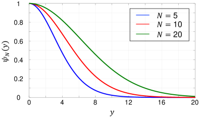
Figure 3: Plot of $\psi_{N}$.

The use of Berstein’s inequality (see, e.g., [40, Theorem 1.13]) or Theorem 6.5 of [41] for the tail bound (38) yields a simple but slightly conservative condition. In fact, if we use Berstein’s inequality, then (40) is replaced by the following simple condition:

$$\frac{\delta}{\epsilon}<\begin{cases}\dfrac{\Lambda}{4\ln(2/\zeta)}&\text{if $N\leq 2\ln(2/\zeta)$},\vspace{10pt}\\ \dfrac{\Lambda}{2\sqrt{2N\ln(2/\zeta)}}&\text{if $N>2\ln(2/\zeta)$}.\end{cases}$$ (41)

In Fig. 4, the circles and squares indicate the maximum value of $\delta/\epsilon$ satisfying (40) and (41) with $\zeta=0.01$ and $\Lambda=30$, respectively. As $\delta/\epsilon$ becomes large, we can choose smaller $\epsilon$ and larger $\delta$. This implies that it is more difficult (as $\epsilon$ becomes smaller) to distinguish the correct data and a wider range of data (as $\delta$ becomes larger). Note that (40) and (41) are obtained as sufficient conditions for ${\bf v}\sim\mathop{\rm Lap}(\delta/\epsilon)^{N}$ to satisfy (38). The diamonds in Fig. 4 are the maximum value of $\delta/\epsilon$ for which $\zeta$ is larger than the ratio of the number of samples ${\bf v}\sim\mathop{\rm Lap}(\delta/\epsilon)^{N}$ satisfying $\left|\sum_{i=1}^{N}v_{i}\right|>\Lambda$ to the total number of samples, $2\times 10^{5}$. We regard the diamonds as the exact value obtained numerically. Compared with this sampling approach, the computational cost of $\delta/\epsilon$ by the proposed condition (40) is very low. Moreover, we observe from Fig. 4 that the proposed condition (40) is less conservative than the conventional condition (41), in particular, for small $N$.

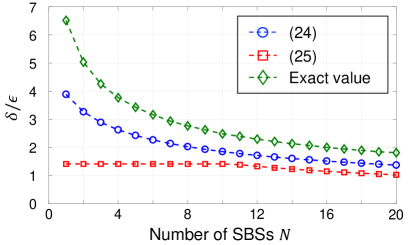
Figure 4: $\delta/\epsilon$ versus $N$.

Remark IV.4

Differential privacy has a limitation for intruders with knowledge of correlation between data when the data are continuously collected, as shown, e.g., in [42]. To apply the above analysis in such a situation, the central controller needs to detect packet sniffing so quickly that intruders can get at most “one-shot” data. Another possible approach is to apply data-releasing mechanisms against attackers with knowledge of data correlation proposed in [42], and we leave it for future studies.

V Performance Evaluation

In this section, we illustrate the effectiveness of the distributed control method through numerical simulations.

V-A Comparison with centralized control method

To evaluate robustness against masking noise, we compare the distributed control method with the centralized control method. From this comparison, we also analyze errors of the approximation methods proposed in Section III-A. Here we set the number of the SBSs to $N=4$. The reason for this small number of SBSs is that the centralized control method solves the original problem (9). The resulting worst-case complexity is at least $O(2^{N})$, and therefore the centralized control method is not applicable in the case of a large number of SBSs. In contrast, the distributed control method is dimension-free as mentioned in Remark III.1 and hence can deal with a larger number of SBSs. A simulation result of the distributed control method with $N=16$ will be given in Section V-B.

V-A1 Parameter settings

The parameters for simulations are listed in Table II. The service area of every SBS is a circle with radius 0.4 km, and hence the size is given by $A=(0.4)^{2}\pi$ km². Let the capacity and the initial energy of the battery in the SBSs be $X_{\max}=40$ kJ and $x_{i}[0]=30$ kJ, $i=1,\dots,4$, respectively. The sampling period is given by $h=300$ s. The power amplifier efficiency is set to $\gamma=0.32$. The MBS has a maximum capacity of $U_{\text{Macro}}=150$ users. The system powers are set to $s_{\text{active}}=1.5$ W in the active mode and to $s_{\text{sleep}}=0.5$ W in the sleep mode. The desired QoE value is given by $Q=4$, and for a data transmission model, the system noise, the packet size, and the path loss factor are set to $\sigma=-138.8$ dBm, $S=12000$ bit (1500 byte), and $Z=161.8296$ dBm, respectively, which are used in a standard LTE scenario studied in [31].

TABLE II: Parameter settings.

Parameter	Value		Parameter	Value
$N$	4		$S$	12000 bit
$A$	$(0.4)^{2}\pi\,\text{km}^{2}$		$\nu_{11},\nu_{21}$	60, 70 users
$X_{\max}$	40 kJ		$\nu_{12},\nu_{22}$	90, 80 users
$x_{i}[0]$	30 kJ		$\nu_{13},\nu_{23}$	70, 90 users
$\gamma$	0.32		$\nu_{14},\nu_{24}$	80, 60 users
$h$	300 s		$p_{1},p_{2}$	144, 174
$U_{\text{Marco}}$	150 users		$p_{3},p_{4}$	114, 144
$s_{\text{acitve}}$	1.5 W		$\lambda$	$5\times 10^{-5}$
$s_{\text{sleep}}$	0.5 W		$c$	0.1
$\sigma$	$-138.8$ dB		$u_{\text{thres}}$	0.1 W
$Z$	161.8296 dBm		$T$	20
$Q$	4		$\alpha^{[t]}$	$7/t$

We present two-day simulations of cell zooming. The number of users of the area of the $i$th SBS is given by

$$U_{i}[k]=\begin{cases}\nu_{1i}\exp\left(\frac{-(k-p_{i})^{2}}{10^{5}}\right)&\text{if $0\leq k<288$},\vspace{3pt}\\ \nu_{2i}\exp\left(\frac{-(k-p_{i}-288)^{2}}{10^{5}}\right)&\text{if $288\leq k\leq 576$}\end{cases}$$ (42)

for each $i=1,\dots,4$. Note that since $h=300$ s, it follows that $288h$ is $24$ hours. The numbers of users have the period of 24 hours and the peaks $\nu_{1i}$ and $\nu_{2i}$ at $k=p_{i}$ and $k=p_{i}+288$ on the first and second days, respectively. These parameters are set to $(\nu_{11},\nu_{21},p_{1})=(60,70,144)$, $(\nu_{12},\nu_{22},p_{2})=(90,80,174)$, $(\nu_{13},\nu_{23},p_{3})=(70,90,114)$, $(\nu_{14},\nu_{24},p_{4})=(80,60,144)$. Fig. 5 shows the number of users in the service area of each SBS.

The harvested power is set to

$$w_{i}[k]=\begin{cases}10\exp\left(\frac{-(k-144)^{2}}{5\times 10^{4}}\right)&\text{if $0\leq k<288$},\vspace{3pt}\\ 10\exp\left(\frac{-(k-432)^{2}}{5\times 10^{4}}\right)&\text{if $288\leq k\leq 576$}\end{cases}$$ (43)

for every $i=1,\dots,4$. The harvested power has the period of 24 hours and the peak $10$ W at noon, $k=144$ and $k=432$. The harvested power also has a bell-shaped curve similar to the numbers of users in Fig. 5.

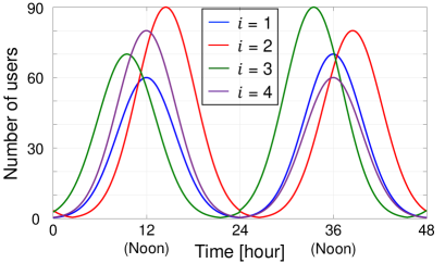
Figure 5: Numbers of users in service areas of SBSs.

The parameters of the proposed method are as follows. The weight $\lambda$ of the objective function is $\lambda=5\times 10^{-5}$. The parameters for the approximation techniques are given by $c=0.1$ and $u_{\textrm{thres}}=0.1$ W. The terminal step $T$ and the stepsize $\alpha^{[t]}$ of Algorithm 1 are $T=20$ and $\alpha^{[t]}=7/t$.

V-A2 Robustness of cell zooming against masking noise

In this section, we compare the numbers of users associated with the SBSs in the presence/absence of masking noise. This comparison verifies that the distributed control method, that is, Algorithm 1 and the formula (33), is more robust against masking noise than the centralized control method. Let each noise $v_{i}[k]$ be independently and identically distributed according the Laplace distribution $\mathop{\rm Lap}(\rho)$. Hence, for all $\epsilon,\delta>0$ satisfying $\delta/\epsilon=\rho$, the cell zooming method achieves $\epsilon$-differential privacy for $\delta$-adjacent pairs by the Laplace mechanism.

Fig. 6 plots the numbers of users associated with the SBSs, $\sum_{i=1}^{N}F\big{(}u_{i}[k],U_{i}[k]\big{)}$, in the noiseless case $\rho=0$ and the case $\rho=10$. In Fig. 7, we present the residual energy of the battery in each SBS in the case $\rho=10$. The centralized control case is given in Figs. 6(a) and 7(a), and the distributed control case is in Figs. 6(b) and 7(b).

From Figs. 6 and 7, we observe that the centralized control method is sensitive to masking noise, whereas in the distributed control case, the effect of masking noise appears only in short periods such as the interval $[31,34]$. This is because in the distributed control method, the objective function is not affected by the masking noise. Although the constraint [C5] is affected by the noise even in the distributed control case, this constraint is satisfied for all sufficiently large transmission powers. Moreover, the analysis in Section IV-B shows that the effect of the masking noise to the constraint becomes smaller as the transmission power increases. Hence the error of [C5] due to the masking noise does not change the optimal solution in the situation where the SBSs have plenty of energy. In the simulation of the distributed control case, the available energy of two SBSs $i=2,3$ is small in the interval $[31,34]$ as shown in Fig. 7(b), and hence we observe the noise effect in this interval in Fig. 6(b). The residual energy of the SBS $i=2$ is already depleted before the interval $[31,34]$. However, its effect is not seen in Fig. 6(b), because only a few users are active in the area of the SBS $i=2$ in the interval $[24,31]$ as shown in Fig. 5.

Moreover, Fig. 6 shows that in the noiseless case, the number of users by the distributed control method is almost the same as that by the centralized control method, although the approximate problem is solved in the distributed control case. This implies that the proposed approximation techniques have only small errors.

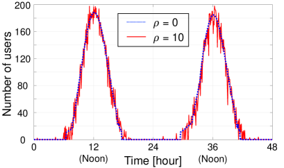
(a) Centralized control.

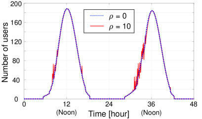
(b) Distributed control.

Figure 6: Numbers of users associated with SBSs in the cases $\rho=0,10$.

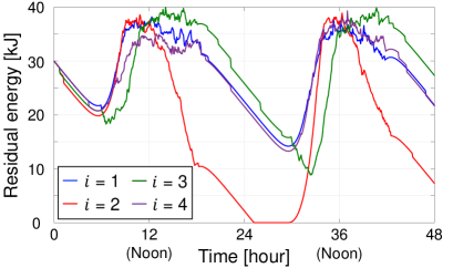
(a) Centralized control.

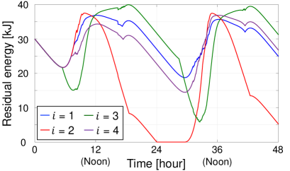
(b) Distributed control.

Figure 7: Residual energy of each SBS in the case $\rho=10$.

Fig. 8 plots control performances versus noise intensity. As control performances, we consider the energy efficiency over the two days, i.e.,

$$\frac{\text{(Total number of users associated with SBSs)}}{\text{(Total consumed energy [kJ])}}$$ (44)

in Fig. 8(a) and the average of the charging rate of the batteries, i.e.,

$$\frac{1}{577N}\sum_{k=0}^{576}\sum_{i=1}^{N}\frac{x_{i}[k]}{X_{\max}}$$ (45)

in Fig. 8(b). We compute the above criteria with $500$ samples of ${\bf v}\sim\mathop{\rm Lap}(\rho)^{N}$ for both the centralized and distributed control methods. As expected, in the noiseless case $\rho=0$, the performance of distributed control method is slightly worse than that of the centralized control method due to approximation errors. However, we see from Fig. 8 that the performance of the centralized control method becomes worse sharply as the intensity of masking noise increases. In contrast, the distributed control method is robust against masking noise, and in particular, its performance is not harmed by masking noise with small intensity.

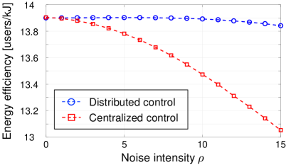
(a) Energy efficiency versus noise intensity.

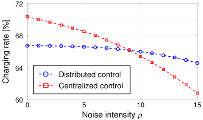
(b) Charging rate versus noise intensity.

Figure 8: Robustness against noise. For all $\epsilon,\delta>0$ satisfying $\delta/\epsilon=\rho$, the cell zooming method achieves $\epsilon$-differential privacy for $\delta$-adjacent pairs by the Laplace mechanism.

V-A3 Truncation and approximation errors

In this section, we investigate the following errors:

• the truncation error of Algorithm 1 due to the finiteness of the terminal step $T$;

• the approximation error due to the transformation of the original minimization problem (9) into the form of (18).

In the simulations, we consider the noiseless case, that is, $v_{i}[k]=0$ for every $i,k$.

Fig. 9 depicts the percent error due to truncation, i.e.,

$$100\times\frac{\sum_{i=1}^{N}\big{\|}u_{i}^{[T]}-u_{i}^{[30]}\big{\|}_{2}~{}\!/~{}\!\big{\|}u_{i}^{[30]}\big{\|}_{2}}{N},$$ (46)

for $1\leq T\leq 29$, where

$$\|u\|_{2}:=\sqrt{\sum_{k=0}^{576}\big{|}u[k]\big{|}^{2}}$$

for $u=\begin{bmatrix}u[0]&\cdots&u[576]\end{bmatrix}$ and $u_{i}^{[T]}$ is the transmission power $u_{i}$ obtained by Algorithm 1 and the formula (33) with the terminal step $T$. The transmission power computed in Algorithm 1 converges as $T\to\infty$, but this does not imply that the truncation error is monotonically decreasing with respect to $T$. Hence the truncation error temporarily increases at $T=5$ in Fig. 9. We see from Fig. 9 that for $T\geq 10$, the truncation error is sufficiently small. Since the data transfer time between SBSs and MBSs is at most a few milliseconds, the proposed method computes the transmission power sufficiently fast.

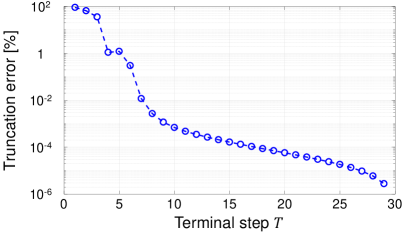
Figure 9: Truncation error versus terminal step $T$.

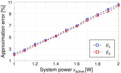
Figure 10: Approximation error versus system power $s_{\text{active}}$.

Fig. 10 plots the approximation error versus the system power in the active mode $s_{\text{active}}$. Let $u_{i}^{\text{exact}}$ be the transmission power of the $i$th SBS obtained by solving the minimization problem (9). Let $u_{i}^{\text{app}1}$ and $u_{i}^{\text{app}2}$ be the transmission powers of the $i$th SBS obtained by the Algorithm 1. To obtain $u_{i}^{\text{app}1}$, we use the formula (33) for the approximate solution of the minimization problem (26), while we compute the exact solution of the problem (26) for $u_{i}^{\text{app}2}$. The circles and the squires in Fig. 10 show the percent errors due to approximation, i.e,

$$E_{l}:=100\times\frac{\sum_{i=1}^{N}\big{\|}u_{i}^{\text{app}\hskip 1.0ptl}-u_{i}^{\text{exact}}\big{\|}_{2}~{}\!/~{}\!\big{\|}u_{i}^{\text{exact}}\big{\|}_{2}}{N}$$ (47)

for $l=1,2$, respectively. Fig. 10 indicates that the errors of the approximation techniques developed in Section III-A are quite small. We also observe that the approximation error becomes larger as $s_{\text{active}}$ increases. This is because the $\ell^{1}$ approximation of the $\ell^{0}$ norm in (15) yields larger errors as the difference of the system powers between the active and sleep modes, $s_{\text{active}}^{2}-s_{\text{sleep}}^{2}$, increases. Moreover, $u_{i}^{\text{app1}}$ has a slightly larger approximation error than $u_{i}^{\text{app2}}$, but the difference is negligibly small.

V-B Simulation of a large-sized cell network

Here we present a simulation result of a large-sized cell network. The number of the SBSs and the maximum capacity of the MBS are set to $N=16$ and $U_{\text{Macro}}=400$, respectively. The number of active users in the service area of each SBS is of the form (42), where the peaks $\nu_{1i}$, $\nu_{2i}$ and the peak time $p_{i}$ are chosen from the discrete uniform distribution on the sets $\{40,41,\dots,70\}$ and $\{114,115,\dots,174\}$, respectively. The harvested power is given by (43) for every SBS. Other parameters are the same as in Section V-A.

Fig. 11 shows the numbers of users accommodated by the SBSs, $\sum_{i=1}^{N}F\big{(}u_{i}[k],U_{i}[k]\big{)}$, for the noise intensities $\rho=0,10$. As in the case $N=4$, we observe the robustness of the proposed cell zooming method to the masking noise. The number of users fluctuates in some intervals in Fig. 11. The reason is the same as in the case $N=4$. In fact, the remaining energy of some SBSs is small in the intervals such as $[31,34]$. Since the simulation result of the SBS energy shows a trend almost identical to the case $N=4$, we omit it.

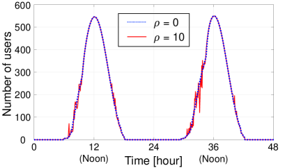
Figure 11: Numbers of users associated with SBSs in the case $N=16$.

VI Conclusion

We have proposed a cell zooming method with masked data for off-grid SBSs. We have formulated the minimization problem of cell zooming, in which the number of users associated with the SBSs and the available energy of the batteries in the SBSs are evaluated. To solve the minimization problem, the measurement data on the numbers of users in the service areas of the SBSs are required. We have preserved the confidential measurement data, by adding masking noise to them. We have developed a distributed cell zooming algorithm that is more robust to masking noise than the conventional centralized method. Although the originally formulated minimization problem is equivalent to a mixed integer nonlinear programing problem, the proposed algorithm computes its approximate solution with low computational complexity. In addition, we have analyzed the trade-off between confidentiality and optimization accuracy by using the notion of differential privacy. Our numerical results have shown that the distributed control method outperforms the centralized control method with respect to robustness against masking noise. Moreover, we have observed that the approximation error of the proposed method is quite small.

Appendix A Derivation of (9)

First, we approximate the objective function $P_{k}$ given in (7). The approximation techniques in 1) – 3) of Section III-A yield

$$\sum_{i=1}^{N}\Big{(}X_{\max}-\mathop{\rm sat}\big{(}x_{i}[k]-h(w_{i}[k]-u_{i}/\gamma-s_{i})\big{)}\Big{)}^{2}$$

$$~{}\approx\sum_{i=1}^{N}\Big{\{}(X_{\max}-x_{i}[k]-hw_{i}[k]+hu_{i}/\gamma)^{2}$$ (48)

$$\hskip 38.0pt+h^{2}\big{(}s_{\rm active}^{2}-s_{\rm sleep}^{2}\big{)}u_{i}+h^{2}s_{\rm sleep}^{2}$$

$$\hskip 38.0pt+2h(X_{\max}-x_{i}[k]-hw_{i}[k]+hu_{i}/\gamma)s_{i}[k-1]\Big{\}}.$$

Therefore, the objective function $P_{k}$ can be approximated as

$$P_{k}({\bf u},{\bf U})\approx\sum_{i=1}^{N}\Big{\{}f_{i,k}\big{(}u_{i},U_{i}[k]\big{)}+h^{2}s_{\rm sleep}^{2}$$

$$\qquad~{}~{}+2\lambda h\big{(}X_{\max}-x_{i}[k]-hw_{i}[k]\big{)}s_{i}[k-1]\Big{\}},$$ (49)

where the function $f_{i,k}$ is defined by (19b). Since the terms

$$h^{2}s_{\rm sleep}^{2},\quad 2\lambda h\big{(}X_{\max}-x_{i}[k]-hw_{i}[k]\big{)}s_{i}[k-1]$$ (50)

do not depend on the variables $u_{1},\dots,u_{N}$, it follows that minimizing the function in the right-hand side of (49) is equivalent to minimizing $\sum_{i=1}^{N}f_{i,k}(u_{i},U_{i}[k])$.

Next, we investigate the constraints [C3] and [C4]. The constraint [C3] is equivalent to

$$u_{i}\leq\gamma(x_{i}[k]/h+w_{i}[k]-s_{i}).$$ (51)

Since $u_{i}\geq 0$ and since $s_{i}=s_{\text{sleep}}$ is equivalent to $u_{i}=0$, we can rewrite (51) as

$$u_{i}\leq\max\big{\{}0,~{}\gamma(x_{i}[k]/h+w_{i}[k]-s_{\text{active}})\big{\}}.$$ (52)

Moreover, for $U_{i}[k]>0$, the constraint [C4] is equivalent to $u_{i}\leq r^{-\frac{10}{19}}.$ Hence, the constraints [C3] and [C4] can be reduced to $u_{i}\leq u_{i}^{\max}[k]$, where $u_{i}^{\max}[k]$ is defined by (19a).

Finally, if we define a function $g$ as in (19c), then $\sum_{i=1}^{N}g(u_{i},U_{i}[k])\leq 0$ if and only if [C5’] given in (17) holds. Thus, the minimization problem (9) is approximated by a minimization problem of the form (18).

Appendix B Proof of Theorem III.2

a) Define the nonlinear function $\Xi$ by

$$\Xi(u):=p_{1}u^{\frac{28}{19}}+p_{2}u^{\frac{10}{19}}+p_{3}u^{\frac{9}{19}}-p_{4}.$$ (53)

We will show that $\Xi(u)=0$ has a unique positive solution. Note that the coefficients $p_{1}$, $p_{2}$, and $p_{4}$ are non-negative but that $p_{3}$ may be negative. Let us first consider the case $p_{3}\geq 0$. In this case, $\Xi$ is monotonically increasing. Since $\Xi(0)=-p_{4}<0$, it follows that $\Xi(u)=0$ has a unique positive solution $u^{\mathop{\rm sol}}$.

Next, we consider the case $p_{3}<0$. The derivative $\Xi^{\prime}(u)$ is given by

$$\Xi^{\prime}(u)=\frac{28p_{1}u+10p_{2}u^{\frac{1}{19}}+9p_{3}}{19u^{\frac{10}{19}}}.$$ (54)

There exists a unique positive solution $u=\tilde{u}$ of $\Xi^{\prime}(u)=0$, and $\Xi$ has a minimum at $u=\tilde{u}$. Hence, there uniquely exists $u^{\mathop{\rm sol}}>0$ such that $\Xi(u^{\mathop{\rm sol}})=0$.

We prove that the solution $u^{*}$ of the minimization problem (26) is given by (28). Define the function $L(u)$ by

$$L(u) :=f(u,U)+\mu g(u,U+v)$$

$$=R_{1}\left(1-ru^{\frac{10}{19}}\right)^{2}+R_{2}\left(1-ru^{\frac{10}{19}}\right)$$ (55)

$$\qquad+\lambda(R_{3}+\beta_{1}u)^{2}+\beta_{2}u-V,$$

where

$$R_{1} :=U^{2},\quad R_{2}:=\mu(U+v),\quad R_{3}:=X_{\max}-x-hw$$ (56)

$$\beta_{1} :=\frac{h}{\gamma},\quad\beta_{2}:=\lambda h^{2}\left(s_{\rm active}^{2}-s_{\rm sleep}^{2}+\frac{2s[k-1]}{\gamma}\right)$$ (57)

$$V :=\frac{\mu(1-c)U_{\text{Macro}}}{N}.$$ (58)

Then we obtain $L^{\prime}(u)=u^{-\frac{9}{19}}\Xi(u)$, where $\Xi$ is defined as in (53). Since $\Xi(u)<0$ for all $u<u^{\mathop{\rm sol}}$ and $\Xi(u)>0$ for all $u>u^{\mathop{\rm sol}}$, it follows that $\min_{u\geq 0}L(u)=L(u^{\mathop{\rm sol}}).$ If $u^{\mathop{\rm sol}}>u^{\max}$, then $L$ is monotonically decreasing on $[0,u^{\max}]$. Thus, the solution $u^{*}$ of the minimization problem (26) is given by (28).

b) The second assertion follows from an argument similar to that in the proof of Theorem 3 of [12]. Suppose that $p_{3}\geq 0$. Define

$$\Xi_{1}(u) :=p_{1}u^{\frac{27}{19}}+p_{2}u^{\frac{9}{19}}+p_{3}u^{\frac{9}{19}}-p_{4}$$ (59)

$$\Xi_{2}(u) :=p_{1}u^{\frac{30}{19}}+p_{2}u^{\frac{10}{19}}+p_{3}u^{\frac{10}{19}}-p_{4}.$$ (60)

Note that $\Xi_{1}$ and $\Xi_{2}$ are in the form of a cubic polynomial

$$p_{1}\chi^{3}+(p_{2}+p_{3})\chi-p_{4}$$

with $\chi=u^{\frac{9}{19}}$ and $\chi=u^{\frac{10}{19}}$, respectively. Since $\Xi_{1}(0)=\Xi_{2}(0)=-p_{4}<0$ and since $\Xi_{1}$ and $\Xi_{2}$ are monotonically increasing, $\Xi_{1}(u)=0$ and $\Xi_{2}(u)=0$ have unique positive solutions $u_{1}^{\mathop{\rm sol}}$ and $u_{2}^{\mathop{\rm sol}}$, respectively. We obtain

$$\Xi(u)-\Xi_{1}(u) =p_{1}\Big{(}u^{\frac{28}{19}}-u^{\frac{27}{19}}\Big{)}+p_{2}\Big{(}u^{\frac{10}{19}}-u^{\frac{9}{19}}\Big{)}$$ (61)

$$\Xi_{2}(u)-\Xi(u) =p_{1}\Big{(}u^{\frac{30}{19}}-u^{\frac{28}{19}}\Big{)}+p_{3}\Big{(}u^{\frac{10}{19}}-u^{\frac{9}{19}}\Big{)},$$ (62)

and it follows from $p_{1}>0$ and $p_{2},p_{3}\geq 0$ that

$$\begin{cases}\Xi_{2}(u)<\Xi(u)<\Xi_{1}(u)&\text{if $0<u<1$},\\ \Xi_{1}(u)<\Xi(u)<\Xi_{2}(u)&\text{if $u>1$.}\end{cases}$$ (63)

Moreover, $\Xi_{1}(1)=\Xi(1)=\Xi_{2}(1)$. Hence

$$\begin{cases}u_{1}^{\mathop{\rm sol}}\leq u^{\mathop{\rm sol}}\leq u_{2}^{\mathop{\rm sol}}&\text{if $u_{2}^{\mathop{\rm sol}}\leq 1$},\\ u_{2}^{\mathop{\rm sol}}\leq u^{\mathop{\rm sol}}\leq u_{1}^{\mathop{\rm sol}}&\text{if $u_{2}^{\mathop{\rm sol}}>1$.}\end{cases}$$ (64)

The unique positive solution of the cubic equation

$$p_{1}\chi^{3}+(p_{2}+p_{3})\chi-p_{4}=0$$

is given by (31). Together with this, (64) yields (30). $\blacksquare$

Appendix C Proof of Proposition IV.3

We use a tail bound for the sum of independent and identically distributed Laplace random variables in the proof of Proposition IV.3. The following tail bound can be obtained by a standard technique based on the Chernoff bound (see, e.g., [40, Section 1.2]), but we give the proof for completeness.

Lemma A

For all $\rho>0$ and $\Lambda>0$, independent and identically distributed random variables $W_{1},\dots,W_{N}\sim\mathop{\rm Lap}(\rho)$ satisfy

$$\textrm{{\em P}}\left(\left|\sum_{i=1}^{N}W_{i}\right|>\Lambda\right)\leq 2\psi_{N}(\Lambda/\rho),$$ (65)

where $\psi_{N}$ is defined by (39).

Proof: It is enough to show that (65) holds for $\rho=1$. We obtain the general case $\rho\not=1$ by replacing $W_{i}$ and $\Lambda$ by $W_{i}/\rho\sim\mathop{\rm Lap}(1)$ and $\Lambda/\rho$, respectively.

For each $i=1,\dots,N$, the moment generating function of $W_{i}\sim\mathop{\rm Lap}(1)$ is given by

$$\textrm{E}\big{[}e^{W_{i}z}\big{]}=\frac{1}{1-z^{2}}\qquad\forall z\in(-1,1).$$ (66)

Using the Chernoff bound, we obtain

$$\textrm{P}\left(\sum_{i=1}^{N}W_{i}>\Lambda\right) \leq e^{-\Lambda z}\prod_{i=1}^{N}\textrm{E}\big{[}e^{W_{i}z}\big{]}$$ (67)

$$=\frac{e^{-\Lambda z}}{(1-z^{2})^{N}}=:\phi(z)$$ (68)

for every $z\in(0,1)$.

We next investigate $\inf_{0<z<1}\phi(z)$. Define

$$\Phi(z):=\ln\phi(z)=-\Lambda z-N\ln\big{(}1-z^{2}\big{)}.$$

Since

$$\Phi^{\prime}(z)=-\Lambda+\frac{2Nz}{1-z^{2}},$$ (69)

it follows that $\inf_{0<z<1}\Phi(z)=\Phi\big{(}\varpi(\Lambda)\big{)}$, where

$$\varpi(\Lambda):=\frac{\sqrt{N^{2}+\Lambda^{2}}-N}{\Lambda}\in(0,1)\qquad\forall N\in\mathbb{N}.$$ (70)

The increasing property of logarithmic functions yields

$$\inf_{0<z<1}\phi(z)=\phi\big{(}\varpi(\Lambda)\big{)}=\psi_{N}(\Lambda),$$ (71)

where $\psi_{N}$ is defined by (39). We obtain the same bound for

$$\textrm{P}\left(\sum_{i=1}^{N}W_{i}<-\Lambda\right).$$

Thus, (65) holds. $\Box$

Proof of Proposition IV.3: By Lemma A, we obtain

$$\textrm{P}\left(\left|\sum_{i=1}^{N}W_{i}\right|>\Lambda\right)<\zeta$$

for $W_{i}\sim\mathop{\rm Lap}(\delta/\epsilon)$, $1\leq i\leq N$, if $2\psi_{N}(\epsilon\Lambda/\delta)<\zeta$. The $\epsilon$-differential privacy of the mechanism ${\bf\Theta}({\bf U},{\bf v})={\bf U}+{\bf v}$ for $\delta$-adjacent pairs immediately follows from the Laplace mechanism for $\epsilon$-differential privacy; see [29, Theorem 3.6] and [39, Section 5.1].

To see that the function $\psi_{N}$ is decreasing on $(0,\infty)$, we obtain

$$\psi_{N}^{\prime}(y) =\frac{y^{2N-1}e^{N-\sqrt{y^{2}+N^{2}}}\big{(}2N\sqrt{{y^{2}+N^{2}}}-y^{2}-2N^{2}\big{)}}{(2N)^{N}\big{(}\sqrt{y^{2}+N^{2}}-N\big{)}^{N+1}}.$$

Since

$$\big{(}2N\sqrt{{y^{2}+N^{2}}}\big{)}^{2}-\big{(}y^{2}+2N^{2}\big{)}^{2}=-y^{4},$$ (72)

it follows that $\psi_{N}^{\prime}(y)<0$ for all $y\in(0,\infty)$. Hence $\psi_{N}$ is decreasing on $(0,\infty)$. This completes the proof. $\blacksquare$

References

- [1] A. P. Couto da Silva, D. Renga, M. Meo, and M. Ajmone Marsan, “The impact of quantization on the design of solar power systems for cellular base stations,” IEEE Trans. Green Commun. Netw., vol. 2, no. 1, pp. 260–274, Mar. 2018.
- [2] M. S. Hossain, A. Jahid, K. Z. Islam, and M. F. Rahman, “Solar PV and biomass resources-based sustainable energy supply for off-grid cellular base stations,” IEEE Access, vol. 8, pp. 53 817–53 840, 2020.
- [3] H. Ko, S. Pack, and V. C. M. Leung, “Energy utilization-aware operation control algorithm in energy harvesting base stations,” IEEE Internet of Things J., vol. 6, no. 6, pp. 10 824–10 833, Dec. 2019.
- [4] G. Piro, M. Miozzo, G. Forte, N. Baldo, L. A. Grieco, G. Boggia, and P. Dini, “HetNets powered by renewable energy sources: Sustainable next-generation cellular networks,” IEEE Internet Comput., vol. 17, no. 1, pp. 32–39, Jan. 2013.
- [5] L. An, T. Zhang, and C. Feng, “Joint optimization for base station density and user association in energy-efficient cellular networks,” in Proc. Int. Symp. Wireless Pers. Multimedia Commun. (WPMC), Sept. 2014, pp. 85–90.
- [6] C.-Y. Chang, K.-L. Ho, W. Liao, and D.-S. Shiu, “Capacity maximization of energy-harvesting small cells with dynamic sleep mode operation in heterogeneous networks,” in Proc. IEEE Int. Conf. Commun. (ICC), June 2014, pp. 2690–2694.
- [7] S. Maghsudi and E. Hossain, “Distributed user association in energy harvesting small cell networks: A probabilistic bandit model,” IEEE Trans. Wireless Commun., vol. 16, no. 3, pp. 1549–1563, Mar. 2017.
- [8] ——, “Distributed user association in energy harvesting small cell networks: An exchange economy with uncertainty,” IEEE Trans. Green Commun. Netw., vol. 1, no. 3, pp. 294–308, Sept. 2017.
- [9] K.-H. Liu and T.-Y. Yu, “Performance of off-grid small cells with non-uniform deployment in two-tier HetNet,” IEEE Trans. Wireless Commun., vol. 17, no. 9, pp. 6135–6148, Sept. 2018.
- [10] S. Zhang, N. Zhang, S. Zhou, J. Gong, Z. Niu, and X. Shen, “Energy-aware traffic offloading for green heterogeneous networks,” IEEE J. Sel. Areas Commun., vol. 34, no. 5, pp. 1116–1129, May 2016.
- [11] H. Jiang, S. Yi, L. Wu, H. Leung, Y. Wang, X. Zhou, Y. Chen, and L. Yang, “Data-driven cell zooming for large-scale mobile networks,” IEEE Netw. Service Manag., vol. 15, no. 1, pp. 156–168, Mar. 2018.
- [12] M. Wakaiki, K. Suto, K. Koiwa, K. Liu, and T. Zanma, “A control-theoretic approach for cell zooming of energy harvesting small cell networks,” IEEE Trans. Green Commun. Netw., vol. 3, no. 2, pp. 329–342, June 2018.
- [13] V. Chamola, B. Krishnamachari, and B. Sikdar, “Green energy and delay aware downlink power control and user association for off-grid solar-powered base stations,” IEEE Syst. J., vol. 12, no. 3, pp. 2622–2633, Sept. 2018.
- [14] G. Lee, W. Saad, M. Bennis, A. Mehbodniya, and F. Adachi, “Online ski rental for ON/OFF scheduling of energy harvesting base stations,” IEEE Trans. Wireless Commun., vol. 16, no. 5, pp. 2976–2990, May 2017.
- [15] A. Alqasir and A. Kamal, “Cooperative small cell HetNets with dynamic sleeping and energy harvesting,” IEEE Trans. Green Commun. Netw., vol. 4, no. 3, pp. 774–782, Sept. 2020.
- [16] M. Miozzo, N. Piovesan, and P. Dini, “Coordinated load control of renewable powered small base stations through layered learning,” IEEE Trans. Green Commun. Netw., vol. 4, no. 1, pp. 16–30, Mar. 2020.
- [17] K. Suto, H. Nishiyama, N. Kato, and T. Kuri, “Model predictive joint transmit power control for improving system availability in energy-harvesting wireless mesh networks,” IEEE Commun. Lett., vol. 22, no. 10, pp. 2112–2115, Oct. 2018.
- [18] H. Wu, X. Tao, N. Zhang, D. Wang, S. Zhang, and X. Shen, “On base station coordination in cache- and energy harvesting-enabled HetNets: A stochastic geometry study,” IEEE Trans. Commun., vol. 66, no. 7, pp. 3079–3091, July 2018.
- [19] Y.-J. Ku, P.-H. Chiang, and S. Dey, “Real-time QoS optimization for vehicular edge computing with off-grid roadside units,” IEEE Trans. Veh. Technol., vol. 69, no. 10, pp. 11 975–11 991, Oct. 2020.
- [20] N. Piovesan, D. López-Pérez, M. Miozzo, and P. Dini, “Joint load control and energy sharing for renewable powered small base stations: A machine learning approach,” IEEE Trans. Green Commun. Netw., vol. 5, no. 1, pp. 512–525, Mar. 2021.
- [21] Y. Sekimoto, R. Shibasaki, H. Kanasugi, T. Usui, and Y. Shimazaki, “PFlow: Reconstructing people flow recycling large-scale social survey data,” IEEE Pervasive Comput., vol. 10, no. 4, pp. 27–35, Apr. 2011.
- [22] E. Toch, B. Lerner, E. Ben-Zion, and I. Ben-Gal, “Analyzing large-scale human mobility data: A survey of machine learning methods and applications,” Knowl. Inf. Syst., vol. 58, no. 3, pp. 501–523, Mar. 2019.
- [23] S. Ansari, S. G. Rajeev, and H. S. Chandrashekar, “Packet sniffing: A brief introduction,” IEEE Potentials, vol. 21, no. 5, pp. 17–19, Jan. 2003.
- [24] L. F. Sikos, “Packet analysis for network forensics: A comprehensive survey,” Forensic Sci. Int., Digit. Invest., vol. 32, Art. no. 200892, Mar. 2020.
- [25] D. P. Bertsekas, Nonlinear Programming, 2nd ed. Belmont, MA: Athena Scientific, 1999.
- [26] B. Yang and M. Johansson, “Distributed optimization and games: A tutorial overview,” in Networked Control Systems, A. Bemporad, M. Heemels, and M. Johansson, Eds. London: Springer, 2010, pp. 109–148.
- [27] T. Yang, X. Yi, J. Wu, Y. Yuan, D. Wu, Z. Meng, Y. Hong, H. Wang, Z. Lin, and K. H. Johansson, “A survey of distributed optimization,” Annu. Rev. Control, vol. 47, pp. 278–305, 2019.
- [28] D. L. Donoho, “Compressed sensing,” IEEE Trans. Inf. Theory, vol. 52, no. 4, pp. 1289–1306, Apr. 2006.
- [29] C. Dwork and A. Roth, “The algorithmic foundations of differential privacy,” Found. Trands Theor. Comput. Sci., vol. 9, no. 3–4, pp. 211–407, Aug. 2014.
- [30] M. Wakaiki, K. Suto, and I. Masubuchi, “Privacy-preserved cell zooming with distributed optimization in green networks,” in Proc. IEEE 90th Veh. Technol. Conf. (VTC-Fall), Sept. 2019, pp. 1–5.
- [31] K. Suto, H. Nishiyama, and N. Kato, “Postdisaster user location maneuvering method for improving the QoE guaranteed service time in energy harvesting small cell networks,” IEEE Trans. Veh. Technol., vol. 66, no. 10, pp. 9410–9420, Oct. 2017.
- [32] K. Wada and K. Sakurama, “Privacy masking for distributed optimization and its application to demand response in power grids,” IEEE Trans. Ind. Electron., vol. 64, no. 6, pp. 5118–5128, June 2017.
- [33] N. Hayashi and M. Nagahara, “Consensus-based distributed event-triggered sparse modeling,” in Proc. SICE Annu. Conf. 2018, Sept. 2018, pp. 1801–1805.
- [34] M. Nagahara, Sparsity Methods for Systems and Control. Hanover, MA: Now Publishers, 2020.
- [35] S.-S. Ho and S. Ruan, “Preserving privacy for interesting location pattern mining from trajectory data,” Trans. Data Privacy, vol. 6, no. 1, pp. 87–106, Apr. 2013.
- [36] X. Liao, P. Srinivasan, D. Formby, and R. A. Beyah, “Di-PriDA: Differentially private distributed load balancing control for the smart grid,” IEEE Trans. Depend. Secure Comput., vol. 16, no. 6, pp. 1026–1039, Nov./Dec. 2019.
- [37] M. U. Hassan, M. H. Rehmani, and J. Chen, “Differential privacy techniques for cyber physical systems: A survey,” IEEE Commun. Surveys Tuts., vol. 22, no. 1, pp. 746–789, 1st Quart. 2020.
- [38] E. Nozari, P. Tallapragada, and J. Cortés, “Differentially private average consensus: Obstructions, trade-offs, and optimal algorithm design,” Automatica, vol. 81, pp. 221–231, July 2017.
- [39] S. Weerakkody, O. Ozel, Y. Mo, and B. Sinopoli, “Resilient control in cyber-physical systems: Countering uncertainty, constraints, and adversarial behavior,” Found. Trends Syst. Control, vol. 7, no. 1–2, pp. 1–252, Dec. 2019.
- [40] P. Rigollet and J.-C. Hütter, High Dimensional Statistics. MIT Lecture Notes. Retrieved Oct. 20, 2021, from http://www-math.mit.edu/~rigollet/PDFs/RigNotes17.pdf.
- [41] A. Gupta, A. Roth, and J. Ullman, “Iterative constructions and private data release,” Proc. 9th IACR Theory Cryptogr. Conf. (TCC), pp. 339–356, Mar. 2012.
- [42] Y. Cao, M. Yoshikawa, Y. Xiao, and L. Xiong, “Quantifying differential privacy in continuous data release under temporal correlations,” IEEE Trans. Knowl. Data Eng., vol. 31, no. 7, pp. 1281–1295, July 2019.