Sinusoidal Flow: A Fast Invertible Autoregressive Flow

Abstract

Normalising flows offer a flexible way of modelling continuous probability distributions. We consider expressiveness, fast inversion and exact Jacobian determinant as three desirable properties a normalising flow should possess. However, few flow models have been able to strike a good balance among all these properties. Realising that the integral of a convex sum of sinusoidal functions squared leads to a bijective residual transformation, we propose Sinusoidal Flow, a new type of normalising flows that inherits the expressive power and triangular Jacobian from fully autoregressive flows while guaranteed by Banach fixed-point theorem to remain fast invertible and thereby obviate the need for sequential inversion typically required in fully autoregressive flows. Experiments show that our Sinusoidal Flow is not only able to model complex distributions, but can also be reliably inverted to generate realistic-looking samples even with many layers of transformations stacked.

1 Introduction

Estimating arbitrarily complex probability distributions from data is a critical task in machine learning, as an accurate specification of the underlying probabilistic model allows us to perform useful statistical computations such as generating samples or making inferences. Among all the tools available, normalising flows (Tabak and Turner, 2013; Rezende and Mohamed, 2015) appear as a highly flexible method for modelling continuous probability distributions by constructing a differentiable, bijective transformation $T:\mathcal{Z}\subseteq\mathbb{R}^{D}\mapsto\mathbb{R}^{D}$ that transforms a random vector $\mathbf{z}\in\mathbb{R}^{D}$, whose distribution is known and supported on $\mathcal{Z}$, to the random vector $\mathbf{x}\in\mathbb{R}^{D}$ whose distribution is to be estimated. The distribution of $\mathbf{z}$ is usually chosen to be a simple one, such as the standard multivariate Gaussian distribution:

$$\mathbf{x}=T\left(\mathbf{z}\right),\;\mathrm{where}\;\mathbf{z}\sim p_{\mathbf{z}}\left(\mathbf{z}\right)=\mathcal{N}\left(\mathbf{z}\mid\mathbf{0},\mathbf{I}\right)$$ (1)

The change-of-variable formula for probability density functions (Casella and Berger, 2001) then allows the unknown density $p_{\mathbf{x}}$ to be specified in terms of the known density $p_{\mathbf{z}}$:

$$p_{\mathbf{x}}\left(\mathbf{x}\right)=p_{\mathbf{z}}\left(T^{-1}\left(\mathbf{x}\right)\right)\cdot\lvert\mathrm{det}\,\mathbf{J}_{T^{-1}}\left(\mathbf{x}\right)\rvert$$ (2)

where $\mathbf{J}_{T^{-1}}\left(\mathbf{x}\right)$ is the $D\times D$ Jacobian matrix of the inverse transformation $T^{-1}$. Depending on how $T^{-1}$ is constructed, normalising flows can be broadly categorised into discrete-time flows and continuous-time flows (Papamakarios et al., 2019).

Discrete-time flows feature a decomposition of $T^{-1}$ into a finite number of simpler transformations:

$$T^{-1} =T^{-1}_{L}\circ T^{-1}_{L-1}\circ\cdots\circ T^{-1}_{1}$$ (3)

$$\mathrm{det}\,\mathbf{J}_{T^{-1}} =\mathrm{det}\,\mathbf{J}_{T^{-1}_{L}}\times\mathrm{det}\,\mathbf{J}_{T^{-1}_{L-1}}\times\cdots\times\mathrm{det}\,\mathbf{J}_{T^{-1}_{1}}$$ (4)

where each constituent transformation $T_{l}^{-1}$ can be implemented as a neural network layer and the calculation of the overall Jacobian determinant can be decentralised to each layer. Depending on how each constituent transformation is constructed, discrete-time flows can be further divided into fully autoregressive, partially autoregressive and residual flows (Papamakarios et al., 2019), which we describe in Section 2, along with continuous-time flows.

We think the following three properties, among others, desirable for normalising flows.

Expressiveness: how well a normalising flow can represent an arbitrary probability distribution. The expressive power of a normalising flow largely depends on how the transformation $T^{-1}$ (or equivalently, $T$) is constructed. Models that advocate strong dependency among the components of $\mathbf{x}$, such as fully autoregressive flows and residual flows, appear to exhibit strong expressive power as well. In fact, fully autoregressive flows are shown to be universal approximators under mild assumptions about $p_{\mathbf{x}}$ (Papamakarios et al., 2019), in that they can accurately represent any probability distributions given a transformation $T^{-1}$ with sufficient capacity.

Fast inversion: whether a normalising flow can be inverted computationally efficiently. The formulation of normalising flows in Equation 2 is well-suited for density estimation; however, to generate samples from $p_{\mathbf{x}}$ we would need to invert $T^{-1}$ to obtain $T$. Certainly, we can always invert any differentiable, theoretically invertible functions using a common root-finding algorithm, such as bisection or Newton’s method with a quadratic convergence rate, but we are interested in whether we can build normalising flows with an analytic inverse or with an even faster numerical inversion procedure that is also less sensitive to the choice of starting points. Due to the autoregressive dependency imposed on $\mathbf{x}$, fully autoregressive flows in general have to be inverted sequentially, one component at a time; moreover, depending on how each constituent transformation $T_{l}^{-1}$ is implemented component-wise, there may or may not exist a faster, more reliable inversion procedure than the Newton’s method. Partially autoregressive flows exchange some autoregressiveness for analytic invertibility at the cost of reduced expressive power. However, faster numerical inversion procedures do exist for residual flows and continuous-time flows, which we describe in Section 2.

Exact Jacobian determinant: whether the $\mathrm{det}\,\mathbf{J}_{T^{-1}}\left(\mathbf{x}\right)$ term in Equation 2 can be calculated exactly and efficiently. We can always compute the full Jacobian matrix of any neural network layer and its determinant at a cost of $\mathcal{O}\left(D^{3}\right)$, which is however intractable for very large $D$ as often seen in images or videos. So one of the focuses of previous work has been designing special architectures for the transformation $T^{-1}$ so that the Jacobian determinant can be either calculated exactly or estimated efficiently, both at a cost no more than $\mathcal{O}\left(D\right)$. Autoregressive flows feature a triangular Jacobian matrix at each layer whose determinant can be calculated exactly and efficiently by design. However, the Jacobian determinant for residual flows and continuous-time flows in general needs to be estimated or computed exactly at a cost slightly higher than $\mathcal{O}\left(D\right)$.

Table 1 summarises our best evaluation of some selected autoregressive, residual and continuous-time flows against the three desirable properties we propose. To the best of our knowledge, few normalising flows seem to have claimed excellence in all three dimensions. Fully autoregressive flows would have so if only they were as efficiently invertible as residual flows, whereas residual flows would have so if only they were made autoregressive to allow exact Jacobian determinant calculation. As we show in Section 3, our proposed Sinusoidal Flow is simultaneously a fully autoregressive flow and a residual flow, which strikes a good balance among all the three desirable properties.

Table 1: Evaluation of selected normalising flows against the three desirable properties we propose. The ratings for expressiveness represent our best subjective assessment on each method primarily based on the objective measures (if available) shown in Table 3. We understand that different normalising flows have different primary use cases. Normalising flows with convolutional architectures such as Glow (Kingma and Dhariwal, 2018), MaCow (Ma et al., 2019) and MintNet (Song et al., 2019) are better at modelling images. The ratings would have been different should we refer to a different objective measure.

Method	Expressiveness	Fast Inversion	Exact Jacobian Det.
Fully Autoregressive Flow
MAF (Papamakarios et al., 2017)		$\times$	$\surd$
NAF (Huang et al., 2018)		$\times$	$\surd$
B-NAF (De Cao et al., 2020)		$\times$	$\surd$
SOS (Jaini et al., 2019)		$\times$	$\surd$
UMNN-MAF (Wehenkel and Louppe, 2019)		$\times$	$\surd$
RQ-NSF(AR) (Durkan et al., 2019)		$\times$	$\surd$
Partially Autoregressive Flow
RealNVP (Dinh et al., 2017)		$\surd$	$\surd$
Glow (Kingma and Dhariwal, 2018)		$\surd$	$\surd$
RQ-NSF(C) (Durkan et al., 2019)		$\surd$	$\surd$
Residual Flow
i-ResNet (Behrmann et al., 2019)		$\surd$	$\times$
Continuous-time Flow
FFJORD (Grathwohl et al., 2019)		$\surd$	$\times$
Sinusoidal Flow (Ours)		$\surd$	$\surd$

2 Related Work

In this section, we review and analyse previous architectures of normalising flows related to our work, particularly with respect to the three desirable properties we propose.

2.1 Autoregressive Flows

Autoregressive flows are usually specified in terms of a “transformer” $\tau$ acting on each component of the input vector and a “conditioner” $c_{i}$ that computes the parameters of the transformer autoregressively based on the input. In other words, each constituent transformation $T_{l}^{-1}$ in Equation 3 consists of the following transformation for each component of the input $\mathbf{z}^{l-1}$ and the corresponding output $\mathbf{z}^{l}$ at layer $l$, if we let $\mathbf{x}=\mathbf{z}^{0}$ and $\mathbf{z}=\mathbf{z}^{L}$:

$$z_{i}^{l}=\tau(z_{i}^{l-1};\mathbf{h}_{i}),\;\text{where}\;\mathbf{h}_{i}=c_{i}(\mathbf{z}_{<i}^{l-1})$$ (5)

The conditioner $c_{i}$ for the $i$-th input component takes all the components preceding the $i$-th and computes the parameters $\mathbf{h}_{i}$ for the transformer $\tau$. Sometimes though, it may be desirable for the conditioner $c_{i}$ to output parameters that are independent from the input, in which case we shall call the conditioner an independent conditioner.

2.1.1 The Transformers

The transformer $\tau$ can assume many functional forms, so long as it is differentiable and invertible. Usually it is designed as a strictly monotonic function, since strict monotonicity implies invertibility. Popular choices include affine transformers (Dinh et al., 2015, 2017; Kingma et al., 2016; Papamakarios et al., 2017; Kingma and Dhariwal, 2018), neural transformers (Huang et al., 2018; Ho et al., 2019; De Cao et al., 2020), spline-based transformers (Müller et al., 2019; Durkan et al., 2019) and integration-based transformers (Jaini et al., 2019; Wehenkel and Louppe, 2019).

The design of the transformers greatly affects the availability of efficient inversion procedures. More complex transformers are usually accompanied by a less efficient inversion procedure, but less complex transformers usually come at a cost of reduced expressive power. For example, the neural network backbone in NAF (Huang et al., 2018), B-NAF (De Cao et al., 2020) and UMNN-MAF (Wehenkel and Louppe, 2019) is shown to be very powerful, yet no faster inversion procedures other than the general bisection or Newton’s method are proposed by the authors. On the other hand, IAF (Kingma et al., 2016) and MAF (Papamakarios et al., 2017) employ trivially invertible affine transformers but are less expressive than those using neural transformers.

2.1.2 The Conditioners

The fundamental impediment to autoregressive flows’ efficient inversion lies in their characteristic autoregressive dependency, which is directly related to the design of the conditioners.

Fully autoregressive flows are equipped with conditioners that impose the fullest possible autoregressive dependency on the parameters $\mathbf{h}_{i}$ of each transformer. Each $\mathbf{h}_{i}$ depends on all preceding input components $\mathbf{z}_{<i}^{l-1}$ and each input component $z_{i}^{l-1}$ is non-trivially transformed by a conditional transformer $\tau\left(\cdot\;;\mathbf{h}_{i}\right)$. Popular choices for the conditioner include masked feed-forward networks from MADE (Germain et al., 2015), as used in IAF (Kingma et al., 2016), MAF (Papamakarios et al., 2017), B-NAF (De Cao et al., 2020), SOS (Jaini et al., 2019), RQ-NSF(AR) (Durkan et al., 2019) and UMNN-MAF (Wehenkel and Louppe, 2019), and masked convolutional networks, as used in MaCow (Ma et al., 2019) and MintNet (Song et al., 2019). The fully autoregressive dependency necessitates a sequential inversion: before inverting ${z}_{i}^{l}$ at layer $l$, all $\mathbf{z}_{<i}^{l-1}$ must first be recursively recovered from $\mathbf{z}_{<i}^{l}$ so that the conditioner $c_{i}$ can return the parameters of $\tau$, followed by a possibly non-trivial inversion procedure if $\tau$ is not so simple as an affine transformer.

Partially autoregressive flows offer an analytic inverse in place of sequential inversion by imposing autoregressive dependency on only part of the input. Specifically, at each layer, half of the input is left unchanged and is used by a shared conditioner to produce the parameters of the individual transformers for the other half of the input:

$$\begin{cases}z^{l}_{i}=z^{l-1}_{i}&\forall i\leq\lfloor D/2\rfloor\\ z^{l}_{i}=\tau(z^{l-1}_{i};\mathbf{h}_{i})&\forall i>\lfloor D/2\rfloor,\;\text{where}\;\left[\mathbf{h}_{\lfloor D/2\rfloor+1},\dots,\mathbf{h}_{D}\right]=c\left(\mathbf{z}^{l-1}_{i\leq\lfloor D/2\rfloor}\right)\end{cases}$$ (6)

This special architecture is also known as coupling layers. If the transformer $\tau$ is analytically invertible, then the entire flow is analytically invertible, as in NICE (Dinh et al., 2015), RealNVP (Dinh et al., 2017), Glow (Kingma and Dhariwal, 2018) and RQ-NSF(C) (Durkan et al., 2019). However, the analytic invertibility comes at a cost of reduced expressive power in general compared to their fully autoregressive counterparts; nevertheless, the use of multi-scale convolutional architectures makes them more suitable for modelling images.

In short, while inducing strong expressive power, fully autoregressive dependency greatly limits the availability of efficient inversion procedures for fully autoregressive flows. Partially autoregressive flows bypass the limitation at the expense of expressiveness. Both of them, however, feature a triangular Jacobian at each layer whose determinant can be calculated exactly and efficiently, thanks to the autoregressive dependency.

2.2 Residual Flows

In residual flows, each constituent transformation $T_{l}^{-1}$ in Equation 3 closely resembles a residual network (He et al., 2016):

$$\mathbf{z}^{l}=T_{l}^{-1}(\mathbf{z}^{l-1})=\mathbf{z}^{l-1}+f(\mathbf{z}^{l-1};\phi)$$ (7)

which can be made invertible with a special choice of $f$.

One possible design is constraining $f$ to be Lipschitz continuous with a Lipschitz constant $0\leq M<1$, so that $f$ becomes a contraction mapping. As noted in Behrmann et al. (2019), the Banach fixed-point theorem guarantees that every contraction mapping has a unique fixed point, which gives rise to a very efficient inversion procedure for contractive residual flows. As Papamakarios et al. (2019) shows, if $f$ is a contraction mapping, then the function $F\left(\mathbf{\hat{z}}\right)=\mathbf{z}^{l}-f\left(\mathbf{\hat{z}};\phi\right)$ is also a contraction mapping with a unique fixed point $\mathbf{z}^{\ast}$:

$$F(\mathbf{z}^{\ast})=\mathbf{z}^{l}-f\left(\mathbf{z}^{\ast};\phi\right)=\mathbf{z}^{\ast}$$ (8)

which implies $\mathbf{z}^{l}=T_{l}^{-1}\left(\mathbf{z}^{\ast}\right)$ after a rearrangement of the terms. So the unique fixed point $\mathbf{z}^{\ast}$ of $F$ is also the unique pre-image of $\mathbf{z}^{l}$ under $T_{l}^{-1}$, which can be found by a simple fixed-point iteration algorithm proposed by Behrmann et al. (2019). The algorithm is guaranteed to converge with any starting points, at a rate exponential in the number of iterations.

The contractive residual transformation expands the possibilities for a more efficient inversion procedure. As we shall see in Section 3, our proposed Sinusoidal Flow leverages exactly this special structure to allow fast inversion, even though being fully autoregressive in nature. On the other hand, the contractive residual transformation also imposes a dense dependency structure on the input $\mathbf{z}^{l-1}$ and output $\mathbf{z}^{l}$, as evidenced by its dense Jacobian matrix whose determinant is in general not attainable at a cost no more than $\mathcal{O}\left(D\right)$ and usually requires a numerical estimator. Therefore, residual flows that rely on matrix identities to simplify determinant calculation, such as planar flows (Rezende and Mohamed, 2015) and Sylvester flows (van den Berg et al., 2019), are proposed. However, their expressive power is limited by the special structures introduced to make the identities applicable.

In short, residual flows that employ a contractive residual transformation can be fast and reliably inverted, and usually possess expressive power comparable to that of autoregressive flows. However, the Jacobian determinant is not as readily available as with autoregressive flows due to their dense Jacobians in general. There exist other residual flows with more efficient Jacobian determinant calculation but reduced expressive power.

2.3 Continuous-time Flows

Continuous-time flows are substantively different from all the normalising flows that have been reviewed so far and the Sinusoidal Flow we propose. They are characterised by ODEs rather than a finite composition of simpler transformations as in Equation 3:

$$\frac{d\mathbf{z}_{t}}{dt}=g\left(t,\mathbf{z}_{t};\phi\right)$$ (9)

where $g$ is a neural network parameterised by $\phi$ that is uniformly Lipschitz continuous in $\mathbf{z}_{t}$ and continuous in $t$ (Chen et al., 2018; Papamakarios et al., 2019). If we let $\mathbf{x}=\mathbf{z}_{t_{0}}$ and $\mathbf{z}=\mathbf{z}_{t_{1}}$, the transformation $T^{-1}$ is given by an integration over time:

$$T^{-1}\left(\mathbf{x}\right)=\mathbf{x}-\int_{t_{0}}^{t_{1}}g\left(t,\mathbf{z}_{t};\phi\right)dt$$ (10)

which can be inverted at the same cost as evaluating $T^{-1}$ by running the same integration backward in time.

Continuous-time flows can be inverted as efficiently as their forward evaluation and have demonstrated strong expressive power in practice. However, methods like FFJORD (Grathwohl et al., 2019) generally need a stochastic estimator for the log-determinant of the Jacobian to avoid the very high cost of computing it exactly.

3 Sinusoidal Flow

In this section, we introduce our Sinusoidal Flow and demonstrate that it strikes a good balance among the three desirable properties we put forward, namely, expressiveness, fast inversion and exact Jacobian determinant. From Section 2.1 we know that fully autoregressive flows already exhibit strong expressive power and feature a simple triangular Jacobian at each layer, offering an excellent basis for building new normalising flows that excel at all three dimensions. Therefore, we formulate our Sinusoidal Flow as a fully autoregressive flow composed of transformers and conditioners, which we shall first describe.

3.1 Sinusoidal Transformers

It is an easily provable fact that the anti-derivatives of a positive-valued continuous function are monotonically increasing and hence invertible, which suggests a viable way of constructing a differentiable and invertible component-wise transformer $\tau$ as follows:

$$z^{l}_{i}=\tau(z^{l-1}_{i};\mathbf{h}_{i},d_{i})=\int_{0}^{z^{l-1}_{i}}f(t;\mathbf{h}_{i})dt+d_{i},\;\text{where}\;\left[\mathbf{h}_{i},d_{i}\right]=c_{i}\left(\mathbf{z}_{<i}^{l-1}\right)$$ (11)

where $f(t)>0$ for all $t\in\mathbb{R}$ and $\left[\mathbf{h}_{i},d_{i}\right]$ are the parameters of the transformer produced by a (possibly independent) conditioner $c_{i}$ as in autoregressive flows. In fact, some existing work has already explored this integration-based formulation; for example, UMNN-MAF (Wehenkel and Louppe, 2019) implements $f$ as a positively constrained neural network, which however entails a numerical solver to approximate the integral. One case where the integral can be solved exactly is when $f$ is taken to be a sum of squares of polynomials, as proposed in SOS (Jaini et al., 2019). Inspired by their work, we propose taking $f$ to be a convex sum of squares of sinusoidals:

$$f(t;\mathbf{h}_{i})=2\sum_{k=1}^{K}w_{k}\sin^{2}\left(a_{ik}t+b_{ik}\right)$$ (12)

where $0\leq w_{k}\leq 1$ and $\sum_{k=1}^{K}w_{k}=1$. The factor $2$ is added to simplify subsequent derivations. Our initial intuition is that the Taylor expansion of a sinusoidal function at an arbitrary point is a polynomial of infinite degrees, even though the coefficients are constrained to fit the sinusoidal function. We expect this formulation to have comparable expressive power with polynomials of finite degrees but with free coefficients as employed in SOS (Jaini et al., 2019). The convex sum allows us to bundle different sinusoidal functions to increase expressive power, while keeping the overall $f$ still a sinusoidal function.

The real benefit of replacing polynomials of finite degrees with sinusoidals becomes more evident after we solve the integral in Equation 11 analytically, assuming $a_{ik}\neq 0$:

$$z^{l}_{i} =\int_{0}^{z^{l-1}_{i}}f(t;\mathbf{h}_{i})dt+d_{i}$$

$$=\sum_{k=1}^{K}w_{k}\int_{0}^{z^{l-1}_{i}}2\sin^{2}\left(a_{ik}t+b_{ik}\right)dt+d_{i}$$

$$=\sum_{k=1}^{K}w_{k}\int_{0}^{z^{l-1}_{i}}1-\cos\left[2\left(a_{ik}t+b_{ik}\right)\right]dt+d_{i}$$

$$=z^{l-1}_{i}\underbrace{-\sum_{k=1}^{K}\frac{w_{k}}{2a_{ik}}\sin(2a_{ik}\cdot z^{l-1}_{i}+2b_{ik})+\overbrace{\sum_{k=1}^{K}\frac{w_{k}}{2a_{ik}}\sin\left(2b_{ik}\right)+d_{i}}^{\text{Constant}}}_{\text{Residual}}$$ (13)

The resultant transformation bears a close resemblance to the contractive residual transformation described in Section 2.2 and in fact, it is equivalent to a single-layer feed-forward network with a residual connection and a sine activation function. A small technicality we need to address is the assumption of $a_{ik}\neq 0$. In practice, it is hard to exclude only a single value from a rather continuous weight vector; however, we are allowed to constrain $a_{ik}>0$ (e.g., using a softplus) without hindering the expressive power of our proposed transformer, because sine is an odd function:

$$\frac{\sin\left[2(-a_{ik})z^{l-1}_{i}+2b_{ik}\right]}{2(-a_{ik})}=\frac{\sin\left[2(a_{ik})z^{l-1}_{i}-2b_{ik}\right]}{2(a_{ik})}$$ (14)

So a negation of $a_{ik}$ can be absorbed by a negation of $b_{ik}$. Moreover, we could have used a cosine function or a mixture of sines and cosines as the sinusoidal function, but all these subtle differences can be absorbed by the bias term $b_{ik}$.

The intimate connection between our sinusoidal transformer specified in Equation 13 and the contractive residual transformation from Section 2.2 makes the fast inversion procedure described in Section 2.2 applicable to our proposed transformer. However, we need to ensure the residual term is always a contraction mapping. Note that, if the parameters $\left[\mathbf{h}_{i},d_{i}\right]$ are produced by an independent conditioner, the residual term is already a Lipschitz-continuous function with a Lipschitz constant $M\leq 1$, since its first derivative is bounded above by $1$ in absolute value. Inspired by the work ReZero (Bachlechner et al., 2020), we introduce a new parameter $-1<\alpha_{i}<1$ called the residual weight and re-write the residual term as

$$g(z^{l-1}_{i})=-\alpha_{i}\sum_{k=1}^{K}\frac{w_{k}}{2a_{ik}}\sin(2a_{ik}\cdot z^{l-1}_{i}+2b_{ik})+\sum_{k=1}^{K}\frac{w_{k}}{2a_{ik}}\sin\left(2b_{ik}\right)+d_{i}$$ (15)

The residual weight $\alpha_{i}$ is only applied to the term associated with the input $z^{l-1}_{i}$. In practice, such a parameter can be easily introduced by applying the $\tanh$ function to an unconstrained weight. Now, we must have $\lvert g^{\prime}(z^{l-1}_{i})\rvert<1$ and therefore $g$ is a contraction mapping, under the assumption of an independent conditioner. Consequently, a single sinusoidal transformer $\tau(z_{i}^{l-1})=z_{i}^{l-1}+g(z_{i}^{l-1})$ is indeed fast invertible.

3.2 LDU Blocks

An independent conditioner ensures $g$ in Equation 15 is a contraction mapping because it produces input-agnostic parameters for $g$. However, if all component-wise transformers $\tau$ are input-agnostic, each constituent transformation $T_{l}^{-1}$ in Equation 3 would just amount to a simple scaling transformation. In order to model complex distributions, each $T_{l}^{-1}$ needs to somehow take the input into account and in fact, our $T_{l}^{-1}$ should be fully autoregressive since we aim to formulate our Sinusoidal Flow as a fully autoregressive flow. How can $T_{l}^{-1}$ be fully autoregressive while each component-wise transformer $\tau$ remains input-agnostic?

One solution stems from the fact that every invertible matrix, such as the Jacobian of $T_{l}^{-1}$, $\mathbf{J}_{T^{-1}_{l}}$, has a unique “LDU” factorisation:

$$\mathbf{J}_{T^{-1}_{l}}=\mathbf{L}_{T^{-1}_{l}}\mathbf{D}_{T^{-1}_{l}}\mathbf{U}_{T^{-1}_{l}}$$ (16)

where $\mathbf{L}_{T^{-1}_{l}}$ is a lower unitriangular matrix, $\mathbf{D}_{T^{-1}_{l}}$ is a diagonal matrix and $\mathbf{U}_{T^{-1}_{l}}$ is an upper unitriangular matrix. This factorisation suggests that the overall transformation $T_{l}^{-1}$ is equivalent to first applying a transformation $U_{l}^{-1}$ whose Jacobian is upper unitriangular, and then applying a transformation $D_{l}^{-1}$ with a diagonal Jacobian, followed by another transformation $L_{l}^{-1}$ whose Jacobian is lower unitriangular:

$$T_{l}^{-1}=L_{l}^{-1}\circ D_{l}^{-1}\circ U_{l}^{-1}$$ (17)

This way, the Jacobian of the overall transformation $T_{l}^{-1}$ is a dense matrix in general, similar to that of a contractive residual transformation described in Section 2.2, but its determinant is nevertheless trivial to compute, since $\mathrm{det}\,\mathbf{J}_{T^{-1}_{l}}=\mathrm{det}\,\mathbf{D}_{T^{-1}_{l}}$, which just evaluates to a product of the diagonal entries. Furthermore, it is not so hard to infer from their respective Jacobians what kind of transformations $L_{l}^{-1}$, $D_{l}^{-1}$ and $U_{l}^{-1}$ should be.

Table 2: Key properties of the $L_{l}^{-1}$, $D_{l}^{-1}$ and $U_{l}^{-1}$ transformations and their Jacobians. The transformation $D_{l}^{-1}$ employs an independent conditioner.

Transformation	$L_{l}^{-1}$	$D_{l}^{-1}$	$U_{l}^{-1}$
Conditioner	$d_{i}=c_{i}(\mathbf{z}_{<i}^{l-1})$	$\left[\mathbf{h}_{i},d_{i}\right]=c_{i}(\cdot)$	$d_{i}=c_{i}(\mathbf{z}_{>i}^{l-1})$
Transformer	$z^{l}_{i}=z^{l-1}_{i}+d_{i}$	$z^{l}_{i}=z^{l-1}_{i}+g(z^{l-1}_{i};\mathbf{h}_{i},d_{i})$	$z^{l}_{i}=z^{l-1}_{i}+d_{i}$
Jacobian	$\mathrm{Lower\,unitriangular}$	$\mathrm{Diagonal}$	$\mathrm{Upper\,unitriangular}$
Jacobian Det.	1	$\prod_{i}[1+g^{\prime}(z^{l-1}_{i})]$	1

As summarised in Table 2, $L_{l}^{-1}$ and $U_{l}^{-1}$ represent a “shift” transformation whose amount of shift to each input component is determined autoregressively on either preceding or succeeding input components. The diagonal scaling transformation $D_{l}^{-1}$ applies to each input component (a chain of) invertible sinusoidal transformers, each paired with an independent conditioner. As Figure 1 shows, by implementing each constituent transformation $T_{l}^{-1}$ as an “LDU block” that encompasses the three transformations, we manage to introduce full autoregressiveness into our Sinusoidal Flow while keeping the sinusoidal transformers still fast invertible. It also suggests a new paradigm in designing autoregressive flows: instead of leveraging a conditioner to compute the parameters of the core transformations, which could result in a large number of trainable parameters, interleave unconditional core transformations with conditional shift transformations. As we shall see in Section 4.2, our Sinusoidal Flow achieves comparable performance despite following this new paradigm.

The LDU blocks naturally make the overall determinant easy to compute. Therefore, in the following two sections, we scrutinise our Sinusoidal Flow through the lens of the other two desirable properties we put forward, in order to develop deeper insights into it.

Figure 1: Our proposed Sinusoidal Flow consists of many LDU blocks as the constituent transformations. Each LDU block encompasses a number of diagonal scaling transformations interleaved with two shift transformations.

3.3 Expressiveness

While the shift transformations bring in full autoregressiveness, the ultimate source of expressiveness lies in the core “D-scale” transformations. Therefore, we first investigate the expressiveness of our proposed sinusoidal transformer that serves as “D-scale” in Figure 1.

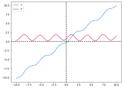
Figure 2: A plot of an arbitrary sinusoidal transformer $\tau$and its first derivative $\tau^{\prime}$. $\tau$ resembles a staircase running along the diagonal with infinitely many inflection points.

Figure † ‣ 2 shows a plot of a sinusoidal transformer $\tau$ with arbitrary parameter values. We can observe that it assumes a “staircase” shape along the diagonal line $y=x$ with an infinite number of inflection points. As noted in Huang et al. (2018); Jaini et al. (2019), these inflection points are actually critical to modelling multi-modal distributions, especially when the modes are well separated. If in Equation 2 we take $p_{\mathbf{x}}$ to be a uniform mixture of well-separated one-dimensional Gaussians and $p_{\mathbf{z}}$ to be a simple one-dimensional standard Gaussian, then the transformation $T^{-1}$ that takes any $x$ into $z$ must

• plateau in regions between any two modes of $p_{\mathbf{x}}$ where there is nearly zero density; and

• admit a sharp jump around a mode of $p_{\mathbf{x}}$.

This can be seen directly from Equation 2. When $p_{\mathbf{x}}\left(x\right)$ is nearly zero, either $p_{\mathbf{z}}\left(T^{-1}\left(x\right)\right)$ or $\lvert\mathrm{det}\,\mathbf{J}_{T^{-1}}\left(x\right)\rvert$ must be close to zero; however, being a standard Gaussian, $p_{\mathbf{z}}$ is near zero only at its boundaries, so for the $99.7\%$ of $x$ that gets mapped to $[-3,3]$, $\lvert\mathrm{det}\,\mathbf{J}_{T^{-1}}\left(x\right)\rvert=\lvert dT^{-1}/dx\rvert$ must be close to zero and hence $T^{-1}$ plateaus. On the other hand, when $p_{\mathbf{x}}$ undergoes a drastic change around a mode, $\lvert dT^{-1}/dx\rvert$ must first explode and then vanish, forcing $T^{-1}$ to make a sharp jump, as $p_{\mathbf{z}}$ is not flexible enough to change so quickly. Therefore, accurately modelling a multi-modal distribution with well-separated modes potentially requires a $T^{-1}$ capable of creating a large number of sharp jumps like a step function.

We claim that our proposed sinusoidal transformer has this inductive bias built in, which makes it suitable for modelling multi-modal distributions. Indeed, as shown in Figure † ‣ 2, it already resembles a step function at initialisation and the distance between any two jumps can be easily adjusted to fit the data by adjusting the periods of the constituent sinusoidals. To further verify our claim, we fit an unconditional Sinusoidal Flow composed of purely “D-scale” transformations to data generated from a uniform mixture of seven one-dimensional Gaussians, and compare the learned density and transformation with that learned by an MAF (Papamakarios et al., 2017). We can see from Figure 3 that our Sinusoidal Flow is not only able to learn the true density well, but can also recover the true transformation $T^{-1}$ which is characterised by “six steps”. Interestingly, the learned transformation only approximates (in fact, only needs to approximate) the true transformation well for $z$ in the interval $[-3,3]$, because outside the interval $p_{\mathbf{z}}$ is nearly zero.

Figure 3: Comparison of Sinusoidal Flow and MAF (Papamakarios et al., 2017) on fitting a multi-modal distribution. Left: density and transformation learned by Sinusoidal Flow. Right: density and transformation learned by MAF. With sinusoidal transformers, Sinusoidal Flow is able to learn the step-function-like true transformation while MAF can only learn an affine transformation.

3.4 Fast Inversion

We now discuss the invertibility of the transformations $L_{l}^{-1}$, $D_{l}^{-1}$ and $U_{l}^{-1}$, as they jointly determine the invertibility of each LDU block. With sinusoidal transformers acting on each input component, we can write $D_{l}^{-1}$ in vector form as

$$\mathbf{z}^{l}=D_{l}^{-1}(\mathbf{z}^{l-1})=\mathbf{z}^{l-1}+G(\mathbf{z}^{l-1})$$ (18)

where $G:\mathbb{R}^{D}\mapsto\mathbb{R}^{D}$ applies the residual function $g$ defined in Equation 15 to each component of the input $\mathbf{z}^{l-1}$. We have shown that the scalar function $g$ is a contraction mapping under the assumption of an independent conditioner, but not yet that the vector-valued function $G$ is also a contraction mapping, which we now prove.

Proposition 3.1.

The function $G$ defined in Equation 18 is a contraction mapping. Specifically, for any $\mathbf{u},\mathbf{v}\in\mathbb{R}^{D}$, $\left\lVert G\left(\mathbf{u}\right)-G\left(\mathbf{v}\right)\right\rVert\leq M\left\lVert\mathbf{u}-\mathbf{v}\right\rVert$ for some $0\leq M<1$.

Proof 3.2.

It is sufficient to prove the proposition with respect to the $\ell_{1}$ norm, since all norms are equivalent in $\mathbb{R}^{D}$.

We have $\left\lVert G\left(\mathbf{u}\right)-G\left(\mathbf{v}\right)\right\rVert=\sum_{i}\lvert g\left(u_{i}\right)-g\left(v_{i}\right)\rvert$ and $\left\lVert\mathbf{u}-\mathbf{v}\right\rVert=\sum_{i}\lvert u_{i}-v_{i}\rvert$ by definition. Because $g$ is a contraction mapping, there exists an $0\leq M_{i}<1$ for each $i$ such that $\lvert g\left(u_{i}\right)-g\left(v_{i}\right)\rvert\leq M_{i}\lvert u_{i}-v_{i}\rvert$. Let $0\leq M=\max_{i}M_{i}<1$, then we must have

$$\sum_{i}\lvert g\left(u_{i}\right)-g\left(v_{i}\right)\rvert\leq\sum_{i}M_{i}\lvert u_{i}-v_{i}\rvert\leq M\sum_{i}\lvert u_{i}-v_{i}\rvert$$

which is the same as $\left\lVert G\left(\mathbf{u}\right)-G\left(\mathbf{v}\right)\right\rVert\leq M\left\lVert\mathbf{u}-\mathbf{v}\right\rVert$.

Algorithm 1 Inversion of $D_{l}^{-1}$

  Input: output $\mathbf{z}^{l}$ from $D_{l}^{-1}$; max number of iterations $n$; error tolerance $\epsilon$

  Initialise $\mathbf{z}^{l}_{0}\vcentcolon=\mathbf{z}^{l}$, $j\vcentcolon=-1$.

  repeat

     $j\vcentcolon=j+1$

     $\mathbf{z}^{l}_{j+1}\vcentcolon=\mathbf{z}^{l}-(D_{l}^{-1}(\mathbf{z}^{l}_{j})-\mathbf{z}^{l}_{j})$

  until $\lVert\mathbf{z}^{l}_{j+1}-\mathbf{z}^{l}_{j}\rVert<\epsilon$ or $j==n$

  return $\mathbf{z}^{l}_{j}$

Proposition 3.1 formally establishes that $D_{l}^{-1}$ is a contractive residual transformation as described in Section 2.2, and as a result, $D_{l}^{-1}$ is fast invertible via Algorithm 1 adapted from Behrmann et al. (2019). In addition, the Banach fixed-point theorem guarantees Algorithm 1 converges with any starting points $\mathbf{z}_{0}^{l}$ at a rate exponential in the number of iterations (Behrmann et al., 2019).

It may be attempting to draw the same conclusion for $L_{l}^{-1}$ and $U_{l}^{-1}$ since they both employ a similar residual structure, but there are no strong theoretical guarantees for them because their conditioners produce input-dependent shifts that dynamically determine the actual transformations. While we could have used spectral normalisation (Miyato et al., 2018) to regularise their conditioners, we observe in practice that Algorithm 1 is still applicable if we use a large number of LDU blocks to share the overall complexity, which is possible only because each LDU block has a built-in residual connection. In the (unlikely) worst case, Algorithm 1 would just resort to a fully vectorised sequential inversion.

Leveraging LDU blocks to introduce full autoregressiveness, we manage to guarantee the core “D-scale” transformations are fast invertible, while the auxiliary shift transformations remain empirically fast invertible. As a result, our Sinusoidal Flow is among the few fully autoregressive flows known to be fast invertible. Song et al. (2019) proposes a Newton-like fixed-point iteration to invert fully autoregressive flows, but their algorithm is only locally convergent and sensitive to starting points; RQ-NSF (Durkan et al., 2019) offers an analytic inverse but their fully autoregressive variant still requires a sequential inversion.

4 Experiments

In this section, we evaluate our Sinusoidal Flow against some common benchmarks to further assess its expressiveness and fast inversion.

4.1 Toy Datasets

Following Wehenkel and Louppe (2019), we first apply our Sinusoidal Flow to a set of toy density estimation problems proposed by Grathwohl et al. (2019). As shown in Figure 4, our Sinusoidal Flow is not only able to capture multi-modal or even discontinuous distributions well, but can also be reliably inverted to generate realistic-looking samples from the learned distributions using Algorithm 1, which further corroborates our claim in Section 3.3 that the inductive bias built into our sinusoidal transformers, which favours step-function-like transformations, enables Sinusoidal Flow to accurately model multi-modal distributions.

Figure 4: A Sinusoidal Flow composed of 16 LDU blocks fit to a set of toy density estimation problems proposed by Grathwohl et al. (2019). Top row: the true distributions. Middle row: the learned distributions. Bottom row: samples generated from the learned distributions.

Table 3: Average negative test log-likelihood in nats over five runs (except for RQ-NSF) on the five real-world datasets from Papamakarios et al. (2017). Lower is better.

Method	POWER	GAS	HEPMASS	MINIBOONE	BSDS300
FFJORD (Grathwohl et al., 2019)	-0.46 $\pm$ 0.01	-8.59 $\pm$ 0.12	14.92 $\pm$ 0.08	10.43 $\pm$ 0.04	-157.40 $\pm$ 0.19
RealNVP (Dinh et al., 2017)	-0.17 $\pm$ 0.01	-8.33 $\pm$ 0.14	18.71 $\pm$ 0.02	13.55 $\pm$ 0.49	-153.28 $\pm$ 1.78
Glow (Kingma and Dhariwal, 2018)	-0.17 $\pm$ 0.01	-8.15 $\pm$ 0.40	19.92 $\pm$ 0.08	11.35 $\pm$ 0.07	-155.07 $\pm$ 0.03
RQ-NSF(C) (Durkan et al., 2019)	-0.64 $\pm$ 0.01	-13.09 $\pm$ 0.02	14.75 $\pm$ 0.03	9.67 $\pm$ 0.47	-157.54 $\pm$ 0.28
MAF (Papamakarios et al., 2017)	-0.24 $\pm$ 0.01	-10.08 $\pm$ 0.02	17.70 $\pm$ 0.02	11.75 $\pm$ 0.44	-155.69 $\pm$ 0.28
TAN (Oliva et al., 2018)	-0.60 $\pm$ 0.01	-12.06 $\pm$ 0.02	13.78 $\pm$ 0.02	11.01 $\pm$ 0.48	-159.80 $\pm$ 0.07
NAF (Huang et al., 2018)	-0.62 $\pm$ 0.01	-11.96 $\pm$ 0.33	15.09 $\pm$ 0.40	8.86 $\pm$ 0.15	-157.73 $\pm$ 0.30
B-NAF (De Cao et al., 2020)	-0.61 $\pm$ 0.01	-12.06 $\pm$ 0.09	14.71 $\pm$ 0.38	8.95 $\pm$ 0.07	-157.36 $\pm$ 0.03
SOS (Jaini et al., 2019)	-0.60 $\pm$ 0.01	-11.99 $\pm$ 0.41	15.15 $\pm$ 0.10	8.90 $\pm$ 0.11	-157.48 $\pm$ 0.41
UMNN-MAF (Wehenkel and Louppe, 2019)	-0.63 $\pm$ 0.01	-10.89 $\pm$ 0.70	13.99 $\pm$ 0.21	9.67 $\pm$ 0.13	-157.98 $\pm$ 0.01
RQ-NSF(AR) (Durkan et al., 2019)	-0.66 $\pm$ 0.01	-13.09 $\pm$ 0.02	14.01 $\pm$ 0.03	9.22 $\pm$ 0.48	-157.31 $\pm$ 0.28
Sinusoidal Flow (Ours)	-0.59 $\pm$ 0.00	-12.15 $\pm$ 0.05	16.10 $\pm$ 0.06	9.25 $\pm$ 0.03	-156.75 $\pm$ 0.03

4.2 Real-world Datasets

We compare our Sinusoidal Flow with several other normalising flows on five high-dimensional real-world datasets (POWER, GAS, HEPMASS, MINIBOONE and BSDS300) proposed by Papamakarios et al. (2017). From Table 3 we observe that, while no method can claim the best performance across all five datasets, Sinusoidal Flow is comparable to those top-performing methods on each dataset, with an (additional) advantage of being fast invertible.

Table 4: Bits/dim on MNIST and CIFAR-10. Lower is better.

Method	MNIST	CIFAR-10
FFJORD (Grathwohl et al., 2019)	0.99	3.40
i-ResNet (Behrmann et al., 2019)	1.06	3.45
RealNVP (Dinh et al., 2017)	1.06	3.49
Glow (Kingma and Dhariwal, 2018)	1.05	3.35
RQ-NSF(C) (Durkan et al., 2019)	-	3.38
MAF (Papamakarios et al., 2017)	1.89	4.31
TAN (Oliva et al., 2018)	1.19	3.98
SOS (Jaini et al., 2019)	1.81	-
UMNN-MAF (Wehenkel and Louppe, 2019)	1.13	-
Sinusoidal Flow (Ours)	1.06	3.51

To further assess its efficacy in modelling high-dimensional data like images, we apply our Sinusoidal Flow to MNIST (Lecun et al., 1998) and CIFAR-10 (Krizhevsky, 2009) pre-processed by Papamakarios et al. (2017). Unlike existing work that uses a carefully engineered multi-scale convolutional architecture (Dinh et al., 2017), we simply adopt a miniature PixelCNN (van den Oord et al., 2016) as the conditioners for the shift transformations in each LDU block. As shown in Table 4, compared to other fully autoregressive flows that ever managed to model images without an explosion in parameters, our Sinusoidal Flow achieves results much closer to that achieved by methods with convolutional architectures. Moreover, in Figure 5 we can see some reasonable runtimes for both generating and reconstructing CIFAR-10 images at different tolerance levels and maximum iterations allowed at each LDU block, which reaffirms that our Sinusoidal Flow is fast invertible.

Figure 5: Left: Runtimes for generation. Right: Runtimes for reconstruction. rtol and atol refer to the corresponding arguments of a typical allclose function.

5 Conclusions

We recognise expressiveness, fast inversion and exact Jacobian determinant as three properties desirable for normalising flows. Leveraging the fact that the integral of a sinusoidal function squared resembles a residual transformation, Sinusoidal Flow represents an interesting attempt at integrating the respective strengths of fully autoregressive flows and contractive residual flows in order to excel at all three dimensions. Our unique design of the LDU blocks offers a new way of introducing full autoregressiveness without hurting the invertibility of the core transformations and naturally ensures an easy Jacobian determinant.

References

- Bachlechner et al. (2020) Thomas Bachlechner, Bodhisattwa Prasad Majumder, Huanru Henry Mao, Garrison W. Cottrell, and Julian McAuley. Rezero is all you need: Fast convergence at large depth, 2020.
- Behrmann et al. (2019) Jens Behrmann, Will Grathwohl, Ricky T. Q. Chen, David Duvenaud, and Joern-Henrik Jacobsen. Invertible residual networks. In Kamalika Chaudhuri and Ruslan Salakhutdinov, editors, Proceedings of the 36th International Conference on Machine Learning, volume 97 of Proceedings of Machine Learning Research, pages 573–582. PMLR, 09–15 Jun 2019.
- Casella and Berger (2001) George Casella and Roger Berger. Statistical Inference. Duxbury Resource Center, June 2001. ISBN 0534243126.
- Chen et al. (2018) Ricky T. Q. Chen, Yulia Rubanova, Jesse Bettencourt, and David K Duvenaud. Neural ordinary differential equations. In S. Bengio, H. Wallach, H. Larochelle, K. Grauman, N. Cesa-Bianchi, and R. Garnett, editors, Advances in Neural Information Processing Systems, volume 31, pages 6571–6583. Curran Associates, Inc., 2018.
- De Cao et al. (2020) Nicola De Cao, Wilker Aziz, and Ivan Titov. Block neural autoregressive flow. In Ryan P. Adams and Vibhav Gogate, editors, Proceedings of The 35th Uncertainty in Artificial Intelligence Conference, volume 115 of Proceedings of Machine Learning Research, pages 1263–1273, Tel Aviv, Israel, 22–25 Jul 2020. PMLR.
- Dinh et al. (2015) Laurent Dinh, David Krueger, and Yoshua Bengio. Nice: Non-linear independent components estimation, 2015.
- Dinh et al. (2017) Laurent Dinh, Jascha Sohl-Dickstein, and Samy Bengio. Density estimation using real NVP. In 5th International Conference on Learning Representations, ICLR 2017, Toulon, France, April 24-26, 2017, Conference Track Proceedings. OpenReview.net, 2017.
- Durkan et al. (2019) Conor Durkan, Artur Bekasov, Iain Murray, and George Papamakarios. Neural spline flows. In H. Wallach, H. Larochelle, A. Beygelzimer, F. d'Alché-Buc, E. Fox, and R. Garnett, editors, Advances in Neural Information Processing Systems, volume 32. Curran Associates, Inc., 2019.
- Germain et al. (2015) Mathieu Germain, Karol Gregor, Iain Murray, and Hugo Larochelle. Made: Masked autoencoder for distribution estimation. In Francis Bach and David Blei, editors, Proceedings of the 32nd International Conference on Machine Learning, volume 37 of Proceedings of Machine Learning Research, pages 881–889, Lille, France, 07–09 Jul 2015. PMLR.
- Grathwohl et al. (2019) Will Grathwohl, Ricky T. Q. Chen, Jesse Bettencourt, and David Duvenaud. Scalable reversible generative models with free-form continuous dynamics. In International Conference on Learning Representations, 2019.
- He et al. (2016) K. He, X. Zhang, S. Ren, and J. Sun. Deep residual learning for image recognition. In 2016 IEEE Conference on Computer Vision and Pattern Recognition (CVPR), pages 770–778, 2016. 10.1109/CVPR.2016.90.
- Ho et al. (2019) Jonathan Ho, Xi Chen, Aravind Srinivas, Yan Duan, and Pieter Abbeel. Flow++: Improving flow-based generative models with variational dequantization and architecture design. In Kamalika Chaudhuri and Ruslan Salakhutdinov, editors, Proceedings of the 36th International Conference on Machine Learning, volume 97 of Proceedings of Machine Learning Research, pages 2722–2730. PMLR, 09–15 Jun 2019.
- Huang et al. (2018) Chin-Wei Huang, David Krueger, Alexandre Lacoste, and Aaron Courville. Neural autoregressive flows. In Jennifer Dy and Andreas Krause, editors, Proceedings of the 35th International Conference on Machine Learning, volume 80 of Proceedings of Machine Learning Research, pages 2078–2087, StockholmsmÀssan, Stockholm Sweden, 10–15 Jul 2018. PMLR.
- Jaini et al. (2019) Priyank Jaini, Kira A. Selby, and Yaoliang Yu. Sum-of-squares polynomial flow. In Kamalika Chaudhuri and Ruslan Salakhutdinov, editors, Proceedings of the 36th International Conference on Machine Learning, volume 97 of Proceedings of Machine Learning Research, pages 3009–3018. PMLR, 09–15 Jun 2019.
- Kingma and Dhariwal (2018) Durk P Kingma and Prafulla Dhariwal. Glow: Generative flow with invertible 1x1 convolutions. In S. Bengio, H. Wallach, H. Larochelle, K. Grauman, N. Cesa-Bianchi, and R. Garnett, editors, Advances in Neural Information Processing Systems, volume 31, pages 10215–10224. Curran Associates, Inc., 2018.
- Kingma et al. (2016) Durk P Kingma, Tim Salimans, Rafal Jozefowicz, Xi Chen, Ilya Sutskever, and Max Welling. Improved variational inference with inverse autoregressive flow. In D. Lee, M. Sugiyama, U. Luxburg, I. Guyon, and R. Garnett, editors, Advances in Neural Information Processing Systems, volume 29, pages 4743–4751. Curran Associates, Inc., 2016.
- Krizhevsky (2009) Alex Krizhevsky. Learning multiple layers of features from tiny images. Technical report, 2009.
- Lecun et al. (1998) Y. Lecun, L. Bottou, Y. Bengio, and P. Haffner. Gradient-based learning applied to document recognition. Proceedings of the IEEE, 86(11):2278–2324, 1998.
- Ma et al. (2019) Xuezhe Ma, Xiang Kong, Shanghang Zhang, and Eduard Hovy. Macow: Masked convolutional generative flow. In H. Wallach, H. Larochelle, A. Beygelzimer, F. d'Alché-Buc, E. Fox, and R. Garnett, editors, Advances in Neural Information Processing Systems, volume 32, pages 5893–5902. Curran Associates, Inc., 2019.
- Miyato et al. (2018) Takeru Miyato, Toshiki Kataoka, Masanori Koyama, and Yuichi Yoshida. Spectral normalization for generative adversarial networks. In International Conference on Learning Representations, 2018.
- Müller et al. (2019) Thomas Müller, Brian Mcwilliams, Fabrice Rousselle, Markus Gross, and Jan Novák. Neural importance sampling. ACM Trans. Graph., 38(5), October 2019. ISSN 0730-0301.
- Oliva et al. (2018) Junier Oliva, Avinava Dubey, Manzil Zaheer, Barnabas Poczos, Ruslan Salakhutdinov, Eric Xing, and Jeff Schneider. Transformation autoregressive networks. In Jennifer Dy and Andreas Krause, editors, Proceedings of the 35th International Conference on Machine Learning, volume 80 of Proceedings of Machine Learning Research, pages 3898–3907, StockholmsmÀssan, Stockholm Sweden, 10–15 Jul 2018. PMLR.
- Papamakarios et al. (2017) George Papamakarios, Theo Pavlakou, and Iain Murray. Masked autoregressive flow for density estimation. In I. Guyon, U. V. Luxburg, S. Bengio, H. Wallach, R. Fergus, S. Vishwanathan, and R. Garnett, editors, Advances in Neural Information Processing Systems, volume 30, pages 2338–2347. Curran Associates, Inc., 2017.
- Papamakarios et al. (2019) George Papamakarios, Eric Nalisnick, Danilo Jimenez Rezende, Shakir Mohamed, and Balaji Lakshminarayanan. Normalizing flows for probabilistic modeling and inference, 2019.
- Rezende and Mohamed (2015) Danilo Rezende and Shakir Mohamed. Variational inference with normalizing flows. In Francis Bach and David Blei, editors, Proceedings of the 32nd International Conference on Machine Learning, volume 37 of Proceedings of Machine Learning Research, pages 1530–1538, Lille, France, 07–09 Jul 2015. PMLR.
- Song et al. (2019) Yang Song, Chenlin Meng, and Stefano Ermon. Mintnet: Building invertible neural networks with masked convolutions. In H. Wallach, H. Larochelle, A. Beygelzimer, F. d'Alché-Buc, E. Fox, and R. Garnett, editors, Advances in Neural Information Processing Systems, volume 32, pages 11004–11014. Curran Associates, Inc., 2019.
- Tabak and Turner (2013) E. G. Tabak and Cristina V. Turner. A family of nonparametric density estimation algorithms. Communications on Pure and Applied Mathematics, 66(2):145–164, 2013.
- van den Berg et al. (2019) Rianne van den Berg, Leonard Hasenclever, Jakub M. Tomczak, and Max Welling. Sylvester normalizing flows for variational inference, 2019.
- van den Oord et al. (2016) Aaron van den Oord, Nal Kalchbrenner, Lasse Espeholt, koray kavukcuoglu, Oriol Vinyals, and Alex Graves. Conditional image generation with pixelcnn decoders. In D. Lee, M. Sugiyama, U. Luxburg, I. Guyon, and R. Garnett, editors, Advances in Neural Information Processing Systems, volume 29. Curran Associates, Inc., 2016.
- Wehenkel and Louppe (2019) Antoine Wehenkel and Gilles Louppe. Unconstrained monotonic neural networks. In H. Wallach, H. Larochelle, A. Beygelzimer, F. d'Alché-Buc, E. Fox, and R. Garnett, editors, Advances in Neural Information Processing Systems, volume 32, pages 1545–1555. Curran Associates, Inc., 2019.