Robust Ellipsoid-specific Fitting via Expectation Maximization

Abstract

Ellipsoid fitting is of general interest in machine vision, such as object detection and shape approximation. Most existing approaches rely on the least-squares fitting of quadrics, minimizing the algebraic or geometric distances, with additional constraints to enforce the quadric as an ellipsoid. However, they are susceptible to outliers and non-ellipsoid or biased results when the axis ratio exceeds certain thresholds.

To address these problems, we propose a novel and robust method for ellipsoid fitting in a noisy, outlier-contaminated 3D environment. We explicitly model the ellipsoid by kernel density estimation (KDE) of the input data. The ellipsoid fitting is cast as a maximum likelihood estimation (MLE) problem without extra constraints, where a weighting term is added to depress outliers, and then effectively solved via the Expectation-Maximization (EM) framework. Furthermore, we introduce the vector $\varepsilon$ technique to accelerate the convergence of the original EM. The proposed method is compared with representative state-of-the-art approaches by extensive experiments, and results show that our method is ellipsoid-specific, parameter free, and more robust against noise, outliers, and the large axis ratio. Our implementation is available at https://zikai1.github.io/.

1 Introduction

Detecting and fitting quadratic surfaces or quadrics from 3D scattered points, such as planes, cylinders, and ellipsoids is a fundamental problem in machine vision [Miller(1988), Faber and Fisher(2001), Bischoff and Kobbelt(2002), Blane et al.(2000)Blane, Lei, Civi, and Cooper, Allaire et al.(2007)Allaire, Jacq, Burdin, Roux, and Couture, Georgiev et al.(2016)Georgiev, Al-Hami, and Lakaemper, Beale et al.(2016)Beale, Yang, Campbell, Cosker, and Hall]. Among quadrics, ellipsoids attract more interest because they are the uniquely bounded and centric surface, which provides a good characterization or approximation for the center and orientation of objects [Tasdizen(2001), Li and Griffiths(2004), Nikolaos Kyriazis and Argyros(2011)]. For instance, Rimon et al [Rimon and Boyd(1997)] use ellipsoid fitting to approximate the robot shape and speed up the collision detection process. Jia et al [Jia et al.(2011)Jia, Choi, Mourrain, and Wang] take ellipsoids as bounding box for continuous collision detection. Gietzelt et al[Gietzelt et al.(2013)Gietzelt, Wolf, Marschollek, and Haux] reduce the accelerometer calibration as a 3D ellipsoid fitting problem, by which the transformation and correction matrix is identified.

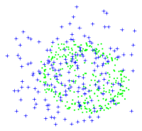
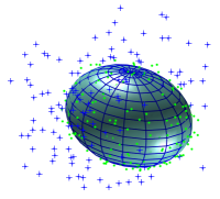
(a) Outlier-contaminated fitting

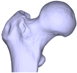
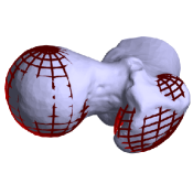
(b) 3D medical data

Figure 1: Our method shows (a) highly accurate fitting in the contamination of heavy outliers (‘+’) (net ellipsoid is the ground truth), and (b) approximation for 3D medical femur images.

Most existing methods adopt the least-squares (LS) principle for ellipsoid fitting, among which algebraic or geometric distances are minimized. These methods attain satisfactory results for simple and low-noise data points but are susceptible to outliers that are quite common and inevitable in practice [Birdal et al.(2019)Birdal, Busam, Navab, Ilic, and Sturm, Thurnhofer-Hemsi et al.(2020)Thurnhofer-Hemsi, López-Rubio, Blázquez-Parra, Ladrón-de Guevara-Muñoz, and de Cózar-Macias, Zhao et al.(2021)Zhao, Jia, Fan, Liang, and Yan]. Meanwhile, various constraints have been investigated to force the fitted surface as an ellipsoid regardless of the input data. However, they cannot guarantee the best fitting when the ratio between the longest axis and the shortest one surpasses certain thresholds, such as two in [Li and Griffiths(2004)] and [Kesäniemi and Virtanen(2017)], thereby significantly limiting their applications.

To overcome the shortcomings above, we propose a novel ellipsoid fitting method that dose not relying on LS, instead, by using a set of points sampled over a unit sphere and transformed by the model parameters, which is highly robust against outliers, and is ellipsoid-specific regardless of the axis ratio. Inspired by a study of the point set registration framework in [Myronenko and Song(2010)], we explicitly model the ellipsoid and represent it via Gaussian mixture models (GMM), armed with an adaptive uniform distribution to depress outliers. Then ellipsoid fitting is formulated as an MLE without extra constraints, which is effectively solved by the expectation-maximization (EM) framework. Furthermore, we encapsulate all parameters into a sequence and introduce the vector $\varepsilon$ algorithm [Wang et al.(2008)Wang, Kuroda, Sakakihara, and Geng] to accelerate the EM convergence.

Our method is robust enough against outliers up to 60% and is without handcraft tuning of hyper-parameters. The performance of our method regarding the accuracy and robustness is validated by measuring the offset and shape deviations on various numerical experiments. We further demonstrate the promising applications of the proposed method on real-world scanned point clouds, where occlusion and outliers exist. Furthermore, our method can be directly generalized to fit other quadrics such as cylinders and cones, as long as a parametric representation is given. To summarize, the contributions of this work are threefold as follows:

• A novel ellipsoid-specific fitting method with remarkable robustness against outliers, noise and the axis ratio.

• The probabilistic method is applied for ellipsoid fitting. We explicitly model the ellipsoid based on the outlier analysis from the kernel density estimation and effectively speed up the convergence of the EM framework.

• All parameters are updated automatically by the derivation of the analytical gradients without user tuning.

2 Related Work

Definition 1

A general quadric in 3D Euclidean space is defined by the zero set of a second order polynomial:

$$\begin{aligned} Q(\mathbf{a},\mathbf{p})=\mathbf{a}\cdot\mathbf{p}&=Ax^{2}+By^{2}+Cz^{2}+2Dxy+2Exz\\ &+2Fyz+2Gx+2Hy+2Iz+J=0,\end{aligned}$$ (1)

where $\mathbf{a}=[x^{2}\quad y^{2}\quad z^{2}\quad 2xy\quad 2xz\quad 2yz\quad 2x\quad 2y\quad 2z\quad 1]^{T}$ are built from the point $\mathbf{x}=(x,y,z)^{T}\in\mathbb{R}^{3}$, and $\mathbf{p}=[A\quad B\quad C\quad D\quad E\quad F\quad G\quad H\quad I\quad J]^{T}$ are the coefficients that characterize the quadric.

Eq. 1 represents an ellipsoid if its quadratic invariants satisfy [Harris and Stöcker(1998)]

$$I_{1}>0,\quad I_{2}*I_{3}>0,$$ (2)

where $I_{1}=AB+AC+BC-D^{2}-E^{2}-F^{2}$, $I_{2}=A+B+C$, and

$$I_{3}=\left|\begin{array}[]{ccc}A&D&E\\ D&B&F\\ F&E&C\\ \end{array}\right|.$$ (6)

Given a set of data points $\mathbf{X}=\{\mathbf{x}_{i}\in\mathbb{R}^{3}\}_{i=1}^{N}$ that are sampled from a potential ellipsoid possibly with noise or outliers, our purpose is to fit an ellipsoid from the data. The most frequently used methods are those based on the LS principle, which can be classified into algebraic and geometric fittings.

Algebraic fitting. To find the optimal parameter $\mathbf{p}$, algebraic fitting minimizes the deviation of the polynomial in Eq. 1 (ie, the algebraic distance or equation error) [Fitzgibbon and Fisher(1995)] by

$$\sum_{i=1}^{N}Q^{2}(\mathbf{a}_{i},\mathbf{p})=\sum_{i=1}^{N}(\mathbf{p}^{T}\mathbf{a}_{i})^{2}=\mathbf{p}^{T}\mathbf{Q}\mathbf{p},$$ (7)

where $\mathbf{a}_{i}=\mathbf{a}(\mathbf{x}_{i})$ is the vector corresponding to the $i^{th}$ point $\mathbf{x}_{i}=(x_{i},y_{i},z_{i})^{T}$, and $\mathbf{Q}=\sum_{i=1}^{N}\mathbf{a}_{i}\mathbf{a}_{i}^{T}\in\mathbb{S}^{10}$ is the scatter matrix. Ellipse-specific fitting in 2D is solved by Fitzgibbon et al [Fitzgibbon et al.(1999)Fitzgibbon, Pilu, and Fisher], and a direct extension for 3D ellipsoid-specific case is presented in [Li and Griffiths(2004)] under the determinant $(A-B-C)^{2}-4(F^{2}+G^{2}+H^{2}+BC)>0.$ Nevertheless, it attains a best fit only when the shortest axis of the ellipsoid is at least half of the longest one. Once this hypothesis fails, a bisection search must be executed to provide an approximation. Thus it may deviate from the ground truths. Recently, Kesäniemi et al [Kesäniemi and Virtanen(2017)] elaborate previous approaches and simultaneously consider three trace constraints $D^{2}-AB<0,E^{2}-AC<0,$ and $F^{2}-BC<0$, to force the quadric to be an ellipsoid, but it only credibly fits ellipsoids with a prior that their maximal axis ratio $r_{ax}<\sqrt{\frac{2d-2}{d-2}}$, where $d$ is the dimension. When $d=3$ in our case, the limit value $r_{ax}=2$, meaning that it may fail to fit an ellipsoid whose longest axis is more than twice the shortest one. Therefore, similar to [Li and Griffiths(2004)], the application scope of [Kesäniemi and Virtanen(2017)] is also greatly confined. Furthermore, according to the Gauss-Markov theorem [Rousseeuw and Leroy(2005)], LS fitting is susceptible to outliers that are quite common in practice.

Several methods [Calafiore(2002), Ying et al.(2012)Ying, Yang, and Zha] treat ellipsoid fitting as a semi-definite programming (SDP) problem, where ellipsoid-specificity is formalized as the matrix semi-definiteness such that $S_{p}(\mathbf{A})\succeq 0$, where $S_{p}(\cdot)$ is the operator that extracts the leading $p\times p$ principal submatrix of $\mathbf{A}$. Lin et al [Lin and Huang(2015)] introduce alternating direction method of multipliers (ADMM) to speed up SDP solving but still minimize the residual error $\|\mathbf{a}_{i}^{T}\mathbf{p}\|_{2}$ in the LS sense, thereby their method is sensitive to outlier-contaminated environment.

Geometric fitting. Alternatively, geometric fitting [Gander et al.(1994)Gander, Golub, and Strebel, Ahn et al.(2002)Ahn, Rauh, Cho, and Warnecke] minimizes the orthogonal distance from point $\mathbf{x}_{i},i=1,\cdots,N$, to the ellipsoid

$${\mathop{\mathrm{dist}}}(\mathbf{X},Q)=\sum_{i=1}^{N}\|\mathbf{x}_{i}-\bar{\mathbf{x}}_{i}\|^{2}=\sum_{i=1}^{N}d_{i}^{2},$$ (8)

where $\bar{\mathbf{x}}_{i}$ is the point on the ellipsoid closet to $\mathbf{x}_{i}$, and $\|\mathbf{x}-\bar{\mathbf{x}}_{i}\|$ denotes the Euclidean distance between $\mathbf{x}$ and $\mathbf{x}_{i}$. Geometric fitting exhibits more sound physical interpretations and higher accuracy than algebraic fitting, but it requires much more time for distance evaluation. Calculating the exact Euclidean distance from a point to an ellipsoid requires solving a sixth-order equation. We present a simple derivation on the exact computation in the supplemental material. To circumvent this issue, Taubin [Taubin(1991)] uses the second-order Taylor expansion to approximate the orthogonal distance, whereas Sampson [Sampson(1982)] weights the algebraic distance by the first-order differential. However, geometric fitting usually requires proper initialization (from algebraic fitting), and it is also vulnerable to outliers because the objective function (Eq. 8) is based on the LS principle. Later, iteratively re-weighted least-squares (IRLS) is introduced to depress outliers, by which M-estimators (robust kernels), such as Tukey [Rousseeuw(1991)] and Huber [Huber(2004)], are used to reduce the effect of large residuals. IRLS is more stable and robust than ordinary least-squares in an outlier-contaminated environment.

3 Methodology

Analysis of the input data. For the given data points $\mathbf{X}=\{\mathbf{x}_{i}\in\mathbb{R}^{3}\}_{i=1}^{N}$, suppose $\mathbf{X}\sim p(\mathbf{x})$, ie, $\mathbf{X}$ satisfies the probability distribution $p(\mathbf{x})$, then we use the KDE to model the point density by $p(\mathbf{x})=\frac{1}{N}\sum_{i=1}^{N}K_{h}(\mathbf{x}-\mathbf{x}_{i}),$ where $K_{h}(\mathbf{x}-\mathbf{x}_{i})$ is the kernel function, and $h$ is the kernel bandwidth. A universal kernel is Gaussian function, which gives rise to the following Gaussian mixture model:

$$p(\mathbf{x})=\frac{1}{N}\sum_{i=1}^{N}\frac{1}{(2\pi h^{2})^{d/2}}\exp(-\frac{\|\mathbf{x}-\mathbf{x}_{i}\|^{2}}{2h^{2}}),$$ (9)

where $d$ denotes the dimension ($d=3$ in our case). Despite that Gaussian kernel function is broadly used, the choice of a globally suitable $h$ is not easy [Bishop(2006)]. To ease this problem, from the theory in [Tang and He(2017)] we adopt the local region for density estimation.

The $k$-nearest neighbour of $\mathbf{x}_{i},i=1,\cdots,N$, is denoted as $\textrm{N}(\mathbf{x}_{i})=\{\textrm{N}_{1}(\mathbf{x}_{i}),\textrm{N}_{2}(\mathbf{x}_{i}),\cdots,\textrm{N}_{k}(\mathbf{x}_{i})\}.$ Then the density at $\mathbf{x}_{i}$ is calculated by $p(\mathbf{x}_{i})=\frac{1}{k+1}\sum_{\mathbf{x}\in\textrm{N}(\mathbf{x}_{i})\cup\{\mathbf{x}_{i}\}}\frac{1}{(2\pi h^{2})^{d/2}}\exp(-\frac{\|\mathbf{x}-\mathbf{x}_{i}\|^{2}}{2h^{2}}).$ We leverage kd-tree [Bentley(1975)] to reduce the computational complexity from $O(N^{2})$ to $O(N\log N)$. Different from [Tang and He(2017)] utilizing the same local $h$, we associate location $\mathbf{x}_{i}$ in the data space with kernel bandwidth $h$ by adaptively calculating the local covariance $h=\frac{1}{k}\sum_{\mathbf{x}\in\textrm{N}(\mathbf{x}_{i})}(\mathbf{x}-\mathbf{x}_{i})^{T}(\mathbf{x}-\mathbf{x}_{i}).$

After the density estimation of each point $\mathbf{x}_{i}\in\mathbf{X}$, we adopt the relative density-based outlier score (RDOS) [Tang and He(2017)] to measure the extent of point $\mathbf{x}_{i}$, differing from its neighbourhood $\textrm{N}(\mathbf{x}_{i})$, according to the following ratio

$${\mathop{\mathrm{RDOS}}}(\mathbf{x}_{i})=\frac{\sum_{\mathbf{x}\in\textrm{N}(\mathbf{x}_{i})}p(\mathbf{x})}{|\textrm{N}(\mathbf{x}_{i})|p(\mathbf{x}_{i})}.$$ (10)

Intuitively, a larger ${\mathop{\mathrm{RDOS}}}(\mathbf{x}_{i})$ indicates that $\mathbf{x}_{i}$ is outside a dense region. Thus it is more likely to be an outlier; otherwise, $\mathbf{x}_{i}$ can be deemed as non-outlier. We further use Lemma 1 to attain a quantitative analysis.

Lemma 1

Let the points $\mathbf{X}=\{\mathbf{x}_{i}\in\mathbb{R}^{3}\}_{i=1}^{N}$ be sampled from a continuous density distribution and the kernel function $K_{h}(x)$ be non-negative everywhere and integrated to one. Then, ${\mathop{\mathrm{RDOS}}}(\mathbf{x}_{i})$ equals 1 with probability 1:

$$\lim_{N\longrightarrow\infty}P({\mathop{\mathrm{RDOS}}}(\mathbf{x}_{i})=1)=1.$$ (11)

Lemma 1 provides a lower bound for outlier recognition. When $0<{\mathop{\mathrm{RDOS}}}(\mathbf{x}_{i})<1$ or ${\mathop{\mathrm{RDOS}}}(\mathbf{x}_{i})\approx 1$, we say that $\mathbf{x}_{i}$ is not an outlier, and $\mathbf{x}_{i}$ is possibly an outlier only if ${\mathop{\mathrm{RDOS}}}(\mathbf{x}_{i})\gg 1$. The adaptive ${\mathop{\mathrm{RDOS}}}(\mathbf{x}_{i})$ is introduced for the weight initialization of our method. Meanwhile it can also be used for ellipsoid modeling, as presented in the following.

Ellipsoid modeling. Suppose the given point set $\mathbf{X}=\{\mathbf{x}_{i}\in\mathbb{R}^{3}\}_{i=1}^{N}$ is fitted by an ellipsoid $e$ with the shape parameter $\bm{\theta}=(x_{0},y_{0},z_{0},a,b,c,\alpha,\beta,\gamma)$, where $(x_{0},y_{0},z_{0})$ is the ellipsoid center, $(a,b,c)$ are the three semi-axis lengths, and $(\alpha,\beta,\gamma)$ are the Euler angles along the $x,y,\text{and}~{}z$ axes. To attain the ellipsoid, we first create a unit sphere $s$ containing points $\mathbf{Y}=\{\mathbf{y}_{m}\in\mathbb{R}^{3}\}_{m=1}^{M}$ defined as

$$x_{m}=x_{c}+\cos\theta_{i}\cdot\sin\psi_{j},\quad y_{m}=y_{c}+\cos\theta_{i}\cdot\cos\psi_{j},\quad z_{m}=z_{c}+\sin\theta_{i},$$ (12)

where $\mathbf{c}_{s}=(x_{c},y_{c},z_{c})$ is the spherical center, $\theta\in[0,\pi)$, $\psi\in[0,2\pi)$. To generate spherical points $\mathbf{y}_{m}$, the number of inliers can be counted as $M=\sum_{\mathbf{x}_{i}\in\mathbf{X}}\mathbbm{1}({\mathop{\mathrm{RDOS}}}(\mathbf{x}_{i})\leq 1)$ (Lemma 1), where $\mathbbm{1}$ is the indicator function. We relax the inlier constraint as $M=\sum_{\mathbf{x}_{i}\in\mathbf{X}}\mathbbm{1}({\mathop{\mathrm{RDOS}}}(\mathbf{x}_{i})\leq 2)$, then $\theta_{i}=\frac{\pi i}{[\sqrt{M}]}$ and $\psi_{j}=\frac{2\pi j}{[\sqrt{M}]},i,j=1,\cdots,[\sqrt{M}]$, where $[\cdot]$ is a rounding function.

Then a linear transformation $\mathcal{T}$ transforms the sphere $s$ to the real ellipsoid $e$ by $e=$$\mathcal{T}(s)=\mathbf{A}s+\mathbf{t},$ where $\mathbf{A}$ is the affine transformation matrix, and $\mathbf{t}$ is the translation vector. To solve $\mathbf{A}$ and $\mathbf{t}$, we formulate ellipsoid fitting as a likelihood estimation by first expressing the sphere model as a GMM with $M$ components, $p(\mathbf{z})=\sum_{m=1}^{M}P(\mathbf{y}_{m})p(\mathbf{z}|\mathbf{y}_{m}),\mathbf{z}\in\mathbb{R}^{3},$ where $p(\mathbf{z}|\mathbf{y}_{m})=\frac{1}{(2\pi\sigma^{2})^{d/2}}\exp(-\frac{\|\mathbf{z}-\mathbf{y}_{m}\|^{2}}{2\sigma^{2}})$ is the Gaussian distribution and $P(\mathbf{y}_{m})$ represents the probability selecting the component $\mathbf{y}_{m}$. To depress outliers, we add an additional uniform distribution $p(\mathbf{z}|\mathbf{y}_{M+1})=\frac{1}{V}$ relative to the volume $V$ of the bounding box of $\mathbf{X}$: $p(\mathbf{z})=w\frac{1}{V}+(1-w)\sum_{m=1}^{M}P(\mathbf{y}_{m})p(\mathbf{z}|\mathbf{y}_{m})$, where $w\in[0,1]$ is the weight to balance the two distributions.

Given that the spherical points $\mathbf{Y}=\{\mathbf{y}_{m}\in\mathbb{R}^{3}\}_{m=1}^{M}$ are generated uniformly, we set equal membership probability $P(\mathbf{y}_{m})=\frac{1}{M}$ and isotropic covariance $\sigma^{2}$ for all components

$$\begin{aligned} p(\mathbf{z})\!=\!\frac{w}{V}\!+\!\frac{1\!-\!w}{M}\sum_{m=1}^{M}(2\pi\sigma^{2})^{-d/2}\exp(-\frac{1}{2\sigma^{2}}\|\mathbf{z}\!-\!\mathbf{y}_{m}\|^{2}).\end{aligned}$$ (13)

The likelihood function $F(\Omega)=\prod_{i=1}^{N}p(\mathbf{x}_{i}|\Omega)$ of the input data $\mathbf{X}=\{\mathbf{x}_{i}\in\mathbb{R}^{3}\}_{i=1}^{N}$ is maximized based on the independent and identical distribution assumption, where $\Omega=\{\mathbf{A},\mathbf{t},\sigma^{2},w\}$ is the parameter set. In [Myronenko and Song(2010)], the weight $w$ is preset as a hyper-parameter and tuned by users. However, we make no assumptions on the noise or outlier magnitude. We take $w$ as a variable and automatically update it to find the optimal value. Finally, maximizing $F(\Omega)$ is equivalent to minimizing the following negative log-posterior

$$\begin{aligned} &E(\Omega|\mathbf{X})=-\sum_{i=1}^{N}\log p(\mathbf{x}_{i}|\Omega)=-\sum_{i=1}^{N}\log(\sum_{m=1}^{M}\frac{1-w}{M}\frac{1}{(2\pi\sigma^{2})^{d/2}}\exp({\frac{\|\mathbf{x}_{i}-(\mathbf{A}\mathbf{y}_{m}+\mathbf{t})\|^{2}}{2\sigma^{2}}})+\frac{w}{V}).\end{aligned}$$ (14)

4 EM Algorithm

We adopt the EM framework [Moon(1996)] for ellipsoid fitting. The basic idea behind is first guessing an "old" parameter $\Omega^{old}$ and then use the Bayesian theorem [Joyce(2003)] to compute a posterior probability or responsibility of the mixture components, which is the expectation or E-step of the algorithm. In the subsequent maximization or M-step, the "new" parameter $\Omega$ is updated by minimizing the expectation of the completed-data negative log-likelihood $Q$ function (detailed in the supplemental material). The update of EM is detailed as follows.

E-step: We compute the posterior probability regarding the uniform distribution and each mixture component in GMM, respectively.

$$\begin{aligned} &p^{old}({\color[rgb]{0,0,0}{\mathbf{y}_{M+1}}}|\mathbf{x}_{i},\Omega)=\frac{\frac{w}{V}}{w\frac{1}{V}+(1-w)\sum_{k=1}^{M}\frac{1}{M}p(\mathbf{x}_{i}|\mathbf{y}_{k})}&p^{old}(\mathbf{y}_{m}|\mathbf{x}_{i},\Omega)=\frac{\frac{1-w}{M}\frac{1}{(2\pi\sigma^{2})^{d/2}}\exp({\frac{-\|\mathbf{x}_{i}-\mathbf{A}^{old}\mathbf{y}_{m}+\mathbf{t}^{old})\|^{2}}{2\sigma^{2}}})}{w\frac{1}{V}+(1-w)\sum_{k=1}^{M}\frac{1}{M}p(\mathbf{x}_{i}|\mathbf{y}_{k})}\\ &=\frac{1}{1+\frac{V}{M}\frac{1-w}{w}\sum_{k=1}^{m}\exp({\frac{-\|\mathbf{x}_{i}-(\mathbf{A}^{old}\mathbf{y}_{k}+\mathbf{t}^{old})\|^{2}}{2\sigma^{2}}})},&=\frac{\exp({\frac{-\|\mathbf{x}_{i}-(\mathbf{A}^{old}\mathbf{y}_{k}+\mathbf{t}^{old})\|^{2}}{2\sigma^{2}}})}{\sum_{k=1}^{m}\exp({\frac{-\|\mathbf{x}_{i}-(\mathbf{A}^{old}\mathbf{y}_{k}+\mathbf{t}^{old})\|^{2}}{2\sigma^{2}}})+(2\pi\sigma^{2})^{d/2}\frac{w}{1-w}\frac{M}{V}}.\end{aligned}$$ (15)

M-step: We update all parameters in $\Omega$ by minimizing $Q(\Omega,\Omega^{old})$. We take partial derivatives of $Q$ with respect to each parameter and equate them to zero. Solving $\frac{\partial Q}{\partial\mathbf{t}}=0$, we attain $\mathbf{t}=\frac{1}{N_{p}}(\mathbf{X}^{T}\mathbf{P}^{T}\mathbf{1}-\mathbf{A}\mathbf{Y}^{T}\mathbf{P}\mathbf{1})$, where $\mathbf{X}=[\mathbf{x}_{1},\cdots,\mathbf{x}_{N}]^{T}$ and $\mathbf{Y}=[\mathbf{y}_{1},\cdots,\mathbf{y}_{M}]^{T}$. $\mathbf{P}$ is the correspondence probability matrix with elements $p_{mn}=p^{old}(\mathbf{y}_{m}|\mathbf{x}_{n})$, and $\mathbf{1}$ is the unit column vector. Similarly, $w=\frac{N_{o}}{N_{p}+N_{o}},$ $\mathbf{A}=(\mathbf{\hat{X}}^{T}\mathbf{P}^{T}\hat{\mathbf{Y}})(\hat{\mathbf{Y}}^{T}{\mathop{\mathrm{diag}}}(\mathbf{P}\mathbf{1})\hat{\mathbf{Y}})^{-1},$ and $\sigma^{2}=\frac{1}{N_{p}d}{\mathop{\mathrm{tr}}}(\mathbf{\hat{X}^{T}}({\mathop{\mathrm{diag}}}(\mathbf{P}^{T}\mathbf{1})\mathbf{\hat{X}}$ $-\mathbf{P}^{T}\hat{\mathbf{Y}}\mathbf{A}^{T}))$, where $\hat{\mathbf{X}}=\mathbf{X}-\frac{1}{N_{p}}\mathbf{O}\mathbf{P}\mathbf{X}$, $\hat{\mathbf{Y}}=\mathbf{Y}-\frac{1}{N_{p}}\mathbf{O}\mathbf{P}^{T}\mathbf{Y}$. $\mathbf{O}=\mathbf{1}\mathbf{1}^{T}$ is all ones matrix, and ${\mathop{\mathrm{diag}}}(\mathbf{a})$ is the diagonal matrix formed by vector $\mathbf{a}$.

Furthermore, we adopt an $\varepsilon$-accelerated technique [Wang et al.(2008)Wang, Kuroda, Sakakihara, and Geng] in our method to speed up the EM convergence. To this end, we formalize the total parameters in $\Omega$ as a $1\times 14$ vector denoted by $\boldmath{\Omega}$. Then, the update of the new sequence $\{\dot{\boldmath{\Omega}}^{(n)}\}_{n\geq 0}$ is

$$\dot{\boldmath{\Omega}}^{(n)}=\boldmath{\Omega}^{(n+1)}\!+\!((\boldmath{\Omega}^{(n+2)}\!-\!\boldmath{\Omega}^{(n+1)})^{-1}\!-\!(\boldmath{\Omega}^{(n+1)}\!-\!\boldmath{\Omega}^{(n)})^{-1})^{-1},$$ (16)

where the inverse of a vector $\mathbf{x}$ is defined as $[\mathbf{x}]^{-1}=\mathbf{x}/\|\mathbf{x}\|^{2}$. The above steps are repeated until

$${||\dot{\boldmath{\Omega}}^{(n+1)}-\dot{\boldmath{\Omega}}^{(n)}||}^{2}\leq\delta,$$ (17)

where $\delta=10^{-8}$ is the default convergence accuracy.

Ellipsoid parameter. Once we attain the optimal affine matrix $\hat{\mathbf{A}}$ (the rotation matrix and the scales can be recovered from it) and the translation vector $\hat{\mathbf{t}}$ by the $\varepsilon$-accelerated EM algorithm, the spherical point $\mathbf{y}_{m}\in s,m=1,\cdots,M$, becomes $\mathbf{x}=\hat{\mathbf{A}}\mathbf{y}_{m}+\hat{\mathbf{t}}$, where $\mathbf{x}\in e$ on the ellipsoid is no longer homogeneous. However, we lay more emphasis on the nine geometric parameters of an ellipsoid (derived in the supplemental material), which are expressed as

$$\centering\boxed{\begin{aligned} \hat{\mathbf{c}}_{e}=\hat{\mathbf{t}}+\hat{\mathbf{A}}\mathbf{c}_{s},\ \hat{a}=\sqrt{\lambda_{1}},\ \hat{b}=\sqrt{\lambda_{2}},\ \hat{c}=\sqrt{\lambda_{3}},\ \hat{\alpha}={\mathop{\mathrm{atan}}}2{\frac{-\mathbf{Q}_{31}}{\sqrt{(\mathbf{Q}_{11}+\mathbf{Q}_{21})^{2}}}},\ \hat{\beta}={\mathop{\mathrm{atan}}}2{\frac{\mathbf{Q}_{21}}{\mathbf{Q}_{11}}},\ \hat{\gamma}={\mathop{\mathrm{atan}}}2{\frac{\mathbf{Q}_{32}}{\mathbf{Q}_{33}}},\ \end{aligned}}\@add@centering$$ (18)

where $\lambda_{1}$, $\lambda_{2}$, $\lambda_{3}$, and $\mathbf{Q}_{3\times 3}$ are the eigenvalues and the orthogonal matrix attained via eigen-decomposition of $\hat{\mathbf{B}}=\hat{\mathbf{A}}\hat{\mathbf{A}}^{T}$.

5 Experiments

In this section, the performance of the proposed method is tested and compared with seven representative approaches falling into three categories, ie, algebraic methods: DLS [Li and Griffiths(2004)], HES [Kesäniemi and Virtanen(2017)], MQF [Birdal et al.(2019)Birdal, Busam, Navab, Ilic, and Sturm] and Koop [Vajk and Hetthéssy(2003)]; geometric methods: GF [Bektas(2015)] and Taubin [Taubin(1991)]; and the robust one: RIX [López-Rubio et al.(2017)López-Rubio, Thurnhofer-Hemsi, de Cózar-Macías, Blázquez-Parra, Muñoz-Pérez, and de Guevara-López] dedicated for outlier handling. Furthermore, we demonstrate the applications of the proposed method for 3D scanned point clouds, where outliers, noise, and occlusion exist. For numerical stability [Hartley(1997)], the input data $\mathbf{X}=\{\mathbf{x}_{i}\in\mathbb{R}^{3}\}_{i=1}^{N}$ is first normalized. We use $\mathbf{A}=\mathbf{I},\mathbf{t}=\mathbf{0},w=\frac{\#\{\mathbf{x}_{i}|{\mathop{\mathrm{RDOS}}}(\mathbf{x}_{i})>2\}}{N}$ and $\sigma^{2}=\frac{1}{DNM}\sum_{i,m}^{N,M}\|\mathbf{x}_{i}-\mathbf{y}_{m}\|^{2}$ to initialize $\boldmath{\Omega}$ in the EM algorithm. The weight in MQF is 0.3, as suggested by the authors. The maximal step size of RIX is tuned from 50 to 100, whereas the minimal one is 0.001. The scale factor of RIX is tuned from 1.5 to 6 as fixed values often lead to noticeable deviations. Similar to [Kesäniemi and Virtanen(2017), López-Rubio et al.(2017)López-Rubio, Thurnhofer-Hemsi, de Cózar-Macías, Blázquez-Parra, Muñoz-Pérez, and de Guevara-López], the fitting accuracy is assessed through the offset error $E_{\mathbf{c}}$ and the shape error $E_{\mathbf{a}}$

$$E_{\mathbf{c}}=||\mathbf{c}_{t}-\hat{\mathbf{c}}||_{2},~{}E_{\mathbf{a}}=\frac{s_{\max}(\mathbf{\hat{A}^{-1}}\mathbf{A}_{t})}{s_{\min}(\mathbf{\hat{A}^{-1}}\mathbf{A}_{t})}-1,$$ (19)

where $\mathbf{c}_{t}$ and $\hat{\mathbf{c}}$, $\mathbf{A}_{t}$ and $\hat{\mathbf{A}}$ are the offsets and the affine matrices of the ground truth and the fitted ellipsoids, respectively and $s_{\max}$ and $s_{\min}$ represent the largest and the smallest singular values of the residual transformation $\hat{\mathbf{A}}^{-1}\mathbf{A}_{t}$, respectively. For each test, we perform 100 independent trials, and the average metric is reported.

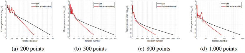
Figure 2: Convergence comparison between the original EM (black line) and the accelerated one (red line) under different point numbers. The acceleration effect becomes more significant as the number of points or the required fitting accuracy increase.

Table 1: Comparisons of different methods on noisy data, where bold font is the top fitter.

	Metric	DLS[Li and Griffiths(2004)]	HES[Kesäniemi and Virtanen(2017)]	MQF[Birdal et al.(2019)Birdal, Busam, Navab, Ilic, and Sturm]	Koop[Vajk and Hetthéssy(2003)]	Taubin[Taubin(1991)]	GF[Bektas(2015)]	RIX[López-Rubio et al.(2017)López-Rubio, Thurnhofer-Hemsi, de Cózar-Macías, Blázquez-Parra, Muñoz-Pérez, and de Guevara-López]	Ours
5	$E_{\mathbf{c}}$	3.43	3.42	3.47	4.06	3.89	1.31	0.67	1.03
	$E_{\mathbf{a}}$	0.45	0.46	0.57	0.74	0.63	0.14	0.15	0.14
10	$E_{\mathbf{c}}$	3.92	3.90	4.14	5.20	4.83	1.90	1.17	1.33
	$E_{\mathbf{a}}$	0.47	0.48	0.65	0.88	0.71	0.21	0.23	0.20
15	$E_{\mathbf{c}}$	4.51	4.49	4.11	6.12	5.87	2.14	1.66	1.58
	$E_{\mathbf{a}}$	0.48	0.49	0.76	1.11	0.86	0.29	0.29	0.25
20	$E_{\mathbf{c}}$	4.61	4.60	3.62	7.83	6.86	3.23	2.20	2.01
	$E_{\mathbf{a}}$	0.46	0.47	0.84	1.43	0.94	0.53	0.33	0.32
25	$E_{\mathbf{c}}$	4.85	4.84	5.10	8.97	8.81	4.21	2.68	2.16
	$E_{\mathbf{a}}$	0.44	0.46	1.09	1.65	1.18	0.94	0.38	0.40

Effect of the $\varepsilon$ technique. First, we reveal the effect of $\varepsilon$-accelerated EM for 200, 500, 800, and 1,000 data points. The results are reported in Fig. 2, where some observations can be drawn: (1) for the fixed point number, the acceleration effect is more significant as the required convergence accuracy increases; (2) conversely, for fixed accuracy, the acceleration effect is also more significant as the point number increases. Therefore, the $\varepsilon$ technique can effectively speed up the convergence of the ellipsoid fitting process, especially for points with a large magnitude under a high accuracy fitting requirement.

Effect of noise. Next, we add different Gaussian noise with zero mean and standard deviation $\sigma\in[5\%,25\%]$ to 200 data points. The average offset and shape deviations $E_{\mathbf{c}}$ and $E_{\mathbf{a}}$ are reported in Table 1. As observed, our fit attains the overall best performance and is more robust when heavier noise is added. GF has minor deviations than the other LS-based methods. However, when noise goes up, see $\sigma>20\%$, a significant error exists, indicating its instability for severe noise. Koop attains the largest deviations among all methods, while DLS and HES share quite similar performance. As a robust method, RIX achieves the second-best performance, but with noise increasing, such as $\sigma>15\%$, it results in more offset errors than ours. Ellipsoid fitting examples are presented in the left panel of Fig. 3.

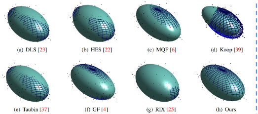
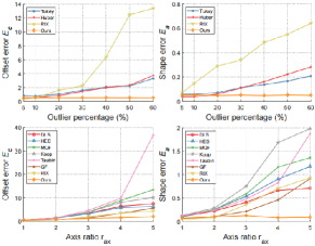
Figure 3: Left: Fitting results under 10% Gaussian noise and 1% outliers (net ellipsoid is the ground truth); right: Our method exhibits higher robustness against outliers and axis ratio.

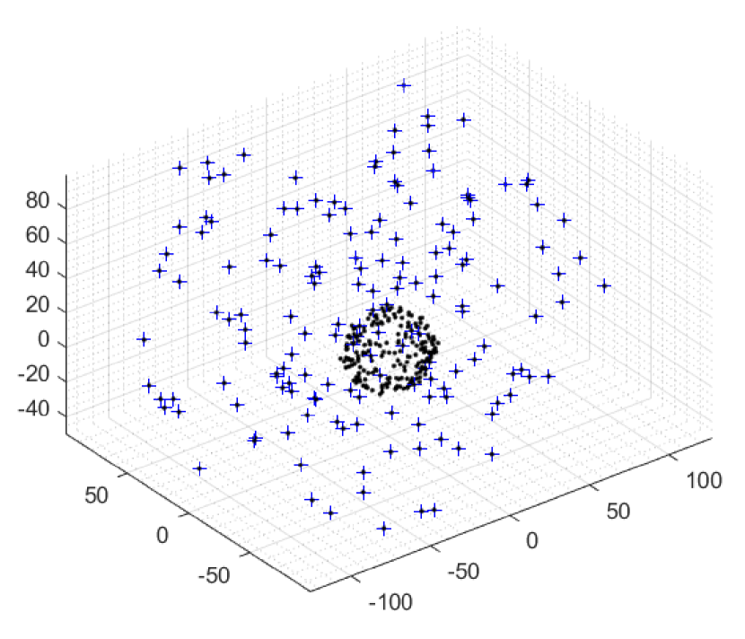
(a) Input

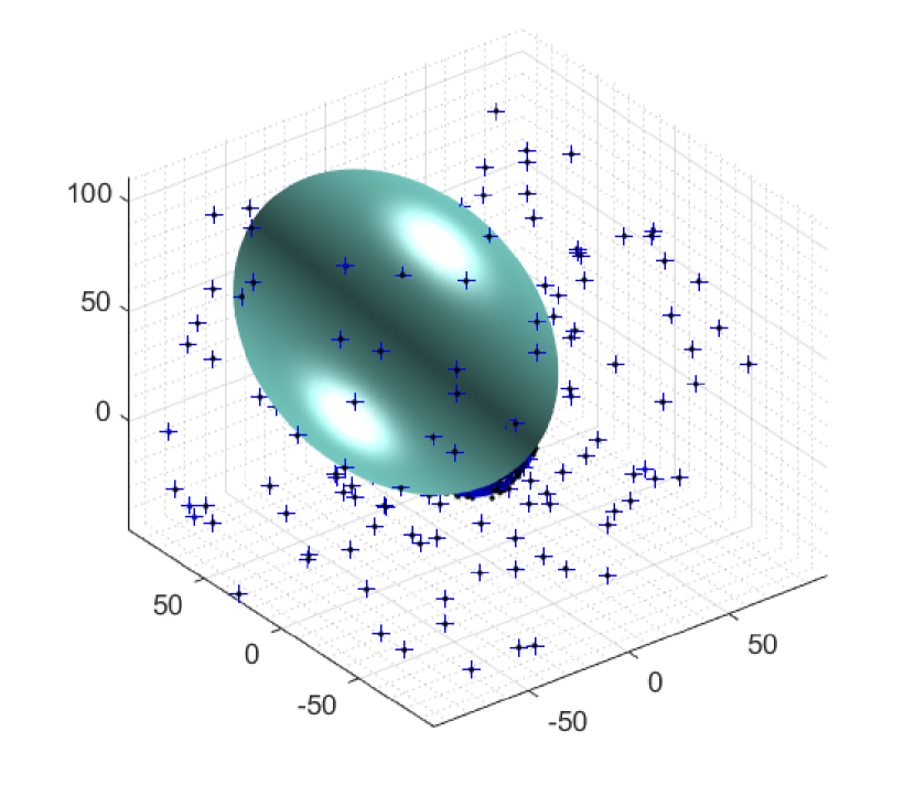
(b) Tukey [Rousseeuw(1991)]

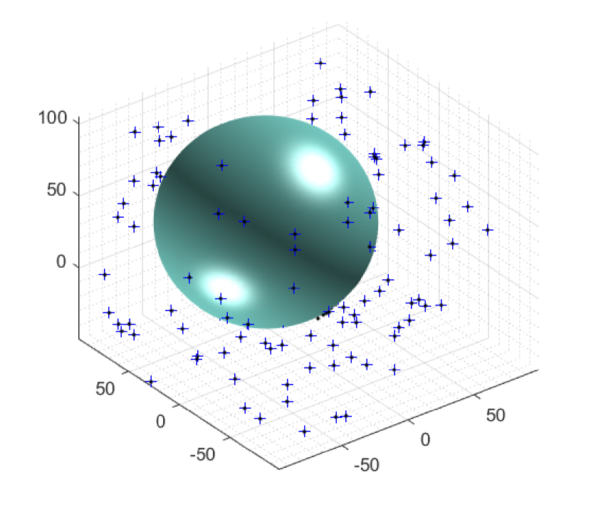
(c) Huber [Huber(2004)]

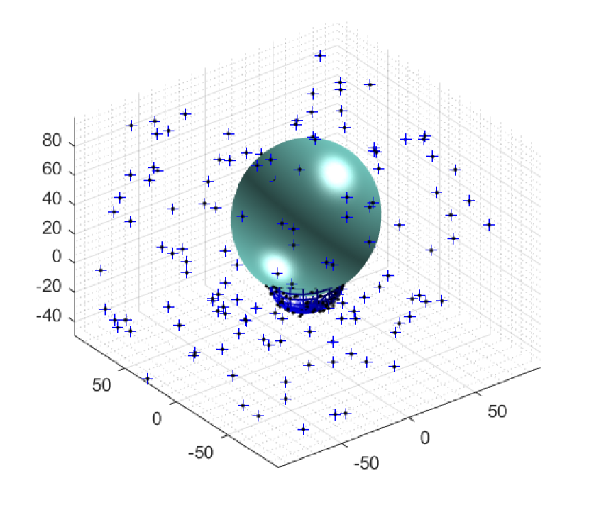
(d) RIX [López-Rubio et al.(2017)López-Rubio, Thurnhofer-Hemsi, de Cózar-Macías, Blázquez-Parra, Muñoz-Pérez, and de Guevara-López]

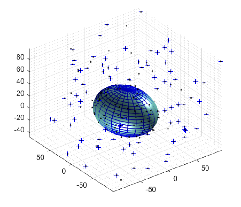
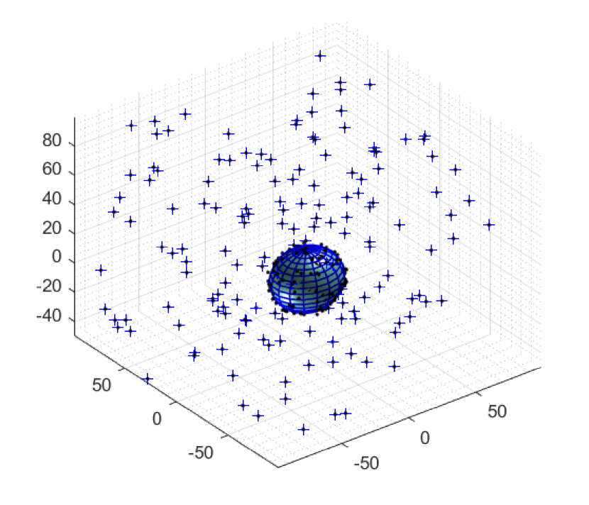
(e) Ours

Figure 4: Ellipsoid fitting examples in the presence of outliers (’+’). As outliers increase from 60% (first row) to 80% (second row), the proposed method outperforms M-estimators of Tukey and Huber, and RIX with higher robustness.

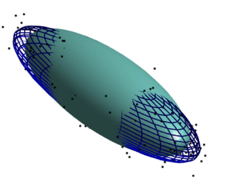
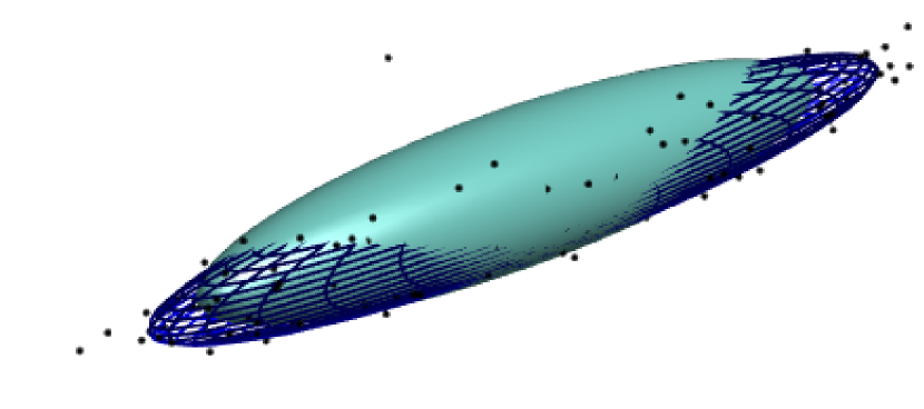
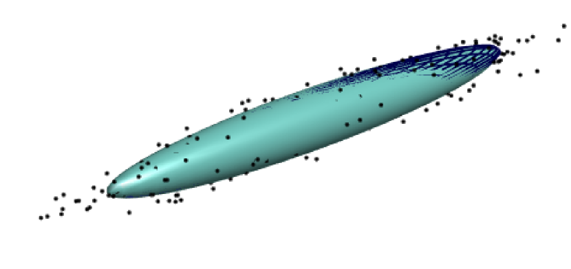
(a) DLS [Li and Griffiths(2004)]

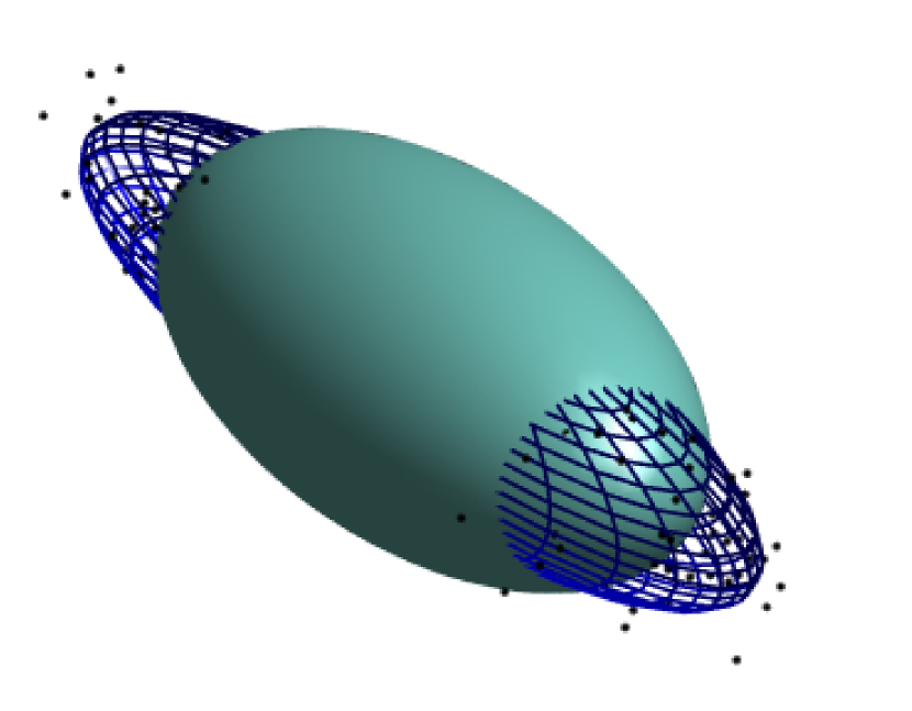
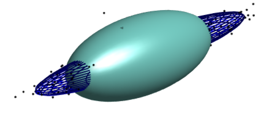
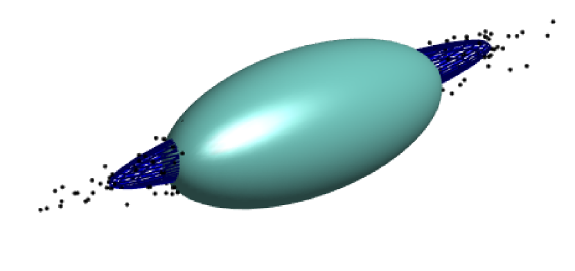
(b) HES [Kesäniemi and Virtanen(2017)]

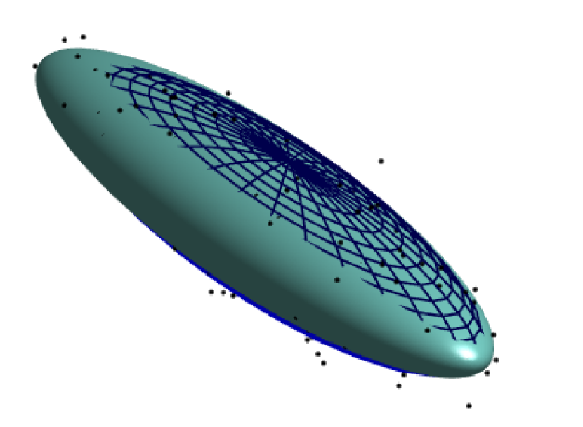
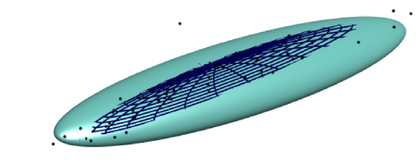
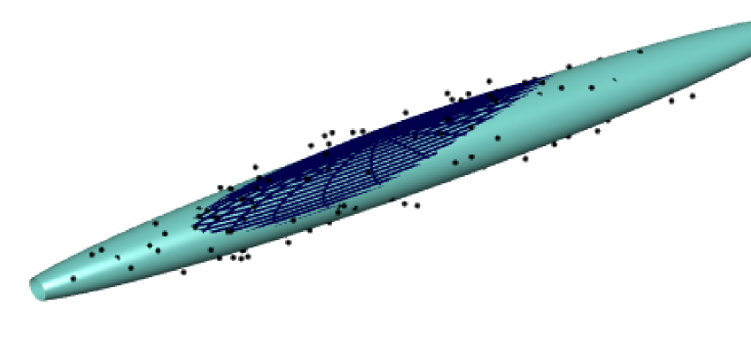
(c) MQF [Birdal et al.(2019)Birdal, Busam, Navab, Ilic, and Sturm]

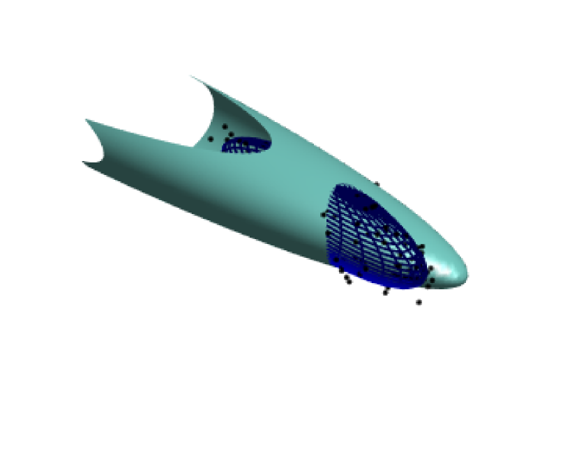
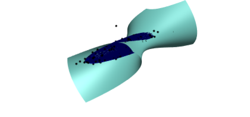
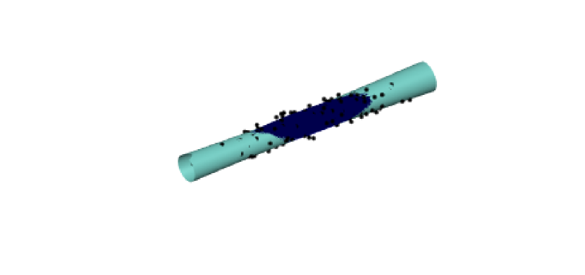
(d) Koop [Vajk and Hetthéssy(2003)]

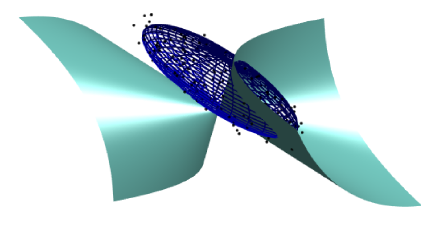
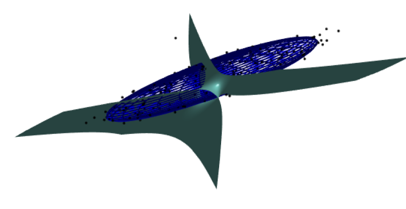
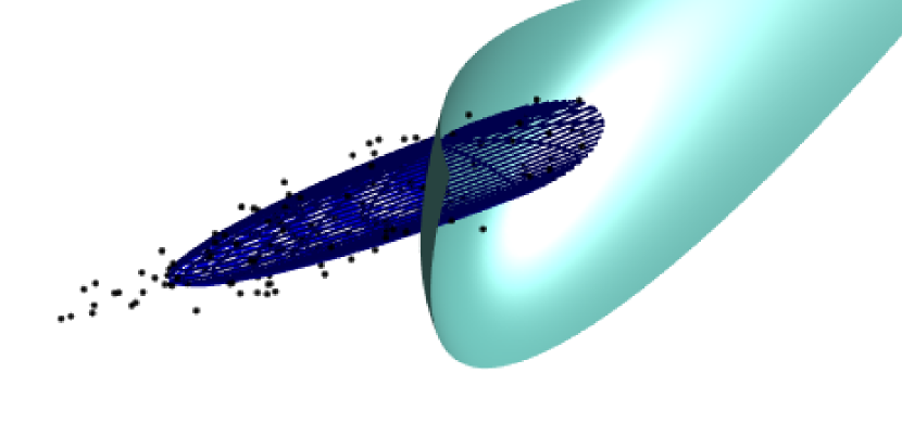
(e) Taubin [Taubin(1991)]

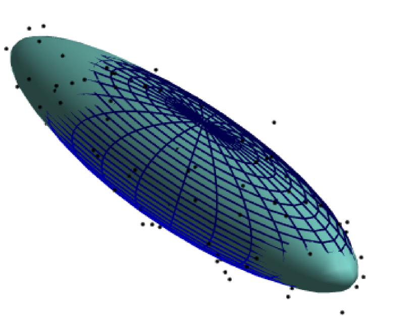
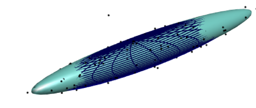
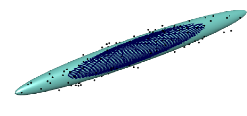
(f) GF [Bektas(2015)]

(g) RIX [López-Rubio et al.(2017)López-Rubio, Thurnhofer-Hemsi, de Cózar-Macías, Blázquez-Parra, Muñoz-Pérez, and de Guevara-López]

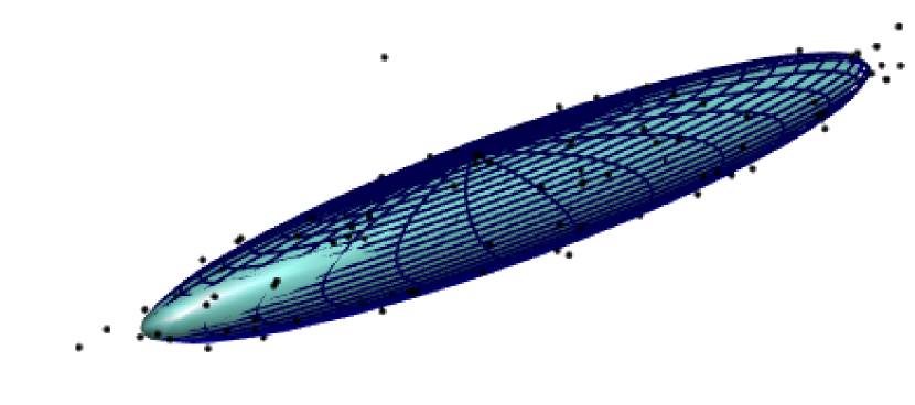
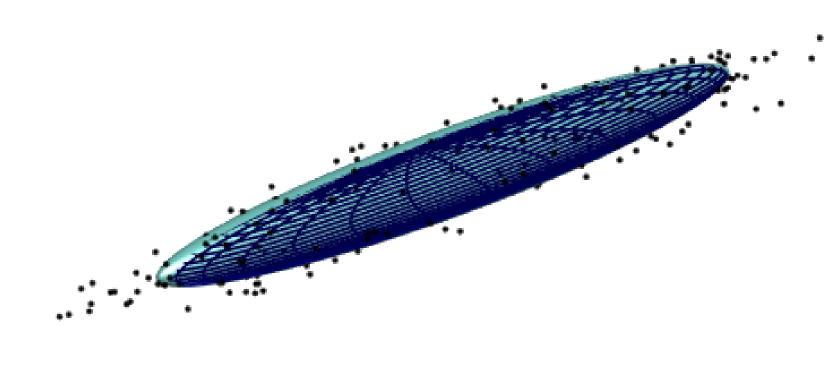
(h) Ours

Figure 5: Influence of axis ratio $r_{ax}$ to different methods. Algebraic methods return significant errors, revealing their instability for thin or flat ellipsoids. Our method attains ellipsoid-specific fittings with the highest accuracy and is more robust against axis ratio.

Effect of outliers. Subsequently, we contaminate the ground truth data by a series of outliers from $5\%$ to $60\%$, along with zero-mean Gaussian noise, and $\sigma=5\%$. Given that LS-based methods are susceptible to outliers, we test the two robust methods and the iteratively re-weighted least-squares that use two M-estimators (robust kernels), such as Tukey [Rousseeuw(1991)] and Huber [Huber(2004)]. The results in the top right panel of Fig. 3 show that RIX is relatively sensitive to outliers, especially when the outlier percentage exceeds $30\%$, which is consistent with the results reported by the authors [López-Rubio et al.(2017)López-Rubio, Thurnhofer-Hemsi, de Cózar-Macías, Blázquez-Parra, Muñoz-Pérez, and de Guevara-López]. M-estimators of Tukey and Huber have similar performance and are more robust than RIX, rooting from their weighting schemes for different residuals. Nevertheless, with outliers increasing at $60\%$, they also generate more fitting deviations. In contrast, the proposed method works fairly well, and the deviations are kept quite low and stable, even when outliers rise up to $60\%$, demonstrating its high robustness. Comparison examples are presented in Fig. 4.

Effect of the axis ratio. We also investigate the influence of the axis ratio $r_{ax}$ for ellipsoid fitting given that many existing ellipsoid-specific approaches require a prior or have limitations for axis ratio. We randomly generate a set of ellipsoids with $r_{ax}$ from 1 to 5 and the statistical results are reported in the bottom right panel of Fig. 3. As observed, except our method, the others produce significant deviations with $r_{ax}$ increasing. Taubin and Koop are more sensitive to $r_{ax}$, MQF also showing its weakness. RIX exhibits noticeable shape deviations, whereas the proposed method achieves the highest accuracy for both metrics and keeps them greatly stable. Note that we have excluded non-ellipsoid fittings in the statistic. Three randomly generated ellipsoids with $r_{ax}=5,8,10$ (from top to bottom) and corresponding fittings are shown in Fig. 5.

Ablation study of RDOS. RDOS is used to adaptively initialize the weight $w=\frac{\#\{\mathbf{x}_{i}|{\mathop{\mathrm{RDOS}}}(\mathbf{x}_{i})>2\}}{N}$ that balances GMM and the uniform distribution because $w$ influences the performance and setting it manually may bring significant deviations. We conduct an ablation study by tuning different $w$ for two outlier-contaminated cases (120 and 200 outliers). Results in the top left panel of Fig. 6 show that, compared with the random setting of $w\in\{0,0.1,0.5,0.9\}$, $w-{\mathop{\mathrm{RDOS}}}$ ($w$ estimated by ${\mathop{\mathrm{RDOS}}}$) can provide more reasonable initialization, leading to an overall higher accuracy. Meanwhile, $M=\sum_{\mathbf{x}_{i}\in\mathbf{X}}\mathbbm{1}({\mathop{\mathrm{RDOS}}}(\mathbf{x}_{i})\leq 2)$ is taken to model sphere points. We also report the effect of $M$ for the previous two cases by fixing $w=0.375,0.5$, respectively. Results in the bottom left panel of Fig. 6 indicate that more deviations will emerge if $M$ is much less than the number of inliers. On the contrary, $M-{\mathop{\mathrm{RDOS}}}$ ($M$ estimated by ${\mathop{\mathrm{RDOS}}}$) attains more satisfactory performance. Another simple choice is let $M=N$ directly, but this choice will make $w=0$ in our method, resulting in significant errors. Despite we can tune $M$ by multiples of $N$ such as $\frac{N}{2}$, it may expand efforts to find a suitable value. Thus, we use adaptive ${\mathop{\mathrm{RDOS}}}$ for weight initialization and ellipsoid modeling, simultaneously.

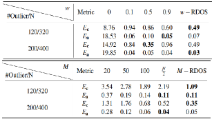
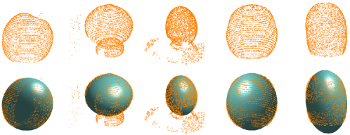
Figure 6: Left: Ablation study of RDOS for the initialization of weight $w$ (top) and the estimation of the inlier amount $M$ (bottom). Bold font indicates the top fitter; right: Our method attains successful fittings for point clouds with outliers and occlusion.

Real-world scanned point clouds. We next apply our method to 3D point clouds captured by a laser Picza scanner [López-Rubio et al.(2017)López-Rubio, Thurnhofer-Hemsi, de Cózar-Macías, Blázquez-Parra, Muñoz-Pérez, and de Guevara-López]. To boost fitting, we perform downsampling over the data (sampling rate $[0.2,0.4]$), and there are $4,000\sim 10,000$ points of each model. As shown in the right panel of Fig. 6, these point clouds bear evident occlusion or outliers that are usually disastrous for LS-based methods. However, our fits exhibit acceptable results in the sense that the ellipsoid surfaces approximate the objects well, by which metrics such as volume and direction can be estimated. Thereby, the proposed method in general is quite suited to densely sampled points attained by laser scanners or similar technologies.

6 Discussion and Conclusion

We have presented a robust and accurate method for ellipsoid-specific fitting in noisy/outlier-contaminated 3D scenes. We use GMM to model the ellipsoid explicitly and cast it in an MLE, which is effectively solved via the $\varepsilon$-accelerated EM framework. Furthermore, a uniform distribution is added to depress outliers, and all parameters are updated automatically. Comprehensive evaluations show that our method outperforms the compared ones by a large margin, especially for noisy, outlier-contaminated, ellipsoid-specific, and large axis ratio cases.

Given that our model is non-convex, EM may fall into local minima, but we scarcely see in previous experiments which may benefit from the proper initialization by RDOS. The number of mixture components in GMM depends on the measurement points, aiming to approximate arbitrary distribution. For efficiency, in future work, we can trim components based on the Gaussian bandwidth $h$ to let GMM adaptively model the ellipsoid. Furthermore, we can explore the use of a single analytic distribution over the surface of an ellipsoid for higher efficiency. Besides, we can replace Gaussian distribution by Student’s t distribution [Peel and McLachlan(2000)] to make the model more robust against noise with a heavy tail.

The proposed method can be generalized to fit other quadrics or conics, such as planes and cylinders, given the existence of a parametric representation. We give a glance at other quadric fittings in the supplemental material. Additionally, we can boost the fitting accuracy by encapsulating more geometric features like normals and curvatures into the model.

References

- [Ahn et al.(2002)Ahn, Rauh, Cho, and Warnecke] Sung Joon Ahn, Wolfgang Rauh, Hyung Suck Cho, and H-J Warnecke. Orthogonal distance fitting of implicit curves and surfaces. IEEE Transactions on Pattern Analysis and Machine Intelligence, 24(5):620–638, 2002.
- [Allaire et al.(2007)Allaire, Jacq, Burdin, Roux, and Couture] Stéphane Allaire, Jean-José Jacq, Valérie Burdin, Christian Roux, and Christine Couture. Type-constrained robust fitting of quadrics with application to the 3D morphological characterization of saddle-shaped articular surfaces. In IEEE 11th International Conference on Computer Vision, pages 1–8, 2007.
- [Beale et al.(2016)Beale, Yang, Campbell, Cosker, and Hall] Daniel Beale, Yong-Liang Yang, Neill Campbell, Darren Cosker, and Peter Hall. Fitting quadrics with a bayesian prior. Computational Visual Media, 2(2):107–117, 2016.
- [Bektas(2015)] Sebahattin Bektas. Least squares fitting of ellipsoid using orthogonal distances. Boletim de Ciências Geodésicas, 21(2):329–339, 2015.
- [Bentley(1975)] Jon Louis Bentley. Multidimensional binary search trees used for associative searching. Communications of the ACM, 18(9):509–517, 1975.
- [Birdal et al.(2019)Birdal, Busam, Navab, Ilic, and Sturm] Tolga Birdal, Benjamin Busam, Nassir Navab, Slobodan Ilic, and Peter Sturm. Generic primitive detection in point clouds using novel minimal quadric fits. IEEE Transactions on Pattern Analysis and Machine Intelligence, 42(6):1333–1347, 2019.
- [Bischoff and Kobbelt(2002)] Stephan Bischoff and Leif Kobbelt. Ellipsoid decomposition of 3D-models. In Proceedings of First International Symposium on 3D Data Processing Visualization and Transmission, pages 480–488, 2002.
- [Bishop(2006)] Christopher M Bishop. Pattern Recognition and Machine Learning. 2006.
- [Blane et al.(2000)Blane, Lei, Civi, and Cooper] Michael M Blane, Zhibin Lei, Hakan Civi, and David B Cooper. The 3L algorithm for fitting implicit polynomial curves and surfaces to data. IEEE Transactions on Pattern Analysis and Machine Intelligence, 22(3):298–313, 2000.
- [Calafiore(2002)] Giuseppe Calafiore. Approximation of n-dimensional data using spherical and ellipsoidal primitives. IEEE Transactions on Systems, Man, and Cybernetics-Part A: Systems and Humans, 32(2):269–278, 2002.
- [Faber and Fisher(2001)] Petko Faber and Bob Fisher. A buyer’s guide to euclidean elliptical cylindrical and conical surface fitting. In Proceedings of the 12th British Conference on Machine Vision, pages 521–530, 2001.
- [Fitzgibbon et al.(1999)Fitzgibbon, Pilu, and Fisher] Andrew Fitzgibbon, Maurizio Pilu, and Robert B Fisher. Direct least square fitting of ellipses. IEEE Transactions on Pattern Analysis and Machine Intelligence, 21(5):476–480, 1999.
- [Fitzgibbon and Fisher(1995)] Andrew W. Fitzgibbon and Robert B. Fisher. A buyer’s guide to conic fitting. In Proceedings of the 6th British Conference on Machine Vision, pages 513–522, 1995.
- [Gander et al.(1994)Gander, Golub, and Strebel] Walter Gander, Gene H Golub, and Rolf Strebel. Least-squares fitting of circles and ellipses. BIT Numerical Mathematics, 34(4):558–578, 1994.
- [Georgiev et al.(2016)Georgiev, Al-Hami, and Lakaemper] Kristiyan Georgiev, Motaz Al-Hami, and Rolf Lakaemper. Real-time 3D scene description using spheres, cones and cylinders. arXiv preprint arXiv:1603.03856, 2016.
- [Gietzelt et al.(2013)Gietzelt, Wolf, Marschollek, and Haux] Matthias Gietzelt, Klaus-Hendrik Wolf, Michael Marschollek, and Reinhold Haux. Performance comparison of accelerometer calibration algorithms based on 3D-ellipsoid fitting methods. Computer Methods and Programs in Biomedicine, 111(1):62–71, 2013.
- [Harris and Stöcker(1998)] John W Harris and Horst Stöcker. Handbook of mathematics and computational science. 1998.
- [Hartley(1997)] Richard I Hartley. In defense of the eight-point algorithm. IEEE Transactions on Pattern Analysis and Machine Intelligence, 19(6):580–593, 1997.
- [Huber(2004)] Peter J Huber. Robust statistics, volume 523. 2004.
- [Jia et al.(2011)Jia, Choi, Mourrain, and Wang] Xiaohong Jia, Yi-King Choi, Bernard Mourrain, and Wenping Wang. An algebraic approach to continuous collision detection for ellipsoids. Computer Aided Geometric Design, 28(3):164–176, 2011.
- [Joyce(2003)] James Joyce. Bayes’ theorem. 2003.
- [Kesäniemi and Virtanen(2017)] Martti Kesäniemi and Kai Virtanen. Direct least square fitting of hyperellipsoids. IEEE Transactions on Pattern Analysis and Machine Intelligence, 40(1):63–76, 2017.
- [Li and Griffiths(2004)] Qingde Li and John G Griffiths. Least squares ellipsoid specific fitting. In Geometric Modeling and Processing, pages 335–340, 2004.
- [Lin and Huang(2015)] Zhouchen Lin and Yameng Huang. Fast multidimensional ellipsoid-specific fitting by alternating direction method of multipliers. IEEE Transactions on Pattern Analysis and Machine Intelligence, 38(5):1021–1026, 2015.
- [López-Rubio et al.(2017)López-Rubio, Thurnhofer-Hemsi, de Cózar-Macías, Blázquez-Parra, Muñoz-Pérez, and de Guevara-López] Ezequiel López-Rubio, Karl Thurnhofer-Hemsi, Óscar David de Cózar-Macías, Elidia Beatriz Blázquez-Parra, José Muñoz-Pérez, and Isidro Ladrón de Guevara-López. Robust fitting of ellipsoids by separating interior and exterior points during optimization. Journal of Mathematical Imaging and Vision, 58(2):189–210, 2017.
- [Miller(1988)] James R Miller. Analysis of quadric-surface-based solid models. IEEE Computer Graphics and Applications, 8(1):28–42, 1988.
- [Moon(1996)] Todd K Moon. The expectation-maximization algorithm. IEEE Signal Processing Magazine, 13(6):47–60, 1996.
- [Myronenko and Song(2010)] Andriy Myronenko and Xubo Song. Point set registration: Coherent point drift. IEEE Transactions on Pattern Analysis and Machine Intelligence, 32(12):2262–2275, 2010.
- [Nikolaos Kyriazis and Argyros(2011)] Iason Oikonomidis Nikolaos Kyriazis and Antonis Argyros. Efficient model-based 3D tracking of hand articulations using kinect. In Proceedings of the 22th British Conference on Machine Vision, pages 1–11, 2011.
- [Peel and McLachlan(2000)] David Peel and Geoffrey J McLachlan. Robust mixture modelling using the t distribution. Statistics and computing, 10(4):339–348, 2000.
- [Rimon and Boyd(1997)] Elon Rimon and Stephen P Boyd. Obstacle collision detection using best ellipsoid fit. Journal of Intelligent and Robotic Systems, 18(2):105–126, 1997.
- [Rousseeuw(1991)] Peter J Rousseeuw. Tutorial to robust statistics. Journal of chemometrics, 5(1):1–20, 1991.
- [Rousseeuw and Leroy(2005)] Peter J Rousseeuw and Annick M Leroy. Robust regression and outlier detection, volume 589. John wiley & sons, 2005.
- [Sampson(1982)] Paul D Sampson. Fitting conic sections to very scattered data: An iterative refinement of the bookstein algorithm. Computer Graphics and Image Processing, 18(1):97–108, 1982.
- [Tang and He(2017)] Bo Tang and Haibo He. A local density-based approach for outlier detection. Neurocomputing, 241:171–180, 2017.
- [Tasdizen(2001)] Tolga Tasdizen. Robust and repeatable fitting of implicit polynomial curves to point data sets and to intensity images. PhD thesis, Brown university, 2001.
- [Taubin(1991)] Gabriel Taubin. Estimation of planar curves, surfaces, and nonplanar space curves defined by implicit equations with applications to edge and range image segmentation. IEEE Transactions on Pattern Analysis and Machine Intelligence, (11):1115–1138, 1991.
- [Thurnhofer-Hemsi et al.(2020)Thurnhofer-Hemsi, López-Rubio, Blázquez-Parra, Ladrón-de Guevara-Muñoz, and de Cózar-Macias] Karl Thurnhofer-Hemsi, Ezequiel López-Rubio, Elidia Beatriz Blázquez-Parra, M Carmen Ladrón-de Guevara-Muñoz, and Óscar David de Cózar-Macias. Ellipse fitting by spatial averaging of random ensembles. Pattern Recognition, 106:107406, 2020.
- [Vajk and Hetthéssy(2003)] István Vajk and Jenö Hetthéssy. Identification of nonlinear errors-in-variables models. Automatica, 39(12):2099–2107, 2003.
- [Wang et al.(2008)Wang, Kuroda, Sakakihara, and Geng] Mingfeng Wang, Masahiro Kuroda, Michio Sakakihara, and Zhi Geng. Acceleration of the em algorithm using the vector epsilon algorithm. Computational Statistics, 23(3):469–486, 2008.
- [Ying et al.(2012)Ying, Yang, and Zha] Xianghua Ying, Li Yang, and Hongbin Zha. A fast algorithm for multidimensional ellipsoid-specific fitting by minimizing a new defined vector norm of residuals using semidefinite programming. IEEE Transactions on Pattern Analysis and Machine Intelligence, 34(9):1856–1863, 2012.
- [Zhao et al.(2021)Zhao, Jia, Fan, Liang, and Yan] Mingyang Zhao, Xiaohong Jia, Lubin Fan, Yuan Liang, and Dong-Ming Yan. Robust ellipse fitting using hierarchical Gaussian mixture models. IEEE Transactions on Image Processing, 30:3828–3843, 2021.