Non-dispersive one-way signal amplification in sonic metamaterials

Abstract

Parametric amplification—injecting energy into waves via periodic modulation of system parameters—is typically restricted to specific multiples of the modulation frequency. However, broadband parametric amplification can be achieved in active metamaterials which allow local parameters to be modulated both in space and in time. Inspired by the concept of luminal metamaterials in optics, we describe a mechanism for one-way amplification of sound waves across an entire frequency band using spacetime-periodic modulation of local stiffnesses in the form of a traveling wave. When the speed of the modulation wave approaches that of the speed of sound in the metamaterial—a regime called the sonic limit—nearly all modes in the forward-propagating acoustic band are amplified, whereas no amplification occurs in the reverse-propagating band. To eliminate divergences that are inherent to the sonic limit in continuum materials, we use an exact Floquet-Bloch approach to compute the dynamic excitation bands of discrete periodic systems. We find wide ranges of parameters for which the amplification is nearly uniform across the lowest-frequency band, enabling amplification of wavepackets while preserving their speed, shape, and spectral content. Our mechanism provides a route to designing acoustic metamaterials which can propagate wave pulses without losses or distortion across a wide range of frequencies.

I Introduction

Parametric amplification—feeding energy into oscillatory modes through a periodic modulation of the underlying stiffness or coupling parameters—provides a technologically-relevant route to boosting signals and overcoming losses in electromagnetic [1, 2], optical [3] and mechanical [4] systems. Typically, parametric amplification occurs only for a discrete set of modes which satisfy specific frequency relationships with the modulation frequency [5], which obstructs its use to amplify propagating signals with multiple frequency components such as localized wavepackets. However, when the parameter modulation is itself a traveling wave through the medium, interference effects enable amplification over a wide range of signal frequencies with a single modulation frequency [6, 7], opening up possibilities for amplification and loss-compensation of multispectral signals as long as the desired spacetime parameter modulation can be achieved.

Active metamaterials—artificial structures whose properties can be modulated using external fields [8, 9, 10]—provide a promising platform for broadband parametric amplification using traveling waves [11]. In the realm of acoustics, traveling-wave modulation of elastic stiffnesses has primarily been used to achieve nonreciprocal transport [12, 13, 14, 15, 16, 17, 18], although parametric amplification has also been observed albeit in narrow frequency ranges [13]. Despite rapid developments in active acoustic metamaterial platforms which enable on-demand spatiotemporal modulation of acoustic parameters across a wide range of length and frequency scales [9, 19], traveling-wave parametric amplification remains unexploited as a mechanism to boost multispectral signals in active acoustic metamaterials.

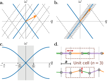
Figure 1: Sonic metamaterials. a, A 1D continuum system displays a linear dispersion relation for sound waves (solid lines). When the local stiffness $k(x,t)$ is modulated according to a traveling wave, $k(x,t)=k_{0}[1+\delta\cos(gx-\Omega t)]$, the resulting normal modes arise from the coupling of the unmodulated modes with their harmonic replicas (dashed lines) displaced by integer multiples of the vector $(g,\Omega)$ (arrow) in the frequency-wavevector plane. Here, $\Omega/g=0.4v$. b, Same as a with $\Omega/g=0.9v$. The first six harmonics are shown. As $\Omega/g\to v$, all harmonics overlap along $\omega=vq$. c, A periodic spring-mass chain with lattice spacing $a$ has a nonlinear dispersion relation across the Brillouin zone. Shaded region shows the reduced Brillouin zone when spring constants are modulated as shown in d. d, (top) Section of an infinite spring chain with lattice spacing $a$; horizontal displacements (arrow) from equilibrium (dashed vertical lines) are coupled by a repeating set of three unique spring constants (colors) as defined by Eq. (2) with $n=3$. (bottom) The same equation of motion is obeyed by vertical displacements of masses restricted to slide along immobile rigid bars spaced by $a$ (solid vertical lines) and coupled by tensed strings whose tensions (colors) are modulated according to Eq. (2).

Here, we show that a traveling-wave stiffness modulation can generate broadband parametric amplification in acoustic systems as a consequence of instabilities that arise when the speed of the traveling-wave modulation is close to the speed of sound in the medium [20, 21, 22]—a situation termed the sonic limit [6]. In the sonic limit, approximate techniques such as coupled-mode theory and plane-wave expansions, commonly used to compute the response of time-modulated metamaterials [23, 24, 25, 26], are known to break down [22, 6]. Instead, we develop a Floquet-Bloch technique to calculate the exact dispersion relation of a discrete system of masses connected by springs with spacetime-modulated stiffnesses. We find that the acoustic gain (the imaginary part of the complex frequency) can be made nearly constant over a broad range of frequencies and quasimomenta, allowing coherent amplification and loss-mitigation of acoustic signals with a broad spectral content. The gain is controlled by the modulation strength, which allows our technique to be dynamically tuned to produce the desired amplification, or to finely balance losses for unattenuated sound transmission. It is also strongly directional, allowing highly non-reciprocal response with amplified transport of signals in one direction and strong attenuation in the opposite direction. As a technologically-relevant illustration of our approach, we demonstrate dispersion-free amplification and loss-compensation of propagating wave pulses in modulated spring-mass chains.

The physical mechanism underlying the sonic limit is illustrated in Fig. 1 for a continuum one-dimensional (1D) system which admits a linear dispersion relation $\omega(q)=\pm vq$ between the inverse wavelength, or quasimomentum, $q$ of traveling waves and their oscillation frequency $\omega$ when the underlying stiffness constants are uniform [6, 11]. If the stiffness is perturbed by a periodic traveling-wave modulation with quasimomentum $g$ and frequency $\Omega$, Floquet-Bloch theory dictates that the original normal modes become strongly coupled with harmonics that are displaced by integer multiples of the vector $(g,\Omega)$ on the quasimomentum-frequency plane (Fig. 1a). When $\Omega/g$ approaches the speed of sound $v$, all harmonics of the original set of modes begin to overlap along the branch $\omega=vq$ (Fig. 1b), signifying a pile-up of harmonic contributions at the sonic limit of the modulated medium. Because of these overlapping contributions from a technically infinite set of harmonics, calculations of the dispersion relation of the infinite continuum system do not converge [6]. However, the response of a finite system over finite time intervals can still be computed, and has been shown to exhibit broadband amplification and high-frequency harmonic generation in optical metamaterials where the analogous situation has been termed the luminal limit [11].

II Floquet-Bloch band structures of time-modulated spring networks

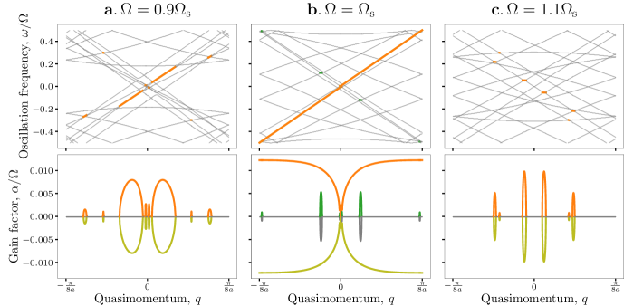
Figure 2: Floquet-Bloch complex band structures near the sonic limit. Real (top) and imaginary (bottom) components of Floquet quasifrequencies as a function of crystal quasimomentum for a system with $n=8$ and a traveling-wave modulation of $\delta=0.18$, at three different modulation frequencies (columns a–c). Floquet-Bloch analysis provides $2n=16$ complex-valued bands across the rBZ. Thin grey curves show modes with purely real frequencies, while thick curves show modes with nonzero gain or loss. The latter modes occur in pairs with identical oscillation frequencies, one of which is obscured by the other in the top row. The middle column shows a system at the sonic limit.

As an alternative to considering a system with finite extent, we avoid the divergences that plague the sonic limit by considering a discrete periodic system of masses $m$ connected by springs, whose vector of displacements $\mathbf{x}$ from equilibrium is governed by the equation of motion

$$m\mathbf{\ddot{x}}+\mathbf{K}(t)\mathbf{x}=0,$$ (1)

where $\mathbf{K}$ is the stiffness matrix (see Appendix A for the form of the matrix). Such spring-mass lattices comprise a minimal model for vibrational waves in crystals [27], and can also be used to describe effective coupled degrees of freedom in metamaterials with continuum elastic components [28, 29]. The normal modes of an infinitely long periodic chain with lattice spacing $a$ are described as continuous bands over a restricted set of unique quasimomenta $-\pi/a\leq q<\pi/a$ which defines the Brillouin zone (BZ). When all masses and springs are constant and equal, the eigenmodes of the Fourier-transformed system are organized into two bands with a nonlinear dispersion relation $\omega_{\text{s}}(q)=\pm 2\omega_{0}\sin(qa/2)$ (Fig. 1c). However, for a free-standing chain the lowest-frequency, or acoustic, band generically has a linear dispersion at low quasimomenta because translations of the structure do not stretch or compress any springs. This translational symmetry can also be replicated in anchored degrees of freedom coupled by tensile springs, which do not stretch when all points are displaced by the same amount (Fig. 1d).

We now consider the effect of sinusoidal stiffness modulations which are themselves periodic in space over a unit cell comprising $n$ degrees of freedom,

$$k_{i}(t)=k_{0}\left[1+\delta\cos\left(\frac{2\pi}{n}i-\Omega t\right)\right],$$ (2)

where $k_{i}$ is the stiffness of the $i$th coupling element along the chain, $k_{0}$ and $\delta$ are the base stiffness and the fractional amplitude of the stiffness modulation respectively, and $\Omega$ is the modulation frequency. The choice of unit cell defines a range of allowed quasimomenta or reduced Brillouin zone (rBZ) of $-\frac{\pi}{na}<k<\frac{\pi}{na}$, shown in grey in Fig. 1c. When $n$ is large, the acoustic band is effectively linear across the entire rBZ, and the sonic limit corresponds to

$$\Omega=\frac{2\pi v}{na}=\frac{2\pi}{n}\omega_{0}\equiv\Omega_{\text{s}},$$ (3)

where the speed of sound is dictated by the microscopic parameters via $v=\sqrt{k_{0}/m}a=\omega_{0}a$ with $\omega_{0}$ the natural frequency of the unmodulated springs. In the vicinity of this limit, we expect that modes over a wide range of frequencies in the lowest frequency band will experience parametric amplification due to interference with a large number of higher harmonics similar to Fig. 1b.

Since only a finite number of degrees of freedom are involved within each unit cell, the dispersion relations of the $2n$ bands (arising from the $n$ degrees of freedom per unit cell for a second-order system of differential equations) of the time-modulated system can be computed exactly using Floquet-Bloch theory without resorting to coupled-mode expansions or perturbative treatments, as described in Appendix A. The theory generates complex-valued quasifrequencies $\nu(q)=\omega(q)+i\alpha(q)$ as a function of quasimomenta $q$ in the rBZ $-\pi/(na)<q<\pi/(na)$. The real part (which can be positive or negative) sets the oscillation frequency $\omega$ of the mode, whereas the imaginary part $\alpha$ signifies exponential growth ($\alpha>0$) or decay $(\alpha<0$) of the underlying mode in time. Floquet theory dictates that every real-valued mode $\nu(q)=\omega$ is accompanied by a mode at the opposite quasimomentum with $\nu(-q)=-\omega$. For every mode with complex quasifrequency $\nu(q)=\nu_{0}$, a mode at the same quasimomentum with quasifrequency $\nu(q)=\nu_{0}^{*}$ (i.e., same oscillation frequency and gain factor with same magnitude but opposite sign) is also a solution, as are two modes at the opposite quasimomentum with $\nu(-q)=-\nu_{0}$ and $\nu(-q)=-\nu_{0}^{*}$. Furthermore, the real-valued oscillation frequencies are defined modulo $\Omega$; a minimal set of Floquet-Bloch bands is therefore defined in the range $-1/2<\omega/\Omega<1/2$.

Figure 2 shows the Floquet-Bloch bands with lowest oscillation frequency arising from the acoustic bands of a chain with $n=8$ points in the unit cell, with traveling-wave modulation frequency below, at, and above the sonic limit defined by Eq. (3). As required by the Floquet structure, modes with complex-valued quasifrequencies occur in pairs with the same oscillation frequency and opposite gain factors. Away from the sonic limit (Fig. 2a,c) complex bands occur in disconnected segments separated by quasimomenta with purely real frequencies. Exactly at the sonic limit $\Omega=\Omega_{\text{s}}$, the complex bands with constant positive slope acquire an imaginary component across the entire rBZ (Fig. 2b), with a near-constant value of the gain factor at large quasimomenta. The effect is directional: whereas the band with a positive group velocity is amplified throughout, the accompanying band with a negative slope barely experiences amplification, except in narrow quasimomentum ranges. These calculations show that unidirectional, broadband amplification of vibrations can be achieved by modulating spring stiffnesses at the sonic limit.

III Strength and parameter dependence of effect

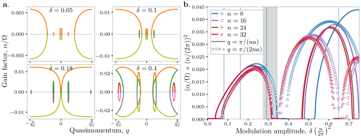
Figure 3: Parameter dependence of gain at the sonic limit. a, Gain factors (imaginary components of Floquet-Bloch bands) at $\Omega=\Omega_{\text{s}}$ for $n=8$ and varying stiffness modulation strength $\delta$. b, Largest gain factor at the band edge ($q=\pi/(na)$, solid lines) and halfway between the origin and the band edge ($q=\pi/(2na)$, symbols) as a function of modulation strength for different unit cell sizes $n$. Both quantities are scaled by the parameter $(\Omega_{\text{s}}/\omega_{0})^{2}=(2\pi/n)^{2}$ which sets the strength of parametric amplification in the system. Vertical dashed lines indicate the four values of the modulation strength for the $n=8$ bands in a. In the shaded region, the gain factors at wavevectors $\pi/(na)$ and $\pi/(2na)$ coincide, consistent with broadband amplification of near-constant strength across much of the rBZ.

While a near-constant gain factor can be attained across much of the Brillouin zone in the sonic limit, this is not guaranteed at all modulation strengths. The nonlinear dispersion relation of the unmodulated system, and the presence of additional bands that accidentally satisfy resonance conditions with the traveling-wave modulation, together generate a rich structure of complex Floquet-Bloch bands at the sonic limit. Figure 3a shows how the gain factors vary with modulation strength $\delta$ at the sonic limit for a unit cell with $n=8$. At low modulation strengths, a region of nonzero gain opens up in the lowest-frequency band with positive slope around the band edges $q=\pm\pi/(8a)$. The region expands towards the origin, creating a nearly flat gain-quasimomentum dependence across much of the rBZ at $\delta=0.18$. At higher modulation strengths, several bands acquire an appreciable gain factor in various quasimomentum ranges due to additional resonances, and the gain factors become strongly $q$-dependent.

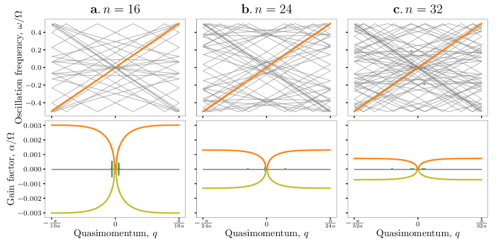
Figure A1: Floquet-Bloch band structures with $\Omega=\Omega_{\text{s}}$ and $\delta=0.27(2\pi/n)^{2}$ for different unit cell sizes. While the number of bands $2n$ grows with unit cell size, only the acoustic band with positive slope is singled out for broadband parametric amplification, with an associated gain factor that scales as $1/n^{2}$.

Despite this rich structure, at the sonic limit we can reliably find modulation strengths which realize near-constant broadband amplification. When time is scaled by the inverse of the modulation frequency $\Omega$, the Fourier-transformed dynamical matrices depend on the rescaled base stiffness $(\omega_{0}/\Omega)^{2}$ and the rescaled modulation strength $\delta(\omega_{0}/\Omega)^{2}$. At the sonic limit $\omega_{0}/\Omega=n/(2\pi)$, we expect resonances across the lowest band, whose gain factor is set by the rescaled strength $\delta(n/(2\pi))^{2}$. Calculations of the largest gain factor at the BZ edge, $q=\pi/(na)$, and halfway to the BZ center, $q=\pi/(2na)$, show that the gain factor takes on similar values at both quasimomenta for rescaled modulation strengths in the range 0.25 to 0.32 before dropping back to zero. Full Floquet-Bloch band structures for higher values of $n$ confirm near-constant gain factors across the BZ, see supplementary Fig. A1. At higher modulation strengths, additional regions of nonzero gain arise, but the gain factors differ across the band (lower right panel of Fig. 3a). These regions are reminiscent of higher-order “instability tongues” in the Mathieu equation, and arise due to additional resonances among the vibrational modes and the modulation [30]. The absence of perfect collapse of the curves at different unit cell sizes is due to the finite deviation of the lowest band from the idealized linear dispersion, which becomes smaller as $n$ increases due to the shrinking reduced Brillouin zone (Fig. 1c).

Figure 3b shows that the fractional stiffness modulation required for the strongest broadband amplification falls with increasing unit cell size, $\delta\approx 0.27(2\pi/n)^{2}$. In principle, broadband amplification can be realized even if the experimentally-achievable stiffness modulation strength is small, by increasing the wavelength of the stiffness-modulating traveling wave. However, the corresponding gain factor, which is set by the modulation strength and governs the exponential growth $\sim e^{\alpha t}$ in the signal with time, falls as $\alpha/\Omega\sim\delta\sim 1/n^{2}$ (or $\alpha/\omega_{0}\sim 1/n^{3}$). At higher stiffness modulations, the sonic limit extends over a broader range of modulation phase velocities [6], and stronger broadband amplification can be achieved with slightly slower traveling-wave modulations $\Omega\lesssim\Omega_{\text{s}}$ (see Appendix B).

IV Interplay of parametric amplification and damping

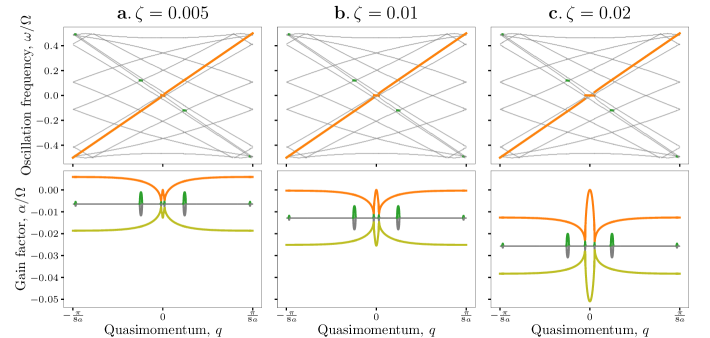
Figure 4: Effect of damping on broadband parametric amplification. Real (top) and imaginary (bottom) components of Floquet quasifrequencies as a function of crystal quasimomentum for a system with $n=8$, $\delta=0.18$, and $\Omega=\Omega_{\text{s}}$, at three different values of the damping ratio $\zeta=\gamma/(2m\omega_{0})$. In this case, modes that are not parametrically amplified have a negative gain factor $\alpha/\Omega=-\zeta\omega/\Omega=-\zeta n/(2\pi)$, signifying exponentially-damped modes, and are shown in grey. Thick colored curves show modes whose gain factors deviate from this value.

The existence of modes with positive gain factors points to the presence of instabilities—even the slightest perturbation to the system, if it overlapped with one of the amplified modes, would lead to displacements which grow exponentially in time and ultimately overcome the system. However, if the amplification can be controlled—for instance, by turning the stiffness modulation on for finite periods of time—the positive gain factors can be used to amplify modes in the system. Furthermore, in systems with damping, positive gain factors can be used to compensate for losses and propagate signals over longer distances.

We first review the effect of damping on the phonon band structure of a static spring lattice with uniform spring constants. Upon adding a drag force of the form $-\gamma\dot{\mathbf{x}}$ to the equation of motion (Eq. (1)), the frequency bands become complex-valued:

$$\omega(q)=\pm\sqrt{\omega_{\text{s}}^{2}(q)-\left(\frac{\gamma}{2m}\right)^{2}}.$$ (4)

Modes whose undamped frequency was large compared to the damping frequency scale $\gamma/m$ experience a small shift in their oscillatory frequency, and acquire a negative gain factor $\alpha=-\gamma/(2m)$. At low frequencies, however, the frequencies become purely imaginary, and the two overdamped modes decay exponentially with rate $\alpha=-\gamma/(2m)\pm\sqrt{(\gamma/(2m))^{2}-\omega_{\text{s}}^{2}}$. At $q=0$, a zero-frequency mode is guaranteed to exist, which corresponds to a displacement of all masses by the same amount at zero speed, which does not deform any springs and induces no drag forces. This mode is accompanied by another mode with $\alpha=-\gamma/m$, corresponding to all masses initially moving at the same speed.

The effect of damping on modulated structures is readily incorporated in the Floquet-Bloch eigenvalue computation, and leads to similar results to the static case. Figure 4 shows the effect of damping on the sonic metamaterial with $n=8$ reported in Fig. 2b. The damping strength is quantified by the dimensionless damping factor $\zeta\equiv\gamma/(2m\omega_{0})$. In the presence of drag forces, the symmetries between complex quasifrequences $\nu(q)$ and $\nu(-q)$ are no longer obeyed. Instead, we find that modes with large oscillation frequencies compared to $\gamma/m$ have their gain factors shifted down by roughly $\gamma/(2m)$, whereas modes near $q=0$ in the lowest band become purely imaginary. However, the near-constant value of the gain factor away from $q=0$ is maintained, showing that the broadband aspect of parametric amplification near the sonic limit is preserved in damped systems. At $\zeta=0.01$, the largest gain factor is close to zero across the entire acoustic band, signifying a balance point between the broadband parametric amplification and the drag. We will further investigate this balance, and its consequences for signal propagation, in the next section.

V Dispersion-free amplification and loss mitigation of sound pulses

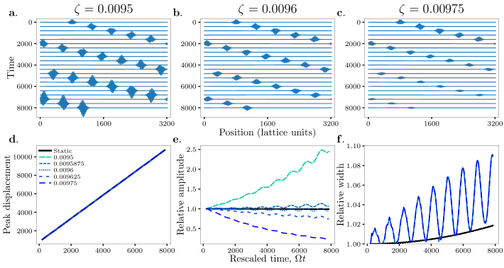
Figure 5: Pulse propagation in classical dynamics simulations of a 1D spring-mass chain at the sonic limit ($n=8$, $\delta=0.18$, $\Omega=\Omega_{\text{s}}$). a–c, Evolution of the same initial pulse in simulations with damping strength above, at, and below the balance point with the broadband parametric amplification. Curves are ordered in increasing time from top to bottom, and time advances by 10000 timesteps between successive curves. Periodic boundary conditions allow the propagating pulse to wrap around the system several times. d–f, Pulse propagation properties obtained by fitting a Gaussian lineshape to the displacement amplitudes, for different damping ratios near the balance point. d, Displacement of the pulse peak (in lattice units) as a function of time. e, Evolution of the pulse amplitude with time, relative to the intial amplitude. Solid line corresponds to an undamped system with unmodulated spring stiffnesses ($\delta=0$). f, Evolution of the pulse width over time, relative to its initial value.

To illustrate the utility of the broadband amplification mechanism for boosting signals and overcoming losses, we study the propagation of localized sound pulses (Gaussian wavepackets) along a chain of springs. Specifically, the system is initialized with a linear superposition of eigenmodes $\mathbf{\phi}_{q}$ from the acoustic band with a linear frequency-momentum relationship. The mode weights are Gaussian-distributed with spread $\Delta q$ about the mean quasimomentum $q_{0}$:

$$\mathbf{u}(n)=\sum_{q}e^{-[(q-q_{0})/\Delta q]^{2}}\boldsymbol{\phi}_{q}e^{i(qn-\omega_{q}t)},$$ (5)

where $\mathbf{u}(n)$ is the vector of initial displacements of the $n$th unit cell, $\boldsymbol{\phi}_{q}$ is the Floquet-Bloch eigenvector of the amplified band at quasimomentum $q$, and $\omega_{q}$ is the real component of the eigenfrequency. In the unmodulated and undamped static system, the resulting sound pulse propagates at a constant speed given by the slope of the linear dispersion relation, $\partial\omega/\partial k=v$ (Appendix D). In the presence of damping, however, all modes decay exponentially in time as $\sim e^{-\gamma t/(2m)}$, leading to an overall exponential decay in the pulse amplitude. When the broadband amplification is turned on, the near-constant gain compensates for the damping across most of the band, shifting the negative gain factors towards or above zero as the modulation strength is increased. Upon turning on the broadband modulation at increasing strengths, the pulse attenuation can be slowed down or even reversed to amplify the pulse as it propagates along the chain, as shown in Fig. 5. At a particular modulation strength, the net gain factors are zero across most of the acoustic band (Fig. 4b), and we expect the sound pulse to travel at constant amplitude with little dispersion, demonstrating near-ideal loss compensation through stiffness modulation.

We test this mechanism in classical dynamics simulations of a finite one-dimensional spring-mass system (see Appendix C for details) at the sonic limit, with different damping levels (Fig. 5). The spring constants were modulated according to the parameters used in Fig. 2b. A Gaussian pulse was initialized with $q_{0}=0.25/a$, $\Delta q=0.1q_{0}$ and the subsequent dynamics of the chain were simulated over thousands of stiffness modulation cycles. We find that the wavepacket travels at a constant speed, and its amplitude shows different dynamics depending on the damping strength but with minimal distortion of the pulse width or shape (Fig. 5a–c). In particular, at a specific value of the damping relative to the modulation, the pulse maintained a near-constant amplitude over long times as shown in Fig. 5b.

To assess the fidelity of the loss-compensation and amplification, we track the pulse position, amplitude, and width as a function of time by fitting a Gaussian profile to the displacement field (see Methods for details). Consistent with our theoretical expectations from the band structure calculations, we find that the wavepacket speed is not affected by the amplification level (Fig. 5d). The relative amplitude (the ratio of the pulse amplitude to its initial value) shows exponential growth, decay, or stasis as the system damping is changed. Specifically, a threshold value $\zeta=0.0096$ separates damping factors at which the pulse amplitude decreases over time from those for which the amplitude increases (Fig. 5e). At this value, damping and parametric amplification are in balance, signifying idealized loss-compensation in the system. The pulse width changes by only a few percent over thousands of cycles of the stiffness modulation (Fig. 5f). This lack of dispersion is owed to the nearly constant values of the gain factors across the band in sonic metamaterials; non-constant gain factors would lead to rapidly changing and spectral properties, as we show in Appendix D.

VI Discussion

We have shown that a traveling-wave stiffness modulation generates broadband parametric amplification of sound waves when the modulation wave speed approaches the speed of sound in the medium, confirming a recent hypothesis grounded in a similar effect for light [11]. We quantify the effect using a discrete Floquet-Bloch approach to compute complex-valued quasifrequencies without encountering divergences or requiring truncated expansions. For a broad range of parameter values, we find that the amplification factor is nearly constant over almost all quasimomenta of a particular band, which enables Gaussian wavepackets to propagate without dispersion or energy loss even in the presence of damping. The amplification is highly directional, signifying a strong nonreciprocal response in the metamaterial [19]. The mechanism could be realized in any active acoustic metamaterial with a linear dispersion relation at low quasimomenta for which the effective stiffness can be modulated in space and time, such as beams with piezoelectric [13] or electromagnetic [31] actuation, or backgated micromechanical resonator arrays [32].

Beyond signal amplification, our work suggests several avenues for future research. The presence of parametric gain in our system makes the underlying eigenvalue problem non-Hermitian. Our strategy therefore complements approaches based on active feedback to realize non-Hermitian mechanical phenomena [33, 34, 35]. The exact Floquet-Bloch framework used here is equally applicable to slow and fast time modulations, bridging the gap between theoretical approaches that rely on adiabatic (for slow modulation) or Magnus (for fast modulation) expansions and thereby enabling the exploration of non-Hermitian topological phenomena in regimes where the modulation and excitation frequencies are of similar order [36]. Higher-dimensional generalizations of the mechanism are also conceivable, since the nearly-linear dispersion relation at zero quasimomenta is guaranteed by translational symmetry.

Appendix A Floquet-Bloch band structures of spacetime-modulated spring lattices

Prior studies of spring networks with modulated stiffnesses have relied on various approximations to analyze the eigenmode structure. In the time domain, the Magnus expansion has been used [37] which relies on a separation of slow and fast frequency scales in the system. This assumption breaks down at the sonic limit, where the modulation frequency is comparable to the normal mode frequencies of the unperturbed system. Alternatively, many studies use plane-wave expansions of the spatial eigenmodes [38, 23, 24, 39, 25, 40, 41, 42, 43, 12, 44, 45, 31, 13] which must be truncated at some high wavevector to carry out actual computations. However, these approaches have been shown to be liable to inaccuracies at the sonic limit where an ever-larger number of plane waves must be included in the expansion to avoid divergences in the perturbative calculations [22, 6, 7].

To accurately predict the vibrational modes of spacetime-modulated spring lattices, we use an exact Floquet-Bloch approach which avoids perturbative expansions, albeit at the cost of requiring a numerical integration of the underlying dynamical equations over one time period. Our approach is similar to those used for driven electronic systems [46, 47], but adapted to the second-order equations of mechanics [48]. We are interested in the normal modes of a spring-mass chain of $N$ masses, whose displacements are arranged into an $N$-vector $\mathbf{x}$. When the springs are harmonic, the equation of motion is

$$m\mathbf{\ddot{x}}+\boldsymbol{\Gamma}_{N}\mathbf{\dot{x}}+\mathbf{K}(t)\mathbf{x}=0,$$ (6)

where $\boldsymbol{\Gamma}_{N}=\gamma\times\mathds{1}_{N}$ is an $N\times N$ diagonal matrix of drag coefficients (assumed uniform), and $\mathbf{K}$ is an $N\times N$ matrix of spring stiffnesses which encodes the coupling of adjacent degrees of freedom. For the 1D chain, the stiffness matrix takes the tridiagonal form

$$\mathbf{K}=\begin{pmatrix}...&...&...&...&...&...&...&...\\ ...&0&-k_{j}&k_{j}+k_{j+1}&-k_{j+1}&0&...&...\\ ...&0&0&-k_{j+1}&k_{j+1}+k_{j+2}&-k_{j+2}&0&...\\ ...&...&...&...&...&...&...&...\end{pmatrix}$$ (7)

When the spring constants $k_{j}$ are modulated in time and space according to the traveling-wave modulation

$$k_{j}(t)=k_{0}\left[1+\delta\cos\left(\frac{2\pi}{n}j-\Omega t\right)\right],$$ (8)

the eigenmodes of the dynamical system can be written in terms of an $n$-vector $\mathbf{u}_{q}(t)$ and a quasimomentum $q$, where the displacements of the $p$th unit cell at position $x=pna$ are given by $\mathbf{u}_{q}(t)e^{iqx}$. The $\mathbf{u}_{q}(t)$ solve the equation

$$m\mathbf{\ddot{u}}_{q}+\boldsymbol{\Gamma}_{n}\mathbf{\dot{u}}_{q}+\mathbf{\tilde{K}}(q,t)\mathbf{u}_{q}=0,$$ (9)

where the Fourier-transformed stiffness matrix $\mathbf{\tilde{K}}(q,t)$ has dimensions $n\times n$, and includes phase factors $e^{\pm iqna}$ for springs that extend to neighboring unit cells. For an infinite periodic lattice, the periodicity defines a unique set of quasimomenta $-\pi<qna\leq\pi$, which define the reduced Brillouin zone.

We now exploit the time-periodicity of the stiffness matrix, $\mathbf{\tilde{K}}(q,t+T)=\mathbf{\tilde{K}}(q,t)$ where $T=2\pi/\Omega$. To apply the Floquet theory of first-order differential equations, we rewrite Eq. (9) as a first-order equation involving the doubled vector $\mathbf{y}_{q}=(\mathbf{u}_{q},\mathbf{\dot{u}}_{q})^{\top}$,

$$\mathbf{\dot{y}}_{q}=\mathbf{G}_{q}(t)\mathbf{y}_{q},$$ (10)

where

$$\mathbf{G}_{q}(t)=\begin{pmatrix}0&\mathds{1}_{n}\\ -\mathbf{\tilde{K}}(q,t)&-\mathbf{\Gamma}_{n}\end{pmatrix}$$

inherits the time-periodicity of the stiffness matrix. Any solution to the differential equation can be written in terms of the matrix of solutions, $\mathbf{X}(t)$, which satisfies

$$\mathbf{\dot{X}}=\mathbf{G}_{q}(t)\mathbf{X},$$ (11)

starting from the initial condition $\mathbf{X}(0)=\mathds{1}_{2n}$. Any solution of Eq. (10) then can be written in terms of the initial condition as

$$\mathbf{x}(t)=\mathbf{X}(t)\mathbf{x}(0).$$

When $G$ is $T$-periodic, the matrix of solutions has the property

$$\mathbf{X}(t+T)=\mathbf{X}(t)\mathbf{X}(T).$$ (12)

The solution matrix evaluated over one period, $\mathbf{X}(T)$, is called the monodromy matrix. The eigenvalues $\rho_{j}$ (with $j=1,...,2n$) and corresponding eigenvectors $\mathbf{a}_{j}$ of the monodromy matrix have the following useful property: a solution $\mathbf{x}_{j}(t)$ of Eq. (10) with initial value $\mathbf{x}_{j}(0)=\mathbf{a}_{j}$ satisfies

$$\mathbf{x}_{j}(t+T)=\rho_{j}\mathbf{x}_{i}(t).$$ (13)

The eigenvalues $\rho_{j}$ are called the Floquet multipliers of the system. Equation (13) implies the form

$$\mathbf{x}_{j}(t)=e^{-i\nu_{j}t}\mathbf{f}_{j}(t),$$ (14)

where $\nu_{j}\equiv i(\ln\rho_{j})/T$ is the $i$th Floquet quasifrequency, and

$$\mathbf{f}_{j}(t)=\mathbf{X}(t)e^{-\frac{t}{T}\ln\mathbf{X}(T)}\mathbf{a}_{j}$$

is $T$-periodic by the periodicity of the matrix of solutions:

$$\mathbf{f}_{j}(t+T)=\mathbf{f}_{j}(t).$$

The $2n$ vectors $\mathbf{x}_{j}(t)$ are linearly independent and form a fundamental set of solutions of the system.

At each quasimomentum $q$, the Floquet calculation gives us $2n$ quasifrequencies $\nu_{j}(q)=\omega_{j}(q)+i\alpha_{j}(q)$; these are the Floquet-Bloch bands of the system. The calculation involves a numerical integration of Eq. (11) over one time period. Provided the numerical integration can be carried out to the desired precision, the calculation of the bands is exact as it does not rely on any truncated expansion of the solutions in terms of plane waves. The corresponding normal mode displacements and velocities of the $p$th unit cell at position $x=pna$ are written in terms of the Floquet-Bloch eigenvectors $\mathbf{f}_{j}(q,t)$ as

$$\mathbf{y}_{j}(q,t)=\mathbf{f}_{j}(q,t)e^{i[qx-\nu_{j}(q)t]}.$$ (15)

This form is similar to that of the normal modes of a static spring chain, with the differences that: i. the vector multiplying the plane-wave itself has an additional time dependence (albeit one that is $T$-periodic in time); ii. the Floquet exponents which take the place of the frequencies are in general complex-valued; iii. the oscillation frequencies $\omega_{j}=\operatorname{Re}(\nu_{j})$ are defined modulo the modulation frequency $\Omega$.

The correspondence of the Floquet-Bloch eigenmodes with normal modes of static systems is even stronger if we consider strobed measurements, i.e. when displacements are recorded only at integer multiples of the time period $T$. At these time intervals, we have

$$\mathbf{y}_{j}(q,t)=\mathbf{f}_{j}(q,0)e^{i[qx-\nu_{j}(t)]};$$

i.e. the strobed spacetime-dependence is obtained by multiplying a constant eigenvector with a plane wave. When measurements are strobed, therefore, the Floquet eigenvectors and exponents are completely analogous to the normal modes and eigenfrequencies of a static spring network. The group and phase velocities of waves in the $j$th band are determined by the dispersion relation $\omega_{j}(q)$. When the gain factor is nonzero, a positive gain factor corresponds to an exponentially growing wave amplitude $\propto e^{\alpha_{j}t}$ whereas a negative gain factor corresponds to an exponentially decaying wave.

Appendix B Sonic limit at larger modulation strengths

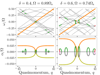
Figure A2: Broadband amplification at large modulation strengths. Floquet-Bloch band structures, similar to those in the main text, for systems with $n=8$ and two larger values of $\delta$. The sonic limit extends over a range of values around $\Omega=\Omega_{\text{s}}$ for large modulation strengths, and nearly constant gain factors are obtained at lower values of $\Omega$ compared to the limit of small $\delta$.

The accumulation of resonances which defines the sonic limit extends over a finite range of modulation frequencies on either side of the value $\Omega_{\text{s}}=2\pi v/(na)$, defined by [22, 6]

$$\frac{1}{\sqrt{1+\delta}}<\frac{\Omega}{\Omega_{\text{s}}}<\frac{1}{\sqrt{1-\delta}}.$$ (16)

In the main text, we focused on modulation frequencies at the center of this range, which is appropriate when $\delta\ll 1$. However, if larger modulation strengths are accessible, the modulation frequency that generates near-uniform gain factors across the reduced Brillouin zone can deviate from the strict sonic limit defined in Eq. (3) of the main text. In this case, modulation parameters which allow stronger broadband amplification can be found by numerically exploring Floquet-Bloch band structures within the range of values dictated by Eq. (16). As an example, Fig. A2 shows near-constant gain factors across the rBZ for $\Omega=0.89\Omega_{\text{s}}$ when $\delta=0.4$ and $\Omega=0.74\Omega_{\text{s}}$ when $\delta=0.6$, for the same unit cell size ($n=8$) discussed in Fig. 3a. In both cases, the larger modulation also enables higher gain factors to be realized compared to the case of $\Omega=\Omega_{\text{s}}$.

Appendix C Simulation methods

Wave pulse propagation in 1D spring-mass chains was studied using classical dynamic simulations implemented in the HOOMD-Blue software package [49, 50]. The system examined was a 1D spring-mass chain of $N$ particle-masses of mass $m$ possessing a unit cell of $n$ different dynamic springs with equilibrium length $l_{0}$ in a damped environment with damping constant $\gamma$. To implement dynamic springs following Eq. (2), the spring constant of each spring was updated after each time step. Simulations were initialized with a Gaussian wavepacket assembled using the Floquet-Bloch eigenvectors of the chain as described in the text (Eq. (5)). The Floquet-Bloch calculation generates both positions and velocities (Appendix A) for the initial condition.

For all simulations, we set $m=1$, $l_{0}=1$, and $k_{0}=1$ in simulation units. The spring-mass chain was created using 201 repetitions of a unit cell of $n=8$, giving rise to a system size of $N=1608$, with periodic boundary conditions along the $x$ direction. Simulations were run for $1\times 10^{8}$ time-steps with a step size $\Delta t=0.0001$. We checked that reducing the step size by a factor of 4 did not significantly change the pulse evolution with time.

The overall shape of the wavepacket was tracked during the simulation by fitting the particle displacement amplitudes to a Gaussian profile for each time snapshot. The center position, amplitude, and standard deviation of the Gaussian profile were treated as free parameters whose best-fit values were obtained using the optimize.curve_fit function from the scipy package in Python. These quantities are reported in Fig. 5 of the main text.

Appendix D Dispersion of wavepackets under non-constant gain factors

Here, we compute the distortion of Gaussian wavepackets whose constituent modes have non-uniform gain factors. For simplicity, we work with continuum plane waves of the form $e^{i[kx-\nu(k)t]}$ with momentum $k$ and a dispersion relation $\nu(k)=\omega(k)+i\alpha(k)$ relating the complex frequencies to the wavevectors. We expect the behavior of the amplitude envelope to be similar for a wavepacket built from Floquet-Bloch eigenmodes of the amplified band in the discrete system with time-modulated springs.

First, we review the effect of a nonlinear dispersion relation $\omega(k)$ on the time dynamics of a Gaussian wavepacket in the absence of gain, $\alpha(k)=0$. The wavepacket is a superposition of plane waves with weights

$$\tilde{f}(k)=A_{0}\frac{\sigma}{\sqrt{2\pi}}e^{-\frac{\sigma^{2}}{2}(k-k_{0})^{2}},$$ (17)

which leads to a real-space pulse at time $t=0$ of

$$f(x,0)=A_{0}e^{ik_{0}x}e^{-\frac{x^{2}}{2\sigma^{2}}},$$ (18)

where $A_{0}$ is the initial amplitude, and $\sigma$ is the width of the Gaussian envelope centered at $x=0$ of a sinusoidally varying wave with dominant wavevector $k_{0}$. The subsequent time-evolution is given by

$$f(x,t)=\int_{-\infty}^{\infty}\!dke^{i[kx-\omega(k)t]}\tilde{f}(k).$$

If the pulse is sufficiently broad, the Fourier amplitudes fall off fast away from $k_{0}$, and we can approximate the dispersion relation near $k_{0}$ as a Taylor series:

$$\omega(k)\approx v_{\text{p}}k_{0}+v_{\text{g}}(k-k_{0})+\frac{\eta}{2}(k-k_{0})^{2},$$

where $v_{\text{p}}=\omega(k_{0})/k_{0}$ and $v_{\text{g}}=\partial\omega(k_{0})/\partial k$ are respectively the phase and group velocity of the wave at $k_{0}$. The solution in real space at finite times is then obtained by taking the inverse Fourier transform, with the result

$$f(x,t)=A_{0}e^{i(v_{\text{g}}-v_{\text{p}})k_{0}t}e^{ik_{0}(x-v_{\text{g}}t)}e^{-\frac{(x-v_{\text{g}}t)^{2}}{2(\sigma^{2}-i\eta t)}}.$$ (19)

When the dispersion relation is strictly linear, $\eta=0$, the finite-time solution has the form $f(x,t)=e^{i(v_{\text{g}}-v_{\text{p}})k_{0}}f(x-v_{\text{g}}t,0)$, which corresponds to a translation of the Gaussian amplitude profile by $v_{\text{g}}t$ along the $x$-axis, and an additional phase factor which does not affect the amplitude (and which is zero for a linear dispersion relation $\omega=v_{\text{g}}k=v_{\text{p}}k$). The wavepacket is said to be non-dispersive, as it maintains its shape while propagating at a constant speed.

By contrast, when $\eta\neq 0$, the last exponential in Eq. (19) can be written as

$$e^{\frac{i\eta t}{2(\sigma^{4}+\eta^{2}t^{2})}}e^{-\frac{(x-v_{\text{g}}t)^{2}}{2\sigma^{2}(1+\eta^{2}t^{2}/\sigma^{4})}}.$$

Besides introducing an additional phase, the nonzero quadratic dispersion also modifies the Gaussian amplitude profile which, while still moving with the group velocity, is rapidly broadening with time as $\sigma\sqrt{1+\eta^{2}t^{2}/\sigma^{4}}$. Such a wavepacket whose amplitude and phase profile are varying with time is termed dispersive. Deviations from a linear dispersion involving higher powers of $k-k_{0}$ also lead to dispersive pulse propagation. A slight dispersion is apparent in the simulated time-evolution of pulse width in a static system (Fig. 5f), which grows quadratically in time because of the deviation of the dispersion relation $\omega_{\text{s}}(q)$ from linearity.

We now consider wavepacket dispersion due to non-zero gain. We consider a linear dispersion relation of the oscillatory frequency, but assume the gain factor has a linear wavevector dependence near $k_{0}$,

$$\omega(k)\approx vk+i\left[\alpha_{0}+\beta(k-k_{0})\right].$$ (20)

Upon initializing the wavepacket using Eq. (17) and computing the inverse Fourier transform, we find the subsequent time evolution

$$f(x,t)=A_{0}e^{i\left(k_{0}+\frac{\beta t}{\sigma^{2}}\right)(x-vt)}e^{-\frac{(x-vt)^{2}}{2\sigma^{2}}}e^{\alpha_{0}t+\frac{\beta^{2}t^{2}}{2\sigma^{2}}}.$$ (21)

When $\beta=0$, a constant gain factor induces an exponential growth of the wavepacket amplitude with time, but the relative strengths and phases of various components of the wavepacket are unchanged. This situation corresponds to a non-dispersive amplification of the overall wavepacket as it propagates. By contrast, a nonzero slope to the gain-wavevector relation changes the dominant (or carrier) wavevector of the signal, which increases linearly with time as $k_{0}+\beta t/\sigma^{2}$. The pulse envelope is still centered at $x-vt$ and grows with time, but with a additional time-dependence which grows as $\exp(t^{2})$, much faster than exponentially with time. This superamplification arises from the modes with $k\gg k_{0}$ when $\beta>0$ (or $k\ll k_{0}$ for $\beta<0$) which fall outside the regime of validity of the candidate dispersion relation, Eq. (20). In practice, the shape and speed of the wavepacket will depend on the full dispersion relation $\omega(k)$ as the dominant wavevectors in the wavepacket are no longer confined to a small range near $k_{0}$, leading to ever-increasing distortion of the wavepacket.

In summary, Gaussian wavepackets can be amplified without affecting their spectral composition provided the gain factor is constant over the entire range of wavevectors contributing to the wavepacket.

References

- Cullen [1958] A. L. Cullen, Nature 181, 332 (1958).
- Tien [1958] P. K. Tien, Journal of Applied Physics 29, 1347 (1958).
- Baumgartner and Byer [1979] R. Baumgartner and R. Byer, IEEE Journal of Quantum Electronics 15, 432 (1979).
- Rugar and Grütter [1991] D. Rugar and P. Grütter, Physical Review Letters 67, 699 (1991).
- Landau and Lifshitz [1982] L. Landau and E. Lifshitz, Mechanics: Volume 1, v. 1 (Elsevier Science, 1982).
- Cassedy and Oliner [1963] E. S. Cassedy and A. A. Oliner, Proceedings of the IEEE 51, 1342 (1963).
- Cassedy [1967] E. S. Cassedy, Proceedings of the IEEE 55, 1154 (1967).
- Boardman et al. [2011] A. D. Boardman, V. V. Grimalsky, Y. S. Kivshar, S. V. Koshevaya, M. Lapine, N. M. Litchinitser, V. N. Malnev, M. Noginov, Y. G. Rapoport, and V. M. Shalaev, Laser & Photonics Reviews 5, 287 (2011).
- Zangeneh-Nejad and Fleury [2019] F. Zangeneh-Nejad and R. Fleury, Reviews in Physics 4, 100031 (2019).
- Wang et al. [2020] Y.-F. Wang, Y.-Z. Wang, B. Wu, W. Chen, and Y.-S. Wang, Applied Mechanics Reviews 72 (2020), 10.1115/1.4046222.
- Galiffi et al. [2019] E. Galiffi, P. A. Huidobro, and J. B. Pendry, Physical Review Letters 123, 206101 (2019).
- Wang et al. [2018a] Y. Wang, B. Yousefzadeh, H. Chen, H. Nassar, G. Huang, and C. Daraio, Physical Review Letters 121 (2018a), 10.1103/PhysRevLett.121.194301.
- Trainiti et al. [2019] G. Trainiti, Y. Xia, J. Marconi, G. Cazzulani, A. Erturk, and M. Ruzzene, Physical Review Letters 122, 124301 (2019).
- Yi et al. [2019] K. Yi, M. Ouisse, E. Sadoulet-Reboul, and G. Matten, Smart Materials and Structures 28, 065025 (2019).
- Chen et al. [2019a] Y. Chen, X. Li, H. Nassar, A. N. Norris, C. Daraio, and G. Huang, Physical Review Applied 11, 064052 (2019a).
- Attarzadeh et al. [2020] M. Attarzadeh, J. Callanan, and M. Nouh, Physical Review Applied 13, 021001 (2020).
- Marconi et al. [2020] J. Marconi, E. Riva, M. Di Ronco, G. Cazzulani, F. Braghin, and M. Ruzzene, Physical Review Applied 13, 031001 (2020).
- Xia et al. [2021] Y. Xia, E. Riva, M. I. N. Rosa, G. Cazzulani, A. Erturk, F. Braghin, and M. Ruzzene, Physical Review Letters 126, 095501 (2021).
- Nassar et al. [2020] H. Nassar, B. Yousefzadeh, R. Fleury, M. Ruzzene, A. Alù, C. Daraio, A. N. Norris, G. Huang, and M. R. Haberman, Nature Reviews Materials , 1 (2020).
- Roe and Boyd [1959] G. M. Roe and M. R. Boyd, Proceedings of the IRE 47, 1213 (1959).
- Simon [1960] J.-C. Simon, IRE Transactions on Microwave Theory and Techniques 8, 18 (1960).
- Hessel and Oliner [1961] A. Hessel and A. Oliner, IRE Transactions on Microwave Theory and Techniques 9, 337 (1961).
- Swinteck et al. [2015] N. Swinteck, S. Matsuo, K. Runge, J. O. Vasseur, P. Lucas, and P. A. Deymier, Journal of Applied Physics 118, 063103 (2015).
- Trainiti and Ruzzene [2016] G. Trainiti and M. Ruzzene, New Journal of Physics 18, 083047 (2016).
- Nassar H. et al. [2017] Nassar H., Chen H., Norris A. N., Haberman M. R., and Huang G. L., Proceedings of the Royal Society A: Mathematical, Physical and Engineering Sciences 473, 20170188 (2017).
- Wang et al. [2018b] N. Wang, Z.-Q. Zhang, and C. T. Chan, Physical Review B 98, 085142 (2018b).
- Ashcroft et al. [2016] N. Ashcroft, M. Ashcroft, D. Wei, N. Mermin, and C. Learning, Solid State Physics: Revised Edition (CENGAGE Learning Asia, 2016).
- Matlack et al. [2018] K. H. Matlack, M. Serra-Garcia, A. Palermo, S. D. Huber, and C. Daraio, Nature Materials 17, 323 (2018).
- Karki and Paulose [2021] P. Karki and J. Paulose, Physical Review Applied 15, 034083 (2021).
- Kovacic et al. [2018] I. Kovacic, R. Rand, and S. Mohamed Sah, Applied Mechanics Reviews 70 (2018), 10.1115/1.4039144.
- Chen et al. [2019b] H. Chen, L. Yao, H. Nassar, and G. Huang, Physical Review Applied 11, 044029 (2019b).
- Cha and Daraio [2018] J. Cha and C. Daraio, Nature Nanotechnology 13, 1016 (2018).
- Ghatak et al. [2020] A. Ghatak, M. Brandenbourger, J. van Wezel, and C. Coulais, Proceedings of the National Academy of Sciences 117, 29561 (2020).
- Rosa and Ruzzene [2020] M. I. N. Rosa and M. Ruzzene, New Journal of Physics 22, 053004 (2020).
- Braghini et al. [2021] D. Braghini, L. G. G. Villani, M. I. N. Rosa, and J. R. d. F. Arruda, Journal of Physics D: Applied Physics 54, 285302 (2021).
- Coulais et al. [2021] C. Coulais, R. Fleury, and J. van Wezel, Nature Physics 17, 9 (2021).
- Salerno et al. [2016] G. Salerno, T. Ozawa, H. M. Price, and I. Carusotto, Physical Review B 93, 085105 (2016), arXiv:1510.04697 .
- Zanjani et al. [2014] M. B. Zanjani, A. R. Davoyan, A. M. Mahmoud, N. Engheta, and J. R. Lukes, Applied Physics Letters 104, 081905 (2014).
- Nassar et al. [2017] H. Nassar, H. Chen, A. N. Norris, and G. L. Huang, Extreme Mechanics Letters 15, 97 (2017).
- Deymier et al. [2017] P. A. Deymier, V. Gole, P. Lucas, J. O. Vasseur, and K. Runge, Physical Review B 96, 064304 (2017).
- Vila et al. [2017] J. Vila, R. K. Pal, M. Ruzzene, and G. Trainiti, Journal of Sound and Vibration 406, 363 (2017).
- Attarzadeh and Nouh [2018] M. A. Attarzadeh and M. Nouh, Journal of Sound and Vibration 422, 264 (2018).
- Attarzadeh et al. [2018] M. A. Attarzadeh, H. Al Ba’ba’a, and M. Nouh, Applied Acoustics 133, 210 (2018).
- Nassar et al. [2018] H. Nassar, H. Chen, A. N. Norris, and G. L. Huang, Physical Review B 97, 014305 (2018).
- Li et al. [2019] M. Li, X. Ni, M. Weiner, A. Alù, and A. B. Khanikaev, Physical Review B 100, 045423 (2019).
- Gómez-León and Platero [2013] a. Gómez-León and G. Platero, Physical Review Letters 110, 1 (2013), arXiv:1303.4369 .
- Holthaus [2015] M. Holthaus, Journal of Physics B: Atomic, Molecular and Optical Physics 49, 013001 (2015).
- Iakubovich and Starzhinskii [1975] V. A. Iakubovich and V. M. Starzhinskii, Linear differential equations with periodic coefficients (Wiley, 1975).
- Anderson et al. [2008] J. A. Anderson, C. D. Lorenz, and A. Travesset, Journal of Computational Physics 227, 5342 (2008), hOOMD-blue feature: HOOMD-blue.
- Glaser et al. [2015] J. Glaser, T. D. Nguyen, J. A. Anderson, P. Liu, F. Spiga, J. A. Millan, D. C. Morse, and S. C. Glotzer, Computer Physics Communications 192, 97 (2015), hOOMD-blue feature: HOOMD-blue.