Probabilistic Hierarchical Forecasting with Deep Poisson Mixtures

Abstract

Hierarchical forecasting problems arise when time series have a natural group structure, and predictions at multiple levels of aggregation and disaggregation across the groups are needed. In such problems, it is often desired to satisfy the aggregation constraints in a given hierarchy, referred to as hierarchical coherence in the literature. Maintaining coherence while producing accurate forecasts can be a challenging problem, especially in the case of probabilistic forecasting. We present a novel method capable of accurate and coherent probabilistic forecasts for time series when reliable hierarchical information is present. We call it Deep Poisson Mixture Network (DPMN). It relies on the combination of neural networks and a statistical model for the joint distribution of the hierarchical multivariate time series structure. By construction, the model guarantees hierarchical coherence and provides simple rules for aggregation and disaggregation of the predictive distributions. We perform an extensive empirical evaluation comparing the DPMN to other state-of-the-art methods which produce hierarchically coherent probabilistic forecasts on multiple public datasets. Comparing to existing coherent probabilistic models, we obtain a relative improvement in the overall Continuous Ranked Probability Score (CRPS) of 11.8% on Australian domestic tourism data, and 8.1%  on the Favorita grocery sales dataset, where time series are grouped with geographical hierarchies or travel intent hierarchies. For San Francisco Bay Area highway traffic, where the series’ hierarchical structure is randomly assigned, and their correlations are less informative, our method does not show significant performance differences over statistical baselines.

[inst1]organization=Auton Lab, School of Computer Science, Carnegie Mellon University, city=Pittsburgh, country=PA

[inst2]organization=Forecasting Science, Amazon, city=New York, country=NY

1 Introduction and Motivation

We study the task of probabilistic coherent time series forecasting where users need predictive distributions for all related time series organized into a hierarchy or group structure (Hyndman et al., 2014; Athanasopoulos et al., 2017; Spiliotis et al., 2020; Panagiotelis et al., 2023; Ben Taieb et al., 2017). As forecasts for different aggregation levels drive different decisions, forecast coherence is desired to ensure aligned decision-making across the hierarchies (Fotios Petropoulos et. al., 2021). Notable examples of hierarchical forecasting tasks include the necessity from energy planners to synchronize the electricity load at each level of the grid with total production (Souhaib & Bonsoo, 2019; Jeon et al., 2019), the short-term load category in the Global Energy Forecasting Competition 2012 (GEFCOM2012; Hong et al. 2014), and the efforts from the forecasting community manifested at the fifth Makridakis Competition (M5; Makridakis et al. 2020).

Coherent forecasts are defined as those that satisfy the aggregation constraints of the hierarchy. That is, dis-aggregated forecasts add up to the forecasts of aggregate levels. This definition is accessible for mean forecasts, which are additive by linearity of the expectation. For probabilistic forecasts, coherence is achieved when the forecast distribution of the aggregate series is identical to the distribution of the sum of its children’s forecast series under an implicit or explicit joint distribution (Ben Taieb et al., 2017, 2021; Wickramasuriya, 2023; Panagiotelis et al., 2023, 2020). Hierarchical reconciliation strategies provide an interesting approach for bringing back mean and probabilistic hierarchical coherence into neural forecasting methods. Early work focused on reconciling independently generated mean base forecasts (Hyndman et al., 2011; Wickramasuriya et al., 2019). The reconciliation strategies improved accuracy, and recently a better understanding of the reconciliation process was provided through the language of forecast combinations (Hollyman et al., 2021). Similar two-step forecast reconciliation methods were later extended to probabilistic forecasts as well (Ben Taieb et al., 2017; Puwasala et al., 2018), first estimating the marginal distributions independently and then reconciling them. Finally Han et al. (2021) and Rangapuram et al. (2021) proposed combining these two steps into a single neural network. Efficiently leveraging the cross-learning approach (Makridakis et al., 2018a; Semenoglou et al., 2021) to improve accuracy while maintaining probabilistic coherence remains a challenge.

In this work, we present a novel method for producing probabilistic coherent forecasts. It combines the strength of modern neural networks and an intuitive statistical model for the disaggregated-forecast joint distribution. In contrast to earlier efforts (Han et al., 2021; Rangapuram et al., 2021), our method is an extension to the Mixture Density Networks (MDN; Bishop 1994). It is coherent by construction and does not require an explicit re-conciliation step, either as part of a single end-to-end network or as a separate step. We call it the Deep Poisson Mixture Network (DPMN). The DPMN models the joint probability mass function of the multivariate time series as a finite mixture of Poisson distributions and combines it with the well-established MQ-Forecaster neural architecture (Wen et al., 2017; Eisenach et al., 2021). This is possible because we formulate the problem as an MDN, and we can choose a relevant class of probabilistic distributions for the statistical model and the neural architecture independently. The key advantages of our method are:

1. Flexible Forecast Distribution: We model the forecast distribution as a finite mixture of Poisson random variables, which is analogous to a Poisson kernel density. The resulting distribution is flexible, capable of accurately modeling a wide range of joint probability distributions, and compatible as an output layer with state-of-the-art neural architectures. We will demonstrate this empirically on three different forecasting tasks in Section 6.

2. Computational Efficiency: Learning coherent forecast distributions in a high dimensional hierarchical space can be computationally intractable. To alleviate this, we anchor the DPMN on a multivariate distribution of the bottom level time series and employ composite likelihood optimization strategies, which enables it to extend to large-scale applications.

The rest of the work is structured as follows. In Section 2 we introduce mathematical notations and review the statistical and neural-network hierarchical forecast literature. We describe our method’s probabilistic model in Section 3 and the learning and inference methods in Section 4. In Section 5 we discuss the neural network architecture and in Section 6 we perform an empirical evaluation. Finally, in Section 7 we discuss future work and conclude.

2 Literature Review

2.1 Hierarchical Forecasting Notation

Mathematically a hierarchical multivariate time series can be denoted by the vector $\mathbf{y}_{[a,b],t}=[\,\mathbf{y}_{[a],t}^{\top}\;|\;\mathbf{y}_{[b],t}^{\top}\,]^{\top}\in\mathbb{R}^{(N_{a}+N_{b})}$ for each time point $t$; where $[a],[b]$ stand for the set of all aggregate and bottom indices of the time series respectively. The total number of series in the hierarchy is $|\,[a,b]\,|=(N_{a}+N_{b})$, where $|\,[a]\,|=N_{a}$ is the number of aggregated series and $|\,[b]\,|=N_{b}$ the number of bottom series that are at the most disaggregated level possible. Time indices for past information until $t$ are given by the set $[t]$ with length $|\,[t]\,|=N_{t}$. With this notation the hierarchical aggregation constraints at each time point $t$ have the following matrix representation:

$$\mathbf{y}_{[a,b],{\color[rgb]{0,0,0}{t}\color[rgb]{0,0,0}}}={\color[rgb]{0,0,0}{\mathbf{S}_{[a,b][b]}}\color[rgb]{0,0,0}}\mathbf{y}_{[b],{\color[rgb]{0,0,0}{t}\color[rgb]{0,0,0}}}\quad\Leftrightarrow\quad\begin{bmatrix}\mathbf{y}_{[a],{\color[rgb]{0,0,0}{t}\color[rgb]{0,0,0}}}\\ \mathbf{y}_{[b],{\color[rgb]{0,0,0}{t}\color[rgb]{0,0,0}}}\end{bmatrix}=\begin{bmatrix}{\color[rgb]{0,0,0}{\mathbf{A}_{[a][b]}}\color[rgb]{0,0,0}}\\ \mathbf{I}_{[b][b]}\end{bmatrix}\mathbf{y}_{[b],{\color[rgb]{0,0,0}{t}\color[rgb]{0,0,0}}}$$ (1)

The matrix ${\color[rgb]{0,0,0}{\mathbf{S}_{[a,b][b]}}\color[rgb]{0,0,0}}\in\mathbb{R}^{(N_{a}+N_{b})\times N_{b}}$ aggregates the bottom level to the series above. It is composed by stacking the aggregation matrix ${\color[rgb]{0,0,0}{\mathbf{A}_{\mathrm{[a][b]}}}\color[rgb]{0,0,0}}\in\mathbb{R}^{N_{a}\times N_{b}}$ and an $N_{b}\times N_{b}$ identity matrix $\mathbf{I}_{[b][b]}$.

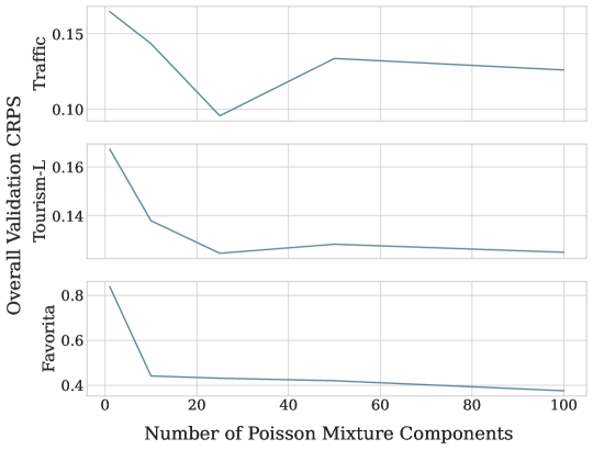
Figure 1: Poisson Mixture size ablation study. We found interesting bias-variance trade-offs controlled by the number of mixture components, both Traffic and Tourism-L have an optimal value of 25 components, beyond which the sCRPS validation performance worsens. We observed a classic U-shaped pattern. In the case of Favorita, the largest dataset, the validation sCRPS continued to improve through $K=100$.

For example, Figure 1 represents a simple hierarchy where each parent node is the sum of its children. Here the dimensions are $N_{a}=3$, $N_{b}=4$, and the hierarchical, aggregated and base series are respectively:

$$y_{\mathrm{Total},{\color[rgb]{0,0,0}{t}\color[rgb]{0,0,0}}}=y_{\beta_{1},{\color[rgb]{0,0,0}{t}\color[rgb]{0,0,0}}}+y_{\beta_{2},{\color[rgb]{0,0,0}{t}\color[rgb]{0,0,0}}}+y_{\beta_{3},{\color[rgb]{0,0,0}{t}\color[rgb]{0,0,0}}}+y_{\beta_{4},{\color[rgb]{0,0,0}{t}\color[rgb]{0,0,0}}}$$ (2)

$$\mathbf{y}_{[a],{\color[rgb]{0,0,0}{t}\color[rgb]{0,0,0}}}=\left[y_{\mathrm{Total},{\color[rgb]{0,0,0}{t}\color[rgb]{0,0,0}}},\;y_{\beta_{1},{\color[rgb]{0,0,0}{t}\color[rgb]{0,0,0}}}+y_{\beta_{2},{\color[rgb]{0,0,0}{t}\color[rgb]{0,0,0}}},\;y_{\beta_{3},{\color[rgb]{0,0,0}{t}\color[rgb]{0,0,0}}}+y_{\beta_{4},{\color[rgb]{0,0,0}{t}\color[rgb]{0,0,0}}}\right]^{\intercal}\qquad\mathbf{y}_{[b],{\color[rgb]{0,0,0}{t}\color[rgb]{0,0,0}}}=\left[y_{\beta_{1},{\color[rgb]{0,0,0}{t}\color[rgb]{0,0,0}}},\;y_{\beta_{2},{\color[rgb]{0,0,0}{t}\color[rgb]{0,0,0}}},\;y_{\beta_{3},{\color[rgb]{0,0,0}{t}\color[rgb]{0,0,0}}},\;y_{\beta_{4},{\color[rgb]{0,0,0}{t}\color[rgb]{0,0,0}}}\right]^{\intercal}$$

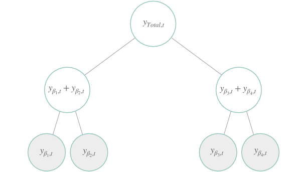
Figure 1: A simple three level time series hierarchical structure, with four bottom level variables. The disaggregated bottom variables are marked with gray background. In this description each node represents non overlapping series for a single point in time.

The constraint matrix of the Figure 1 example and the corresponding aggregations from Equation (2) is the following:

$${\color[rgb]{0,0,0}{\mathbf{S}_{[a,b][b]}}\color[rgb]{0,0,0}}=\begin{bmatrix}\\ {\color[rgb]{0,0,0}{\mathbf{A}_{\mathrm{[a][b]}}}\color[rgb]{0,0,0}}\\ \\ \\ \mathbf{I}_{\mathrm{[b][b]}}\\ \\ \end{bmatrix}=\begin{bmatrix}\;1&1&1&1\\ \;1&1&0&0\\ \;0&0&1&1\\ \hline\cr\;1&0&0&0\\ \;0&1&0&0\\ \;0&0&1&0\\ \;0&0&0&1\\ \end{bmatrix}$$

2.2 Mean Forecast Reconciliation Strategies

Given a forecast creation date $t$ and horizon $h$, the forecast indexes are denoted by $\tau\in[t+1:t+h]$. Most of the prior statistical solutions to the hierarchical forecasting challenge implement a two-stage process, first generating base forecasts $\hat{\mathbf{y}}_{[a,b],\tau}\in\mathbb{R}^{N_{a}+N_{b}}$, and then revising them into coherent forecasts $\tilde{\mathbf{y}}_{[a,b],\tau}$ through reconciliation. The reconciliation is compactly expressed by:

$$\tilde{\mathbf{y}}_{[a,b],\tau}={\color[rgb]{0,0,0}{\mathbf{S}_{[a,b][b]}}\color[rgb]{0,0,0}}\mathbf{P}_{[b][a,b]}\hat{\mathbf{y}}_{[a,b],\tau}$$ (3)

where ${\color[rgb]{0,0,0}{\mathbf{S}_{[a,b]}}\color[rgb]{0,0,0}}\in\mathbb{R}^{(N_{a}+N_{b})\times N_{b}}$ is the hierarchical aggregation matrix and $\mathbf{P}_{[b][a,b]}\in\mathbb{R}^{N_{b}\times(N_{a}+N_{b})}$ is a matrix determined by the reconciliation strategies. The most common reconciliation methods can be classified into top-down, bottom-up and alternative approaches.

• Bottom-Up: The simple bottom-up strategy, abbreviated as NaiveBU (Orcutt et al., 1968), first generates bottom level forecasts and then aggregates them to produce forecasts for all the series in the multivariate structure.

• Top-Down: The top-down strategy, abbreviated as TD (Gross & Sohl, 1990; Fliedner, 1999), distributes the total forecast, and then disaggregates it down the hierarchy using proportions that can be historical actuals or forecasted separately.

• Alternative: The more recent middle-out strategies, denoted as MO (Hyndman et al., 2011; Hyndman & Athanasopoulos, 2018)), treat the second stage reconciliation as an optimization problem for the matrix $\mathbf{P}_{[b][a,b]}$. These reconciliation techniques include among others Game-Theoretically OPtimal (GTOP; Van Erven & Cugliari (2015)), learning a projection for reducing quadratic loss, a generalized least squares model for minimizing trace of the squared error matrix, namely the minimum trace reconciliation (MinT; Wickramasuriya et al. (2019)) and the empirical risk minimization approach (ERM; Souhaib & Bonsoo (2019)).

Despite the advancements in alternative reconciliation strategies with statistical solutions, as mentioned in Section 1, there are still fundamental limitations. First, most post-process reconciliation methods produce mean forecasts but not probabilistic forecasts, with some exceptions that have relied on univariate statistical methods with strong probability assumptions for the base series that may be restrictive (Ben Taieb et al., 2017; Panagiotelis et al., 2020). Second, the mentioned methods independently learn the model parameters of the base level forecasts, limiting the base model’s optimization inputs to single series. This approach induces an over-fitting prone setting for complex nonlinear methods, which, as noted by the forecasting community, is one of their biggest challenges (Makridakis et al., 2018b). The implied data scarcity translates into a missed opportunity to leverage the flexibility of nonlinear methods.

2.3 Probabilistic Coherent Forecasting

There is a large body of related work on Bayesian hierarchical modeling of Spatio-temporal data; with joint coherent predictive distributions (Wikle et al., 1998; Diggle, 2013). These models, however, come with strong assumptions, as they typically assume a stationary Gaussian process to induce correlations and rely on Markov Chain Monte Carlo to estimate the posterior distribution (Diggle & Brix, 2001; Diggle, 2013). For modeling count data, variants of Bayesian Hierarchical Poisson Regression Models were introduced (Christiansen & Morris, 1997; Park & Lord, 2009), but they usually operate with linear model assumptions. There are few specialized methods on coherent probabilistic forecasting as most research on hierarchical forecasting has been limited to point predictions. Exceptions are the work by Shang & Hyndman (2017) and Jeon et al. (2019) that provide an early exploration of forecast quantile reconciliation; Ben Taieb et al. (2017) and Ben Taieb et al. (2021) that propose the combination of bottom-level forecast marginal distributions with empirical copula functions describing their dependencies to create aggregate predictive distributions. To the best of our knowledge, a formal definition of probabilistic coherence has only been explored by (Ben Taieb et al., 2021; Puwasala et al., 2018; Wickramasuriya, 2023; Panagiotelis et al., 2023). Ben Taieb et al. (2021) provides a convolution-based definition while Panagiotelis et al. (2023) provides a generalized and intuitive framework that we follow in our work and introduce below:

Definition 2.1.

(Probabilistic Coherence). Let $(\Omega_{[b]},\mathcal{F}_{[b]},\hat{\mathbb{P}}_{[b]})$ be a probabilistic forecast space, with sample space $\Omega_{[b]}$, $\mathcal{F}_{[b]}$ its $\sigma$-algebra, and $\hat{\mathbb{P}}_{[b]}$ a forecast probability. Let $\mathbf{S}_{[a,b][b]}(\cdot):\Omega_{[b]}\mapsto\Omega_{[a,b]}$ be the linear transformation implied by the constraints matrix. A coherent probabilistic forecast space $(\Omega_{[a,b]},\mathcal{F}_{[a,b]},\hat{\mathbb{P}}_{[a,b]})$ satisfies:

$$\hat{\mathbb{P}}_{[a,b]}\left(\mathbf{S}_{[a,b][b]}(\mathcal{B})\right)=\hat{\mathbb{P}}_{[b]}\left(\mathcal{B}\right)\quad\text{for any set }\mathcal{B}\in\mathcal{F}_{[b]}\text{ and {\color[rgb]{0,0,0}{set's image}\color[rgb]{0,0,0}} }\mathbf{S}_{[a,b][b]}(\mathcal{B})\in\mathcal{F}_{[a,b]}$$ (4)

i.e., it assigns a zero probability to sets in $\mathbb{R}^{N_{a}+N_{b}}$ not containing any coherent forecasts.

For a simple definition-satisfying example, consider three random variables ($Y_{\alpha},Y_{\beta_{1}},Y_{\beta_{2}}$) with $Y_{\alpha}{\color[rgb]{0,0,0}{:=}\color[rgb]{0,0,0}}Y_{\beta_{1}}+Y_{\beta_{2}}$. A coherent forecast assigns zero probability to the variable realizations $(y_{\alpha},\;y_{\beta_{1}},\;y_{\beta_{2}})$ if they do not satisfy the aggregation constraint $y_{\alpha}=y_{\beta_{1}}+y_{\beta_{2}}$. An equivalent definition of coherence is to require that the marginal distributions are derivable from the joint distribution of the bottom level random variables. In this case, the probability function of interest is $\hat{\mathbb{P}}(Y_{\beta_{1}},Y_{\beta_{2}})$, and the marginal probabilities can be derived from it using indicator functions as follows:

$$\hat{\mathbb{P}}(Y_{\beta_{1}}=y_{\beta_{1}})=\sum_{y_{\beta_{2}}}\hat{\mathbb{P}}(Y_{\beta_{1}}=y_{\beta_{1}},Y_{\beta_{2}}=y_{\beta_{2}})\quad\text{and}\quad\hat{\mathbb{P}}(Y_{\beta_{2}}=y_{\beta_{2}})=\sum_{y_{\beta_{1}}}\hat{\mathbb{P}}(Y_{\beta_{1}}=y_{\beta_{1}},Y_{\beta_{2}}=y_{\beta_{2}})$$

$$\hat{\mathbb{P}}(Y_{\alpha}=y_{\alpha})=\sum_{y_{\beta_{1}},y_{\beta_{2}}}\hat{\mathbb{P}}(Y_{\beta_{1}}=y_{\beta_{1}},Y_{\beta_{2}}=y_{\beta_{2}})\;\text{1}(y_{\alpha}=y_{\beta_{1}}+y_{\beta_{2}}){\color[rgb]{0,0,0}{,}\color[rgb]{0,0,0}}\quad\quad\quad\quad\;$$

where $\text{1}(y_{\alpha}=y_{\beta_{1}}+y_{\beta_{2}})$ equals 1 when $y_{\alpha}=y_{\beta_{1}}+y_{\beta_{2}}$, and 0 otherwise. The marginal probability for $Y_{\alpha}$, has the aggregation constraint built into its definition and is by construction a hierarchically coherent probability with respect to $\hat{\mathbb{P}}(Y_{\beta_{1}})$ and $\hat{\mathbb{P}}(Y_{\beta_{2}})$. Note that knowledge of the joint distribution is not required to generate hierarchically coherent forecast. However, if we had access to the joint distribution, constructing hierarchically coherent marginal distributions is straight forward.

2.4 Hierarchical Neural Forecasting

In the last decade, neural network-based forecasting methods have become ubiquitous in large-scale forecasting applications (Wen et al., 2017; Böse et al., 2017; Madeka et al., 2018; Eisenach et al., 2021), transcending industry boundaries into academia, as it has redefined the state-of-the-art in many practical tasks (Yu et al., 2018; Ravuri et al., 2021; Olivares et al., 2022) and forecasting competitions (Makridakis et al., 2018a, 2020).

The latest neural network-based solutions to the hierarchical forecasting challenge include methods like the Simultaneous Hierarchically Reconciled Quantile Regression (SHARQ; Han et al. (2021)) and Hierarchically Regularized Deep Forecasting (HIRED; Paria et al. (2021)) and the Probabilistic Robust Hierarchical Network (PROFHiT; Kamarthi et al. (2022)) that augment the training loss function with approximations to the hierarchical constraints. And Hierarchical End-to-End learning (HierE2E; Rangapuram et al. (2021)) that integrates an alternative reconciliation strategy in its forecasts through linear projections. With the exception of HierE2E, the rest of these methods encourage probabilistic coherence through regularization but do not guarantee it. Additionally, if a user requires updating the hierarchical structure of interest, a whole new optimization of the networks would be needed for the existing methods to forecast the structure correctly.

Our proposed method, DPMN, can address these deficiencies by specifying any network’s output as our proposed Poisson Mixture predictive distribution. With this predictive distribution, a model needs only to forecast the bottom-most level in the hierarchy, after which any desired hierarchical structure of interest can be predicted with guaranteed probabilistic hierarchical coherence.

3 Probabilistic Model

Figure 2: The Poisson Mixture distribution has desirable properties that make it well-suited for probabilistic hierarchical forecasting for count data. Under minimal conditions, its aggregation rule implies probabilistic coherence of the random variables it models.

3.1 Joint Poisson Mixture Distribution

In this work, we focus our attention on hierarchical forecasting of discrete events with non-negative variables. Many forecasting problems fall in this category as shown by the data sets described in Section 6. However, the general framework presented here works for continuous distributions as well with a suitably chosen base class for the mixture distribution, e.g., Gaussian distribution. For discrete events, we start by postulating that the forecast joint probability of the bottom level future multivariate time series’ realization $\mathbf{y}_{[b][t+1:t+h]}\in\mathbb{N}^{N_{b}\times h}$ is:

$$\begin{split}\hat{\mathbb{P}}\left(\mathbf{y}_{[b][t+1:t+{\color[rgb]{0,0,0}{h}\color[rgb]{0,0,0}}]}|\;\boldsymbol{\lambda}_{[b][k][t+1:t+h]}\right)&=\sum_{{\color[rgb]{0,0,0}{\kappa}\color[rgb]{0,0,0}}=1}^{{\color[rgb]{0,0,0}{N_{k}}\color[rgb]{0,0,0}}}w_{\color[rgb]{0,0,0}{\kappa}\color[rgb]{0,0,0}}\prod_{(\beta,\tau)\in[b][t+1:t+h]}\mathrm{Poisson}\left(y_{{\color[rgb]{0,0,0}{\beta}\color[rgb]{0,0,0}},{\color[rgb]{0,0,0}{\tau}\color[rgb]{0,0,0}}}|\lambda_{{\color[rgb]{0,0,0}{\beta}\color[rgb]{0,0,0}},{\color[rgb]{0,0,0}{\kappa}\color[rgb]{0,0,0}},{\color[rgb]{0,0,0}{\tau}\color[rgb]{0,0,0}}}\right)\\ &=\sum_{{\color[rgb]{0,0,0}{\kappa}\color[rgb]{0,0,0}}=1}^{{\color[rgb]{0,0,0}{N_{k}}\color[rgb]{0,0,0}}}w_{\color[rgb]{0,0,0}{\kappa}\color[rgb]{0,0,0}}\prod_{(\beta,\tau)\in[b][t+1:t+h]}\frac{\lambda_{\beta,{\color[rgb]{0,0,0}{\kappa}\color[rgb]{0,0,0}},\tau}^{y_{\beta,\tau}}}{y_{\beta,\tau}!}e^{-\lambda_{\beta,{\color[rgb]{0,0,0}{\kappa}\color[rgb]{0,0,0}},\tau}}\end{split}$$ (5)

The mixture model describes individual bottom level time series and their correlations through the distribution of the mixture’s latent variables defined by the Poisson rates $\boldsymbol{\lambda}_{[b][k][t+1:t+h]}\in\mathbb{R}^{N_{b}\times N_{k}\times h}$ and the associated weights $\mathbf{w}_{[k]}\in[0,1]^{N_{k}}$, with $\mathbf{w}_{[k]}\geq 0$ and $\sum_{\kappa=1}^{N_{k}}w_{\kappa}=1$. The number of Poisson components $\mid[k]\mid=N_{k}$ is a hyperparameter of the model that controls the flexibility of the mixture distribution. The mixture distribution can also be interpreted as a multivariate kernel density approximation, with Poisson kernels, to the actual joint probability distribution $\mathbb{P}\left(\mathbf{y}_{[b][t+1:t+{\color[rgb]{0,0,0}{h}\color[rgb]{0,0,0}}]}\right)$. We show an example of the Poisson mixture distribution in Figure 2.

The joint distribution in Equation (5), assumes that the modeled observations $\mathbf{y}_{[b][t+1:t+h]}$ are conditionally independent given the latent Poisson rates $\boldsymbol{\lambda}_{[b][k][t+1:t+h]}$. That is for all bottom level series and horizons $(\beta,\tau)\neq(\beta^{\prime},\tau^{\prime})\text{, }(\beta,\tau),(\beta^{\prime},\tau^{\prime})\in[b][t+1:t+h]$ and $\kappa\in[k]$:

$$\hat{\mathbb{P}}(Y_{\beta,\tau},Y_{\beta^{\prime},\tau^{\prime}}|\lambda_{\beta,{\color[rgb]{0,0,0}{\kappa}\color[rgb]{0,0,0}},\tau},\lambda_{\beta^{\prime},{\color[rgb]{0,0,0}{\kappa}\color[rgb]{0,0,0}},\tau^{\prime}})=\hat{\mathbb{P}}(Y_{\beta,\tau}|\lambda_{\beta,{\color[rgb]{0,0,0}{\kappa}\color[rgb]{0,0,0}},\tau})\hat{\mathbb{P}}(Y_{\beta^{\prime},\tau^{\prime}},|\lambda_{\beta^{\prime},{\color[rgb]{0,0,0}{\kappa}\color[rgb]{0,0,0}},\tau^{\prime}})$$ (6)

3.2 Marginal Distributions for Bottom Series

Equation (5) describes the joint distribution of all bottom level time series. We can derive the marginal distribution for one of the bottom level series $\beta\in[b]$ and for a single future time period $\tau\in[t+1:t+h]$ by integrating out the remaining series and time indices. The marginal distribution is:

$$\hat{\mathbb{P}}(Y_{\beta,\tau}=y_{\beta,\tau}) =\sum_{\mathbf{y}_{[b][t+1:t+h]\setminus(\beta,\tau)}}\sum_{\kappa=1}^{N_{k}}w_{\kappa}\prod_{(\beta^{\prime},\tau^{\prime})\in[b][t+1:t+h]}\mathrm{Poisson}(y_{\beta^{\prime},\tau^{\prime}}|\lambda_{\beta^{\prime},\kappa,\tau^{\prime}})$$

$$=\sum_{\kappa=1}^{N_{k}}w_{\kappa}\;\mathrm{Poisson}(y_{\beta,\tau}|\lambda_{\beta,\kappa,\tau})\times\prod_{(\beta^{\prime},\tau^{\prime})\in[b][t+1:t+h]\setminus(\beta,\tau)}\quad\sum_{y_{\beta^{\prime},\tau^{\prime}}}\mathrm{Poisson}(y_{\beta^{\prime},\tau^{\prime}}|\lambda_{\beta^{\prime},\kappa,\tau^{\prime}})$$

$$=\sum_{\kappa=1}^{N_{k}}w_{\kappa}\;\mathrm{Poisson}(y_{\beta,\tau}|\lambda_{\beta,\kappa,\tau})$$ (7)

We get a clean final expression for the marginal distribution, which is equivalent to simply dropping all other time series and time periods from the product in Equation (5).

3.3 Marginal Distributions for Aggregate Series

An important consequence of the conditional independence in Equation (6) is that the marginal distributions at aggregate levels $\mathbf{y}_{[a],\tau}$ can be computed via simple component-wise addition of the lower level Poisson rates. For example consider an aggregate level variable $Y_{\alpha,\tau}{\color[rgb]{0,0,0}{:=}\color[rgb]{0,0,0}}Y_{\beta_{1},\tau}+Y_{\beta_{2},\tau}$. The marginal distribution for $Y_{\alpha,\tau}$ can be derived from the joint distribution in Equation (5) as follows. First marginalize all other series and time indices (as done in Section 3.2 above), which gives us the joint distribution for $Y_{\beta_{1},\tau}$ and $Y_{\beta_{2},\tau}$

$$\hat{\mathbb{P}}(Y_{\beta_{1},\tau}=y_{\beta_{1},\tau},Y_{\beta_{2},\tau}=y_{\beta_{2},\tau})=\sum_{\kappa=1}^{N_{k}}w_{\kappa}\;\mathrm{Poisson}(y_{\beta_{1},\tau}|\lambda_{\beta_{1},\kappa,\tau})\times\mathrm{Poisson}(y_{\beta_{2},\tau}|\lambda_{\beta_{2},\kappa,\tau})$$

Now, the aggregate marginal distribution is

$$\hat{\mathbb{P}}(Y_{\alpha,\tau}=y_{\alpha,\tau}) = \sum_{y_{\beta_{1},\tau},y_{\beta_{2},\tau}}\hat{\mathbb{P}}(Y_{\beta_{1},\tau}=y_{\beta_{1},\tau},Y_{\beta_{2},\tau}=y_{\beta_{2},\tau})\;\text{1}(y_{a,\tau}=y_{\beta_{1},\tau}+y_{\beta_{2},\tau})$$

For each mixture component with index $\kappa$, the distributions of $y_{\beta_{1},\tau}$ and $y_{\beta_{2},\tau}$ conditioned on respective Poisson rates $\lambda_{\beta_{1},\kappa,\tau}$ and $\lambda_{\beta_{2},\kappa,\tau}$ are independent Poisson distributions, and therefore, the distribution of the aggregate is another Poisson Mixture with parameters $\lambda_{{\color[rgb]{0,0,0}{\alpha}\color[rgb]{0,0,0}},\kappa,\tau}=\lambda_{\beta_{1},\kappa,\tau}+\lambda_{\beta_{2},\kappa,\tau}$.

$$\hat{\mathbb{P}}({\color[rgb]{0,0,0}{Y_{\alpha,\tau}=}\color[rgb]{0,0,0}}y_{\alpha,\tau})=\sum_{\kappa=1}^{N_{k}}w_{\kappa}\mathrm{Poisson}(y_{{\color[rgb]{0,0,0}{\alpha}\color[rgb]{0,0,0}},\tau}|\lambda_{{\color[rgb]{0,0,0}{\alpha}\color[rgb]{0,0,0}},\kappa,\tau}=\lambda_{\beta_{1},\kappa,\tau}+\lambda_{\beta_{2},\kappa,\tau})$$ (8)

The aggregation rule can be concisely described as:

$$\boldsymbol{\lambda}_{[a][k],\tau}=\mathbf{A}_{\mathrm{[a][b]}}\boldsymbol{\lambda}_{[b][k],\tau}$$ (9)

with $\mathbf{A}_{\mathrm{[a][b]}}$ the hierarchical aggregation matrix defined in Section 2.1. The joint predictive distribution is hierarchically coherent by construction. We offer a formal proof of DPMN’s satisfaction of the probabilistic coherence property from Definition 2.1 in A.

3.4 Covariance Matrix

Using the law of total covariance and the conditional independence from Equation (6), we show in B that the covariance of any two bottom level series naturally follows:

$$\mathrm{Cov}(Y_{\beta,\tau},Y_{\beta^{\prime},\tau^{\prime}})=\overline{\lambda}_{\beta,\tau}{\color[rgb]{0,0,0}{\text{1}(\beta=\beta^{\prime})\text{1}(\tau=\tau^{\prime})}\color[rgb]{0,0,0}}+\sum_{\kappa=1}^{N_{k}}w_{\kappa}\left(\lambda_{\beta,\kappa,\tau}-\overline{\lambda}_{\beta,\tau}\right)\left(\lambda_{\beta^{\prime},\kappa,\tau^{\prime}}-\overline{\lambda}_{\beta^{\prime},\tau^{\prime}}\right)$$ (10)

where $\overline{\lambda}_{\beta,\tau}=\sum_{\kappa=1}^{N_{k}}w_{\kappa}\lambda_{\beta,\kappa,\tau}$ . C shows the non-diagonal covariance matrix expressivity, as determined by its rank, depends on the number of mixture components from Equation (5).

4 Parameter Estimation and Inference

4.1 Maximum Joint Likelihood

To estimate model parameters, we can maximize the joint likelihood implied by the joint distribution from Equation (5). Let $\boldsymbol{\theta}$ represent the neural network parameters as described in Section 5, we parameterize the probabilistic model with Poisson rates $\boldsymbol{\lambda}_{[b][k][t+1:t+h]}$ as follows:

$$\boldsymbol{\lambda}_{[b][k][t+1:t+h]} :=\hat{\boldsymbol{\lambda}}_{[b][k][t+1:t+h]}{\color[rgb]{0,0,0}{(\boldsymbol{\theta})}\color[rgb]{0,0,0}}$$ (11)

$$\mathbf{w}_{[k]} :=\hat{\mathbf{w}}_{[k]}{\color[rgb]{0,0,0}{(\boldsymbol{\theta})}\color[rgb]{0,0,0}}$$

The Poisson rates and the mixture weights are conditioned through the network’s parameters on forecasting features discussed in Section 5.1. The negative log-likelihood can then be written:

$$\mathcal{L}(\boldsymbol{\theta})=-\mathrm{log}\left[\sum_{\kappa=1}^{N_{k}}\hat{w}_{\kappa}(\boldsymbol{\theta})\prod_{(\beta,\tau)\in[b][t+1:t+h]}\left(\frac{(\hat{\lambda}_{\beta,\kappa,\tau}(\boldsymbol{\theta}))^{{}^{y_{\beta,\tau}}}\exp{\{-\hat{\lambda}_{\beta,\kappa,\tau}(\boldsymbol{\theta})\}}}{(y_{\beta,\tau})!}\right)\right]$$ (12)

This is the same expression as the multivariate probability mass function in Equation (5) but parametrized as a function of the neural network parameters $\theta$. The maximum likelihood estimation method (MLE) has desirable properties like statistical efficiency and consistency. However, the mixture components cannot be estimated separately, and for this reason, MLE is only feasible for hierarchical time series with a small number of series. Additional exploration is needed to make the estimation scalable.

4.2 Maximum Composite Likelihood

A computationally efficient alternative to MLE for estimating the model parameters is to maximize the composite likelihood. This method involves breaking up the high-dimensional space into smaller sub-spaces, and the composite likelihood consists of the weighted product of the marginal likelihoods of the subspaces (Lindsay, 1988). For simplicity, we used uniform weights.

In addition to the computational efficiency, maximizing the composite likelihood provides a robust and unbiased estimate of marginal model parameters with the drawback that the model inference may suffer from properties similar to a misspecified model (Varin et al., 2011). We will discuss variants of the composite likelihood below.

4.2.1 Naive Bottom Up

A simple option of using composite likelihood is to define each bottom-level time series as its likelihood sub-space and treat them as independent during model training  (Orcutt et al., 1968). We refer to this estimation method for the DPMN as Naive Bottom Up (DPMN-NaiveBU). The negative logarithm of the DPMN-NaiveBU composite likelihood is:

$$\mathcal{L}_{\mathrm{NaiveBU}}(\boldsymbol{\theta})=-\sum_{\beta\in[b]}\mathrm{log}\left[\sum_{\kappa=1}^{N_{k}}\hat{w}_{\kappa}(\boldsymbol{\theta})\prod_{\tau\in[t+1:t+h]}\left(\frac{(\hat{\lambda}_{\beta,\kappa,\tau}(\boldsymbol{\theta}))^{{}^{y_{\beta,\tau}}}\exp{\{-\hat{\lambda}_{\beta,\kappa,\tau}(\boldsymbol{\theta})\}}}{(y_{\beta,\tau})!}\right)\right]$$ (13)

Even though the sub-space consists of single bottom level time series, DPMN-NaiveBU is still a multi-variate model with the composite likelihood defined over multiple time points $[t+1:t+h]$. Maximizing the DPMN-NaiveBU composite likelihood will still learn correlations across the time points and will generate coherent forecast distributions for aggregations in the time dimension. It does not attempt, however, to discover correlations across different time series.

4.2.2 Group Bottom Up

If prior information helps us identify groups of time series with interesting correlation structures, we may estimate them by including the groups in the composite likelihood. We refer to this estimation method for the DPMN as Group Bottom Up (DPMN-GroupBU). Let $\mathcal{G}=\{[g_{i}]\}$ be time-series groups, then the negative log composite likelihood for the DPMN-GroupBU is

$$\mathcal{L}_{\mathrm{GroupBU}}(\boldsymbol{\theta})=-\sum_{[g_{i}]\in\mathcal{G}}\mathrm{log}\left[\sum_{\kappa=1}^{N_{k}}\hat{w}_{\kappa}(\boldsymbol{\theta})\prod_{(\beta,\tau)\in[g_{i}][t+1:t+h]}\left(\frac{(\hat{\lambda}_{\beta,\kappa,\tau}(\boldsymbol{\theta}))^{{}^{y_{\beta,\tau}}}\exp{\{-\hat{\lambda}_{\beta,\kappa,\tau}(\boldsymbol{\theta})\}}}{(y_{\beta,\tau})!}\right)\right]$$ (14)

The main advantage over DPMN-NaiveBU is that the model now learns cross-series relationships. In this paper we only rely on intuitive grouping like geographic proximity, but one could in principle employ more sophisticated methods like clustering to define the groups. To optimize the learning objective we use stochastic gradient descent, and sample train series batches at the group level.

4.3 Forecast Inference

As mentioned earlier, model inference from composite likelihood estimation suffers from problems similar to model misspecification. This is because of the independence assumed across sub-spaces. In our model, the maximum composite likelihood estimates do not understand how mixture components learnt for one sub-space relate to mixture components learnt for a different subspace. However, we need to identify mixture components across sub-spaces in order to define the joint distribution in Equation (5) across all bottom level time series. Knowing this joint distribution is at the crux of forecast inference from our model. Fortunately, there is a natural way for us to resolve this issue. Both in the DPMN-NaiveBU composite likelihood in Equation (13) and in the DPMN-GroupBU composite likelihood in Equation (14), the weights $\hat{\mathbf{w}}_{[k]}(\theta)\in\mathbb{R}^{N_{k}}$ are shared across all sub-spaces. We identify components with the same weight as belonging to the same multivariate sample, and hence providing the full joint distribution. We call this method weight matching.

For the DPMN-NaiveBU estimation, the weight matching method is a strong statistical assumption, extrapolating from independent marginal distributions of each series to the full joint distribution. The DPMN-GroupBU approach significantly alleviates this problem because the model parameters are well defined within each group $[g_{i}]\in\mathcal{G}$ and if most of the interesting correlations are already captured within each group, then much less burden is placed on the weight matching method. We show in the evaluation of Section 6 that both DPMN-NaiveBU and DPMN-GroupBU models perform favorably when compared to other mean and probabilistic hierarchical forecasting methods, and between the two, DPMN-GroupBU is generally more accurate when the time series grouping given is informative.

5 Deep Poisson Mixture Network

Our primary goal is to create a probabilistic coherent forecasting model that is accurate and efficient. For this purpose, we opt to extend the MQ-Forecaster family (Wen et al., 2017; Eisenach et al., 2021), proven by its history of industry service, with the Poisson mixture distribution. We refer to this model as the Deep Poisson Mixture Network (DPMN). Our MQ-Forecaster architecture selection is driven by its high computational efficiency, consequence of the forking-sequences technique and multi-step forecasting strategy, in addition to its ability to incorporate static and known future temporal features.

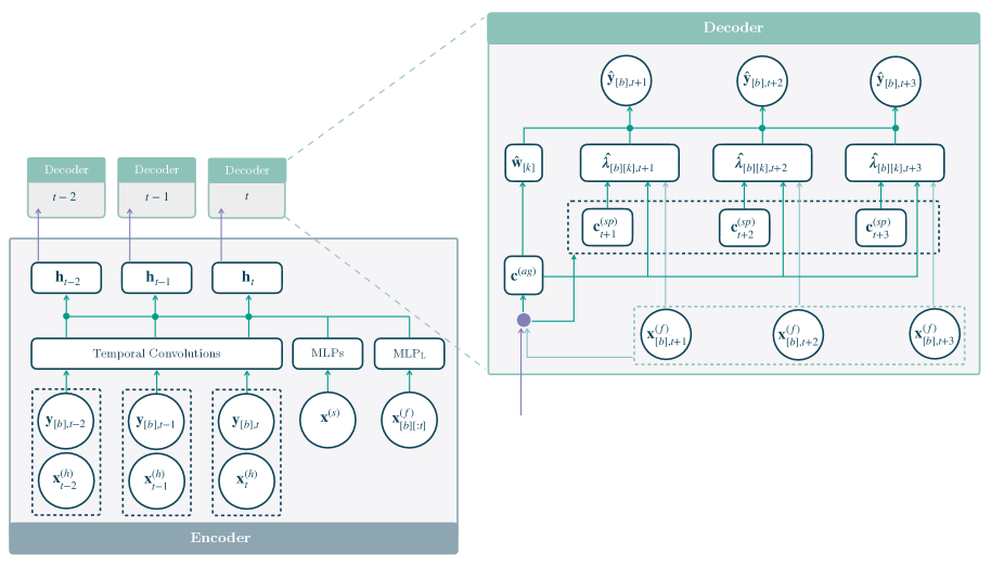
Figure 3: The Deep Poisson Mixture Network (DPMN) is a Sequence-to-Sequence with Context network that uses dilated temporal convolutions as the primary encoder and multilayer perceptron based decoders for a direct multi-step forecast. The forked decoders share their parameters and create the multivariate forecast distribution for each time point in the encoder, making the architecture efficient in its optimization and predictions.

5.1 Model Features

As part of the innovations within our work, we propose to separate the bottom-level and aggregate-level features that we use in the forecasts. Sharing aggregate-level features across their respective bottom series simplifies the model’s inputs and reduces redundant information, while greatly improving the model’s memory usage efficiency.

We follow the hierarchical forecasting literature practice for the static features and use group identifiers implied by the hierarchy structure. We denote the static features, composed of features shared across the bottom series $\tilde{\mathbf{x}}^{(s)}$ and bottom level-specific features $\mathbf{x}_{[b]}^{(s)}$ by:

$$\mathbf{x}^{(s)}=\{\mathbf{x}^{(s)}_{[b]},\;\,\tilde{\mathbf{x}}^{(s)}\}.$$ (15)

Regarding temporal features, for the bottom level, we use the bottom series’ past; for the aggregate level we use the parent node series’ past. The future temporal information available can be task specific inputs like prices or promotions in the context of product demand forecasting, or other simpler model forecasts as inputs, such as Naive1 or SeasonalNaive that help the model predict series levels and seasonalities. Similarly to the static features, we also distinguish the temporal shared features $\tilde{\mathbf{x}}^{(h)}_{[:{\color[rgb]{0,0,0}{t}\color[rgb]{0,0,0}}]},\tilde{\mathbf{x}}^{(f)}_{[:{\color[rgb]{0,0,0}{t+h}\color[rgb]{0,0,0}}]}$ and the temporal bottom level-specific features $\mathbf{x}^{(h)}_{[b][t]},\mathbf{x}^{(f)}_{[b][:t+h]}$. With this consideration, we denote the historical and future temporal features by:

$$\mathbf{x}^{(h)}_{[:{\color[rgb]{0,0,0}{t}\color[rgb]{0,0,0}}]}=\{\mathbf{x}^{(h)}_{[b][:{\color[rgb]{0,0,0}{t}\color[rgb]{0,0,0}}]},\;\,\tilde{\mathbf{x}}^{(h)}_{[:{\color[rgb]{0,0,0}{t}\color[rgb]{0,0,0}}]}\}\qquad\text{and}\qquad\mathbf{x}^{(f)}_{[:{\color[rgb]{0,0,0}{t+h}\color[rgb]{0,0,0}}]}=\{\mathbf{x}^{(f)}_{[b][:{\color[rgb]{0,0,0}{t+h}\color[rgb]{0,0,0}}]},\;\,\tilde{\mathbf{x}}^{(f)}_{[:{\color[rgb]{0,0,0}{t+h]}\color[rgb]{0,0,0}}}\}$$ (16)

5.2 Model Architecture

In summary, the DPMN builds on the MQ-Forecaster architecture that is based on Sequence-to-Sequence with Context network (Seq2SeqC; Cho et al. (2014)). The DPMN uses dilated temporal convolutions (TempConv; van den Oord et al. (2016)) to encode the available history into hidden states and uses forked decoders based on Multi-Layer Perceptron (MLP; Rosenblatt (1961)) in a direct multi-horizon forecast strategy (Amir & Souhaib, 2016). We describe below in further detail the components of the model. Other hyperparameter details are available in Table A5.

5.2.1 Encoder

As explained earlier the DPMN main encoder is a stack of dilated temporal convolutions. Additionally, we use a global dense layer to encode the static features and a local dense layer, shared across time, to encode the available future information. The encoder for each time ${\color[rgb]{0,0,0}{t}\color[rgb]{0,0,0}}$ and its components are described in Equation (LABEL:equation:encoders).

$$\mathbf{h}^{(h)}_{{\color[rgb]{0,0,0}{t}\color[rgb]{0,0,0}}} =\{\mathbf{h}_{1,{\color[rgb]{0,0,0}{t}\color[rgb]{0,0,0}}}^{(h)}\,,\,\mathbf{h}_{2,{\color[rgb]{0,0,0}{t}\color[rgb]{0,0,0}}}^{(h)}\}=\{\mathbf{TempConv}(\mathbf{x}^{(h)}_{[b][:{\color[rgb]{0,0,0}{t}\color[rgb]{0,0,0}}]})\;,\;\mathbf{TempConv}(\tilde{\mathbf{x}}^{(h)}_{[:{\color[rgb]{0,0,0}{t}\color[rgb]{0,0,0}}]})\}$$ (17)

$$\mathbf{h}^{(s)} =\{\mathbf{h}_{1}^{(s)}\,,\,\mathbf{h}_{2}^{(s)}\}=\{\mathbf{MLP}(\mathbf{x}^{(s)}_{[b]})\;,\;\mathbf{MLP}(\tilde{\mathbf{x}}^{(s)})\}$$

$$\mathbf{h}^{(f)}_{{\color[rgb]{0,0,0}{t}\color[rgb]{0,0,0}}} =\mathbf{MLP}_{L}(\mathbf{x}^{(f)}_{[b][:{\color[rgb]{0,0,0}{t}\color[rgb]{0,0,0}}+h]})$$

The encoder’s output in Equation (LABEL:equation:encoders2) is a set of shared and bottom level encoded features $\mathbf{h}_{1,{\color[rgb]{0,0,0}{t}\color[rgb]{0,0,0}}}$ and $\mathbf{h}_{2,{\color[rgb]{0,0,0}{t}\color[rgb]{0,0,0}}}$. The first concatenates all the encoded past $\mathbf{h}^{(h)}_{1,{\color[rgb]{0,0,0}{t}\color[rgb]{0,0,0}}},\,\mathbf{h}^{(h)}_{2,{\color[rgb]{0,0,0}{t}\color[rgb]{0,0,0}}}\in\mathbb{R}^{N_{cf}}$, static $\mathbf{h}^{(s)}_{1},\,\mathbf{h}^{(s)}_{2}\in\mathbb{R}^{N_{s}}$ and available future $\mathbf{h}^{(f)}_{{\color[rgb]{0,0,0}{t}\color[rgb]{0,0,0}}}\in\mathbb{R}^{N_{f}}$ information. The second one concatenates the encoded past $\mathbf{h}^{(h)}_{2,{\color[rgb]{0,0,0}{t}\color[rgb]{0,0,0}}}\in\mathbb{R}^{N_{cf}}$ and static $\mathbf{h}^{(s)}_{2}\in\mathbb{R}^{{N}_{s}}$ shared features.

$$\mathbf{h}_{{\color[rgb]{0,0,0}{t}\color[rgb]{0,0,0}}} =\{\mathbf{h}_{1,{\color[rgb]{0,0,0}{t}\color[rgb]{0,0,0}}},\;\mathbf{h}_{2,{\color[rgb]{0,0,0}{t}\color[rgb]{0,0,0}}}\}=\{[\mathbf{h}^{(h)}_{1,{\color[rgb]{0,0,0}{t}\color[rgb]{0,0,0}}}|\mathbf{h}^{(h)}_{2,{\color[rgb]{0,0,0}{t}\color[rgb]{0,0,0}}}|\mathbf{h}^{(s)}_{1}|\mathbf{h}^{(s)}_{2}|\mathbf{h}^{(f)}_{{\color[rgb]{0,0,0}{t}\color[rgb]{0,0,0}}}],\;\;\,[\mathbf{h}^{(h)}_{2,{\color[rgb]{0,0,0}{t}\color[rgb]{0,0,0}}}|\mathbf{h}^{(s)}_{2}]\}$$ (18)

5.2.2 Forked Decoders

The DPMN uses a two-branch MLP decoder. The first decoder branch, summarizes the encoder output and future available information into two contexts: The horizon-agnostic context set $\mathbf{c}^{(ag)}\in\mathbb{R}^{N_{ag}}$ and the horizon-specific context $\mathbf{c}^{(sp)}_{[{\color[rgb]{0,0,0}{t}\color[rgb]{0,0,0}}+1:{\color[rgb]{0,0,0}{t}\color[rgb]{0,0,0}}+h]}\in\mathbb{R}^{N_{sp}\times h}$ that provides structural awareness of the forecast horizon and plays a crucial role in expressing recurring patterns in the time series if any. Equation (LABEL:equation:forked_decoders1) describes the first decoder branch:

$$\mathbf{c}^{(ag)}=\{\mathbf{c}^{(ag)}_{1},\,\mathbf{c}^{(ag)}_{2}\}=\{\mathbf{MLP}(h_{1,{\color[rgb]{0,0,0}{t}\color[rgb]{0,0,0}}}),\,\mathbf{MLP}(\mathbf{h}_{2,{\color[rgb]{0,0,0}{t}\color[rgb]{0,0,0}}})\}$$ (19)

$$\mathbf{c}^{(sp)}_{[{\color[rgb]{0,0,0}{t}\color[rgb]{0,0,0}}+1:{\color[rgb]{0,0,0}{t}\color[rgb]{0,0,0}}+h]}=\mathbf{MLP}_{L}(\mathbf{h}_{1,{\color[rgb]{0,0,0}{t}\color[rgb]{0,0,0}}})$$

The second decoder branch adapts the horizon-specific and horizon-agnostic contexts into the parameters of the Poisson mixture distribution. For the horizon-specific Poisson rates, we use the forking-sequence technique with a series of decoders with shared parameters for each time point in $[t+1:t+h]$ and for the mixture weights, we apply an MLP followed by a softmax on the aggregate horizon agnostic context. Equation (20) describes the second decoder branch:

$$\hat{\boldsymbol{\lambda}}_{[b][k][t+1:t+h]} =\mathbf{MLP}_{L}(\mathbf{c}^{(ag)}_{1},\,\mathbf{c}^{(sp)}_{[{\color[rgb]{0,0,0}{t}\color[rgb]{0,0,0}}+1:{\color[rgb]{0,0,0}{t}\color[rgb]{0,0,0}}+h]},\,\mathbf{x}^{(f)}_{[b][{\color[rgb]{0,0,0}{t}\color[rgb]{0,0,0}}+1:{\color[rgb]{0,0,0}{t}\color[rgb]{0,0,0}}+h]})$$ (20)

$$\hat{\mathbf{w}}_{[k]} =\mathrm{SoftMax}(\mathbf{MLP}(\mathbf{c}^{(ag)}_{2}))$$

6 Empirical Evaluation

6.1 Hierarchical Forecasting Datasets

To evaluate our method, we consider three forecasting tasks where the objective is to provide quantile forecasts for each time series in the group or hierarchy structure. All the three datasets that we use in the empirical evaluation  are publicly available and have been used in the hierarchical forecasting literature (Wickramasuriya et al., 2019; Souhaib & Bonsoo, 2019; Rangapuram et al., 2021; Paria et al., 2021). Table 1 summarizes the datasets’ characteristics.

Table 1: Summary, hierarchical structure and forecast horizon of datasets used in our empirical study.

Dataset	Total	Aggregated	Bottom	Levels	Observations	Horizon ($h$)
Traffic	207	7	200	4	366	1
Tourism-L	555	175	$76\,/\,304$	$4\,/\,5$	228	12
Favorita	371,312	153,386	217,944	4	1,688	34

(a) Traffic

(b) Tourism

(c) Favorita

Figure 4: Visualization of the hierarchical constraints of the empirical evaluation datasets. (a) Traffic groups 200 highways’ occupancy series into quarters, halves and total. (b) Tourism-L groups its 555 regional visit series, into a combination of travel purpose, zones, states and country geographical aggregations. (c) Favorita groups its grocery sales geographically, by store, city, state, and country levels.

The Tourism-L (Tourism Australia, Canberra, 2019) is an Australian Tourism dataset that contains 555 monthly visit series from 1998 to 2016, grouped by geographical regions and travel purposes. Favorita (Corporación Favorita, 2018) is a Kaggle competition dataset of grocery item sales daily history with additional information on promotions, items, stores, and holidays, containing 371,312 series from January 2013 to August 2017, with a geographic hierarchy of states, cities, and stores. We show their hierarchical constraints matrix in Figure 4. Traffic (Dua & Graff, 2017; Souhaib & Bonsoo, 2019) measures the occupancy of 200 car lanes in the San Francisco Bay Area, randomly grouped into a year of daily observations with 207 series hierarchical structure.

The datasets provide an opportunity to showcase the broad applicability of the DPMN, as each has unique characteristics. Tourism-L allows us to test the DPMN to model group structures with multiple hierarchies. Favorita allows us to test the DPMN on a large-scale dataset. Traffic  is composed of randomly assigned hierarchical groupings that may not have any informative structures for the DPMN to learn with GroupBU. Finally, Favorita contains some non-count demand values (grocery produce sold by weight) and Traffic aggregated occupancy rates are non-count data, so modeling these datasets with a Poisson mixture limits the maximum accuracy we can achieve.

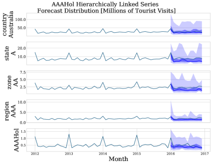
(a) DPMN-NaiveBU

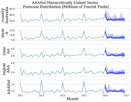
(b) DPMN-GroupBU

Figure 5: DPMN-NaiveBU and DPMN-GroupBU forecast distributions on a Tourism-L hierarchically linked time series. The top row shows total tourist visits in Australia, the second row shows the visits to Australia for the North South Wales state (A), the third row shows the holiday visits in the metropolitan Area of New South Wales (AA), the fourth row shows the Sidney total visits (AAA), the final row shows the holiday visits to Sidney. Forecast distributions, 99% and 75% prediction intervals in light and dark blue.

6.2 Time Series Covariance Modeling

We present in this subsection an illustrative example demonstrating how DPMN leverages the flexibility and expressiveness of the multivariate Poisson mixture distribution to capture interesting correlations present in hierarchical time series datasets to improve forecast sharpness. Figure 5 shows a comparison of forecasts generated by the DPMN-NaiveBU and the DPMN-GroupBU methods at various aggregation levels of the Tourism-L dataset. The DPMN-GroupBU method accurately estimates correlations in bottom-level series, improving the forecast distribution concentration of the upper-level series. In contrast, the DPMN-NaiveBU method performs well on disaggregated series and mean forecasts, but suffers from significant model misspecification which reduces the sharpness of forecasts at the aggregated levels. We find that the DPMN-GroupBU generally does better when informative group series structure is present in the data, like in Tourism-L and Favorita datasets. DPMN-NaiveBU produces comparable results at disaggregated levels of all datasets and outperforms hierarchical forecasting baselines when hierarchical structure is noisy or not informative, as in the Traffic dataset. Our intuitions are validated by the empirical results presented in Section 6.6.

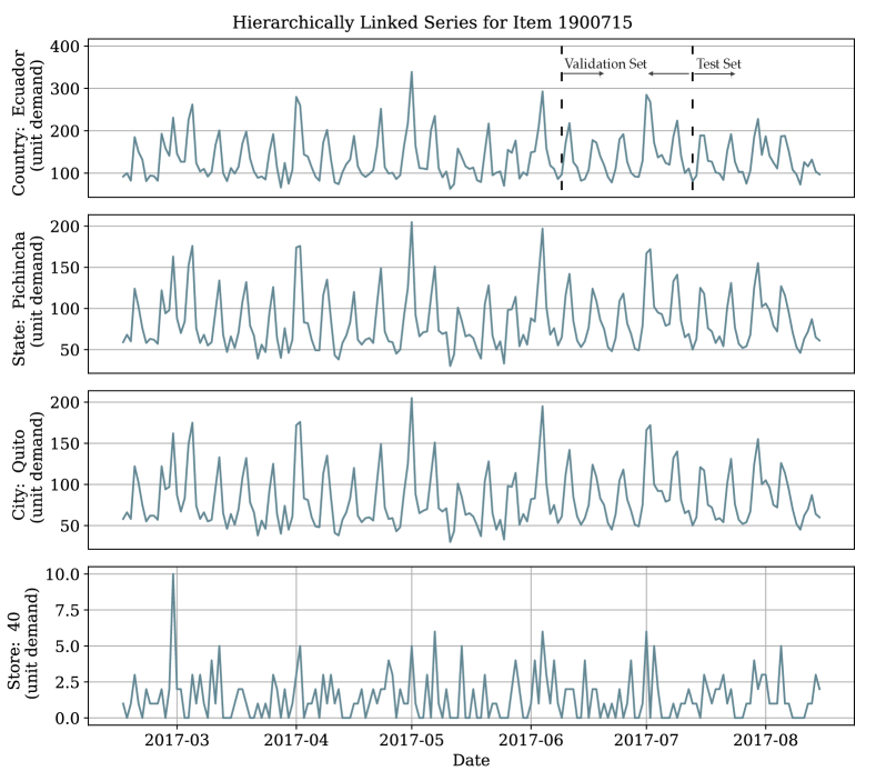
Figure 6: Example of a Favorita geographically linked time series. The top level shows the sales for a grocery item in the country of Ecuador. The second level shows the sold units within Pichincha state, the third level shows the sales for Quito city, the final level shows Store 40 item sales. For this dataset, the training set comprises all the observations preceding the validation and test sets. The validation set (between the first and second dotted lines) is the 34 days before the test set. The held-out test set (marked by the last dotted line) is the last 34 observations.

6.3 Datasets Partition and Preprocessing

For the main experiments we separate the train, validation and test datasets’ partition as follows: we hold out the final horizon-length observations as the test set. In a sliding-window fashion, we use the horizon-length that precedes the test set as the validation set and treat the rest of the past information as the training set. A partition example is depicted in Figure 6.

For comparability purposes with the most recent hierarchical forecasting literature, we keep ourselves as close as possible to the preprocessing and wrangling of the datasets to that of Rangapuram et al. (2021). In general, the static variables that we consider on all the datasets correspond to the hierarchical and group designators as categorical variables implied by the hierarchical constraint matrix. The temporal covariates that we consider are the time series for the upper levels of the hierarchy, as well as calendar covariates associated with the time series frequency of each dataset. As future data, we include calendar covariates to help the DPMN capture seasonalities.

Table 2: Considered hyperparameters for the Deep Poisson Mixture Network (DPMN). The learning rate, random seed, and SGD epochs that performed best on the validation set were selected automatically in each HYPEROPT run. The remaining model parameters were configured once per dataset, as explained in F.
^* The Parametrized Exponential Linear Unit (PeLU) modifies the ReLU activation improving the network’s training speed Clevert et al. (2015).

Hyperparameter	Considered Values
Initial learning rate for SGD optimization.	$\mathrm{lr}\in\{0.00001,\dots,0.01\}$
SGD full passes to dataset (epochs).	$\mathrm{n\_epochs}\in\{10,\dots,3000\}$
Random seed that controls initialization of weights.	$\mathrm{seed\_train}\in\{1,\dots,10\}$
SGD Batch Size.	$\mathrm{batch\_size}\in\{4,\dots,100\}$
Activation Function.	PeLU*
Temporal Convolution Kernel Size.	$N_{ck}\in\{2,\,7\}$
Temporal Convolution Layers.	$N_{cl}\in\{3,\,5\}$
Temporal Convolution Filters.	$N_{cf}\in\{10,\,30\}$
Future Encoder Dimension.	$N_{f}\in\{50\}$
Static Encoder Dimension.	$N_{s}\in\{100\}$
Horizon Agnostic Decoder Dimensions.	$N_{ag}\in\{50\}$
Horizon Specific Decoder Dimensions.	$N_{sp}\in\{20\}$
Poisson Mixture Weights Decoder Layers.	$N_{wdl}\in\{3,4\}$
Poisson Mixture Rate Decoder Layers.	$N_{rdl}\in\{2,3,4\}$
Local Decoder Dimensions.	$N_{k}\in\{25,\,50,\,100\}$

6.4 Evaluation Metrics

The primary evaluation metric of the model’s forecasts is based on the quantile loss / pinball loss (QL) (Matheson & Winkler, 1976). For a given a forecast creation date $t$ and horizon indexes $\tau\in[t+1:t+h]$ consider the estimated cumulative distribution function $\hat{F}_{i,\tau}$ of the variable ${\color[rgb]{0,0,0}{Y_{i,\tau}}\color[rgb]{0,0,0}}$ and its observation $y_{i,\tau}$, the loss is defined as:

$$\mathrm{QL}(\hat{F}_{i,\tau},y_{i,\tau})_{q}=\left(\text{1}\{y_{i,\tau}\leq\hat{F}^{-1}_{i,\tau}(\,q\,)\}-q\right)\left(\hat{F}^{-1}_{i,\tau}(\,q\,)-y_{i,\tau}\right)$$ (21)

We summarize the evaluation, for convenience of exposition and to ensure the comparability of our results with the existing literature, using the continuous ranked probability score, abbreviated as CRPS (Matheson & Winkler, 1976). We use the following mean scaled CRPS (Bolin & Wallin, 2019; Makridakis et al., 2022) version:

$$\mathrm{CRPS}(\hat{F}_{[i\,],\tau},\mathbf{y}_{[i\,],\tau})=\frac{2}{|[\,i\,]|}\sum_{i}\int^{1}_{0}\mathrm{QL}(\hat{F}_{i,\tau},y_{i,\tau})_{q}dq$$ (22)

$$\mathrm{sCRPS}(\hat{F}_{[i\,],\tau},\mathbf{y}_{[i\,],\tau})=\frac{\mathrm{CRPS}(\hat{F}_{[i\,],\tau},\mathbf{y}_{[i\,],\tau})}{\sum_{i}|y_{i,\tau}|}$$ (23)

The CRPS measures the forecast distributions’ accuracy and has desirable properties (Gneiting & Ranjan, 2011; Bolin & Wallin, 2019). For instance it is a proper scoring rule, since for any forecast distribution $\hat{F}_{i,\tau}$ and true distribution $F_{i,\tau}$, the expected score satisfies:

$$\mathbb{E}_{Y_{i,\tau}}\left[\mathrm{CRPS}(F_{i,\tau},{\color[rgb]{0,0,0}{Y_{i,\tau}}\color[rgb]{0,0,0}})\right]\leq\mathbb{E}_{Y_{i,\tau}}\left[\mathrm{CRPS}(\hat{F}_{i,\tau},{\color[rgb]{0,0,0}{Y_{i,\tau}}\color[rgb]{0,0,0}})\right]$$ (24)

which implies that it will prefer an ideal probabilistic forecasting system over any other.

The main focus of the paper is probabilistic coherent forecasting, and the main results comparing sCRPS of DPMN to other hierarchical forecasting methods are presented in Section 6.6. We complement the main results with a comparison of mean hierarchical forecasts accuracy in Section 6.7. It demonstrates the robustness of our method in point forecasting tasks as well.

6.5 Training Methodology and Hyperparameter Optimization

For the overall hyperparameter selection, we used a standard two-stage approach where we first fixed the architecture, and the estimated probability distribution, and a second stage where we optimized the architecture’s training procedure. Keeping a second stage explored hyperparameter space small serves two purposes: It keeps space exploration computationally tractable and showcases DPMN’s robustness, broad applicability, and accuracy with minor modifications. We defer some hyperparameter selection details to F.

In the first stage we select the number of DPMN’s mixture components that are responsible for single-series forecasting and modeling bottom-level correlations, as stated in Section 4 and shown in C. For each dataset, we selected the components optimally using temporal cross-validation in E ablation study, where we found that complex correlation structures favored a higher number of components. To observe the effects of modeling the series covariance, we compared DPMN-GroupBU and DPMN-NaiveBU variants.

In the second stage, as shown in Table 2, the hyperparameter space that we consider for optimization is minimal. We only tune the learning rate, random seed to escape underperforming local minima, and the number of SGD epochs as a form of regularization (Yao et al., 2007). During the hyperparameter optimization phase, we measure the model sCRPS performance on the validation set described in Section 6.3, and use HYPEROPT  (Bergstra et al., 2011), a Bayesian optimization library, to efficiently explore the hyperparameters based on the validation measurements.

After the optimal hyperparameters are determined, we estimate the model parameters again by shifting the training window forward, noted as the retrain phase, and predict for the final test set. We refer to the combination of the hyperparameter optimization and retrain phases as a run. The DPMN is implemented using MXNet (Tianqi Chen et al., 2015). To train the network, we minimize the negative log-composite likelihood variant from Section 4, using stochastic gradient descent with Adaptive Moments (ADAM; Kingma & Ba 2014).

Table 3: Empirical evaluation of probabilistic coherent forecasts. Mean scaled continuous ranked probability score (sCRPS) averaged over 8 runs, at each aggregation level, the best result is highlighted (lower measurements are preferred). Methods without standard deviation have deterministic solutions.
^* The HierE2E results differ from Rangapuram et al. (2018), sCRPS quantile interval space has granularity of 1 percent over its original 5 percent.
^** PERMBU-MinT on Tourism-L is unavailable because the original implementation, currently can’t be applied to structures beyond single hierarchies.

Dataset	Level	DPMN-GroupBU (coherent)	DPMN-NaiveBU (coherent)	HierE2E* (coherent)	PERMBU-MinT** (coherent)	ARIMA (not coherent)	GLM-Poisson (not coherent)
Traffic	Overall	$0.0907\pm 0.0024$	${\color[rgb]{0,0,0}{0.0704\pm 0.0014}\color[rgb]{0,0,0}}$	$\mathbf{0.0375\pm 0.0058}$	$0.0677\pm 0.0061$	0.0751	0.0771
	1 (geo.)	$0.0397\pm 0.0044$	${\color[rgb]{0,0,0}{\mathbf{0.0134\pm 0.0022}}\color[rgb]{0,0,0}}$	$0.0183\pm 0.0091$	$0.0331\pm 0.0085$	0.0376	0.0063
	2 (geo.)	$0.0537\pm 0.0024$	${\color[rgb]{0,0,0}{0.0289\pm 0.0017}\color[rgb]{0,0,0}}$	$\mathbf{0.0183\pm 0.0081}$	$0.0341\pm 0.0081$	0.0412	0.0194
	3 (geo.)	$0.0538\pm 0.0022$	${\color[rgb]{0,0,0}{0.0290\pm 0.0011}\color[rgb]{0,0,0}}$	$\mathbf{0.0209\pm 0.0071}$	$0.0417\pm 0.0061$	0.0549	0.0406
	4 (geo.)	$0.2155\pm 0.0022$	${\color[rgb]{0,0,0}{0.2101\pm 0.0008}\color[rgb]{0,0,0}}$	$\mathbf{0.0974\pm 0.0021}$	$0.1621\pm 0.0027$	0.1665	0.2420
Tourism-L	Overall	${\color[rgb]{0,0,0}{\mathbf{0.1249\pm 0.0020}}\color[rgb]{0,0,0}}$	${\color[rgb]{0,0,0}{0.1274\pm 0.0028}\color[rgb]{0,0,0}}$	$0.1472\pm 0.0029$	-	0.1416	0.1762
	1 (geo.)	${\color[rgb]{0,0,0}{\mathbf{0.0431\pm 0.0042}}\color[rgb]{0,0,0}}$	${\color[rgb]{0,0,0}{0.0514\pm 0.0030}\color[rgb]{0,0,0}}$	$0.0842\pm 0.0051$	-	0.0263	0.0854
	2 (geo.)	${\color[rgb]{0,0,0}{\mathbf{0.0637\pm 0.0032}}\color[rgb]{0,0,0}}$	${\color[rgb]{0,0,0}{0.0705\pm 0.0026}\color[rgb]{0,0,0}}$	$0.1012\pm 0.0029$	-	0.0904	0.1153
	3 (geo.)	${\color[rgb]{0,0,0}{0.1084\pm 0.0033}\color[rgb]{0,0,0}}$	${\color[rgb]{0,0,0}{\mathbf{0.1068\pm 0.0019}}\color[rgb]{0,0,0}}$	$0.1317\pm 0.0022$	-	0.1389	0.1691
	4 (geo.)	${\color[rgb]{0,0,0}{0.1554\pm 0.0025}\color[rgb]{0,0,0}}$	${\color[rgb]{0,0,0}{\mathbf{0.1507\pm 0.0014}}\color[rgb]{0,0,0}}$	$0.1705\pm 0.0023$	-	0.1878	0.2165
	5 (prp.)	${\color[rgb]{0,0,0}{\mathbf{0.0700\pm 0.0038}}\color[rgb]{0,0,0}}$	${\color[rgb]{0,0,0}{0.0907\pm 0.0061}\color[rgb]{0,0,0}}$	$0.0995\pm 0.0061$	-	0.0770	0.0954
	6 (prp.)	${\color[rgb]{0,0,0}{\mathbf{0.1070\pm 0.0023}}\color[rgb]{0,0,0}}$	${\color[rgb]{0,0,0}{0.1175\pm 0.0047}\color[rgb]{0,0,0}}$	$0.1336\pm 0.0042$	-	0.1270	0.1682
	7 (prp.)	${\color[rgb]{0,0,0}{0.1887\pm 0.0032}\color[rgb]{0,0,0}}$	${\color[rgb]{0,0,0}{\mathbf{0.1836\pm 0.0038}}\color[rgb]{0,0,0}}$	$0.1955\pm 0.0025$	-	0.2022	0.2458
	8 (prp.)	${\color[rgb]{0,0,0}{0.2629\pm 0.0034}\color[rgb]{0,0,0}}$	${\color[rgb]{0,0,0}{\mathbf{0.2481\pm 0.0026}}\color[rgb]{0,0,0}}$	$0.2615\pm 0.0016$	-	0.2834	0.3134
Favorita	Overall	$\mathbf{0.4020\pm 0.0182}$	$0.5301\pm 0.0120$	$0.5298\pm 0.0091$	$0.4670\pm 0.0096$	0.4373	0.4524
	1 (geo.)	$0.2760\pm 0.0149$	$0.4166\pm 0.0195$	$0.4714\pm 0.0103$	$\mathbf{0.2692\pm 0.0076}$	0.3112	0.3611
	2 (geo.)	$0.3865\pm 0.0207$	$0.5128\pm 0.0108$	$0.5182\pm 0.0107$	$\mathbf{0.3824\pm 0.0092}$	0.4183	0.4398
	3 (geo.)	$\mathbf{0.4068\pm 0.0206}$	$0.5317\pm 0.0115$	$0.5291\pm 0.0129$	$0.6838\pm 0.0108$	0.4446	0.4598
	4 (geo.)	$\mathbf{0.5387\pm 0.0253}$	$0.6594\pm 0.0150$	$0.6012\pm 0.0131$	$0.5532\pm 0.0116$	0.5749	0.5490

6.6 Probabilistic Forecasting Results

We compare against the forecasts of the following probabilistic methods across the hierarchical levels: (1) HierE2E (Rangapuram et al., 2021) that combines DeepVAR with hierarchical constraints on a multivariate normal, (2) PERMBU-MinT  (Ben Taieb et al., 2017) that synthesizes hierarchy levels’ information with a probabilistic hierarchical aggregation of ARIMA forecasts, (3) automatic ARIMA (Hyndman & Khandakar, 2008) that performs a step-wise exploration of ARIMA models using AIC, and (4) GLM-Poisson a special case of generalized linear models regression suited for count data (Nelder & Wedderburn, 1972).

For our proposed methods, we report the DPMN-NaiveBU and the DPMN-GroupBU. As described in Section 4, the DPMN-NaiveBU treats the bottom level series as independent observations, and the DPMN-GroupBU considers groups of time series during its composite likelihood estimation. Both methods obtain probabilistic coherent forecasts using the bottom-up reconciliation. The comparison of the DPMN variants serves as an ablation experiment to better analyze the source of the accuracy improvements. It also showcases the ability of the Poisson Mixture model to give good results for unseen hierarchical structures, and in the case of the Traffic dataset, of uninformative or noisy time-series group structure, to explore the limits of the GroupBU estimation method.

Table 3 contains the sCRPS measurements for the predictive distributions at each aggregate level through the whole dataset hierarchy. The top row reports the overall sCRPS score (averaged across all the hierarchy levels). We highlight the best result in bolds. The DPMN significantly and consistently improves the overall sCRPS for Tourism-L and Favorita. In particular, the DPMN-GroupBU variant shows improvements of 11.8% against the second-best alternative in the Tourism-L dataset and 8.1% against the second-best choice in the Favorita dataset. In the Traffic dataset, the DPMN-GroupBU variant does not benefit from modeling the uninformative correlations between highways, and subsequently does not improve upon the other compared methods. We hypothesize holiday features explain the Traffic New Year’s day performance gap between HierE2E’s and alternative approaches. As neither DPMN nor other baselines use these features. The DPMN-NaiveBU variant performs well on Traffic relative to statistical baselines, and gives an acceptable performance on Tourism-L and Favorita compared to all alternatives.

Our results confirm observations from the community that a shared model, capable of learning from all the time series jointly, improves the forecasts over those from univariate time series methods. Additionally, the qualitative comparison between the NaiveBU and GroupBU methods shows that an expressive joint distribution framework capable of leveraging the hierarchical structure of the data, when informative, benefits the forecasts’ accuracy.

Table 4: Empirical evaluation of mean hierarchical forecasts. Mean squared scaled error (MSSE) averaged over 8 runs, at each aggregation level, the best result is highlighted (lower measurements are preferred). Methods without standard deviation have deterministic solutions.
^* The ARIMA-ERM results for Tourism-L differ from Rangapuram et al. (2021), as we improved the numerical stability of their implementation.

Dataset	Level	DPMN-GroupBU (hier.)	DPMN-NaiveBU (hier.)	ARIMA-ERM* (hier.)	ARIMA-MinT-ols (hier.)	ARIMA-NaiveBU (hier.)	ARIMA (not hier.)	GLM-Poisson (not hier.)	SeasonalNaive (not hier.)
Traffic	Overall	$0.1750\pm 0.0099$	$\mathbf{0.0168\pm 0.0026}$	0.0199	0.0425	0.0217	0.0433	0.0175	0.0709
	1 (geo.)	$0.1619\pm 0.0099$	$\mathbf{0.0033\pm 0.0026}$	0.0133	0.0344	0.0168	0.0302	0.0001	0.0547
	2 (geo.)	$0.1835\pm 0.0101$	$0.0240\pm 0.0027$	0.0135	0.0380	0.0180	0.0392	$\mathbf{0.0109}$	0.0676
	3 (geo.)	$0.1819\pm 0.0100$	$\mathbf{0.0239\pm 0.0027}$	0.0373	0.0647	0.0295	0.0850	0.0462	0.0989
	4 (geo.)	$0.9964\pm 0.043$	$0.9561\pm 0.0022$	0.6355	0.5876	$\mathbf{0.5669}$	$\mathbf{0.5669}$	1.2119	1.3118
Tourism-L	Overall	$\mathbf{0.1113\pm 0.0158}$	$0.2680\pm 0.0748$	0.1178	0.1251	0.2979	0.1414	0.1944	$0.1306$
	1 (geo.)	$0.0597\pm 0.0212$	$0.3371\pm 0.1506$	0.0596	0.0472	0.4002	$\mathbf{0.0343}$	0.2015	0.0582
	2 (geo.)	$\mathbf{0.1121\pm 0.0152}$	$0.3186\pm 0.1130$	0.1293	0.1476	0.3340	0.2530	0.2274	0.1628
	3 (geo.)	$\mathbf{0.2250\pm 0.0196}$	$0.3909\pm 0.0822$	0.2529	0.3556	0.4238	0.4429	0.3913	0.3695
	4 (geo.)	$\mathbf{0.2980\pm 0.0197}$	$0.4198\pm 0.0668$	0.3236	0.4288	0.4012	0.4835	0.4238	0.4766
	5 (prp.)	$0.0798\pm 0.0195$	$0.1459\pm 0.0177$	0.0895	0.0856	0.1703	0.0973	0.0961	$\mathbf{0.0615}$
	6 (prp.)	$\mathbf{0.1403\pm 0.0150}$	$0.1576\pm 0.0113$	0.1466	0.1537	0.1986	0.1663	0.1840	0.1577
	7 (prp.)	$\mathbf{0.2654\pm 0.0212}$	$0.2537\pm 0.0100$	0.2705	0.3017	0.3151	0.2914	0.3293	0.3699
	8 (prp.)	$0.3302\pm 0.0235$	$\mathbf{0.3030\pm 0.0083}$	0.3543	0.3970	0.3769	0.3769	0.3908	0.4969
Favorita	Overall	$\mathbf{0.7563\pm 0.0713}$	$0.9533\pm 0.0201$	0.8163	0.9465	0.8276	0.9665	0.8346	1.1420
	1 (geo.)	$\mathbf{0.7944\pm 0.0568}$	$0.9188\pm 0.0187$	0.8362	0.8999	0.8415	0.9217	0.9054	1.1269
	2 (geo.)	$\mathbf{0.7355\pm 0.1057}$	$1.0451\pm 0.0310$	0.7830	1.0057	0.8050	1.0451	0.8037	1.1078
	3 (geo.)	$\mathbf{0.7303\pm 0.1035}$	$1.0317\pm 0.0333$	0.7986	1.0418	0.8192	1.0881	0.8003	1.1315
	4 (geo.)	$\mathbf{0.6770\pm 0.0351}$	$0.8090\pm 0.0180$	0.8199	0.8808	0.8228	0.8228	0.6499	1.2815

6.7 Complementary Mean Forecasting Results

As shown in Section 3, the DPMN’s multivariate Poisson mixture defines a probabilistic coherent system for its forecast distributions; the mean hierarchical coherence is naturally implied. In this experiment, we compare DPMN mean hierarchical forecasts (weighted average of Poisson rates) with the following point forecasting methods’ forecasts: (1) ARIMA-ERM (Souhaib & Bonsoo, 2019) that performs an optimization-based reconciliation free of the unbiasedness assumption of the base forecasts, (2) ARIMA-MinT (Wickramasuriya et al., 2019) meant to reconcile unbiased independent forecasts and minimize the variance of the forecast errors, (3) ARIMA-NaiveBU (Orcutt et al., 1968) that produces univariate bottom-level time-series forecasts independently and then sums them according to the hierarchical constraints, (4) automatic ARIMA (Hyndman & Khandakar, 2008), (5) GLM-Poisson (Nelder & Wedderburn, 1972) (6) and the SeasonalNaive model.

To evaluate we take recommendations from Hyndman & Koehler (2006) and define the Mean Square Scaled Error (MSSE) based on the following Equation:

$$\mathrm{MSSE}(\mathbf{y}_{[i],\tau},\;\mathbf{\hat{y}}_{[i],\tau},\;\mathbf{\tilde{y}}_{[i],\tau})=\frac{\mathrm{MSE}(\mathbf{y}_{[i],\tau},\;\mathbf{\hat{y}}_{[i],\tau})}{\mathrm{MSE}(\mathbf{y}_{[i],\tau},\;\mathbf{\tilde{y}}_{[i],\tau})}$$ (25)

where $\mathbf{y}_{[i],\tau},\;\mathbf{\hat{y}}_{[i],\tau},\;\mathbf{\tilde{y}}_{[i],\tau}\in\mathbb{R}^{N\times{\color[rgb]{0,0,0}{h}\color[rgb]{0,0,0}}}$ represent the time series observations, the mean forecasts and the Naive1 baseline forecasts respectively.

Table 4 contains the MSSE measurements for the predicted means at each aggregation level. The top row reports the overall MSSE (averaged across all the hierarchy levels). We highlight the best result in bolds. DPMN shows overall improvements or comparable results with the baselines’. With respect to mean hierarchical baselines DPMN shows 4% Traffic improvements, 5% Tourism-L improvements , and Favorita improvements of 7%.

7 Conclusions and Future Work

In this work, we have introduced a novel method for coherent probabilistic forecasting, the Deep Poisson Mixture Network  (DPMN), which focuses on learning the joint distribution of bottom level time series and naturally guarantees hierarchical probabilistic coherence. We have also shown through empirical evaluations that our model is accurate for count data. We observed overall significant improvements in sCRPS when compared with previous state-of-the-art probabilistically coherent models on two different hierarchical datasets, Australian domestic tourism (11.8%) and Ecuadorian grocery sales (8.1%). However, the model does not show improvement in sCRPS over alternative approaches when evaluated on San Francisco Bay Area traffic data.

The framework presented here is also extensible. We chose to focus on forecasting count data and used Poisson kernels, but one could also use Gaussian kernels to model joint distributions of real valued hierarchical data. In fact, any kernel which admits closed form expression for aggregated distributions under conditional independence akin to Equation (6) will work well, and it includes kernels like the Gamma and the Negative Binomial distributions in addition to the Poisson and the Gaussian distributions already mentioned.

With respect to the definition of the groups considered in DPMN-GroupBU, we followed the natural structure of the data and defined them based on geographic proximity in this work. A promising line of research is an informed creation of such groups based on the series characteristics, for example via clustering.

By formulating the model as a Mixture Density Network, we have separated the probabilistic model of the predictive distribution from the underlying network, making it compatible with any other archiecture. In the current paper we relied on the convolutional encoder version of the MQ-Forecaster  architecture, but significant progress has been made in the last few years on neural network based forecasting models; for example, Transformer-based deep learning architectures (Eisenach et al., 2021) that can improve performance. We plan to explore both directions, new kernels and new neural network architectures in future work.

DPMN  has its drawbacks as well. As is the case with any finite mixture model, the fidelity of the estimated distribution depends on the number of mixture components. A few hundred samples may be sufficient to describe a single marginal distribution but can be too sparse to describe the joint distribution in a high dimensional space. The sparsity will be particularly obvious if customers of hierarchical forecasting are interested in forecast distributions conditioned on partially observed data. The small number of samples will lead to overly confident posterior distributions. Another issue is the model misspecification during inference. The weight matching method performs quite well in empirical evaluations but is somewhat unsatisfactory as a statistical model. To mitigate both issues we are exploring generative factor models where the mixture components are truly samples from an underlying distribution and correlations between marginal distributions will be captured by common factors. It will bring DPMN  closer to standard Hierarchical Bayesian formulation but with fewer and less strict assumptions.

Appendix A DPMN’s Probabilistic Coherence

In this Appendix we prove that DPMN’s probabilistic coherence. Given access to the joint bottom-level forecast probability $\mathbb{\hat{P}}_{[b]}$ defined in Equation 5, and the aggregation rule for $\mathbb{\hat{P}}_{[a]}$ defined in Equation 9, the implied forecast probability for the hierarchical series $\mathbb{\hat{P}}_{[a,b]}$ is coherent and satisfies Definition 2.1. The proof first shows that $\mathbb{\hat{P}}_{[a]}$ is well defined, and then shows that DPMN’s aggregate marginal probability assigns a zero probability to any set that does not contain any coherent forecasts, which implies probabilistic coherence.

Lemma A.1.

Let $(\Omega_{[b]},\mathcal{F}_{[b]},\mathbb{\hat{P}}_{[b]})$ be a probabilistic forecast space, with $\mathcal{F}_{[b]}$ a $\sigma$-algebra on $\Omega_{[b]}$. The aggregation rule defines a probability measure over $\Omega_{[a]}=\mathbf{A}_{[a][b]}(\Omega_{[b]})$:

$$\mathbb{\hat{P}}_{[a]}(\mathbf{y}_{[a]})=\int_{\Omega_{[b]}}\mathbb{\hat{P}}_{[b]}(\mathbf{y}_{[b]})\text{1}\{\mathbf{y}_{[a]}=\mathbf{A}_{[a][b]}\mathbf{y}_{[b]}\}d\mathbf{y}_{[b]}$$ (26)

Proof.

We prove that $\mathbb{\hat{P}}_{[a]}$ satisfies the Kolmogorov axioms on $(\Omega_{[a]},\mathcal{F}_{[a]},\mathbb{\hat{P}}_{[a]})$ with $\Omega_{[a]}=\mathbf{A}_{[a][b]}(\Omega_{[b]})$.

1. $\mathbb{\hat{P}}_{[a]}(\mathcal{A})\geq 0\quad\forall\mathcal{A}\in\mathcal{F}_{[a]}$ : This follows from the positivity of $\mathbb{\hat{P}}_{[b]}(\mathcal{B})$ and the indicator function.

2. $\mathbb{\hat{P}}_{[a]}(\Omega_{[a]})=1$: The unit measure assumption holds because

   $$\mathbb{\hat{P}}_{[a]}(\mathbf{A}_{[a][b]}(\Omega_{[b]})=\int_{\Omega_{[a]}}\int_{\Omega_{[b]}}\mathbb{\hat{P}}_{[b]}(\mathbf{y}_{[b]})\text{1}\{\mathbf{y}_{[a]}=\mathbf{A}_{[a][b]}\mathbf{y}_{[b]}\}d\mathbf{y}_{[b]}d\mathbf{y}_{[a]}=\int_{\Omega_{[b]}}\mathbb{\hat{P}}_{[b]}(\mathbf{y}_{[b]})d\mathbf{y}_{[b]}=1$$

3. $\mathbb{\hat{P}}_{[a]}\left(\bigcup_{i=1}^{\infty}\mathcal{A}_{i}\right)=\sum_{i=1}^{\infty}\hat{\mathbb{P}}(\mathcal{A}_{i})$ for disjoint sets $\mathcal{A}_{i}$’s: The $\sigma$-additivity assumption holds

   $$\hat{\mathbb{P}}_{[a]}\left(\bigcup_{i=1}^{\infty}\mathcal{A}_{i}\right) =\hat{\mathbb{P}}_{[a]}\left(\bigcup_{i=1}^{\infty}\mathbf{A}_{[a][b]}(\mathcal{B}_{i})\right)=\int\hat{\mathbb{P}}_{[b]}\left(\bigcup_{i=1}^{\infty}\mathcal{B}_{i}\right)\text{1}\{\mathbf{y}_{[a]}=\mathbf{A}_{[a][b]}\mathbf{y}_{[b]}\}d\mathbf{y}_{[b]}$$

   $$=\int\hat{\mathbb{P}}_{[b]}\left(\bigcup_{i=1}^{\infty}\mathcal{B}_{i}\right)d\mathbf{y}_{[b]}=\sum_{i=1}^{\infty}\hat{\mathbb{P}}(\mathcal{B}_{i})=\sum_{i=1}^{\infty}\hat{\mathbb{P}}(\mathcal{A}_{i})$$

∎

Lemma A.2.

Let $(\Omega_{[b]},\mathcal{F}_{[b]},\hat{\mathbb{P}}_{[b]})$ be a probabilistic forecast space, with $\mathcal{F}_{[b]}$ a $\sigma$-algebra on $\Omega_{[b]}$. If a forecast distribution assigns a zero probability to sets that don’t contain coherent forecasts, it defines a coherent probabilistic forecast space $(\Omega_{[a,b]},\mathcal{F}_{[a,b]},\hat{\mathbb{P}}_{[a,b]})$ with $\Omega_{[a,b]}=\mathbf{S}_{[a,b][b]}(\Omega_{[b]})$.

$$\hat{\mathbb{P}}_{[a]}\left(\mathbf{y}_{[a]}\notin\mathbf{A}_{[a][b]}(\mathcal{B})\;|\;\mathcal{B}\right)=0\implies\hat{\mathbb{P}}_{[a,b]}\left(\mathbf{S}_{[a,b][b]}(\mathcal{B})\right)=\hat{\mathbb{P}}_{[b]}\left(\mathcal{B}\right)\quad\forall\mathcal{B}\in\mathcal{F}_{[b]}$$ (27)

Proof.

$$\hat{\mathbb{P}}_{[a,b]}\left(\mathbf{S}_{[a,b][b]}(\mathcal{B})\right) =\hat{\mathbb{P}}_{[a,b]}\left(\begin{bmatrix}\mathbf{A}_{[a][b]}\\ \mathbf{I}_{[b][b]}\end{bmatrix}(\mathcal{B})\right)=\hat{\mathbb{P}}_{[a,b]}\left(\{\begin{bmatrix}\mathbf{A}_{[a][b]}(\mathcal{B})\\ \mathbb{R}^{N_{b}}\end{bmatrix}\}\cap\{\begin{bmatrix}\mathbb{R}^{N_{a}}\\ \mathcal{B}\end{bmatrix}\}\right)$$

$$=\hat{\mathbb{P}}_{[a]}\left(\mathbf{A}_{[a][b]}(\mathcal{B})\;|\;\mathcal{B}\right)\hat{\mathbb{P}}_{[b]}\left(\mathcal{B}\right)=(1-\hat{\mathbb{P}}_{[a]}\left(\mathbf{y}_{[a]}\notin\mathbf{A}_{[a][b]}(\mathcal{B})\;|\;\mathcal{B}\right))\times\hat{\mathbb{P}}_{[b]}\left(\mathcal{B}\right)=\hat{\mathbb{P}}_{[b]}\left(\mathcal{B}\right)$$

The first equality is the image of a set $\mathcal{B}\in\Omega_{[b]}$ corresponding the constraints matrix transformation, the second equality defines the spanned space as a subspace intersection of the aggregate series and the bottom series, the third equality uses conditional probability multiplication rule, the final equality uses the zero probability assumption. ∎

Theorem A.3.

With $(\Omega_{[b]},\mathcal{F}_{[b]},\hat{\mathbb{P}}_{[b]})$ probabilistic forecast space, we can construct a coherent probabilistic forecast space $(\Omega_{[a,b]},\mathcal{F}_{[a,b]},\hat{\mathbb{P}}_{[a,b]})$ with Lemma A.1’s aggregation.

Proof.

It follows from 3.3’s aggregation rule that $\hat{\mathbb{P}}_{[a]}\left(\mathbf{y}_{[a]}\notin\mathbf{A}_{[a][b]}(\mathcal{B})\;|\;\mathcal{B}\right)=0$, using Lemma A.2 we obtain a probabilistic coherent space $(\Omega_{[a,b]},\mathcal{F}_{[a,b]},\hat{\mathbb{P}}_{[a,b]})$. ∎

Appendix B Covariance Formula

Here we present the derivation of the covariance formula in Equation (10).

Proof.

Using the law of total covariance, we get

$$\mathrm{Cov}(Y_{\beta,\tau},Y_{\beta^{\prime},\tau^{\prime}})=\mathbb{E}\left[\mathrm{Cov}(Y_{\beta,\tau},Y_{\beta^{\prime},\tau^{\prime}}|\lambda_{\beta,\kappa,\tau},\lambda_{\beta^{\prime},\kappa,\tau^{\prime}})\right]+\mathrm{Cov}\left(\mathrm{E}\left[Y_{\beta,\tau}|\lambda_{\beta,\kappa,\tau}\right],\mathbb{E}\left[Y_{\beta^{\prime},\tau^{\prime}}|\lambda_{\beta^{\prime},\kappa,\tau^{\prime}}\right]\right)$$ (28)

Using the conditional independence from Equation (6). We can rewrite the expectation of the conditional covariance:

$$\mathbb{E}\left[\mathrm{Cov}(Y_{\beta,\tau},Y_{\beta^{\prime},\tau^{\prime}}|\lambda_{\beta,\kappa,\tau},\lambda_{\beta^{\prime},\kappa,\tau^{\prime}})\right] = \mathbb{E}\left[\mathrm{Var}(Y_{\beta,\tau}|\lambda_{\beta,\kappa,\tau})\right]\text{1}(\beta=\beta^{\prime})\text{1}(\tau=\tau^{\prime})$$ (29)

$$= \mathbb{E}\left[\lambda_{\beta,\kappa,\tau}\right]\text{1}(\beta=\beta^{\prime})\text{1}(\tau=\tau^{\prime})$$

$$= \overline{\lambda}_{\beta,\tau}\text{1}(\beta=\beta^{\prime})\text{1}(\tau=\tau^{\prime})$$

where $\overline{\lambda}_{\beta,\tau}=\sum_{\kappa=1}^{N_{k}}w_{\kappa}\lambda_{\beta,\kappa,\tau}$.

In the second term, because the conditional distributions are Poisson we have

$$\mathrm{E}\left[Y_{\beta,\tau}|\lambda_{\beta,\kappa,\tau}\right]=\lambda_{\beta,\kappa,\tau}\quad\text{ and }\quad\mathrm{E}\left[Y_{\beta^{\prime},\tau^{\prime}}|\lambda_{\beta^{\prime},\kappa,\tau^{\prime}}\right]=\lambda_{\beta^{\prime},\kappa,\tau^{\prime}}$$

Which implies

$$\mathrm{Cov}\left(\mathbb{E}\left[Y_{\beta,\tau}|\lambda_{\beta,\kappa,\tau}\right],\mathbb{E}\left[Y_{\beta^{\prime},\tau^{\prime}}|\lambda_{\beta^{\prime},\kappa,\tau^{\prime}}\right]\right)=\sum_{\kappa=1}^{N_{k}}w_{\kappa}\left(\lambda_{\beta,\kappa,\tau}-\bar{\lambda}_{\beta,\tau}\right)\left(\lambda_{\beta^{\prime},\kappa,\tau^{\prime}}-\bar{\lambda}_{\beta^{\prime},\tau}\right)$$ (30)

Therefore, the covariance formula is:

$$\mathrm{Cov}(Y_{\beta,\tau},Y_{\beta^{\prime},\tau^{\prime}})=\overline{\lambda}_{\beta,\tau}{\color[rgb]{0,0,0}{\text{1}(\beta=\beta^{\prime})\text{1}(\tau=\tau^{\prime})}\color[rgb]{0,0,0}}+\sum_{\kappa=1}^{N_{k}}w_{\kappa}\left(\lambda_{\beta,\kappa,\tau}-\overline{\lambda}_{\beta,\tau}\right)\left(\lambda_{\beta^{\prime},\kappa,\tau^{\prime}}-\overline{\lambda}_{\beta^{\prime},\tau^{\prime}}\right)$$

∎

Appendix C Mixture Components and Covariance Matrix Rank

As mentioned in Section 6.5, complex correlations across series benefit from a higher number of mixture components. We ground this intuition on the expressiveness of DPMN’s Poisson Mixture covariance matrix controlled by its rank. We can show that for DPMN’s finite Poisson mixture distribution, the bottom level’s estimator of the non-diagonal covariance matrix series is a matrix of rank at most $K-1$ given by:

$$\mathrm{Cov}(\mathbf{y}_{[b],\tau})=\sum^{K}_{\kappa=1}\mathbf{w}_{\kappa}(\boldsymbol{\lambda}_{[b],\kappa,\tau}-\bar{\boldsymbol{\lambda}}_{[b],\tau})(\boldsymbol{\lambda}_{[b],\kappa,\tau}-\bar{\boldsymbol{\lambda}}_{[b],\tau})^{\intercal}\in\mathbb{R}^{N_{b}\times N_{b}}$$ (31)

Proof.

One can easily extend the pair-wise covariance from Equation (30) to multivariate covariance Equation (31).

Let $\mathbf{z}_{\kappa}={\color[rgb]{0,0,0}{\mathbf{w}_{\kappa}}\color[rgb]{0,0,0}}(\boldsymbol{\lambda}_{[b],\kappa,\tau}-\bar{\boldsymbol{\lambda}}_{[b],\tau})$, by construction we can show that $\sum^{K}_{\kappa=1}\mathbf{z}_{\kappa}=0$.

Rewriting the last vector $\mathbf{z}_{K}=-\sum^{K-1}_{\kappa=1}\mathbf{z}_{k}$ we obtain a sum of $K-1$ rank-1 matrices

$$\sum^{K}_{\kappa=1}{\color[rgb]{0,0,0}{\frac{1}{\mathbf{w}_{\kappa}}}\color[rgb]{0,0,0}}\mathbf{z}_{\kappa}\mathbf{z}^{\intercal}_{\kappa}=\sum^{K-1}_{\kappa=1}{\color[rgb]{0,0,0}{\frac{1}{\mathbf{w}_{\kappa}}}\color[rgb]{0,0,0}}\mathbf{z}_{\kappa}\mathbf{z}^{\intercal}_{\kappa}+\left(-\sum^{K-1}_{\kappa=1}\mathbf{z}_{\kappa}\right){\color[rgb]{0,0,0}{\frac{1}{\mathbf{w}_{K}}}\color[rgb]{0,0,0}}\mathbf{z}^{\intercal}_{K}=\sum^{K-1}_{\kappa=1}\mathbf{z}_{\kappa}(\frac{\mathbf{z}_{\kappa}}{{\color[rgb]{0,0,0}{\mathbf{w}_{\kappa}}\color[rgb]{0,0,0}}}-\frac{\mathbf{z}_{K}}{{\color[rgb]{0,0,0}{\mathbf{w}_{K}}\color[rgb]{0,0,0}}})^{\intercal}$$

which implies that DPMN’s modeled covariance matrix rank is upper bounded by $K-1$. ∎

Appendix D Dataset Details

The Traffic dataset, as mentioned, measures the occupancy rates of 963 freeway lanes from the Bay Area. The original data is at a 10-minute frequency from January 1st 2008 to March 30th 2009. The dataset is further aggregated from the 10-minute frequency into daily frequency with 366 observations. We match the sample procedure from previous hierarchical forecasting literature (Souhaib & Bonsoo, 2019; Rangapuram et al., 2021), and use the same 200 bottom level series from the 963 available. From these 200 bottom level series a hierarchy is randomly defined by aggregating them into quarters and halves of 50 and 100 series each, finally we consider the total aggregation. Table A1 describes the hierarchical structure.

Table A1: San Francisco Bay Area Highway Traffic.
^* The hierarchical structure is randomly defined.

Geographical Level *	Series per Level
Bay Area	1
Halves	2
Quarters	4
Bottom	200
Total	207

The Tourism-L dataset  contains 555 monthly series from 1998 to 2016, it is organized by geography and purpose of travel. The four-level geographical hierarchy comprises seven states, divided further into 27 zones and 76 regions. The categories for purpose of travel are holiday, visiting friends and relatives, business and other. This dataset has been referenced by important hierarchical forecasting studies like the one of the MinT reconciliation strategy and the more recent HierE2E (Wickramasuriya et al., 2019; Rangapuram et al., 2021). Tourism-L is a grouped dataset, it has two dimensions in which it is aggregated, the total level aggregation and its four associated purposes. Table A2 describes the group and hierarchical structures.

Table A2: Australian Tourism flows.

Geographical Level	Series per Level	Series per Level & Purpose	Total
Australia	1	4	5
States	7	28	35
Zones	27	108	135
Regions	76	304	380
Total	111	444	555

The Favorita dataset, once balanced for items and stores, contains 217,944 bottom level series, in contrast the original competition considers 210,645 series. We resort for this balance because, for the moment the GroupBU version of the PMM requires balanced hierarchies for its estimation. In the case of the Favorita experiment we consider a geographical hierarchy (93 nodes) conditional of each of grocery item (4,036). The hierarchy defines 153,368 new aggregate series at the item-country, item-state, and item-city levels. Table A3 describes the structure.

Regarding the dataset preprocessing, we confirmed observations from the best submissions to the Kaggle competition. Most holiday distances included in the dataset and covariates like oil production lack value for the forecasts. The models did not benefit from a long history, filtering the training window to the 2017 year consistently produced better results.

Table A3: Favorita Grocery Sales.

Geographical Level	Nodes per Level	Series per Level	Total
Ecuador	1	4,036	4,036
States	16	64,576	64,576
Cities	22	88,792	88,792
Stores	54	217,944	217,944
Total	93	371,312	371,312

Appendix E Poisson Mixture Size Ablation Study

As shown in Section B, the job of DPMN’ mixture distribution goes beyond forecasting single time series but also modeling correlations across them too. Based on the covariance matrix expressiveness theoretical properties, it is reasonable to expect that the number of optimal components grows with the complexity of the modeled time series structure.

In this ablation study, we empirically test these intuitions showing how the number of optimally selected DPMN’s mixture components grows with larger datasets. For the experiment, we measured the cross-validation performance of DPMN’ configurations as defined in Table 2 explored automatically with HYPEROPT (Bergstra et al., 2011) where we fix the number of mixture components.

Table A4: Empirical evaluation of probabilistic coherent forecasts for different DPMN-GroupBU, varying the Poisson mixture size. Mean overall scaled continuous ranked probability score (sCRPS). The best result is highlighted (lower measurements are preferred).

Dataset	Level	$K=1$	$K=10$	$K=25$	$K=50$	$K=100$
Traffic	Overall	$0.1647\pm 0.0009$	$0.1435\pm 0.0947$	$\mathbf{0.0958\pm 0.0005}$	$0.1337\pm 0.0004$	$0.1261\pm 0.0037$
Tourism-L	Overall	$0.1673\pm 0.0052$	$0.1380\pm 0.0017$	$\mathbf{0.1247\pm 0.0025}$	$0.1284\pm 0.0031$	$0.1251\pm 0.0034$
Favorita	Overall	$0.8390\pm 0.0124$	$0.4416\pm 0.0152$	$--$	$0.4204\pm 0.0108$	$\mathbf{0.3758\pm 0.0040}$

Table A4 reports the validation probabilistic forecast accuracy measured with sCRPS, across Traffic, Tourism-L, and Favorita, for DPMN-GroupBU with different number of Poisson mixture components. For this experiment, we report the overall validation sCRPS averaged over four independent HYPEROPT runs with twelve optimization steps and eight steps in the Traffic dataset.

Table A4’s sCRPS measurements suggest that there is a bias-variance trade-off controlled by the Poisson mixture size. When $K=1$, DPMN-GroupBU model corresponds to Poisson regression and treats each series as probabilistically independent, such model high-bias simple model produced forecasts with the worst sCRPS. The forecast accuracy improves as the number of Poisson components increases from $K=1$, but the accuracy begins to deteriorate beyond a certain threshold. We hypothesize that a small number of mixture components does not have enough degrees of freedom to describe the data, and too many mixture components lead to over-fitting the training data, resulting in large variance on the validation data.

We observed that the precise value of an optimal Poisson mixture components varies across the datasets. Larger datasets, or datasets with a complex time series correlation structure, appear to benefit from more flexible probability mixtures. Traffic, our smallest dataset, produced optimal results with $K=25$ components, Tourism-L, a medium-sized dataset, produced optimal results with $K=25$ components. Finally Favorita  our largest dataset, did not saturate even with the largest number of components we experimented with; we capped the choice of the number of mixture components at $K=100$ due to GPU memory constraints.

Appendix F Model Parameter Details

Table A5: Deep Poisson Mixture Network (DPMN) architecture parameters configured once per dataset. These hyperparameters correspond to the first selection phase preceding the automatic optimization.
^* SGD batch selection follows an ablation study considering values between {2,4,8,16,32,64,100}. We report the best validation batch size.

Parameter	Notation	Considered Values
		Traffic	Tourism-L	Favorita
SGD Batch Size* .	-	4	4	100
Activation Function.	-	PeLU	PeLU	PeLU
Temporal Convolution Kernel Size.	$N_{ck}$	$\{7\}$	$\{2\}$	$\{2\}$
Temporal Convolution Layers.	$N_{cl}$	$\{3\}$	$\{5\}$	$\{5\}$
Temporal Convolution Filters.	$N_{p}$	$\{10\}$	$\{30\}$	$\{30\}$
Future Encoder Dimension.	$N_{f}$	$\{50\}$	$\{50\}$	$\{50\}$
Static Encoder Dimension.	$N_{s}$	$\{100\}$	$\{100\}$	$\{100\}$
Horizon Agnostic Decoder Dimensions.	$N_{ag}$	$\{50\}$	$\{50\}$	$\{50\}$
Horizon Specific Decoder Dimensions.	$N_{sp}$	$\{20\}$	$\{20\}$	$\{20\}$
Poisson Mixture Weight Decoder Layers.	$N_{wdl}$	$\{3\}$	$\{4\}$	$\{4\}$
Poisson Mixture Rate Decoder Layers.	$N_{rdl}$	$\{2\}$	$\{3\}$	$\{3\}$
Poisson Mixture Components.	$N_{k}$	$\{25\}$	$\{25\}$	$\{100\}$
GPU Training Configuration.	-	2 x NVIDIA V100	2 x NVIDIA V100	4 x NVIDIA V100

As mentioned in Section 6.5, for the overall hyperparameter selection, we used a standard two-stage approach where we fixed the architecture, the probability distribution to estimate (and implicit training loss), and a second stage where we optimized the architecture’s training procedure.

In the first stage, we carefully fixed the architecture and the probability distribution to estimate. The most important heuristic guiding this selection was to increase the architecture’s and probability’s capacity for larger or more complex datasets. To increase the network’s capacity, we increased the number of convolution layers $N_{cl}$ and convolution filters $N_{p}$ as well as the mixture weight and rate decoder layers $N_{wdl},N_{rdl}$. In particular, since Traffic is the smallest dataset, we opted for a reduced model size and the number of Poisson mixture components to control the model’s variability. Additionally, due to the dataset’s strong weekly seasonality pattern, we adjusted the convolution kernel size to encompass seven days. We control the probability’s capacity with the mixture size and SGD batchsize. In an ablation study similar to E we found that for datasets with strong correlations like Favorita and Tourism-L  maximizing the batch size with respect to GPU memory limitations resulted in better validation performance; for Traffic, though the entire dataset could fit in memory at once, it was preferable to feed in subsets to allow the model to learn from different randomly sampled highway groups in each epoch.

For the second hyperparameter selection stage, as reported in Section 6.5, for each fixed architecture and probability we optimally explored its training procedure hyperparameters defined in Table 2 using HYPEROPT algorithm’s Bayesian optimization (Bergstra et al., 2011). The second phase only considers the optimal exploration of the learning rate, random initialization, and the number of SGD epochs, the selection is guided by temporal cross-validation signal obtained from the dataset partition introduced in Section 6.3.

Appendix G Qualitative Analysis of Poisson Mixture Rates

We use a histogram in Figure 2 to visualize the distribution of Poisson Mixture rates learned by the DPMN-GroupBU method on the Traffic, Tourism-L, and Favorita datasets. These rates correspond to those of the models from Table 3, for a base time series and a single time step ahead in the forecast horizon. In the histogram, we use the learned mixture weights $w_{k}$ in the vertical axis to account for the probability of each Poisson rate $\lambda_{k}$ represented in the horizontal axis.

Exciting patterns arise from visualizing the learned Poisson Mixture rates and their weights. First, the DPMN likelihood is capable of modeling zero-inflated data in the case of the Favorita bottom level series; as we can see from the probability accumulation around zero, this may explain its superior performance on Favorita bottom level series that tends to be sparse as previously shown in Figure 6. Second, all the Poisson rate distributions show multiple modes, a quality that cannot be replicated by a Gaussian, uni-modal, and symmetric distribution. This observation further motivates using a flexible distribution capable of better modeling the underlying data generation processes. Third, the distribution of Poisson rates in the Tourism-L dataset can overcome the limitations of simple Poisson distributions that tend to have collapsed variances for aggregated series due to their scale since the variance of the series can still be correctly modeled by the variance of the Poisson rates.

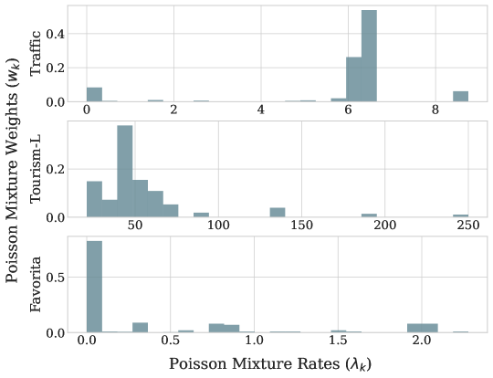
Figure 2: Poisson Mixture rates distribution for the DPMN-GroupBU model reported in Table 3. A single bottom-level series and a time step ahead in the forecast horizon is considered. The mixture distribution is capable of flexibly modeling multimodal processes, overcome Poisson regression’s limitations for aggregated data and model zero inflated processes for disaggregated data. These qualities make it exceptionally useful for hierarchical forecasting tasks.

References

- Amir & Souhaib (2016) Amir, A., & Souhaib, B. (2016). A bias and variance analysis for multistep-ahead time series forecasting. IEEE transactions on neural networks and learning systems, 27, 2162–2388. URL: https://pubmed.ncbi.nlm.nih.gov/25807572/.
- Athanasopoulos et al. (2017) Athanasopoulos, G., Hyndman, R. J., Kourentzes, N., & Petropoulos, F. (2017). Forecasting with temporal hierarchies. European Journal of Operational Research, 262, 60–74.
- Ben Taieb et al. (2017) Ben Taieb, S., Taylor, J. W., & Hyndman, R. J. (2017). Coherent probabilistic forecasts for hierarchical time series. In D. Precup, & Y. W. Teh (Eds.), Proceedings of the 34th International Conference on Machine Learning (pp. 3348–3357). PMLR volume 70 of Proceedings of Machine Learning Research. URL: http://proceedings.mlr.press/v70/taieb17a.html.
- Ben Taieb et al. (2021) Ben Taieb, S., Taylor, J. W., & Hyndman, R. J. (2021). Hierarchical probabilistic forecasting of electricity demand with smart meter data. Journal of the American Statistical Association, 116, 27–43. URL: https://doi.org/10.1080/01621459.2020.1736081. doi:10.1080/01621459.2020.1736081. arXiv:https://doi.org/10.1080/01621459.2020.1736081.
- Bergstra et al. (2011) Bergstra, J., Bardenet, R., Bengio, Y., & Kégl, B. (2011). Algorithms for hyper-parameter optimization. In J. Shawe-Taylor, R. Zemel, P. Bartlett, F. Pereira, & K. Q. Weinberger (Eds.), Advances in Neural Information Processing Systems (pp. 2546--2554). Curran Associates, Inc. volume 24. URL: https://proceedings.neurips.cc/paper/2011/file/86e8f7ab32cfd12577bc2619bc635690-Paper.pdf.
- Bishop (1994) Bishop, C. M. (1994). Mixture density networks. Technical Report Aston University Birmingham. URL: https://publications.aston.ac.uk/id/eprint/373/.
- Bolin & Wallin (2019) Bolin, D., & Wallin, J. (2019). Local scale invariance and robustness of proper scoring rules. URL: https://arxiv.org/abs/1912.05642. doi:10.48550/ARXIV.1912.05642.
- Böse et al. (2017) Böse, J.-H., Flunkert, V., Gasthaus, J., Januschowski, T., Lange, D., Salinas, D., Schelter, S., Seeger, M., & Wang, Y. (2017). Probabilistic demand forecasting at scale. Proc. VLDB Endow., 10, 1694–1705. URL: https://doi.org/10.14778/3137765.3137775. doi:10.14778/3137765.3137775.
- Cho et al. (2014) Cho, K., van Merrienboer, B., Gülçehre, Ç., Bougares, F., Schwenk, H., & Bengio, Y. (2014). Learning phrase representations using RNN encoder-decoder for statistical machine translation. Proceedings of the 2014 Conference on Empirical Methods in Natural Language Processing (EMNLP), abs/1406.1078, 1724--1734. URL: http://arxiv.org/abs/1406.1078. arXiv:1406.1078.
- Christiansen & Morris (1997) Christiansen, C. L., & Morris, C. N. (1997). Hierarchical poisson regression modeling. Journal of the American Statistical Association, 92, 618--632.
- Clevert et al. (2015) Clevert, D.-A., Unterthiner, T., & Hochreiter, S. (2015). Fast and accurate deep network learning by exponential linear units (elus). arXiv preprint arXiv:1511.07289, .
- Corporación Favorita (2018) Corporación Favorita (2018). Corporación favorita grocery sales forecasting. Kaggle Competition. URL: https://www.kaggle.com/c/favorita-grocery-sales-forecasting/.
- Diggle & Brix (2001) Diggle, P., & Brix, A. (2001). Spatio-temporal prediction for log-gaussian cox processes. Journal of the Royal Statistical Society: Series B (Statistical Methodology, 63, 823--841. doi:10.1111/1467-9868.00315.
- Diggle (2013) Diggle, P. J. (2013). Statistical Analysis of Spatial and Spatio-Temporal Point Patterns. (Third edition ed.). Routledge.
- Dua & Graff (2017) Dua, D., & Graff, C. (2017). UCI machine learning repository. URL: http://archive.ics.uci.edu/ml.
- Eisenach et al. (2021) Eisenach, C., Patel, Y., & Madeka, D. (2021). MQTransformer: Multi-Horizon Forecasts with Context Dependent and Feedback-Aware Attention. In M. F. Balcan, & M. Meila (Eds.), Submitted to Proceedings of the 38th International Conference on Machine Learning. PMLR. Working Paper version available at arXiv:2009.14799.
- Fliedner (1999) Fliedner, G. (1999). An investigation of aggregate variable time series forecast strategies with specific subaggregate time series statistical correlation. Computers and Operations Research, 26, 1133–1149. URL: https://doi.org/10.1016/S0305-0548(99)00017-9. doi:10.1016/S0305-0548(99)00017-9.
- Fotios Petropoulos et. al. (2021) Fotios Petropoulos et. al. (2021). Forecasting: theory and practice. arXiv:2012.03854.
- Gneiting & Ranjan (2011) Gneiting, T., & Ranjan, R. (2011). Comparing density forecasts using threshold-and quantile-weighted scoring rules. Journal of Business & Economic Statistics, 29, 411--422.
- Gross & Sohl (1990) Gross, C. W., & Sohl, J. E. (1990). Disaggregation methods to expedite product line forecasting. Journal of Forecasting, 9, 233--254. URL: https://onlinelibrary.wiley.com/doi/abs/10.1002/for.3980090304. doi:10.1002/for.3980090304.
- Han et al. (2021) Han, X., Dasgupta, S., & Ghosh, J. (2021). Simultaneously reconciled quantile forecasting of hierarchically related time series. In A. Banerjee, & K. Fukumizu (Eds.), Proceedings of The 24th International Conference on Artificial Intelligence and Statistics (pp. 190--198). PMLR volume 130 of Proceedings of Machine Learning Research. URL: http://proceedings.mlr.press/v130/han21a.html.
- Hollyman et al. (2021) Hollyman, R., Petropoulos, F., & Tipping, M. E. (2021). Understanding forecast reconciliation. European Journal of Operational Research, 294, 149--160. URL: https://www.sciencedirect.com/science/article/pii/S0377221721000199. doi:https://doi.org/10.1016/j.ejor.2021.01.017.
- Hong et al. (2014) Hong, T., Pinson, P., & Fan, S. (2014). Global energy forecasting competition 2012.
- Hyndman et al. (2011) Hyndman, R. J., Ahmed, R. A., Athanasopoulos, G., & Shang, H. L. (2011). Optimal combination forecasts for hierarchical time series. Computational Statistics & Data Analysis, 55, 2579 -- 2589. URL: http://www.sciencedirect.com/science/article/pii/S0167947311000971. doi:https://doi.org/10.1016/j.csda.2011.03.006.
- Hyndman & Athanasopoulos (2018) Hyndman, R. J., & Athanasopoulos, G. (2018). Forecasting: Principles and Practice. Melbourne, Australia: OTexts. Available at https://otexts.com/fpp2/.
- Hyndman & Khandakar (2008) Hyndman, R. J., & Khandakar, Y. (2008). Automatic time series forecasting: The forecast package for r. Journal of Statistical Software, Articles, 27, 1--22. URL: https://www.jstatsoft.org/v027/i03. doi:10.18637/jss.v027.i03.
- Hyndman & Koehler (2006) Hyndman, R. J., & Koehler, A. B. (2006). Another look at measures of forecast accuracy. International Journal of Forecasting, 22, 679 -- 688. URL: http://www.sciencedirect.com/science/article/pii/S0169207006000239. doi:https://doi.org/10.1016/j.ijforecast.2006.03.001.
- Hyndman et al. (2014) Hyndman, R. J., Lee, A., & Wang, E. (2014). Fast computation of reconciled forecasts for hierarchical and grouped time series. Monash Econometrics and Business Statistics Working Papers 17/14 Monash University, Department of Econometrics and Business Statistics. URL: https://ideas.repec.org/p/msh/ebswps/2014-17.html.
- Jeon et al. (2019) Jeon, J., Panagiotelis, A., & Petropoulos, F. (2019). Probabilistic forecast reconciliation with applications to wind power and electric load. European Journal of Operational Research, 279, 364--379. URL: https://www.sciencedirect.com/science/article/pii/S0377221719304242. doi:https://doi.org/10.1016/j.ejor.2019.05.020.
- Kamarthi et al. (2022) Kamarthi, H., Kong, L., Rodriguez, A., Zhang, C., & Prakash, B. (2022). PROFHIT: Probabilistic robust forecasting for hierarchical time-series. Computing Research Repository, . URL: https://arxiv.org/abs/2206.07940.
- Kingma & Ba (2014) Kingma, D. P., & Ba, J. (2014). ADAM: A method for stochastic optimization. URL: http://arxiv.org/abs/1412.6980 cite arxiv:1412.6980Comment: Published as a conference paper at the 3rd International Conference for Learning Representations (ICLR), San Diego, 2015.
- Lindsay (1988) Lindsay, B. G. (1988). Composite likelihood methods. Contemporary Mathematics, 80, 221--239.
- Madeka et al. (2018) Madeka, D., Swiniarski, L., Foster, D., Razoumov, L., Torkkola, K., & Wen, R. (2018). Sample path generation for probabilistic demand forecasting. In ICML workshop on Theoretical Foundations and Applications of Deep Generative Models.
- Makridakis et al. (2018a) Makridakis, S., Spiliotis, E., & Assimakopoulos, V. (2018a). The M4 competition: Results, findings, conclusion and way forward. International Journal of Forecasting, 34, 802 -- 808. URL: http://www.sciencedirect.com/science/article/pii/S0169207018300785. doi:https://doi.org/10.1016/j.ijforecast.2018.06.001.
- Makridakis et al. (2018b) Makridakis, S., Spiliotis, E., & Assimakopoulos, V. (2018b). Statistical and machine learning forecasting methods: Concerns and ways forward. PLOS ONE, 13, 1--26. URL: https://doi.org/10.1371/journal.pone.0194889. doi:10.1371/journal.pone.0194889.
- Makridakis et al. (2020) Makridakis, S., Spiliotis, E., & Assimakopoulos, V. (2020). The M5 accuracy competition: Results, findings and conclusions. International Journal of Forecasting, . URL: https://www.researchgate.net/publication/344487258_The_M5_Accuracy_competition_Results_findings_and_conclusions.
- Makridakis et al. (2022) Makridakis, S., Spiliotis, E., Assimakopoulos, V., Chen, Z., Gaba, A., Tsetlin, I., & Winkler, R. L. (2022). The m5 uncertainty competition: Results, findings and conclusions. International Journal of Forecasting, 38, 1365--1385. URL: https://www.sciencedirect.com/science/article/pii/S0169207021001722. doi:https://doi.org/10.1016/j.ijforecast.2021.10.009. Special Issue: M5 competition.
- Matheson & Winkler (1976) Matheson, J. E., & Winkler, R. L. (1976). Scoring rules for continuous probability distributions. Management Science, 22, 1087--1096. URL: http://www.jstor.org/stable/2629907.
- Nelder & Wedderburn (1972) Nelder, J. A., & Wedderburn, R. W. M. (1972). Generalized linear models. Journal of the Royal Statistical Society. Series A (General), 135, 370--384. URL: http://www.jstor.org/stable/2344614.
- Olivares et al. (2022) Olivares, K. G., Challu, C., Marcjasz, G., Weron, R., & Dubrawski, A. (2022). Neural basis expansion analysis with exogenous variables: Forecasting electricity prices with nbeatsx. International Journal of Forecasting, . URL: https://www.sciencedirect.com/science/article/pii/S0169207022000413. doi:https://doi.org/10.1016/j.ijforecast.2022.03.001.
- van den Oord et al. (2016) van den Oord, A., Dieleman, S., Zen, H., Simonyan, K., Vinyals, O., Graves, A., Kalchbrenner, N., Senior, A. W., & Kavukcuoglu, K. (2016). WaveNet: A generative model for raw audio. Computer Research Repository, abs/1609.03499. URL: http://arxiv.org/abs/1609.03499. arXiv:1609.03499.
- Orcutt et al. (1968) Orcutt, G. H., Watts, H. W., & Edwards, J. B. (1968). Data aggregation and information loss. The American Economic Review, 58, 773--787. URL: http://www.jstor.org/stable/1815532.
- Panagiotelis et al. (2020) Panagiotelis, A., Gamakumara, P., Athanasopoulos, G., & Hyndman, R. J. (2020). Probabilistic Forecast Reconciliation: Properties, Evaluation and Score Optimisation. Monash Econometrics and Business Statistics Working Papers 26/20 Monash University, Department of Econometrics and Business Statistics. URL: https://ideas.repec.org/p/msh/ebswps/2020-26.html.
- Panagiotelis et al. (2023) Panagiotelis, A., Gamakumara, P., Athanasopoulos, G., & Hyndman, R. J. (2023). Probabilistic forecast reconciliation: Properties, evaluation and score optimisation. European Journal of Operational Research, 306, 693--706. URL: https://www.sciencedirect.com/science/article/pii/S0377221722006087. doi:https://doi.org/10.1016/j.ejor.2022.07.040.
- Paria et al. (2021) Paria, B., Sen, R., Ahmed, A., & Das, A. (2021). Hierarchically Regularized Deep Forecasting. In Submitted to Proceedings of the 39th International Conference on Machine Learning. PMLR. Working Paper version available at arXiv:2106.07630.
- Park & Lord (2009) Park, B.-J., & Lord, D. (2009). Application of finite mixture models for vehicle crash data analysis. Accident Analysis & Prevention, 41, 683--691.
- Puwasala et al. (2018) Puwasala, G., Panagiotelis Anastasios, G., Athanasopoulos, & Hyndman, R. J. (2018). Probabilisitic Forecasts in Hierarchical Time Series. Department of Econometrics and Business Statistics Working Paper Series 11/18, .
- Rangapuram et al. (2018) Rangapuram, S. S., Seeger, M. W., Gasthaus, J., Stella, L., Wang, Y., & Januschowski, T. (2018). Deep state space models for time series forecasting. In S. Bengio, H. Wallach, H. Larochelle, K. Grauman, N. Cesa-Bianchi, & R. Garnett (Eds.), Advances in Neural Information Processing Systems. Curran Associates, Inc. volume 31. URL: https://proceedings.neurips.cc/paper/2018/file/5cf68969fb67aa6082363a6d4e6468e2-Paper.pdf.
- Rangapuram et al. (2021) Rangapuram, S. S., Werner, L. D., Benidis, K., Mercado, P., Gasthaus, J., & Januschowski, T. (2021). End-to-end learning of coherent probabilistic forecasts for hierarchical time series. In M. F. Balcan, & M. Meila (Eds.), Proceedings of the 38th International Conference on Machine Learning Proceedings of Machine Learning Research. PMLR.
- Ravuri et al. (2021) Ravuri, S. V., Lenc, K., Willson, M., Kangin, D., Lam, R., Mirowski, P., Fitzsimons, M., Athanassiadou, M., Kashem, S., Madge, S., Prudden, R., Mandhane, A., Clark, A., Brock, A., Simonyan, K., Hadsell, R., Robinson, N. H., Clancy, E., Arribas, A., & Mohamed, S. (2021). Skillful precipitation nowcasting using deep generative models of radar. Nature, 597, 672--691. URL: https://www.nature.com/articles/s41586-021-03854-z.pdf.
- Rosenblatt (1961) Rosenblatt, F. (1961). Principles of neurodynamics. perceptrons and the theory of brain mechanisms. Technical Report Cornell Aeronautical Lab Inc Buffalo NY.
- Semenoglou et al. (2021) Semenoglou, A.-A., Spiliotis, E., Makridakis, S., & Assimakopoulos, V. (2021). Investigating the accuracy of cross-learning time series forecasting methods. International Journal of Forecasting, 37, 1072--1084. URL: https://www.sciencedirect.com/science/article/pii/S0169207020301850. doi:https://doi.org/10.1016/j.ijforecast.2020.11.009.
- Shang & Hyndman (2017) Shang, H. L., & Hyndman, R. J. (2017). Grouped functional time series forecasting: An application to age-specific mortality rates. Journal of Computational and Graphical Statistics, 26, 330--343. URL: https://doi.org/10.1080/10618600.2016.1237877. doi:10.1080/10618600.2016.1237877. arXiv:https://doi.org/10.1080/10618600.2016.1237877.
- Souhaib & Bonsoo (2019) Souhaib, B., & Bonsoo, K. (2019). Regularized regression for hierarchical forecasting without unbiasedness conditions. In Proceedings of the 25th ACM SIGKDD International Conference on Knowledge Discovery & Data Mining KDD ’19 (p. 1337–1347). New York, NY, USA: Association for Computing Machinery. URL: https://doi.org/10.1145/3292500.3330976. doi:10.1145/3292500.3330976.
- Spiliotis et al. (2020) Spiliotis, E., Petropoulos, F., Kourentzes, N., & Assimakopoulos, V. (2020). Cross-temporal aggregation: Improving the forecast accuracy of hierarchical electricity consumption. Applied Energy, 261, 114339.
- Tianqi Chen et al. (2015) Tianqi Chen et al. (2015). Mxnet: A flexible and efficient machine learning library for heterogeneous distributed systems. Computing Research Repository, 1512.01274. URL: http://arxiv.org/abs/1512.01274.
- Tourism Australia, Canberra (2019) Tourism Australia, Canberra (2019). Detailed tourism Research Australia (2005), Travel by Australians. Accessed at https://robjhyndman.com/publications/hierarchical-tourism/.
- Van Erven & Cugliari (2015) Van Erven, T., & Cugliari, J. (2015). Game-theoretically optimal reconciliation of contemporaneous hierarchical time series forecasts. In Modeling and stochastic learning for forecasting in high dimensions (pp. 297--317). Springer.
- Varin et al. (2011) Varin, C., Reid, N., & Firth, D. (2011). An overview of composite likelihood methods. Statistica Sinica, 21, 5--42. URL: http://www.jstor.org/stable/24309261.
- Wen et al. (2017) Wen, R., Torkkola, K., Narayanaswamy, B., & Madeka, D. (2017). A Multi-horizon Quantile Recurrent Forecaster. In 31st Conference on Neural Information Processing Systems NIPS 2017, Time Series Workshop. URL: https://arxiv.org/abs/1711.11053. arXiv:1711.11053.
- Wickramasuriya (2023) Wickramasuriya, S. L. (2023). Probabilistic forecast reconciliation under the Gaussian framework. Accepted at Journal of Business and Economic Statistics, .
- Wickramasuriya et al. (2019) Wickramasuriya, S. L., Athanasopoulos, G., & Hyndman, R. J. (2019). Optimal forecast reconciliation for hierarchical and grouped time series through trace minimization. Journal of the American Statistical Association, 114, 804--819. URL: https://robjhyndman.com/publications/mint/. doi:10.1080/01621459.2018.1448825.
- Wikle et al. (1998) Wikle, C. K., Berliner, L. M., & Cressie, N. (1998). Hierarchical bayesian space-time models. Environmental and ecological statistics, 5, 117--154.
- Yao et al. (2007) Yao, Y., Rosasco, L., & Andrea, C. (2007). On early stopping in gradient descent learning. Constructive Approximation, 26(2), 289--315. URL: https://doi.org/10.1007/s00365-006-0663-2.
- Yu et al. (2018) Yu, B., Yin, H., & Zhu, Z. (2018). Spatio-temporal graph convolutional neural network: A deep learning framework for traffic forecasting. In Proceedings of the 27th International Joint Conference on Artificial Intelligence (IJCAI). URL: http://arxiv.org/abs/1709.04875.