Faster Perturbed Stochastic Gradient Methods for Finding Local Minima

Abstract

Escaping from saddle points and finding local minimum is a central problem in nonconvex optimization. Perturbed gradient methods are perhaps the simplest approach for this problem. However, to find $(\epsilon,\sqrt{\epsilon})$-approximate local minima, the existing best stochastic gradient complexity for this type of algorithms is $\widetilde{O}(\epsilon^{-3.5})$, which is not optimal. In this paper, we propose LENA (Last stEp shriNkAge), a faster perturbed stochastic gradient framework for finding local minima. We show that LENA with stochastic gradient estimators such as SARAH/SPIDER and STORM can find $(\epsilon,\epsilon_{H})$-approximate local minima within $\widetilde{O}(\epsilon^{-3}+\epsilon_{H}^{-6})$ stochastic gradient evaluations (or $\widetilde{O}(\epsilon^{-3})$ when $\epsilon_{H}=\sqrt{\epsilon}$). The core idea of our framework is a step-size shrinkage scheme to control the average movement of the iterates, which leads to faster convergence to the local minima.

1 Introduction

In this paper, we focus on the following optimization problem

$$\min_{\mathbf{x}\in\mathbb{R}^{d}}F(\mathbf{x}):=\mathbb{E}_{\bm{\xi}}[f(\mathbf{x};\bm{\xi})],$$ (1.1)

where $f(\mathbf{x};\bm{\xi}):\mathbb{R}^{d}\rightarrow\mathbb{R}$ is a stochastic function indexed by some random vector $\bm{\xi}$, and it is differentiable and possibly nonconvex. We consider the case where only the stochastic gradients $\nabla f(\mathbf{x};\bm{\xi})$ are accessible. (1.1) can unify a variety of stochastic optimization problems, such as finite-sum optimization and online optimization. Since in general, finding global minima of a nonconvex function could be an NP-hard problem (Hillar and Lim, 2013), one often seeks to finding an $(\epsilon,\epsilon_{H})$-approximate local minimum $\mathbf{x}$, i.e., $\|\nabla F(\mathbf{x})\|_{2}\leq\epsilon$ and $\lambda_{\min}\big{(}\nabla^{2}F(\mathbf{x})\big{)}\geq-\epsilon_{H}$, where $\nabla F(\mathbf{x})$ is the gradient of $F$ and $\lambda_{\min}\big{(}\nabla^{2}F(\mathbf{x})\big{)}$ is the smallest eigenvalue of the Hessian of $F$ at $\mathbf{x}$. In many machine learning applications such as matrix sensing and completion (Bhojanapalli et al., 2016; Ge et al., 2017), it suffices to find local minima due to the fact that all local minima are global minima.

For the case where $f$ is a deterministic function, it has been shown that vanilla gradient descent fails to find local minima efficiently since the iterates will get stuck at saddle points for exponential time (Du et al., 2017). To address this issue, the simplest idea is to add random noises as a perturbation to the stuck iterates. When second-order smoothness is assumed, Jin et al. (2017) showed that the simple perturbation step is enough for gradient descent to escape saddle points and find $(\epsilon,\sqrt{\epsilon})$-approximate local minima within $\widetilde{O}(1/\epsilon^{2})$ gradient evaluations, which matches the number of gradient evaluations for gradient descent to find $\epsilon$-stationary points. Faster convergence rate can be attained by applying accelerated gradient descent (Carmon et al., 2018; Jin et al., 2018) or cubic regularization with Hessian-vector product (Agarwal et al., 2017).

Such results suggest that perturbed gradient methods can find local minima efficiently, at least for deterministic optimization. When it comes to stochastic optimization, a natural question arises:

Can perturbed stochastic gradient methods find local minima efficiently?

To answer this question, we first look into existing results of perturbed stochastic gradient methods for finding local minima. Ge et al. (2015) showed that perturbed stochastic gradient descent can find $(\epsilon,\sqrt{\epsilon})$-approximate local minima within $\widetilde{O}(\text{poly}(\epsilon^{-1}))$ stochastic gradient evaluations. Daneshmand et al. (2018) showed that under a specific CNC condition, stochastic gradient descent is able to find $(\epsilon,\sqrt{\epsilon})$-approximate local minima within $\widetilde{O}(1/\epsilon^{5})$ stochastic gradient evaluations. Later on, Li (2019) showed that simple stochastic recursive gradient descent (SSRGD) can find $(\epsilon,\sqrt{\epsilon})$-approximate local minima within $\widetilde{O}(\epsilon^{-3.5})$ stochastic gradient evaluations, which is the state-of-the-arts to date. However, none of these results by perturbed stochastic gradient methods matches the optimal result $\widetilde{O}(\epsilon^{-3})$ for finding $\epsilon$-stationary points, achieved by stochastic recursive gradient algorithm (SARAH) (Nguyen et al., 2017b; Pham et al., 2020), stochastic path-integrated differential estimator (SPIDER) (Fang et al., 2018), stochastic nested variance-reduced gradient (SNVRG) (Zhou et al., 2018) and stochastic recursive momentum (STORM) (Cutkosky and Orabona, 2019) (See also Arjevani et al. (2019) for the lower bound results). Therefore, whether perturbed stochastic gradient methods can find local minima as efficiently as finding stationary points still remains unknown.

In this work, we give an affirmative answer to the above question. We propose a general framework named LENA, which works together with existing popular stochastic gradient estimators such as SARAH/SPIDER and STORM to find approximate local minima efficiently. We summarize our contributions as follows:

• We prove that LENA finds $(\epsilon,\epsilon_{H})$-approximate local minima within $\widetilde{O}(\epsilon^{-3}+\epsilon_{H}^{-6})$ stochastic gradient evaluations. Specifically, in the classic setting where $\epsilon_{H}=\sqrt{\epsilon}$, our LENA together with the SARAH/SPIDER estimator enjoys an $\widetilde{O}(\epsilon^{-3})$ stochastic gradient complexity, which outperforms previous best known complexity result $\widetilde{O}(\epsilon^{-3.5})$ achieved by Li (2019). Our result also matches the best possible complexity result $\widetilde{O}(\epsilon^{-3})$ achieved by negative curvature search based algorithms (Fang et al., 2018; Zhou et al., 2018), which suggests that simple methods such as perturbed stochastic gradient methods can find local minima as efficiently as the more complicated ones.

• In addition, we show that LENA with a recent proposed STORM estimator is also able to find $(\epsilon,\epsilon_{H})$-approximate local minima within $\widetilde{O}(\epsilon^{-3}+\epsilon_{H}^{-6})$ stochastic gradient evaluations.

• At the core of our LENA is a novel Last step shrinkage scheme to control the average movement of the iterates, which may be of independent interest to other related nonconvex optimization algorithm design.

To compare with previous methods, we summarized related results of stochastic first-order methods for finding local minima in Table 1.

Table 1: Comparison of different optimization algorithm for find approximate local minima of non convex online problems.

Algorithm	Gradient complexity	Classic Setting	Neon2
Neon2+Natasha2 (Allen-Zhu, 2018)	$\widetilde{\mathcal{O}}(\epsilon^{-3.25}+\epsilon^{-3}\epsilon_{H}^{-1}+\epsilon_{H}^{-5})$	$\widetilde{\mathcal{O}}(\epsilon^{-3.5})$	needed
Neon2+SCSG (Allen-Zhu and Li, 2018)	$\widetilde{\mathcal{O}}(\epsilon^{-10/3}+\epsilon^{-2}\epsilon_{H}^{-3}+\epsilon_{H}^{-5})$	$\widetilde{\mathcal{O}}(\epsilon^{-3.5})$	needed
$\text{SNVRG}^{+}$+Neon2 (Zhou et al., 2018)	$\widetilde{\mathcal{O}}(\epsilon^{-3}+\epsilon^{-2}\epsilon_{H}^{-3}+\epsilon_{H}^{-5})$	$\widetilde{\mathcal{O}}(\epsilon^{-3.5})$	needed
$\text{SPIDER-SFO}^{+}$(+Neon2)(Fang et al., 2018)	$\widetilde{\mathcal{O}}(\epsilon^{-3}+\epsilon^{-2}\epsilon_{H}^{-2}+\epsilon_{H}^{-5})$	$\widetilde{\mathcal{O}}(\epsilon^{-3})$	needed
Perturbed SGD (Ge et al., 2015)	$\text{Poly}(d,\epsilon^{-1},\epsilon_{H}^{-1})$	$\widetilde{\mathcal{O}}(\text{Poly}(\epsilon^{-1}))$	No
CNC-SGD (Daneshmand et al., 2018)	$\widetilde{\mathcal{O}}(\epsilon^{-4}+\epsilon_{H}^{-10})$	$\widetilde{\mathcal{O}}(\epsilon^{-5})$	No
SSRGD (Li, 2019)	$\widetilde{\mathcal{O}}(\epsilon^{-3}+\epsilon^{-2}\epsilon_{H}^{-3}+\epsilon^{-1}\epsilon_{H}^{-4})$	$\widetilde{\mathcal{O}}(\epsilon^{-3.5})$	No
LENA (This paper)	$\widetilde{\mathcal{O}}(\epsilon^{-3}+\epsilon_{H}^{-6})$	$\widetilde{\mathcal{O}}(\epsilon^{-3})$	No

Notation We use lower case letters to denote scalars, lower and upper case bold letters to denote vectors and matrices. We use $\|\cdot\|$ to indicate Euclidean norm. We use $\mathbb{B}_{\mathbf{x}}(r)$ to denote a Euclidean ball center at $\mathbf{x}$ with radius $r$.We also use the standard $O$ and $\Omega$ notations. We use $\lambda_{\min}(\mathbf{M})$ to denote the minimum eigenvalue of matrix $\mathbf{M}$. We say $a_{n}=O(b_{n})$ if and only if $\exists C>0,N>0,\forall n>N,a_{n}\leq Cb_{n}$; $a_{n}=\Omega(b_{n})$ if and only if $\exists C>0,N>0,\forall n>N,a_{n}\geq Cb_{n}$. The notation $\widetilde{O}$ is used to hide logarithmic factors.

2 Related Work

In this section, we review some important related works.

Variance reduction methods for finding stationary points. Our algorithm takes stochastic gradient estimators as its subroutine. Specifically, Johnson and Zhang (2013); Xiao and Zhang (2014) proposed stochastic variance reduced gradient (SVRG) for convex optimization in the finite-sum setting. Reddi et al. (2016); Allen-Zhu and Hazan (2016) analyzed SVRG for nonconvex optimization. Lei et al. (2017) proposed a new variance reduction algorithm, dubbed stochastically controlled stochastic gradient (SCSG) algorithm, which finds a $\epsilon$-stationary point within $O(\epsilon^{-10/3})$ stochastic gradient evaluations. Nguyen et al. (2017a) proposed SARAH which uses a recursive gradient estimator for convex optimization, and it was extended to nonconvex optimization in (Nguyen et al., 2017b). Fang et al. (2018) proposed a SPIDER algorithm with a recursive gradient estimator and proved an $O(\epsilon^{-3})$ stochastic gradient evaluations to find a $\epsilon$-stationary point, which matches a corresponding lower bound. Concurrently, Zhou et al. (2018) proposed an SNVRG algorithm with a nested gradient estimator and proved an $\widetilde{O}(\epsilon^{-3})$ stochastic gradient evaluations to find a $\epsilon$-stationary point. Wang et al. (2019) proposed a Spiderboost algorithm with a constant step size, achieves the same $O(\epsilon^{-3})$ gradient complexity. Pham et al. (2020) extended SARAH (Nguyen et al., 2017b) to proximal optimization and proved $O(\epsilon^{-3})$ gradient complexity for finding stationary points. Recently, Cutkosky and Orabona (2019) proposed a recursive momentum-based algorithm called STORM and proved an $\widetilde{O}(\epsilon^{-3})$ gradient complexity to find $\epsilon$-stationary points. Tran-Dinh et al. (2019) proposed a SARAH-SGD algorithm which hybrids both SGD and SARAH algorithm with an $\widetilde{O}(\epsilon^{-3})$ gradient complexity when $\epsilon$ is small. Li et al. (2020) proposed a PAGE algorithm with probabilistic gradient estimator which also attains an $\widetilde{O}(\epsilon^{-3})$ gradient complexity. In our work, we employ SARAH/SPIDER and STORM as the gradient estimator in our LENA framework since they are most representative and simple to use.

Utilizing negative curvature descent to escape from saddle points. To escape saddle points, a widely used approach is to first compute the direction of the negative curvature of the saddle point and move away along that direction. In deterministic optimization, Agarwal et al. (2017) proposed a Hessian-vector product based cubic regularization method which finds $(\epsilon,\sqrt{\epsilon})$-approximate local minima within $\widetilde{O}(\epsilon^{-7/4})$ gradient and Hessian-vector product evaluations. Carmon et al. (2018) proposed an accelerated gradient method with negative curvature finding that finds $(\epsilon,\sqrt{\epsilon})$-approximate local minima with in $\widetilde{O}(\epsilon^{-7/4})$ gradient and Hessian-vector product evaluations. Both of these complexities match the complexity $\widetilde{O}(\epsilon^{-7/4})$ achieved by perturbed accelerated gradient descent, proposed by Jin et al. (2018). In stochastic optimization, to find $(\epsilon,\epsilon_{H})$-approximate local minima, Allen-Zhu (2018) proposed a Natasha algorithm using Hessian-vector product to compute the negative curvature direction with the total computation cost of $\widetilde{O}(\epsilon^{-3.25}+\epsilon^{-3}\epsilon_{H}^{-1}+\epsilon_{H}^{-5})$. Later, Xu et al. (2017) proposed a Neon method which computes the negative curvature direction with perturbed stochastic gradients, whose total computational cost is $\widetilde{O}(\epsilon^{-10/3}+\epsilon^{-2}\epsilon_{H}^{-3}+\epsilon_{H}^{-6})$. Allen-Zhu and Li (2018) proposed a Neon2 negative curvature computation subroutine with $\widetilde{O}(\epsilon^{-10/3}+\epsilon^{-2}\epsilon_{H}^{-3}+\epsilon_{H}^{-5})$ stochastic gradient evaluations. Fang et al. (2018) then showed that SPIDER equipped with Neon2 can find $(\epsilon,\epsilon_{H})$-approximate local minima within $\widetilde{\mathcal{O}}(\epsilon^{-3}+\epsilon^{-2}\epsilon_{H}^{-2}+\epsilon_{H}^{-5})$ stochastic gradient evaluations, while independently Zhou et al. (2018) proved that SNVRG equipped with Neon2 can find $(\epsilon,\epsilon_{H})$-approximate local minima within $\widetilde{\mathcal{O}}(\epsilon^{-3}+\epsilon^{-2}\epsilon_{H}^{-3}+\epsilon_{H}^{-5})$ stochastic gradient evaluations. In contrast to this line of works, our algorithm is simpler since it does not need to use the negative curvature search routine.

3 Preliminaries

In this section, we present assumptions and definitions that will be used throughout our analysis. We first introduce the standard smoothness and Hessian Lipschitz assumptions.

Assumption 3.1

For all $\bm{\xi}$, $f(\cdot;\bm{\xi})$ is $L$-smooth and its Hessian is $\rho$-Lipschitz continuous w.r.t. $\mathbf{x}$, i.e., for any $\mathbf{x}_{1},\mathbf{x}_{2}$, we have that

$$\|\nabla f(\mathbf{x}_{1};\bm{\xi})-\nabla f(\mathbf{x}_{2};\bm{\xi})\|_{2}\leq L\|\mathbf{x}_{1}-\mathbf{x}_{2}\|_{2},\ \|\nabla^{2}f(\mathbf{x}_{1};\bm{\xi})-\nabla^{2}f(\mathbf{x}_{2};\bm{\xi})\|_{2}\leq\rho\|\mathbf{x}_{1}-\mathbf{x}_{2}\|_{2}$$

This assumption directly implies that the expected objective function $F(\mathbf{x})$ is also $L$-smooth and its Hessian is $\rho$-Lipschitz continuous. This assumption is standard for finding approximate local minima in all the results presented in Table 1.

Assumption 3.2

The squared difference between the stochastic gradient and full gradient is bounded by $\sigma^{2}<\infty$, i.e., for any $\mathbf{x},\bm{\xi}\in\mathbb{R}^{d}$, $\|\nabla f(\mathbf{x};\bm{\xi})-\nabla F(\mathbf{x})\|_{2}^{2}\leq\sigma^{2}$.

Assumption 3.2 is standard in online/stochastic optimization, including for finding second-order stationary points (Fang et al., 2018; Li, 2019), and immediately implies that the variance of the stochastic gradient is bounded by $\sigma^{2}$. It can be relaxed to be $\|\nabla f(\mathbf{x};\bm{\xi})-\nabla F(\mathbf{x})\|_{2}$ has a $\sigma$-Sub-Gaussian tail.

Let $\mathbf{x}_{0}\in\mathbb{R}^{d}$ be the starting point of the algorithm. We assume the gap between the initial function value and the optimal value is bounded.

Assumption 3.3

We have $\Delta=F(\mathbf{x}_{0})-\inf_{\mathbf{x}}F(\mathbf{x})<+\infty$.

Next, we give the formal definition of approximate local minima (a.k.a., second-order stationary points).

Definition 3.4

We call $\mathbf{x}\in\mathbb{R}^{d}$ an $(\epsilon,\epsilon_{H})$-approximate local minimum, if

$$\|\nabla F(\mathbf{x})\|_{2}\leq\epsilon,\lambda_{\min}\big{(}\nabla^{2}F(\mathbf{x})\big{)}\geq-\epsilon_{H}.$$

The definition of $(\epsilon,\epsilon_{H})$-approximate local minima is a generalization of the classical $(\epsilon,\sqrt{\epsilon})$-approximate local minima studied by Nesterov and Polyak (2006); Jin et al. (2017).

4 The LENA Framework

In this section, we present our main algorithm LENA. We begin with reviewing the mechanism of perturbed gradient descent in deterministic optimization, and then we discuss the main difficulty of extending it to the stochastic optimization case. Finally, we show how we overcome such a difficulty by presenting our LENA framework.

How does perturbed gradient descent escape from saddle points? We review the perturbed gradient descent (Jin et al., 2017) (PGD for short) with its proof roadmap, which shows how PGD finds $(\epsilon,\sqrt{\epsilon})$-approximate local minima efficiently. In general, the whole process of perturbed gradient descent can be decomposed into several epochs, and each epoch consists of two non-overlapping phases: the gradient descent phase (GD phase for short) and the Escape from saddle point phase (Escape phase for short). In each epoch, PGD starts with the GD phase by default. In the GD phase, PGD performs vanilla gradient descent to update its iterate, until at some iterate $\widetilde{\mathbf{x}}$, the norm of the gradient $\|\nabla F(\widetilde{\mathbf{x}})\|_{2}$ is less than the target accuracy $\widetilde{O}(\epsilon)$. Then PGD switches to the Escape phase. In the Escape phase, PGD first adds a uniform random noise (or Gaussian noise) to the current iterate $\widetilde{\mathbf{x}}$, then it runs $\ell_{\text{thres}}=\widetilde{O}(\epsilon^{-1/2})$ steps of vanilla gradient descent. PGD then compares the function value gap between the current iterate and the beginning iterate of Escape phase $\widetilde{\mathbf{x}}$. If the gap is less than a threshold $\mathcal{F}=\widetilde{O}(\epsilon^{1.5})$, then PGD outputs $\widetilde{\mathbf{x}}$ as the targeted local minimum. Otherwise, PGD starts a new epoch and performs gradient descent again.

To see why PGD can find $(\epsilon,\sqrt{\epsilon})$-approximate local minima within $\widetilde{O}(\epsilon^{-2})$ gradient evaluations, we do the following calculation. First, when PGD is in the GD phase, the function value decreases $\widetilde{O}(\epsilon^{2})$ per step (following the standard gradient descent analysis). When PGD is in the Escape phase, the function value decreases $\mathcal{F}/\ell_{\text{thres}}=\widetilde{O}(\epsilon^{2})$ per step on average. Therefore, the total number of steps will be bounded by $\widetilde{O}(\epsilon^{-2})$, which is of the same order as GD for finding $\epsilon$-stationary points.

Limitation of existing methods. However, extending the two-phase PGD algorithm from deterministic optimization to stochastic optimization with a competitive gradient complexity is very challenging. We take the SSRGD algorithm proposed by Li (2019) as an example, which uses SARAH/SPIDER (Fang et al., 2018) as its gradient estimator. Unlike deterministic optimization where we can access the exact function value $F(\mathbf{x})$ and gradient $\nabla F(\mathbf{x})$ defined in (1.1), in the stochastic optimization case we can only access the stochastic function $f(\mathbf{x};\bm{\xi})$ and the stochastic gradient $\nabla f(\mathbf{x};\bm{\xi})$. Therefore, in order to estimate the gradient norm $\|\nabla F(\mathbf{x})\|_{2}$ (which is required at the beginning of Escape phase), a naive approach (adapted by Li (2019)) is to sample a big batch of stochastic gradients $\nabla f(\mathbf{x};\bm{\xi}_{1}),\dots,\nabla f(\mathbf{x};\bm{\xi}_{B})$ and uses their mean to approximate $\nabla F(\mathbf{x})$. Standard concentration analysis suggests that in order to achieve an $\epsilon$-accuracy, the batch size $B$ should be in the order $\widetilde{O}(\epsilon^{-2})$. Thus, each Escape phase leads to a $\mathcal{F}=\widetilde{O}(\epsilon^{1.5})$ function value decrease with at least $\widetilde{O}(\epsilon^{-2})$ number of stochastic gradient evaluations, which contributes $\widetilde{O}(1/\epsilon^{1.5}\cdot\epsilon^{-2})=\widetilde{O}(\epsilon^{-3.5})$ gradient complexity in the end. This is already worse than the $O(\epsilon^{-3})$ gradient complexity of SPIDER for finding $\epsilon$-stationary points.

Our approach. Here we propose our LENA framework in Algorithm 1, which overcomes the aforementioned limitation. In detail, LENA inherits the two-phase structure of PGD and SSRGD, and it takes either SARAH/SPIDER or STORM (Cutkosky and Orabona, 2019) as its gradient estimator. The two gradient estimators are summarized as subroutines GradEst-SPIDER and GradEst-STORM in Algorithms 2 and 3 respectively, and we use $\mathbf{d}_{t}$ to denote their estimated gradient at iterate $\mathbf{x}_{t}$. The key improvement of LENA is that it directly takes the output of the gradient estimator GradEst to estimate the true gradient $\nabla F(\mathbf{x})$, which avoids sampling a big batch of stochastic gradients as in Li (2019) and thus saves the total gradient complexity. A similar strategy has also been adapted in Fang et al. (2018), but for the negative curvature search subroutine. However, such a strategy leads to a new problem to be solved.

Since we use $\mathbf{d}_{t}$ to directly estimate $\nabla F(\mathbf{x}_{t})$, in order to make such an estimation valid, we need to guarantee that the error between $\mathbf{d}_{t}$ and $\nabla F(\mathbf{x}_{t})$ is small enough, e.g., up to $O(\epsilon)$ accuracy. Notice that the recursive structure of SARAH/SPIDER and STORM suggests the following error bound:

$$\forall t,\ \|\mathbf{d}_{t}-\nabla F(\mathbf{x}_{t})\|_{2}^{2}=\widetilde{O}\bigg{(}\sum_{i=s_{t}}^{t-1}\|\mathbf{x}_{i+1}-\mathbf{x}_{i}\|_{2}^{2}\bigg{)},$$ (4.1)

where $s_{t}$ is some reference index only related to $t$. Therefore, in order to make the error $\|\mathbf{d}_{t}-\nabla F(\mathbf{x}_{t})\|_{2}$ small, it suffices to make the movement of the iterates $\|\mathbf{x}_{i+1}-\mathbf{x}_{i}\|_{2}$ small either individually or on average. In the GD phase, when the norm of the estimated gradient $\|\mathbf{d}_{t}\|_{2}$ is large, we use normalized gradient descent, which forces the movement $\|\mathbf{x}_{i+1}-\mathbf{x}_{i}\|_{2}=\eta_{t}\|\mathbf{d}_{t}\|_{2}=\eta$ to be small. Such an approach is also adapted by Fang et al. (2018) as a normalized gradient descent for finding either first-order stationary points or local minima. In the Escape phase, which starts at the $m_{s}$-th step. We achieve this goal by our proposed “last step shrinkage” scheme. In detail, we record the accumulative squared movement starting from $\mathbf{x}_{m_{s}+1}$ (after the perturbation step) as $D:=\sum_{i=m_{s}+1}^{t}\|\mathbf{x}_{i+1}-\mathbf{x}_{i}\|_{2}^{2}=\sum_{i=m_{s}+1}^{t}\eta_{i}^{2}\|\mathbf{d}_{i}\|_{2}^{2}$. When the average movement $D/(t-m_{s}+1)$ is large, we pull the last step size $\eta_{t}$ back to a smaller value, which forces the average movement $D/(t-m_{s}+1)$ to be small. Fortunately, such a simple step-size calibration scheme allows us to carefully control the error between $\mathbf{d}_{t}$ and $\nabla F(\mathbf{x}_{t})$, and to reduce the gradient complexity.

Here we would like to emphasize some features of our algorithm. First, our LENA is a generic framework that can use any stochastic gradient estimator satisfying (4.1). Second, following previous works (Johnson and Zhang, 2013; Fang et al., 2018; Cutkosky and Orabona, 2019), our LENA requires the access to a stochastic gradient oracle that simultaneously queries the stochastic gradients at two distinct points with the same randomness $\bm{\xi}$. That is stronger than the standard stochastic gradient oracle adapted by SGD and HVP-RVR (Arjevani et al., 2020), which only queries the stochastic gradient at a single point.

Algorithm 1 LENA

0:  Initial point $\mathbf{x}_{1}$, step size $\eta$ and $\eta_{H}$, perturbation radius $r$, threshold parameter $\ell_{\text{thres}}$, average movement $\mkern 1.5mu\overline{\mkern-1.5muD\mkern-1.5mu}\mkern 1.5mu$.

1:  $\mathbf{d}_{1}\leftarrow\texttt{GradEst}(0,{\bm{0}},{\bm{0}},\mathbf{x}_{1})$, $s\leftarrow 0$, $t\leftarrow 1$, find$\leftarrow$false

2:  while find = false do

3:     $s\leftarrow s+1$, $t_{s}\leftarrow t$, find$\leftarrow$true

4:     while $\|\mathbf{d}_{t}\|_{2}>\epsilon$ do

5:        $\eta_{t}\leftarrow\eta/\|\mathbf{d}_{t}\|_{2}$,

6:        $\mathbf{x}_{t+1}\leftarrow\mathbf{x}_{t}-\eta_{t}\mathbf{d}_{t}$, $\mathbf{d}_{t+1}\leftarrow\texttt{GradEst}(t,\mathbf{d}_{t},\mathbf{x}_{t},\mathbf{x}_{t+1})$, $t\leftarrow t+1$

7:     end while

8:     $m_{s}\leftarrow t$, $\bm{\xi}\sim\text{Uniform}\ B_{0}(r)$, $\mathbf{x}_{t+1}\leftarrow\mathbf{x}_{t}+\bm{\xi}$, $\mathbf{d}_{t+1}\leftarrow\texttt{GradEst}(t,\mathbf{d}_{t},\mathbf{x}_{t},\mathbf{x}_{t+1})$, $t\leftarrow t+1$

9:     for $k=0,\dots,\ell_{\text{thres}}-1$ do

10:        $\eta_{t}\leftarrow\eta_{H}$, $D\leftarrow\sum_{i=m_{s}}^{t}\eta_{i}^{2}\|\mathbf{d}_{i}\|_{2}^{2}$

11:        if $D>(t-m_{s}+1)\mkern 1.5mu\overline{\mkern-1.5muD\mkern-1.5mu}\mkern 1.5mu$ then

12:           Set $\eta_{t}$ such that $\sum_{i=m_{s}}^{t}\eta_{i}^{2}\|\mathbf{d}_{i}\|_{2}^{2}=(t-m_{s}+1)\mkern 1.5mu\overline{\mkern-1.5muD\mkern-1.5mu}\mkern 1.5mu$ {“Last Step Shrinkage”}

13:           $\mathbf{x}_{t+1}\leftarrow\mathbf{x}_{t}-\eta_{t}\mathbf{d}_{t}$, $\mathbf{d}_{t+1}\leftarrow\texttt{GradEst}(t,\mathbf{d}_{t},\mathbf{x}_{t},\mathbf{x}_{t+1})$, $t\leftarrow t+1$, find $\leftarrow$ false, break

14:        end if

15:        $\mathbf{x}_{t+1}\leftarrow\mathbf{x}_{t}-\eta_{t}\mathbf{d}_{t}$, $\mathbf{d}_{t+1}\leftarrow\texttt{GradEst}(t,\mathbf{d}_{t},\mathbf{x}_{t},\mathbf{x}_{t+1})$, $t\leftarrow t+1$

16:     end for

17:  end while

17:  $\mathbf{x}_{m_{s}}$

Algorithm 2 GradEst-SPIDER($t,\mathbf{d}_{t},\mathbf{x}_{t},\mathbf{x}_{t+1},b,q,B$)

0:  Big batch size $B$, mini-batch size $b$, loop length $q$

1:  if $t\ \text{mod}\ q=0$ then

2:     Generate $\bm{\xi}_{t+1}^{1},\dots,\bm{\xi}_{t+1}^{B}$. Set $\mathbf{d}_{t+1}\leftarrow\sum_{i=1}^{B}\nabla f(\mathbf{x}_{t+1};\bm{\xi}_{t+1}^{i})/B$

3:  else

4:     Generate $\bm{\xi}_{t+1}^{1},\dots,\bm{\xi}_{t+1}^{b}$. Set $\mathbf{d}_{t+1}\leftarrow\mathbf{d}_{t}+\sum_{i=1}^{b}\big{[}\nabla f(\mathbf{x}_{t+1};\bm{\xi}_{t+1}^{i})-\nabla f(\mathbf{x}_{t};\bm{\xi}_{t+1}^{i})\big{]}/b$

5:  end if

5:  $\mathbf{d}_{t+1}$

5 Main Results

In this section, we present the main theoretical results. We first present the convergence guarantee of LENA-SPIDER, which uses GradEst-SPIDER to estimate the gradient $\mathbf{d}_{t}$ in Algorithm 1.

Theorem 5.1

Under Assumptions 3.1, 3.2 and 3.3, we choose batch size $B=\widetilde{O}\big{(}\sigma^{2}\epsilon^{-2}+\sigma^{2}\rho^{2}\epsilon_{H}^{-4}\big{)}$, $b=q=\sqrt{B}$, set GD phase step size $\eta=\sigma/(2\sqrt{B}L)$, Escape phase step size $\eta_{H}=\widetilde{O}(L^{-1})$, perturbation radius $r\leq\min\big{\{}\sigma/(2\sqrt{B}L),\log(4/\delta)\eta_{H}\sigma^{2}/(2B\epsilon),\sqrt{2\log(4/\delta)\eta_{H}\sigma^{2}/(BL)}\big{\}}$, threshold $\ell_{\text{thres}}=\widetilde{O}(1/(\eta_{H}\epsilon_{H}))$ and $\mkern 1.5mu\overline{\mkern-1.5muD\mkern-1.5mu}\mkern 1.5mu=\sigma^{2}/(4BL^{2})$. Then with high probability, LENA-SPIDER can find $(\epsilon,\epsilon_{H})$-approximate local minima within $\widetilde{O}\big{(}\sigma L\Delta\epsilon^{-3}+\sigma\rho^{3}L\Delta\epsilon_{H}^{-6}\big{)}$ stochastic gradient evaluations.

Remark 5.2

In the classical setting $\epsilon=\sqrt{\epsilon_{H}}$, our result gives $\widetilde{O}(\epsilon^{-3})$ gradient complexity, which outperforms the best existing result $\widetilde{O}(\epsilon^{-3.5})$ for perturbed stochastic gradient methods achieved by SSRGD (Li, 2019). For sufficiently small $\epsilon$, Arjevani et al. (2020) proved the lower bound of gradient complexity $\Omega(\epsilon^{-3}+\epsilon_{H}^{-5})$ for any first-order stochastic methods to find $(\epsilon,\epsilon_{H})$-approximate local minima. Our results matches the lower bound $\widetilde{O}(\epsilon^{-3})$ when $\epsilon_{H}\geq\epsilon^{3/5}$. For the general case, there is still a gap in the dependency of $\epsilon_{H}$ between our result and the lower bound, and we leave to close it as future work.

Algorithm 3 GradEst-STORM($t,\mathbf{d}_{t},\mathbf{x}_{t},\mathbf{x}_{t+1},a,b,B$)

0:  Initial batch size $B$, mini batch size $b$ and weight parameter $a$.

1:  if $t=0$ then

2:     Generate $\bm{\xi}_{t+1}^{1},\dots,\bm{\xi}_{t+1}^{B}$. Set $\mathbf{d}_{t+1}\leftarrow\sum_{i=1}^{B}\nabla f(\mathbf{x}_{t+1};\bm{\xi}_{t+1}^{i})/B$

3:  else

4:     Generate $\bm{\xi}_{t+1}^{1},\dots,\bm{\xi}_{t+1}^{b}$

5:     Set $\mathbf{d}_{t+1}\leftarrow(1-a)\big{[}\mathbf{d}_{t}-\sum_{i=1}^{b}\nabla f(\mathbf{x}_{t};\bm{\xi}_{t+1}^{i})/b\big{]}+\sum_{i=1}^{b}\nabla f(\mathbf{x}_{t+1};\bm{\xi}_{t+1}^{i})/b$

6:  end if

6:  $\mathbf{d}_{t+1}$

Next, we present the convergence guarantee of LENA-STORM, which uses the gradient estimator GradEst-STORM to estimate the gradient $\mathbf{d}_{t}$ in Algorithm 1.

Theorem 5.3

Under Assumptions 3.1, 3.2 and 3.3, choose the mini batch size $b=\widetilde{O}\big{(}\sigma\epsilon^{-1}+\sigma\rho\epsilon_{H}^{-2}\big{)}$, and initial batch size $B=b^{2}$, set GD phase step size $\eta=\sigma/(2bL)$, Escape phase step size $\eta_{H}=\widetilde{O}(L^{-1})$, weight $a=56^{2}\log(4/\delta)/b$, threshold $\ell_{\text{thres}}=\widetilde{O}(1/(\eta_{H}\epsilon_{H}))$, perturbation radius $r\leq\min\big{\{}\sigma/(2bL),\log(4/\delta)^{2}\eta_{H}\sigma^{2}/(\epsilon b^{2}),\sqrt{2\log(4/\delta)^{2}\eta_{H}\sigma^{2}/(b^{2}L)}\big{\}}$, and $\mkern 1.5mu\overline{\mkern-1.5muD\mkern-1.5mu}\mkern 1.5mu=\sigma^{2}/(4b^{2}L^{2})$. Then with high probability, LENA-STORM can find $(\epsilon,\epsilon_{H})$-approximate local minima within $\widetilde{O}\big{(}\sigma L\Delta\epsilon^{-3}+\sigma\rho^{3}L\Delta\epsilon_{H}^{-6}\big{)}$ stochastic gradient evaluations.

Remark 5.4

Different from LENA-SPIDER, the estimation error $\|\mathbf{d}_{t}-\nabla F(\mathbf{x}_{t})\|_{2}$ of gradient estimator LENA-STORM is controlled by the weight parameter $a$. This allows us to come up with a simpler single-loop algorithm instead of a double-loop algorithm.

Experiments We conduct some experiments to validate the practical performance of LENA. Due to the space limit, the details of the experiment setup are deferred to Appendix A. Our experiment results suggest that although LENA does not enjoy a strictly better complexity result than existing algorithms such as NEON2-based algorithms (Xu et al., 2017; Allen-Zhu and Li, 2018), our LENA outperforms them empirically due to its simpler algorithm structure.

6 Proof Outline of the Main Results

We outline the proof of Theorem 5.1 and leave the proof of Theorem 5.3 to the appendix.

Let $\bm{\epsilon}_{t}$ denote the difference between true gradient $\nabla F(\mathbf{x}_{t})$ and the estimated gradient $\mathbf{d}_{t}$, which is $\bm{\epsilon}_{t}:=\mathbf{d}_{t}-\nabla F(\mathbf{x}_{t})$. The following lemma suggests that the estimation error $\|\bm{\epsilon}_{t}\|_{2}$ can be bounded.

Lemma 6.1

Under Assumptions 3.1 and 3.2, set $b=q=\sqrt{B}$, $\eta\leq\sigma/(2\sqrt{B}L)$, $r\leq\sigma/(2\sqrt{B}L)$ and $\mkern 1.5mu\overline{\mkern-1.5muD\mkern-1.5mu}\mkern 1.5mu\leq\sigma^{2}/(4BL^{2})$, then with probability at least $1-\delta$, for all $t$ we have

$$\|\bm{\epsilon}_{t}\|_{2}\leq\sqrt{8\log(4/\delta)}\sigma/\sqrt{B}.$$

Specifically, by the choice of $B$ in Theorem 5.1 we have that $\|\bm{\epsilon}_{t}\|_{2}\leq\epsilon/2$.

Proof 6.2 (Proof of Lemma 6.1).

By GradEst-SPIDER presented in Algorithm 2 we have

$$\bm{\epsilon}_{t+1}=\frac{1}{B}\sum_{i=1}^{B}\big{[}\nabla f(\mathbf{x}_{t+1};\bm{\xi}_{t+1}^{i})-\nabla F(\mathbf{x}_{t+1})\big{]}, t\ \text{mod}\ q=0,$$

$$\bm{\epsilon}_{t+1}=\bm{\epsilon}_{t}+\frac{1}{b}\sum_{i=1}^{b}\big{[}\nabla f(\mathbf{x}_{t+1};\bm{\xi}_{t+1}^{i})-\nabla f(\mathbf{x}_{t};\bm{\xi}_{t+1}^{i})-\nabla F(\mathbf{x}_{t+1})+\nabla F(\mathbf{x}_{t})\big{]}, t\ \text{mod}\ q\neq 0.$$

By the $L$-smoothness in Assumption 3.1 we have

$$\big{\|}\nabla f(\mathbf{x}_{t+1};\bm{\xi}_{t+1}^{i})-\nabla f(\mathbf{x}_{t};\bm{\xi}_{t+1}^{i})-\nabla F(\mathbf{x}_{t+1})+\nabla F(\mathbf{x}_{t})\big{\|}_{2}\leq 2L\|\mathbf{x}_{t+1}-\mathbf{x}_{t}\|_{2}.$$

Then by Assumption 3.2 and Azuma–Hoeffding inequality (See Lemma E.1 for details), with probability at least $1-\delta$, we have

$$\forall t>0,\ \|\bm{\epsilon}_{t+1}\|_{2}^{2}\leq 4\log(4/\delta)\bigg{(}\frac{\sigma^{2}}{B}+\frac{4L^{2}}{b}\sum_{i=\lfloor t/q\rfloor q}^{t}\|\mathbf{x}_{i+1}-\mathbf{x}_{i}\|_{2}^{2}\bigg{)}.$$ (6.1)

Notice that GradEst-SPIDER is parallel with LENA. Thus we need to further bound (6.1) by considering iterates in three different cases: (1) for step $i$ in the GD phase, by normalized gradient descent we have $\|\mathbf{x}_{i+1}-\mathbf{x}_{i}\|_{2}^{2}\leq\eta^{2}$; (2) for $i=m_{s}$ for some $s$ in the Escape phase, we have $\|\mathbf{x}_{i+1}-\mathbf{x}_{i}\|_{2}^{2}\leq r^{2}$; and (3) for the other steps in Escape phase, we have on average, $\|\mathbf{x}_{i+1}-\mathbf{x}_{i}\|_{2}^{2}\leq\mkern 1.5mu\overline{\mkern-1.5muD\mkern-1.5mu}\mkern 1.5mu$ due to the “Last Step Shrinkage” scheme. Therefore we have

$$\|\bm{\epsilon}_{t+1}\|_{2}^{2}\leq 4\log(4/\delta)\bigg{(}\frac{\sigma^{2}}{B}+\frac{4L^{2}}{b}\cdot q\cdot\max\{\eta^{2},r^{2},\mkern 1.5mu\overline{\mkern-1.5muD\mkern-1.5mu}\mkern 1.5mu\}\bigg{)}\leq\frac{8\log(4/\delta)\sigma^{2}}{B}.$$

Lemma 6.1 guarantees that with high probability $\|\nabla F(\mathbf{x}_{t})\|_{2}\leq\|\mathbf{d}_{t}\|_{2}+\epsilon$, which ensures $\|\nabla F(\mathbf{x}_{m_{s}})\|_{2}\leq 2\epsilon$ when the algorithm terminates. Next lemma bounds the function value decrease in the GD phase, which is also valid for LENA-STORM.

Lemma 6.3.

Suppose the event in Lemma 6.1 holds, $\eta\leq\epsilon/(2L)$, then for any $s$, we have

$$F(\mathbf{x}_{t_{s}})-F(\mathbf{x}_{m_{s}})\geq\frac{(m_{s}-t_{s})\eta\epsilon}{8}.$$

The choice of $\eta$ in Theorem 5.1 further implies that the loss decreases by at least $\sigma\epsilon/(16\sqrt{B}L)$ per step on average.

Proof 6.4 (Proof of Lemma 6.3).

For any $t_{s}\leq t<m_{s}$, we can show the following property (See Lemma E.2),

$$F(\mathbf{x}_{t+1})\leq F(\mathbf{x}_{t})-\frac{\eta_{t}}{2}\|\mathbf{d}_{t}\|_{2}^{2}+\frac{\eta_{t}}{2}\|\bm{\epsilon}_{t}\|_{2}^{2}+\frac{L}{2}\|\mathbf{x}_{t+1}-\mathbf{x}_{t}\|_{2}^{2}.$$ (6.2)

Plugging the update rule $\mathbf{x}_{t+1}=\mathbf{x}_{t}-\eta_{t}\mathbf{d}_{t}$ into (6.2) gives,

$$F(\mathbf{x}_{t+1}) =F(\mathbf{x}_{t})-\|\mathbf{x}_{t+1}-\mathbf{x}_{t}\|_{2}^{2}\bigg{(}\frac{1}{2\eta_{t}}-\frac{L}{2}\bigg{)}+\frac{\eta_{t}\|\bm{\epsilon}_{t}\|_{2}^{2}}{2}$$

$$\leq F(\mathbf{x}_{t})-\eta^{2}\bigg{(}\frac{1}{2\eta_{t}}-\frac{L}{2}\bigg{)}+\frac{\eta_{t}\epsilon^{2}}{8},$$

$$\leq F(\mathbf{x}_{t})-\frac{\eta\epsilon}{8}$$

where the first inequality holds due to the fact that $\eta_{t}=\eta/\|\mathbf{d}_{t}\|_{2}$ and $\|\bm{\epsilon}_{t}\|_{2}\leq\epsilon/2$, and the second inequality is by $\eta_{t}=\eta/\|\mathbf{d}_{t}\|_{2}\leq\eta/\epsilon\leq 1/(2L)$.

The following lemma shows that if $\mathbf{x}_{m_{s}}$ is a saddle point, then with high probability, the algorithm will break during the Escape phase and set find to be false. Thus, whenever $\mathbf{x}_{m_{s}}$ is not a local minima, the algorithm cannot terminate.

Lemma 6.5.

Under Assumptions 3.1 and 3.2, set perturbation radius $r\leq L\eta_{H}\epsilon_{H}/(C\rho)$,step size $\eta_{H}\leq\min\{1/(16L\log(\eta_{H}\epsilon_{H}\sqrt{d}LC^{-1}\rho^{-1}\delta^{-1}r^{-1})),1/(8CL\log\ell_{\text{thres}})\}=\widetilde{O}(L^{-1})$, $\ell_{\text{thres}}=2\log(\eta_{H}\epsilon_{H}\sqrt{d}LC^{-1}\rho^{-1}\delta^{-1}r^{-1})/(\eta_{H}\epsilon_{H})=\widetilde{O}(\eta_{H}^{-1}\epsilon_{H}^{-1})$, and $\mkern 1.5mu\overline{\mkern-1.5muD\mkern-1.5mu}\mkern 1.5mu<C^{2}L^{2}\eta_{H}^{2}\epsilon_{H}^{2}/(\rho^{2}\ell_{\text{thres}}^{2})$, where $C=O(\log(d\ell_{\text{thres}}/\delta)=\widetilde{O}(1)$. We also set $b=q=\sqrt{B}\geq 16\log(4/\delta)/(\eta_{H}^{2}\epsilon_{H}^{2})$. Then for any $s$, when $\lambda_{\min}(\nabla^{2}F(\mathbf{x}_{m_{s}}))\leq-\epsilon_{H}$, with probability at least $1-2\delta$ algorithm breaks in the Escape phase.

Proof 6.6 (Proof of Lemma 6.5).

Let $\{\mathbf{x}_{t}\},\{\mathbf{x}_{t}^{\prime}\}$ be two coupled sequences by running LENA-SPIDER  from $\mathbf{x}_{m_{s}+1},\mathbf{x}_{m_{s}+1}^{\prime}$ with $\mathbf{x}_{m_{s}+1}-\mathbf{x}_{m_{s}+1}^{\prime}=r_{0}\mathbf{e}_{1}$, where $\mathbf{x}_{m_{s}+1},\mathbf{x}_{m_{s}+1}^{\prime}\in\mathbb{B}_{\mathbf{x}_{m_{s}}}(r)$. Here $r_{0}=\delta r/\sqrt{d}$ and $\mathbf{e}_{1}$ denotes the smallest eigenvector direction of Hessian $\nabla^{2}F(\mathbf{x}_{m_{s}})$.

When $\lambda_{\min}(\nabla^{2}F(\mathbf{x}_{m_{s}}))\leq-\epsilon_{H}$, under the parameter choice in Lemma 6.5, we can show that at least one of two sequence will escape the saddle point (See Lemma E.4). To be specific, with probability at least $1-\delta$,

$$\max_{m_{s}<t<m_{s}+\ell_{\text{thres}}}\{\|\mathbf{x}_{t}-\mathbf{x}_{m_{s}+1}\|_{2},\|\mathbf{x}_{t}^{\prime}-\mathbf{x}_{m_{s}+1}^{\prime}\|_{2}\}\geq\frac{L\eta_{H}\epsilon_{H}}{C\rho}.$$ (6.3)

(6.3) suggests that for any two points $\mathbf{x}_{m_{s}+1},\mathbf{x}_{m_{s}+1}^{\prime}$ satisfying $\mathbf{x}_{m_{s}+1}-\mathbf{x}_{m_{s}+1}^{\prime}=r_{0}\mathbf{e}_{1}$, at least one of them will generate a sequence of iterates which finally move more than $L\eta_{H}\epsilon_{H}/(C\rho)$. Thus, let ${\mathcal{S}}\subseteq\mathbb{B}_{m_{s}}(r)$ be the set of $\mathbf{x}_{m_{s}+1}$ which will not generate a sequence of iterates moving more than $\frac{L\eta_{H}\epsilon_{H}}{C\rho}$, then in the direction $\mathbf{e}_{1}$, the ”thickness” of ${\mathcal{S}}$ is smaller than $r_{0}$. Simple integration shows that the ratio between the volume of ${\mathcal{S}}$ and $\mathbb{B}_{m_{s}}(r)$ is bounded by $\delta$. Therefore, since $\mathbf{x}_{m_{s}+1}$ is generated from $\mathbf{x}_{m_{s}}$ by adding a uniform random noise in ball $\mathbb{B}_{m_{s}}(r)$, we conclude that the probability for $\mathbf{x}_{m_{s}+1}$ locating in ${\mathcal{S}}$ is less than $\delta$. Applying union bound, we get with probability at least $1-2\delta$,

$$\exists m_{s}<t<m_{s}+\ell_{\text{thres}},\|\mathbf{x}_{t}-\mathbf{x}_{m_{s}+1}\|_{2}\geq\frac{L\eta_{H}\epsilon_{H}}{C\rho}.$$ (6.4)

Denote $\mathcal{E}$ as the event that the algorithm does not break in the Escape phase. Then under $\mathcal{E}$, for any $m_{s}<t<m_{s}+\ell_{\text{thres}}$, we have

$$\|\mathbf{x}_{t}-\mathbf{x}_{m_{s}+1}\|_{2}\leq\sum_{i=m_{s}+1}^{t-1}\|\mathbf{x}_{i+1}-\mathbf{x}_{i}\|_{2}\leq\sqrt{(t-m_{s})\sum_{i=m_{s}}^{t-1}\|\mathbf{x}_{i+1}-\mathbf{x}_{i}\|_{2}^{2}}\leq(t-m_{s})\sqrt{\mkern 1.5mu\overline{\mkern-1.5muD\mkern-1.5mu}\mkern 1.5mu},$$

where the first inequality is due to the triangle inequality and the second inequality is due to Cauchy-Schwarz inequality. Thus, by the choice of $\ell_{\text{thres}}$ and $\mkern 1.5mu\overline{\mkern-1.5muD\mkern-1.5mu}\mkern 1.5mu$, we have

$$\|\mathbf{x}_{t}-\mathbf{x}_{m_{s}+1}\|_{2}\leq(t-m_{s})\sqrt{\mkern 1.5mu\overline{\mkern-1.5muD\mkern-1.5mu}\mkern 1.5mu}\leq\ell_{\text{thres}}\sqrt{\mkern 1.5mu\overline{\mkern-1.5muD\mkern-1.5mu}\mkern 1.5mu}<C\cdot\frac{L\eta_{H}\epsilon_{H}}{\rho}.$$

Then by (6.4), we know that $\mathbb{P}(\mathcal{E})\leq 2\delta$. Therefore when $\lambda_{\min}(\nabla^{2}F(\mathbf{x}_{m_{s}}))\leq-\epsilon_{H}$, with probability at least $1-2\delta$, LENA breaks in the Escape phase.

Next lemma bounds the decreasing value of the function during the Escape phase if the algorithm breaks in the Escape phase(i.e. find is false).

Lemma 6.7 (localization).

Suppose the result of Lemma 6.1 holds, set $\eta_{H}\leq 1/\big{(}L\sqrt{128\log(4/\delta)}\big{)}$, $r\leq\min\big{\{}\log(4/\delta)\eta_{H}\sigma^{2}/(2B\epsilon),\sqrt{2\log(4/\delta)\eta_{H}\sigma^{2}/(BL)}\big{\}}$, and $\mkern 1.5mu\overline{\mkern-1.5muD\mkern-1.5mu}\mkern 1.5mu=\sigma^{2}/(4BL^{2})$. Suppose the algorithm breaks in the Escape phase starting at $\mathbf{x}_{m_{s}}$, then we have

$$F(\mathbf{x}_{m_{s}})-F(\mathbf{x}_{t_{s+1}})\geq(t_{s+1}-m_{s})\frac{\log(4/\delta)\eta_{H}\sigma^{2}}{B}.$$

Proof 6.8 (Proof of Lemma 6.7).

For any $m_{s}<i<t_{s+1}$, we can show the following property (See Lemma E.2),

$$F(\mathbf{x}_{i+1})\leq F(\mathbf{x}_{i})-\frac{\eta_{i}}{2}\|\mathbf{d}_{i}\|_{2}^{2}+\frac{\eta_{i}}{2}\|\bm{\epsilon}_{i}\|_{2}^{2}+\frac{L}{2}\|\mathbf{x}_{i+1}-\mathbf{x}_{i}\|_{2}^{2}.$$ (6.5)

Plugging the update rule $\mathbf{x}_{i+1}=\mathbf{x}_{i}-\eta_{i}\mathbf{d}_{i}$ into (6.5) gives,

$$F(\mathbf{x}_{i+1}) \leq F(\mathbf{x}_{i})+\frac{\eta_{i}}{2}\|\bm{\epsilon}_{i}\|_{2}^{2}-\bigg{(}\frac{1}{2\eta_{i}}-\frac{L}{2}\bigg{)}\|\mathbf{x}_{i+1}-\mathbf{x}_{i}\|_{2}^{2}$$

$$\leq F(\mathbf{x}_{i})+\frac{\eta_{H}}{2}\frac{8\log(4/\delta)\sigma^{2}}{B}-\frac{1}{4\eta_{H}}\|\mathbf{x}_{i+1}-\mathbf{x}_{i}\|_{2}^{2}$$ (6.6)

where the the second inequality holds due to Lemma 6.1 and $\eta_{i}\leq\eta_{H}\leq 1/(2L)$ for any $m_{s}<i<t_{s+1}$. Telescoping $\eqref{eq:local11}$ from $i=m_{s}+1$ to $t_{s+1}-1$, we have

$$F(\mathbf{x}_{t_{s+1}}) \leq F(\mathbf{x}_{m_{s}+1})+4\eta_{H}\log(4/\delta)(t_{s+1}-m_{s}-1)\frac{\sigma^{2}}{B}-\frac{1}{4\eta_{H}}\sum_{i=m_{s}+1}^{t_{s+1}-1}\|\mathbf{x}_{i+1}-\mathbf{x}_{i}\|_{2}^{2}.$$

Finally, we have

$$F(\mathbf{x}_{m_{s}+1})-F(\mathbf{x}_{t_{s+1}}) \geq\sum_{i=m_{s}+1}^{t_{s+1}-1}\frac{\|\mathbf{x}_{i+1}-\mathbf{x}_{i}\|_{2}^{2}}{4\eta_{H}}-4\log(4/\delta)(t_{s+1}-m_{s}-1)\eta_{H}\frac{\sigma^{2}}{B}$$

$$=(t_{s+1}-m_{s}-1)\bigg{(}\frac{\mkern 1.5mu\overline{\mkern-1.5muD\mkern-1.5mu}\mkern 1.5mu}{4\eta_{H}}-\frac{4\log(4/\delta)\eta_{H}\sigma^{2}}{B}\bigg{)}$$

$$=(t_{s+1}-m_{s}-1)\bigg{(}\frac{\sigma^{2}}{16\eta_{H}BL^{2}}-\frac{4\log(4/\delta)\eta_{H}\sigma^{2}}{B}\bigg{)}$$

$$\geq(t_{s+1}-m_{s}-1)\frac{4\log(4/\delta)\eta_{H}\sigma^{2}}{B},$$ (6.7)

where the last inequality is by the choice of $\eta_{H}\leq 1/\big{(}L\sqrt{128\log(4/\delta)}\big{)}$. For $i=m_{s}$, we have (See Lemma E.2)

$$F(\mathbf{x}_{m_{s}+1}) \leq F(\mathbf{x}_{m_{s}})+(\|\mathbf{d}_{m_{s}}\|_{2}+\|\bm{\epsilon}_{m_{s}}\|_{2}+Lr/2)r.$$ (6.8)

Plugging $\|\mathbf{d}_{m_{s}}\|_{2}\leq\epsilon$ and $\|\bm{\epsilon}_{m_{s}}\|_{2}\leq\epsilon/2$ into (6.8) gives,

$$F(\mathbf{x}_{m_{s}+1}) \leq F(\mathbf{x}_{m_{s}})+(4\epsilon+Lr/2)r\leq F(\mathbf{x}_{m_{s}})+\frac{2\log(4/\delta)\eta_{H}\sigma^{2}}{B},$$ (6.9)

where the last inequality is by the choice $r\leq\min\big{\{}\log(4/\delta)\eta_{H}\sigma^{2}/(2B\epsilon),\sqrt{2\log(4/\delta)\eta_{H}\sigma^{2}/(BL)}\big{\}}$. Combining (6.7) and (6.9) and applying $t_{s+1}-m_{s}\geq 2$ gives,

$$F(\mathbf{x}_{m_{s}})-F(\mathbf{x}_{t_{s+1}})\geq[4(t_{s+1}-m_{s}-1)-2]\frac{\log(4/\delta)\eta_{H}\sigma^{2}}{B}\geq(t_{s+1}-m_{s})\frac{\log(4/\delta)\eta_{H}\sigma^{2}}{B}.$$

Now, we can provide the proof of Theorem 5.1 .

Proof 6.9 (Proof of Theorem 5.1).

The analysis can be divided into two phases, i.e., GD phase and Escape phase. The function value will decrease at different rates in different phases.

GD phase: In this phase, $\|\mathbf{d}_{t}\|_{2}\geq\epsilon$ and $\|\bm{\epsilon}\|_{2}\leq\epsilon/2$ due to Lemma 6.1. Thus the gradients of the function are large $\|\nabla F(\mathbf{x})\|_{2}\geq\epsilon/2$. Lemma 6.3 further shows that the loss decreases by at least $\sigma\epsilon/(16\sqrt{B}L)$ on average.

Escape phase: In this phase, the starting point $\mathbf{x}_{m_{s}}$ satisfies $\|\nabla F(\mathbf{x}_{m_{s}})\|_{2}\leq\|\mathbf{d}_{m_{s}}\|_{2}+\|\bm{\epsilon}_{t}\|_{2}\leq 2\epsilon$. If $\mathbf{x}_{m_{s}}$ is a saddle point with $\lambda_{\min}(\nabla^{2}F(\mathbf{x}_{m_{s}}))\leq-\epsilon_{H}$, then by Lemma 6.5, with high probability LENA-SPIDER will break Escape phase, set find$\leftarrow$False and begin a new GD phase. Further by Lemma 6.7, the loss will decrease by at least $\log(4/\delta)\eta_{H}\sigma^{2}/B$ per step on average.

Sample Complexity: Note that the total amount for function value can decrease is at most $\Delta=F(\mathbf{x}_{0})-\inf_{\mathbf{x}}F(\mathbf{x})<+\infty$. So the algorithm must end and find an $(\epsilon,\epsilon_{H})$-approximate local minimum within $\widetilde{O}(\sqrt{B}L\Delta\sigma^{-1}\epsilon^{-1}+BL\Delta\sigma^{-2})$ iterations. Notice that on average we sample $\max\{b,B/q\}=\sqrt{B}$ examples per iteration, so the total sample complexity is $\widetilde{O}(BL\Delta\sigma^{-1}\epsilon^{-1}+B^{3/2}L\Delta\sigma^{-2})$. Plugging in the choice of $B=\widetilde{O}(\sigma^{2}\epsilon^{-2}+\sigma^{2}\rho^{2}\epsilon_{H}^{-4})$ in Theorem 5.1, we have the total gradient complexity

$$\widetilde{O}\bigg{(}\frac{\sigma L\Delta}{\epsilon^{3}}+\frac{\sigma\rho^{2}L\Delta}{\epsilon\epsilon_{H}^{4}}+\frac{\sigma\rho^{3}L\Delta}{\epsilon_{H}^{6}}\bigg{)}=\widetilde{O}\bigg{(}\frac{\sigma L\Delta}{\epsilon^{3}}+\frac{\sigma\rho^{3}L\Delta}{\epsilon_{H}^{6}}\bigg{)},$$

where the equation is due to the Young’s inequality.

7 Conclusions and Future Work

In this paper, we propose a perturbed stochastic gradient framework named LENA for finding local minima. LENA can find $(\epsilon,\epsilon_{H})$-approximate local minima within $\widetilde{O}(\epsilon^{-3}+\epsilon_{H}^{-6})$ stochastic gradient evaluations, which matches the best possible complexity results in the classical $\epsilon_{H}=\sqrt{\epsilon}$ setting. Our results show that simple perturbed gradient methods can be as efficient as more sophisticated algorithms for finding local minima in the classical setting. Recall that there still exists a mismatch between our upper bound $(\epsilon^{-3}+\epsilon_{H}^{-6})$ and the lower bound $(\epsilon^{-3}+\epsilon_{H}^{-5})$ in the general case of $\epsilon_{H}$, and we leave it as a future work to close this gap.

We thank the anonymous reviewers for their helpful comments. ZC, DZ and QG are partially supported by the National Science Foundation IIS-2008981, CAREER Award 1906169, and AWS Machine Learning Research Award. The views and conclusions contained in this paper are those of the authors and should not be interpreted as representing any funding agencies.

Appendix A Experiments

In this section, we conduct some experiments to validate our theory. We consider the symmetric matrix sensing problem. We need to recover a low-rank matrix $\mathbf{M}^{*}=\mathbf{U}^{*}(\mathbf{U}^{*})^{\top}$, where $\mathbf{U}^{*}\in\mathbb{R}^{d\times r}$. We have $n$ sensing matrix $\{\mathbf{A}_{i}\}_{i\in[n]}$ with observation $\bm{b}_{i}=\langle\mathbf{A}_{i},\mathbf{M}^{*}\rangle$. The optimization problem can be written as

$$\min_{\mathbf{U}\in\mathbb{R}^{d\times r}}f(\mathbf{U})=\frac{1}{2n}\sum_{i=1}^{n}(\langle\mathbf{A}_{i},\mathbf{U}\mathbf{U}^{\top}\rangle-\bm{b}_{i})^{2}.$$

For the data generation, we consider $d=50,r=3$ and $d=100,r=3$. Then we generate the unknown low-rank matrix $\mathbf{M}^{*}=\mathbf{U}^{*}(\mathbf{U}^{*})^{\top}$, where every element in $\mathbf{U}^{*}\in\mathbb{R}^{d\times r}$ is independently drawn from the Gaussian distribution $\mathcal{N}(0,1/d)$. We then generate $n=20d$ random sensing matrices $\{\mathbf{A}_{i}\}_{i\in[n]}$ following standard normal distribution, and thus $\bm{b}_{i}=\langle\mathbf{A}_{i},\mathbf{M}^{*}\rangle$. The global optimal value of the above optimization problem is $0$, because there is no noise in the model. Next we randomly initialize a vector $\widetilde{\mathbf{u}}_{0}\in\mathbb{R}^{d}$ from the Gaussian distribution. Then we set $\mathbf{u}_{0}=\alpha\widetilde{\mathbf{u}}_{0}$ where $\alpha$ is a small constant to guarantee that $\|\mathbf{u}_{0}\|_{2}<\lambda_{\max}(\mathbf{M}^{*})$ and set the initial input $\mathbf{U}_{0}=[\mathbf{u}_{0},{\bm{0}},{\bm{0}}]$. We have fixed initialization $\mathbf{U}_{0}$ for every optimization algorithm.

We choose our algorithm as LENA-SPIDER and take SGD, perturbed SGD (Ge et al., 2015), SPIDER (Fang et al., 2018), $\text{SPIDER-SFO}^{+}$(+Neon2) (Fang et al., 2018) and SSRGD (Li, 2019) as the baseline algorithms to compare. We evaluate the performance by objective function $\|\mathbf{U}\mathbf{U}^{\top}-\mathbf{M}^{*}\|_{F}^{2}/\|\mathbf{M}^{*}\|_{F}^{2}$ and then report the objective function value versus the number of stochastic gradient evaluations in Figure 1. We can see that without adding noise or using second-order information, SGD and SPIDER are not able to escape from saddle points (i.e., the objective function value of the converged point is far above zero). Our algorithm (LENA-SPIDER), SSRGD, Perturbed SGD and $\text{SPIDER-SFO}^{+}$(+Neon2) can escape from saddle points. Compared with SSRGD and perturbed SGD, our algorithm converges to the unknown matrix faster.

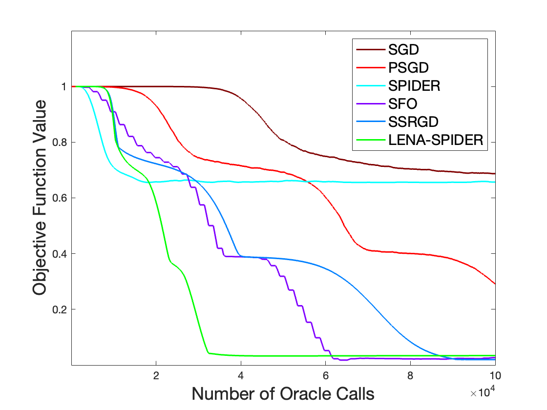
[Matrix Sensing ($d=50$)] [Matrix Sensing ($d=100$)]

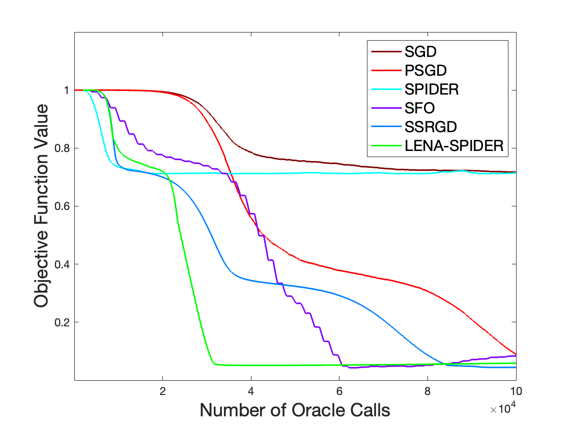
Figure 1: Convergence of different algorithms for matrix sensing: objective function value versus the number of oracle calls

Our algorithm empirically outperforms the NEON2-based algorithm $\text{SPIDER-SFO}^{+}$, which can be seen through the experiment results. The reason is that the accuracy of the negative curvature estimation is very crucial to the success of NEON2-based algorithms. However, we found that the accuracy heavily depends on the number of iterations in the NEON2 algorithm, which requires careful parameter tuning to balance the computational cost and the accuracy. In contrast, our algorithm only relies on gradient descent-type updates besides an added noise, which is easier to tune.

Appendix B Proof of Theorem 5.3

In this section we present the main proof to Theorem 5.3. We define $\bm{\epsilon}_{t}=\mathbf{d}_{t}-\nabla F(\mathbf{x}_{t})$ for simplicity.

To prove the main theorem, we need two groups of lemmas to charctrize the behavior of the Algorithm LENA-STORM.

Next lemma provides the upper bound of $\bm{\epsilon}_{t}$.

Lemma B.1.

Set $\eta\leq\sigma/(2bL)$, $r\leq\sigma/(2bL)$ and $\mkern 1.5mu\overline{\mkern-1.5muD\mkern-1.5mu}\mkern 1.5mu\leq\sigma^{2}/(4b^{2}L^{2})$, $a=56^{2}\log(4/\delta)/b$, $B=b^{2}$,$a\leq 1/4\ell_{\text{thres}}$ , with probability at least $1-2\delta$, for all $t$ we have

$$\|\bm{\epsilon}_{t}\|_{2}\leq\frac{2^{10}\log(4/\delta)\sigma}{b}.$$

Furthermore, by the choice of $b$ in Theorem 5.1 we have that $\|\bm{\epsilon}_{t}\|_{2}\leq\epsilon/2$.

Proof B.2.

See Appendix C.1.

Lemma B.3.

Suppose the event in Lemma B.1 holds and $\eta\leq\epsilon/(2L)$, then for any $s$, we have

$$F(\mathbf{x}_{t_{s}})-F(\mathbf{x}_{m_{s}})\geq\frac{(m_{s}-t_{s})\eta\epsilon}{8}.$$

Proof B.4.

The proof is the same as that of Lemma 6.3, with the fact $\|\bm{\epsilon}_{t}\|_{2}\leq\epsilon/2$ from Lemma B.1.

The choice of $\eta$ in Theorem 5.3 further implies that the loss decrease by $\sigma\epsilon/(16bL)$ on average.

Next lemma shows that if $\mathbf{x}_{m_{s}}$ is a saddle point, then with high probability, the algorithm will break during the Escape phase and set find$\leftarrow$false. Thus, whenever $\mathbf{x}_{m_{s}}$ is not a local minimum, the algorithm cannot terminate.

Lemma B.5.

Under Assumptions 3.1 and 3.2, set perturbation radius $r\leq L\eta_{H}\epsilon_{H}/\rho$, $a\leq\eta_{H}\epsilon_{H}$, $b\geq\max\{16\log(4/\delta)\eta_{H}^{-2}L^{-2}\epsilon_{H}^{-2},56^{2}\log(4/\delta)a^{-1}\}$,$\ell_{\text{thres}}=2\log(8\epsilon_{H}\sqrt{d}\rho^{-1}\delta^{-1}r^{-1})/(\eta_{H}\epsilon_{H})$, $\eta_{H}\leq\min\{1/(10L\log(8\epsilon_{H}L\rho^{-1}r_{0}^{-1})),1/(10L\log(\ell_{\text{thres}}))\}$ and $\mkern 1.5mu\overline{\mkern-1.5muD\mkern-1.5mu}\mkern 1.5mu<L^{2}\eta_{H}^{2}\epsilon_{H}^{2}/(\rho\ell_{\text{thres}}^{2})$. Then for any $s$, when $\lambda_{\min}(\nabla^{2}F(\mathbf{x}_{m_{s}}))\leq-\epsilon_{H}$, with probability at least $1-2\delta$ algorithm breaks in the Escape phase.

Proof B.6.

See Appendix C.2.

Next lemma shows that LENA-STORM decreases when it breaks.

Lemma B.7 (localization).

Suppose the event in Lemma B.1 holds, set perturbation radius $r\leq\min\big{\{}\log(4/\delta)^{2}\eta_{H}\sigma^{2}/(4b^{2}\epsilon),\sqrt{2\log(4/\delta)^{2}\eta_{H}\sigma^{2}/(b^{2}L)}\big{\}}$, $\eta_{H}\leq 1/\big{(}2^{12}L\log(4/\delta)\big{)}$, and $\mkern 1.5mu\overline{\mkern-1.5muD\mkern-1.5mu}\mkern 1.5mu=\sigma^{2}/(4b^{2}L^{2})$. Then for any $s$, when LENA-STORM breaks, then $\mathbf{x}_{m_{s}}$ satisfies

$$F(\mathbf{x}_{m_{s}})-F(\mathbf{x}_{t_{s+1}})\geq(t_{s+1}-m_{s})\frac{\log(4/\delta)^{2}\eta_{H}\sigma^{2}}{b^{2}}.$$ (B.1)

Proof B.8.

See Appendix C.3.

With all above lemmas, we prove Theorem 5.3.

Proof B.9 (Proof of Theorem 5.3).

Under the choice of parameter in Theorem 5.3, we have Lemma B.1 to B.7 hold. Now for GD phase, we know that the function value $F$ decreases by $\sigma\epsilon/(16bL)$ on average. For Escape phase, we know that the $F$ decreases by $\log(4/\delta)^{2}\eta_{H}\sigma^{2}/b^{2}$ on average. So LENA-STORM can find $(\epsilon,\epsilon_{H})$-approximate local minima within $\widetilde{O}(bL\Delta\sigma^{-1}\epsilon^{-1}+b^{2}L\Delta\sigma^{-2})$ iterations (we use the fact that $\eta_{H}=\widetilde{O}(L^{-1})$). Then the total number of stochastic gradient evaluations is bounded by $\widetilde{O}(B+b^{2}L\Delta\sigma^{-1}\epsilon^{-1}+b^{3}L\Delta\sigma^{-2})$. Plugging in the choice of $b=\widetilde{O}(\sigma\epsilon^{-1}+\sigma\rho\epsilon_{H}^{-2})$ in Theorem 5.3, we have the total sample complexity

$$\widetilde{O}\bigg{(}\frac{\sigma L\Delta}{\epsilon^{3}}+\frac{\sigma\rho^{2}L\Delta}{\epsilon\epsilon_{H}^{4}}+\frac{\sigma\rho^{3}L\Delta}{\epsilon_{H}^{6}}\bigg{)}.$$

The proof finishes by using Young’s inequality.

Appendix C Proof of Lemmas in Section B

In this section we prove lemmas in Section B. Let filtration $\mathcal{F}_{t,b}$ denote the all history before sample $\bm{\xi}_{t,b}$ at time $t\in\{0,\cdots,T\}$, then it is obvious that $\mathcal{F}_{0,1}\subseteq\mathcal{F}_{0,b}\subseteq\cdots\subseteq\mathcal{F}_{1,1}\subseteq\cdots\subseteq\mathcal{F}_{T,1}\subseteq\cdots\subseteq\mathcal{F}_{T,b}$.

We also need the following fact:

Proposition C.1.

For any $t$, we have the following equation:

$$\frac{\bm{\epsilon}_{t+1}}{(1-a)^{t+1}}-\frac{\bm{\epsilon}_{t}}{(1-a)^{t}}=\frac{1}{(1-a)^{t+1}}\sum_{i\leq b}\bm{\epsilon}_{t,i},$$

where

$$\bm{\epsilon}_{t,i} =\frac{a}{b}[\nabla f(\mathbf{x}_{t+1};\bm{\xi}_{t+1}^{i})-\nabla F(\mathbf{x}_{t+1})]$$

$$\qquad+\frac{1-a}{b}\big{[}\nabla F(\mathbf{x}_{t})-\nabla f(\mathbf{x}_{t};\bm{\xi}_{t+1}^{i})-\nabla F(\mathbf{x}_{t+1})+\nabla f(\mathbf{x}_{t+1};\bm{\xi}_{t+1}^{i})].$$

Proof C.2.

Following the update rule in LENA-STORM, we could have the update rule of $\bm{\epsilon}$ described as

$$\bm{\epsilon}_{t+1} =\frac{1-a}{b}\sum_{i\leq b}\big{[}\mathbf{d}_{t}-\nabla f(\mathbf{x}_{t};\bm{\xi}_{t+1}^{i})\big{]}+\frac{1}{b}\sum_{i\leq b}\big{[}\nabla f(\mathbf{x}_{t+1};\bm{\xi}_{t+1}^{i})-\nabla F(\mathbf{x}_{t+1})\big{]}$$

$$=\frac{a}{b}\sum_{i\leq b}[\nabla f(\mathbf{x}_{t+1};\bm{\xi}_{t+1}^{i})-\nabla F(\mathbf{x}_{t+1})]+(1-a)(\mathbf{d}_{t}-\nabla F(\mathbf{x}_{t}))$$

$$\quad+\frac{1-a}{b}\sum_{i\leq b}\big{[}\nabla F(\mathbf{x}_{t})-\nabla f(\mathbf{x}_{t};\bm{\xi}_{t+1}^{i})-\nabla F(\mathbf{x}_{t+1})+\nabla f(\mathbf{x}_{t+1};\bm{\xi}_{t+1}^{i})\big{]}$$

$$=\frac{a}{b}\sum_{i\leq b}[\nabla f(\mathbf{x}_{t+1};\bm{\xi}_{t+1}^{i})-\nabla F(\mathbf{x}_{t+1})]+(1-a)\bm{\epsilon}_{t}$$

$$\quad+\frac{1-a}{b}\sum_{i\leq b}\big{[}\nabla F(\mathbf{x}_{t})-\nabla f(\mathbf{x}_{t};\bm{\xi}_{t+1}^{i})-\nabla F(\mathbf{x}_{t+1})+\nabla f(\mathbf{x}_{t+1};\bm{\xi}_{t+1}^{i})\big{]},$$

where the last equation is by definition $\bm{\epsilon}_{t}:=\mathbf{d}_{t}-\nabla F(\mathbf{x}_{t})$. Thus we have

$$\frac{\bm{\epsilon}_{t+1}}{(1-a)^{t+1}}-\frac{\bm{\epsilon}_{t}}{(1-a)^{t}}$$

$$=\frac{1}{(1-a)^{t+1}}\Big{(}\frac{a}{b}\sum_{i\leq b}[\nabla f(\mathbf{x}_{t+1};\bm{\xi}_{t+1}^{i})-\nabla F(\mathbf{x}_{t+1})]$$

$$\quad+\frac{1-a}{b}\sum_{i\leq b}\big{[}\nabla F(\mathbf{x}_{t})-\nabla f(\mathbf{x}_{t};\bm{\xi}_{t+1}^{i})-\nabla F(\mathbf{x}_{t+1})+\nabla f(\mathbf{x}_{t+1};\bm{\xi}_{t+1}^{i})\big{]}\Big{)},$$

$$=\frac{1}{(1-a)^{t+1}}\sum_{i\leq b}\bm{\epsilon}_{t,i}.$$

C.1 Proof of Lemma B.1

Proposition C.3.

For two positive sequences $\{a_{i}\}_{i=1}^{n}$ and $\{b_{i}\}_{i=1}^{n}$. Suppose $C=\max_{i,j\in[n]}\{|a_{i}/a_{j}|\}$, $\bar{b}=\sum_{i=1}^{n}b_{i}/n$. Then we have,

$$\sum_{i=1}^{n}a_{i}b_{i}\leq\max_{i}a_{i}\cdot n\cdot\bar{b}\leq C\sum_{i=1}^{n}a_{i}\bar{b}.$$

Proof C.4 (Proof of Lemma B.1).

By Proposition C.1 we have

$$\frac{\bm{\epsilon}_{t+1}}{(1-a)^{t+1}}-\frac{\bm{\epsilon}_{t}}{(1-a)^{t}}=\frac{1}{(1-a)^{t+1}}\sum_{i\leq b}\bm{\epsilon}_{t,i}.$$

It is easy to verify that $\{\bm{\epsilon}_{t,i}\}$ forms a martingale difference sequence and

$$\|\bm{\epsilon}_{t,i}\|_{2}^{2} \leq 2\bigg{\|}\frac{a}{b}[\nabla f(\mathbf{x}_{t+1};\bm{\xi}_{t+1}^{i})-\nabla F(\mathbf{x}_{t+1})]\bigg{\|}_{2}^{2}$$

$$\quad+2\bigg{\|}\frac{1-a}{b}\big{[}\nabla F(\mathbf{x}_{t})-\nabla f(\mathbf{x}_{t};\bm{\xi}_{t+1}^{i})-\nabla F(\mathbf{x}_{t+1})+\nabla f(\mathbf{x}_{t+1};\bm{\xi}_{t+1}^{i})\big{]}\bigg{\|}_{2}^{2}$$

$$\leq\frac{2a^{2}\sigma^{2}+8(1-a)^{2}L^{2}\|\mathbf{x}_{t+1}-\mathbf{x}_{i}\|_{2}^{2}}{b^{2}},$$

where the first inequality holds due to triangle inequality, the second inequality holds due to Assumptions 3.1 and 3.2. Therefore, by Azuma-Hoeffding inequality (See Lemma E.1 for detail), with probability at least $1-\delta$, we have that for any $t>0$,

$$\bigg{\|}\frac{\bm{\epsilon}_{t}}{(1-a)^{t}}-\frac{\bm{\epsilon}_{0}}{(1-a)^{0}}\bigg{\|}_{2}^{2} \leq 4\log(4/\delta)\sum_{i=0}^{t-1}b\cdot\frac{2a^{2}\sigma^{2}+8(1-a)^{2}L^{2}\|\mathbf{x}_{i+1}-\mathbf{x}_{i}\|_{2}^{2}}{(1-a)^{2i+2}b^{2}}$$

$$=8\log(4/\delta)\sum_{i=0}^{t-1}\frac{a^{2}\sigma^{2}+4(1-a)^{2}L^{2}\|\mathbf{x}_{i+1}-\mathbf{x}_{i}\|_{2}^{2}}{(1-a)^{2i+2}b}.$$

Therefore, we have

$$\|\bm{\epsilon}_{t}\|_{2}^{2} \leq 2(1-a)^{2t}\bigg{\|}\frac{\bm{\epsilon}_{t}}{(1-a)^{t}}-\bm{\epsilon}_{0}\bigg{\|}_{2}^{2}+2(1-a)^{2t}\|\bm{\epsilon}_{0}\|_{2}^{2}$$

$$\leq\log(4/\delta)\bigg{[}\frac{64L^{2}}{b}\sum_{i=0}^{t-1}(1-a)^{2t-2i}\|\mathbf{x}_{i+1}-\mathbf{x}_{i}\|^{2}_{2}+\frac{16a\sigma^{2}}{b}\bigg{]}+2(1-a)^{2t}\|\bm{\epsilon}_{0}\|_{2}^{2}.$$ (C.1)

By Azuma-Hoeffding Inequality, we have with probability $1-\delta$,

$$\|\bm{\epsilon}_{0}\|_{2}^{2}=\bigg{\|}\frac{1}{B}\sum_{1\leq i\leq B}\Big{[}\nabla f(\mathbf{x}_{0};\bm{\xi}_{0}^{i})-\nabla F(\mathbf{x}_{0})\Big{]}\bigg{\|}_{2}^{2}\leq\frac{4\log(4/\delta)\sigma^{2}}{B}.$$

Therefore, with probability $1-2\delta$, we have

$$\|\bm{\epsilon}_{t}\|_{2}^{2} \leq\log(4/\delta)\bigg{[}\frac{64L^{2}}{b}\sum_{i=0}^{t-1}(1-a)^{2t-2i-2}\|\mathbf{x}_{i+1}-\mathbf{x}_{i}\|^{2}_{2}+\frac{16a\sigma^{2}}{b}+\frac{32(1-a)^{2t}\sigma^{2}}{B}\bigg{]}$$

$$=\frac{64L^{2}\log(4/\delta)}{b}\underbrace{\sum_{i=0}^{t-1}(1-a)^{2t-2i-2}\|\mathbf{x}_{i+1}-\mathbf{x}_{i}\|^{2}_{2}}_{I}+\frac{16a\sigma^{2}\log(4/\delta)}{b}$$ (C.2)

$$\qquad+\frac{32(1-a)^{2t}\log(4/\delta)\sigma^{2}}{B}.$$ (C.3)

We now bound $I$. Denote $S_{1}=\{i\in[t-1]|\exists j,t_{j}\leq i<m_{j}\}$, $S_{2}=\{i\in[t-1]|\exists j,i=m_{j}\}$, $S_{3}=\{i\in[t-1]|\exists j,m_{j}<i<t_{j+1}\}$, We can divide $I$ into three part,

$$I =\underbrace{\sum_{i\in S_{1}}(1-a)^{2t-2i-2}\|\mathbf{x}_{i+1}-\mathbf{x}_{i}\|^{2}_{2}}_{I_{1}}+\underbrace{\sum_{i\in S_{2}}(1-a)^{2t-2i-2}\|\mathbf{x}_{i+1}-\mathbf{x}_{i}\|^{2}_{2}}_{I_{2}}$$

$$\qquad+\underbrace{\sum_{i\in S_{3}}^{t-1}(1-a)^{2t-2i-2}\|\mathbf{x}_{i+1}-\mathbf{x}_{i}\|^{2}_{2}}_{I_{3}}.$$ (C.4)

Because $\|\mathbf{x}_{i+1}-\mathbf{x}_{i}\|_{2}=\eta_{t}\|\mathbf{d}_{i}\|_{2}=\eta$, we can bound $I_{1}$ as follows,

$$I_{1}=\eta^{2}\sum_{i\in S_{1}}(1-a)^{2t-2i-2}\leq\eta^{2}\sum_{i=0}^{\infty}(1-a)^{i}=\frac{\eta^{2}}{a}.$$ (C.5)

Because the perturbation radius is $r$, we can bound $I_{2}$ as follows,

$$I_{2}=\sum_{i\in S_{2}}(1-a)^{2t-2i-2}\|\mathbf{x}_{i+1}-\mathbf{x}_{i}\|^{2}_{2}\leq r^{2}\sum_{i\in S_{2}}(1-a)^{2t-2i-2}\leq\frac{r^{2}}{a}.$$ (C.6)

To bound $I_{3}$, we have

$$I_{3} =\sum_{i\in S_{3}}^{t-1}(1-a)^{2t-2i-2}\|\mathbf{x}_{i+1}-\mathbf{x}_{i}\|^{2}_{2}$$

$$=\sum_{s=1}^{S}\sum_{i=m_{s}+1}^{\min\{t-1,t_{s+1}-1\}}(1-a)^{2t-2i-2}\|\mathbf{x}_{i+1}-\mathbf{x}_{i}\|^{2}_{2}$$

$$\leq\sum_{s=1}^{S}(1-a)^{-2\ell_{\text{thres}}}\sum_{i=m_{s}+1}^{\min\{t-1,t_{s+1}-1\}}(1-a)^{2t-2i-2}\mkern 1.5mu\overline{\mkern-1.5muD\mkern-1.5mu}\mkern 1.5mu$$

$$=(1-a)^{-2\ell_{\text{thres}}}\sum_{i\in S_{3}}^{t-1}(1-a)^{2t-2i-2}\mkern 1.5mu\overline{\mkern-1.5muD\mkern-1.5mu}\mkern 1.5mu$$

$$\leq\frac{\mkern 1.5mu\overline{\mkern-1.5muD\mkern-1.5mu}\mkern 1.5mu(1-a)^{-2\ell_{\text{thres}}}}{a},$$ (C.7)

where $S$ satisfies $m_{S}<t-1<t_{S+1}$. The first inequality holds due to Proposition C.3 with the fact that the average of $\|\mathbf{x}_{i+1}-\mathbf{x}_{i}\|^{2}_{2}$ is bounded by $\bar{D}$, according to the LENA scheme, and $t_{s+1}-m_{s}<\ell_{\text{thres}}$, the last one holds trivially. Substituting (C.5), (C.6), (C.7) into (C.4), we have

$$I\leq\frac{\eta^{2}+r^{2}+(1-a)^{2\ell_{\text{thres}}}\mkern 1.5mu\overline{\mkern-1.5muD\mkern-1.5mu}\mkern 1.5mu}{a}.$$

Therefore (C.3) can further bounded by

$$\|\bm{\epsilon}_{t}\|_{2}^{2} \leq\frac{64L^{2}\log(4/\delta)}{b}\frac{\eta^{2}+r^{2}+(1-a)^{2\ell_{\text{thres}}}\mkern 1.5mu\overline{\mkern-1.5muD\mkern-1.5mu}\mkern 1.5mu}{a}+\frac{16a\sigma^{2}\log(4/\delta)}{b}+\frac{32(1-a)^{2t}\log(4/\delta)\sigma^{2}}{B}.$$ (C.8)

By the selection of $\eta\leq\sigma/(2bL)$, $r\leq\sigma/(2bL)$ and $\mkern 1.5mu\overline{\mkern-1.5muD\mkern-1.5mu}\mkern 1.5mu\leq\sigma^{2}/(4b^{2}L^{2})$, $a=56^{2}\log(4/\delta)/b$, $B=b^{2}$,$a\leq 1/4\ell_{\text{thres}}$, it’s easy to verify that

$$\frac{64L^{2}\log(4/\delta)}{b}\frac{\eta^{2}+r^{2}+2\mkern 1.5mu\overline{\mkern-1.5muD\mkern-1.5mu}\mkern 1.5mu}{a}\leq\frac{\sigma^{2}}{b^{2}}$$ (C.9)

$$(1-a)^{2\ell_{\text{thres}}}\geq 1-2a\ell_{\text{thres}}\geq\frac{1}{2}$$ (C.10)

$$\frac{16a\sigma^{2}\log(4/\delta)}{b}\leq\frac{224^{2}\sigma^{2}\log(4/\delta)^{2}}{b^{2}}$$ (C.11)

$$\frac{32\log(4/\delta)\sigma^{2}}{B}\leq\frac{32\log(4/\delta)\sigma^{2}}{b^{2}}.$$ (C.12)

Plugging (C.9) to (C.12) into (C.8) gives,

$$\|\bm{\epsilon}_{t}\|_{2}\leq\frac{2^{10}\log(4/\delta)\sigma}{b}.$$

C.2 Proof of Lemma B.5

Lemma C.5 (Small stuck region).

Suppose $-\gamma=\lambda_{\min}(\nabla^{2}F(\mathbf{x}_{m_{s}}))\leq-\epsilon_{H}$. Set threshold $\ell=2\log(8\epsilon_{H}\rho^{-1}r_{0}^{-1})/(\eta_{H}\gamma)$, $\eta_{H}\leq\min\{1/(10L\log(8\epsilon_{H}L\rho^{-1}r_{0}^{-1})),1/(10L\log(\ell))\}$, $a\leq\eta_{H}\gamma$, $r\leq L\eta_{H}\epsilon_{H}/\rho$. Let $\{\mathbf{x}_{t}\},\{\mathbf{x}_{t}^{\prime}\}$ be two coupled sequences by running LENA-STORM from $\mathbf{x}_{m_{s}+1},\mathbf{x}_{m_{s}+1}^{\prime}$ with $\mathbf{w}_{m_{s}+1}=\mathbf{x}_{m_{s}+1}-\mathbf{x}_{m_{s}+1}^{\prime}=r_{0}\mathbf{e}_{1}$, where $\mathbf{x}_{m_{s}+1},\mathbf{x}_{m_{s}+1}^{\prime}\in\mathbb{B}_{\mathbf{x}_{m_{s}}}(r)$, $r_{0}=\delta r/\sqrt{d}$ and $\mathbf{e}_{1}$ denotes the smallest eigenvector direction of Hessian $\nabla^{2}F(\mathbf{x}_{m_{s}})$. Moreover, let batch size $b\geq\max\{16\log(4/\delta)\eta_{H}^{-2}L^{-2}\gamma^{-2},56^{2}\log(4/\delta)a^{-1}\}$, then with probability $1-2\delta$ we have

$$\exists T\leq\ell,\max\{\|\mathbf{x}_{T}-\mathbf{x}_{0}\|_{2},\|\mathbf{x}_{T}^{\prime}-\mathbf{x}_{0}^{\prime}\|_{2}\}\geq\frac{\eta_{H}\epsilon_{H}L}{\rho}.$$

Proof C.6.

See Appendix D.1.

Proof C.7 (Proof of Lemma B.5).

We assume $\lambda_{\min}(\nabla^{2}F(\mathbf{x}_{m_{s}}))<-\epsilon_{H}$ and prove our statement by contradiction. Lemma C.5 shows that, in the random perturbation ball at least one of two points in the $\mathbf{e}_{1}$ direction will escape the saddle point if their distance is larger than $r_{0}=\frac{\delta r}{\sqrt{d}}$. Thus, the probability of the starting point $\mathbf{x}_{m_{s}+1}\sim\mathbb{B}_{\mathbf{x}_{m_{s}}}(r)$ located in the stuck region uniformly is less than $\delta$. Then with probability at least $1-2\delta$,

$$\exists m_{s}<t<m_{s}+\ell_{\text{thres}},\|\mathbf{x}_{t}-\mathbf{x}_{m_{s}}\|_{2}\geq\frac{L\eta_{H}\epsilon_{H}}{\rho}.$$ (C.13)

Suppose LENA-STORM does not break, then for any $m_{s}<t<m_{s}+\ell_{\text{thres}}$,

$$\|\mathbf{x}_{t}-\mathbf{x}_{m_{s}}\|_{2}\leq\sum_{i=m_{s}}^{t-1}\|\mathbf{x}_{i+1}-\mathbf{x}_{i}\|_{2}\leq\sqrt{(t-m_{s})\sum_{i=m_{s}}^{t-1}\|\mathbf{x}_{i+1}-\mathbf{x}_{i}\|_{2}^{2}}\leq(t-m_{s})\sqrt{\mkern 1.5mu\overline{\mkern-1.5muD\mkern-1.5mu}\mkern 1.5mu},$$

where the first inequality is due to the triangle inequality and the second inequality is due to Cauchy-Schwarz inequality. Thus, by the selection of $\mkern 1.5mu\overline{\mkern-1.5muD\mkern-1.5mu}\mkern 1.5mu$, we have

$$\|\mathbf{x}_{t}-\mathbf{x}_{m_{s}}\|_{2}\leq(t-m_{s})\sqrt{\mkern 1.5mu\overline{\mkern-1.5muD\mkern-1.5mu}\mkern 1.5mu}\leq\ell_{\text{thres}}\sqrt{\mkern 1.5mu\overline{\mkern-1.5muD\mkern-1.5mu}\mkern 1.5mu}<\frac{L\eta_{H}\epsilon_{H}}{\rho},$$

which contradicts (C.13). Therefore, we know that with probability at least $1-2\delta$, $\lambda_{\min}(\nabla^{2}F(\mathbf{x}_{m_{s}}))\geq-\epsilon_{H}$.

C.3 Proof of Lemma B.7

Proof C.8 (Proof of Lemma B.7).

Suppose $m_{s}<i<t_{s+1}$. Then with probability at least $1-\delta$, then by Lemma E.2 we have

$$F(\mathbf{x}_{i+1}) \leq F(\mathbf{x}_{i})+\frac{\eta_{i}}{2}\|\bm{\epsilon}_{i}\|_{2}^{2}-\bigg{(}\frac{1}{2\eta_{i}}-\frac{L}{2}\bigg{)}\|\mathbf{x}_{i+1}-\mathbf{x}_{i}\|_{2}^{2}$$

$$\leq F(\mathbf{x}_{i})+\frac{\eta_{H}}{2}\frac{2^{20}\log(4/\delta)^{2}\sigma^{2}}{b^{2}}-\frac{1}{4\eta_{H}}\|\mathbf{x}_{i+1}-\mathbf{x}_{i}\|_{2}^{2}$$ (C.14)

where the the second inequality holds due to Lemma B.1 and the fact that for any $m_{s}<i<t_{s+1}$, $\eta_{i}\leq\eta_{H}\leq 1/(2L)$. Taking summation of $\eqref{eq:local1}$ from $i=m_{s}+1$ to $t-1$, we have

$$F(\mathbf{x}_{t}) \leq F(\mathbf{x}_{m_{s}+1})+2^{19}\eta_{H}\log(4/\delta)^{2}(t-m_{s}-1)\frac{\sigma^{2}}{b^{2}}-\frac{1}{4\eta_{H}}\sum_{i=m_{s}+1}^{t-1}\|\mathbf{x}_{i+1}-\mathbf{x}_{i}\|_{2}^{2}.$$ (C.15)

Finally, we have

$$F(\mathbf{x}_{m_{s}+1})-F(\mathbf{x}_{t_{s+1}}) \geq\sum_{i=m_{s}+1}^{t_{s+1}-1}\frac{\|\mathbf{x}_{i+1}-\mathbf{x}_{i}\|_{2}^{2}}{4\eta_{H}}-2^{19}\log(4/\delta)^{2}(t-m_{s}-1)\eta_{H}\frac{\sigma^{2}}{b^{2}}$$

$$=(t_{s+1}-m_{s}-1)\bigg{(}\frac{\mkern 1.5mu\overline{\mkern-1.5muD\mkern-1.5mu}\mkern 1.5mu}{4\eta_{H}}-\frac{2^{19}\log(4/\delta)^{2}\eta_{H}\sigma^{2}}{b^{2}}\bigg{)}$$

$$=(t_{s+1}-m_{s}-1)\bigg{(}\frac{\sigma^{2}}{16\eta_{H}b^{2}L^{2}}-\frac{2^{19}\log(4/\delta)^{2}\eta_{H}\sigma^{2}}{b^{2}}\bigg{)}$$

$$\geq(t_{s+1}-m_{s}-1)\frac{4\log(4/\delta)^{2}\eta_{H}\sigma^{2}}{b^{2}},$$ (C.16)

where the last inequality is by the selection of $\eta_{H}\leq 1/\big{(}2^{12}L\log(4/\delta)\big{)}$. For $i=m_{s}$, by Lemma E.2 we have

$$F(\mathbf{x}_{m_{s}+1}) \leq F(\mathbf{x}_{t})+(2\|\mathbf{d}_{t}\|_{2}+2\|\bm{\epsilon}_{t}\|_{2}+Lr/2)r$$

$$\leq F(\mathbf{x}_{m_{s}})+(4\epsilon+Lr/2)r$$

$$\leq F(\mathbf{x}_{m_{s}})+\frac{2\log(4/\delta)^{2}\eta_{H}\sigma^{2}}{b^{2}},$$ (C.17)

where the last inequality is by $r\leq\min\big{\{}\log(4/\delta)^{2}\eta_{H}\sigma^{2}/(4b^{2}\epsilon),\sqrt{2\log(4/\delta)^{2}\eta_{H}\sigma^{2}/(b^{2}L)}\big{\}}$.

Combining (C.16) and (C.17) we have that

$$F(\mathbf{x}_{m_{s}})-F(\mathbf{x}_{t_{s+1}}) =F(\mathbf{x}_{m_{s}})-F(\mathbf{x}_{m_{s}+1})+F(\mathbf{x}_{m_{s}+1})-F(\mathbf{x}_{t_{s+1}})$$

$$\geq(t_{s+1}-m_{s}-1)\frac{4\log(4/\delta)^{2}\eta_{H}\sigma^{2}}{b^{2}}-\frac{2\log(4/\delta)^{2}\eta_{H}\sigma^{2}}{b^{2}}$$

$$\geq(t_{s+1}-m_{s})\frac{\log(4/\delta)^{2}\eta_{H}\sigma^{2}}{b^{2}},$$

where we use the fact that $t_{s+1}-m_{s}\geq 2$.

Appendix D Proof of Lemmas in Section C

D.1 Proof of Lemma C.5

Define $\mathbf{w}_{t}:=\mathbf{x}_{t}-\mathbf{x}_{t}^{\prime}$ as the distance between the two coupled sequences. By the construction, we have that $\mathbf{w}_{0}=r_{0}\mathbf{e}_{1}$, where $\mathbf{e}_{1}$ is the smallest eigenvector direction of Hessian $\mathcal{H}:=\nabla^{2}F(\mathbf{x}_{m_{s}})$.

$$\mathbf{w}_{t} =\mathbf{w}_{t-1}-\eta(\mathbf{d}_{t-1}-\mathbf{d}_{t-1}^{\prime})$$

$$=\mathbf{w}_{t-1}-\eta(\nabla F(\mathbf{x}_{t-1})-\nabla F(\mathbf{x}_{t-1}^{\prime})+\mathbf{d}_{t-1}-F(\mathbf{x}_{t-1})-\mathbf{d}_{t-1}^{\prime}+\nabla F(\mathbf{x}_{t-1}^{\prime}))$$

$$=\mathbf{w}_{t-1}-\eta\bigg{[}(\mathbf{x}_{t-1}-\mathbf{x}_{t-1}^{\prime})\int_{0}^{1}\nabla^{2}F(\mathbf{x}_{t-1}^{\prime}+\theta(\mathbf{x}_{t-1}-\mathbf{x}_{t-1}^{\prime}))d\theta$$

$$\qquad+\mathbf{d}_{t-1}-F(\mathbf{x}_{t-1})-\mathbf{d}_{t-1}^{\prime}+F(\mathbf{x}_{t-1}^{\prime})\bigg{]}$$

$$=(1-\eta\mathcal{H})\mathbf{w}_{t-1}-\eta(\Delta_{t-1}\mathbf{w}_{t-1}+\mathbf{y}_{t-1}),$$

where

$$\Delta_{t-1}:=\int_{0}^{1}\big{(}\nabla^{2}F(\mathbf{x}_{t-1}^{\prime}+\theta(\mathbf{x}_{t-1}-\mathbf{x}_{t-1}^{\prime}))-\mathcal{H}\big{)}d\theta,$$

$$\mathbf{y}_{t-1}:=\mathbf{d}_{t-1}-\nabla F(\mathbf{x}_{t-1})-\mathbf{d}_{t-1}^{\prime}+\nabla F(\mathbf{x}_{t-1}^{\prime})=\bm{\epsilon}_{t-1}-\bm{\epsilon}_{t-1}^{\prime}.$$

Recursively applying the above equation, we get

$$\mathbf{w}_{t}=(1-\eta\mathcal{H})^{t-m_{s}-1}\mathbf{w}_{m_{s}+1}-\eta\sum_{\tau=m_{s}+1}^{t-1}(1-\eta\mathcal{H})^{t-1-\tau}(\Delta_{\tau}\mathbf{w}_{\tau}+\mathbf{y}_{\tau}).$$ (D.1)

We want to show that the first term of (D.1) dominates the second term. Next Lemma is essential for the proof of Lemma C.5, which bounds the norm of $\mathbf{y}_{t}$.

Lemma D.1.

Under Assumption 3.1, we have following inequality holds,

$$\|\mathbf{y}_{t}\|_{2} \leq 2\sqrt{\log(4/\delta)}b^{-1/2}a^{-1/2}\Big{(}2L\max_{m_{s}<\tau<t}\|\mathbf{w}_{\tau+1}-\mathbf{w}_{\tau}\|_{2}$$

$$\quad+\max_{m_{s}<\tau\leq t}(2aL+4\rho D_{\tau})\cdot\max_{m_{s}<\tau\leq t}\|\mathbf{w}_{\tau}\|_{2}\Big{)}+4\sqrt{\log(4/\delta)}b^{-1/2}Lr_{0},$$ (D.2)

where $D_{\tau}=\max\{\|\mathbf{x}_{\tau}-\mathbf{x}_{m_{s}}\|_{2},\|\mathbf{x}_{\tau}^{\prime}-\mathbf{x}_{m_{s}}\|_{2}\}$.

Proof D.2 (Proof of Lemma D.1).

By Proposition C.1, we have that

$$\frac{\mathbf{y}_{t+1}}{(1-a)^{t+1}}-\frac{\mathbf{y}_{t}}{(1-a)^{t}} =\frac{\bm{\epsilon}_{t+1}}{(1-a)^{t+1}}-\frac{\bm{\epsilon}_{t}}{(1-a)^{t}}-\frac{\bm{\epsilon}_{t+1}^{\prime}}{(1-a)^{t+1}}+\frac{\bm{\epsilon}_{t}^{\prime}}{(1-a)^{t}}$$

$$=\frac{1}{(1-a)^{t+1}}\sum_{i\leq b}[\bm{\epsilon}_{t,i}-\bm{\epsilon}_{t,i}^{\prime}],$$

where $\bm{\epsilon}_{t,i}$ is the same as that in Proposition C.1:

$$\bm{\epsilon}_{t,i} =\frac{a}{b}[\nabla f(\mathbf{x}_{t+1};\bm{\xi}_{t+1}^{i})-\nabla F(\mathbf{x}_{t+1})]$$

$$\qquad+\frac{1-a}{b}\big{[}\nabla F(\mathbf{x}_{t})-\nabla f(\mathbf{x}_{t};\bm{\xi}_{t+1}^{i})-\nabla F(\mathbf{x}_{t+1})+\nabla f(\mathbf{x}_{t+1};\bm{\xi}_{t+1}^{i})]$$

$$=\frac{1}{b}[\nabla f(\mathbf{x}_{t+1};\bm{\xi}_{t+1}^{i})-\nabla F(\mathbf{x}_{t+1})]+\frac{1-a}{b}\big{[}\nabla F(\mathbf{x}_{t})-\nabla f(\mathbf{x}_{t};\bm{\xi}_{t+1}^{i})],$$ (D.3)

where we rewrite $\bm{\epsilon}_{t,i}$ as (D.3) because now we want bound the $\bm{\epsilon}_{t}-\bm{\epsilon}_{t}^{\prime}$ by the distance between two sequence. $\bm{\epsilon}_{t,i}^{\prime}$ is defined similarly as follows

$$\bm{\epsilon}_{t,i}^{\prime} =\frac{1}{b}[\nabla f(\mathbf{x}_{t+1};\bm{\xi}_{t+1}^{i})-\nabla F(\mathbf{x}_{t+1})]+\frac{1-a}{b}\big{[}\nabla F(\mathbf{x}_{t})-\nabla f(\mathbf{x}_{t};\bm{\xi}_{t+1}^{i})].$$

It is easy to verify that $\{\bm{\epsilon}_{t,i}-\bm{\epsilon}_{t,i}^{\prime}\}$ forms a martingale difference sequence. We now bound $\|\bm{\epsilon}_{t,i}-\bm{\epsilon}_{t,i^{\prime}}\|_{2}^{2}$. Denote $\mathcal{H}_{t+1,i}=\nabla^{2}f(\mathbf{x}_{m_{s}};\bm{\xi}_{t+1}^{i})$, then we introduce two terms

$$\Delta_{t+1,i}:=\int_{0}^{1}\big{(}\nabla^{2}f(\mathbf{x}_{t+1}^{\prime}+\theta(\mathbf{x}_{t+1}-\mathbf{x}_{t+1}^{\prime});\bm{\xi}_{t+1}^{i})-\mathcal{H}_{t+1,i}\big{)}d\theta$$

$$\widehat{\Delta}_{t+1,i}:=\int_{0}^{1}\big{(}\nabla^{2}f(\mathbf{x}_{t}^{\prime}+\theta(\mathbf{x}_{t}-\mathbf{x}_{t}^{\prime});\bm{\xi}_{t+1}^{i})-\mathcal{H}_{t+1,i}\big{)}d\theta,$$

By Assumption 3.1, we have $\|\Delta_{t+1,i}\|_{2}\leq\rho\max_{\theta\in[0,1]}\|\mathbf{x}_{t+1}^{\prime}+\theta(\mathbf{x}_{t+1}-\mathbf{x}_{t+1}^{\prime})-\mathbf{x}_{m_{s}+1}\|_{2}\leq\rho D_{t+1}$, similarly we have $\|\widehat{\Delta}_{t+1,i}\|_{2}\leq\rho D_{t}$ and $\Delta_{t+1}\leq\rho D_{t+1}$.

Now we bound $\bm{\epsilon}_{t,i}-\bm{\epsilon}_{t,i}^{\prime}$,

$$b(\bm{\epsilon}_{t,i}-\bm{\epsilon}_{t,i}^{\prime}) =\Big{(}[\nabla f(\mathbf{x}_{t+1};\bm{\xi}_{t+1}^{i})-\nabla F(\mathbf{x}_{t+1})]+(1-a)\big{[}\nabla F(\mathbf{x}_{t})-\nabla f(\mathbf{x}_{t};\bm{\xi}_{t+1}^{i})\big{]}\Big{)}$$

$$\quad-\Big{(}[\nabla f(\mathbf{x}_{t+1}^{\prime};\bm{\xi}_{t+1}^{i})-\nabla F(\mathbf{x}_{t+1}^{\prime})]-(1-a)\big{[}\nabla F(\mathbf{x}_{t}^{\prime})-\nabla f(\mathbf{x}_{t}^{\prime};\bm{\xi}_{t+1}^{i})\big{]}\Big{)}$$

$$=\big{(}\mathcal{H}_{t+1,i}\mathbf{w}_{t+1}+\Delta_{t+1,i}\mathbf{w}_{t+1}-\mathcal{H}\mathbf{w}_{t+1}-\Delta_{t+1}\mathbf{w}_{t+1}+(1-a)\mathcal{H}\mathbf{w}_{t}$$

$$\quad+(1-a)\Delta_{t}\mathbf{w}_{t}-(1-a)\mathcal{H}_{t+1,i}\mathbf{w}_{t}-(1-a)\widehat{\Delta}_{t+1,i}\mathbf{w}_{t}\big{)}$$

$$=\big{(}\mathcal{H}_{t+1,i}-\mathcal{H}\big{)}\big{(}\mathbf{w}_{t+1}-(1-a)\mathbf{w}_{t}\big{)}+\big{(}\Delta_{t+1,i}-\Delta_{t+1}\big{)}\mathbf{w}_{t+1}$$

$$\qquad+(1-a)\big{(}\Delta_{t}-\widehat{\Delta}_{t+1,i})\mathbf{w}_{t}.$$ (D.4)

This implies the LHS of (D.4) has the following bound.

$$\|b(\bm{\epsilon}_{t,i}-\bm{\epsilon}_{t,i}^{\prime})\|_{2} \leq 2L\|\mathbf{w}_{t+1}-(1-a)\mathbf{w}_{t}\|_{2}+2\rho D_{t+1}^{x}\|\mathbf{w}_{t+1}\|_{2}+2\rho D_{t}^{x}\|\mathbf{w}_{t}\|_{2}$$

$$\leq 2L\|\mathbf{w}_{t+1}-\mathbf{w}_{t}\|_{2}+2\rho D_{t+1}^{x}\|\mathbf{w}_{t+1}\|_{2}+(2aL+2\rho D_{t}^{x})\|\mathbf{w}_{t}\|_{2}$$

$$\leq\underbrace{2L\max_{m_{s}<\tau<t}\|\mathbf{w}_{\tau+1}-\mathbf{w}_{\tau}\|_{2}+\max_{m_{s}<\tau\leq t}(2aL+4\rho D_{\tau})\cdot\max_{m_{s}<\tau\leq t}\|\mathbf{w}_{\tau}\|_{2}}_{M}$$

where the first inequality is by the gradient Lipschitz Assumption and Hessian Lipschitz Assumption 3.1, the second inequality is by triangle inequality. Therefore we have

$$\|\bm{\epsilon}_{t,i}-\bm{\epsilon}_{t,i}^{\prime}\|_{2}^{2}\leq\frac{M^{2}}{b^{2}}$$

Furthermore, by Azuma Hoeffding inequality(See Lemma E.1 for detail), with probability at least $1-\delta$, we have that for any $t>0$,

$$\bigg{\|}\frac{\mathbf{y}_{t}}{(1-a)^{t}}-\frac{\mathbf{y}_{m_{s}+1}}{(1-a)^{m_{s}+1}}\bigg{\|}_{2}^{2} =\bigg{\|}\sum_{\tau=m_{s}+1}^{t-1}\bigg{(}\frac{\mathbf{y}_{\tau+1}}{(1-a)^{\tau+1}}-\frac{\mathbf{y}_{\tau}}{(1-a)^{\tau}}\bigg{)}\bigg{\|}_{2}^{2}$$

$$=\bigg{\|}\sum_{\tau=m_{s}+1}^{t-1}\bigg{(}\frac{1}{(1-a)^{\tau+1}}\sum_{i\leq b}[\bm{\epsilon}_{\tau,i}-\bm{\epsilon}_{\tau,i}^{\prime}]\bigg{)}\bigg{\|}_{2}^{2}$$

$$\leq 4\log(4/\delta)\bigg{(}\sum_{i=m_{s}+1}^{t-1}b\cdot\frac{M^{2}}{(1-a)^{2\tau+2}b^{2}}\bigg{)}.$$

Multiply $(1-a)^{2t}$ on both side, we get

$$\|\mathbf{y}_{t}-(1-a)^{t-m_{s}-1}\mathbf{y}_{m_{s}+1}\|_{2}^{2} \leq 4b^{-1}\log(4/\delta)\sum_{\tau=m_{s}+1}^{t-1}(1-a)^{2t-2\tau-2}M^{2}$$

$$\leq 4\log(4/\delta)b^{-1}a^{-1}M^{2},$$

where the last inequality is by $\sum_{i=0}^{t-1}(1-a)^{2t-2i-2}\leq a^{-1}$. Furthermore, by triangle inequality we have

$$\|\mathbf{y}_{t}\|_{2}\leq 2\sqrt{\log(4/\delta)}b^{-1/2}a^{-1/2}M+(1-a)^{t-m_{s}-1}\|\mathbf{y}_{m_{s}+1}\|_{2}.$$ (D.5)

Next, we have $\|\nabla f(\mathbf{x}_{m_{s}+1};\bm{\xi}_{m_{s}+1}^{i})-\nabla F(\mathbf{x}_{m_{s}+1}^{\prime})-\nabla f(\mathbf{x}_{m_{s}+1}^{\prime};\bm{\xi}_{m_{s}+1}^{i})+\nabla F(\mathbf{x}_{m_{s}+1}^{\prime})\|_{2}\leq 2Lr_{0}$ due to Assumption 3.1. Then by Azuma Inequality (See Lemma E.1), we have with probability at least $1-\delta$,

$$\|\mathbf{y}_{m_{s}+1}\|_{2}^{2} =\|\mathbf{d}_{m_{s}+1}-\nabla F(\mathbf{x}_{m_{s}+1})-\mathbf{d}_{m_{s}+1}^{\prime}+\nabla F(\mathbf{x}_{m_{s}+1}^{\prime})\|_{2}^{2}$$

$$=\bigg{\|}\frac{1}{b}\sum_{i\leq b}[\nabla f(\mathbf{x}_{m_{s}+1};\bm{\xi}_{m_{s}+1}^{i})-\nabla F(\mathbf{x}_{m_{s}+1}^{\prime})-\nabla f(\mathbf{x}_{m_{s}+1}^{\prime};\bm{\xi}_{m_{s}+1}^{i})+\nabla F(\mathbf{x}_{m_{s}+1}^{\prime})]\bigg{\|}_{2}^{2}$$

$$\leq\frac{4\log(4/\delta)4L^{2}r_{0}^{2}}{b}.$$ (D.6)

Plugging (D.6) into (D.5) gives

$$\|\mathbf{y}_{t}\|_{2} \leq 2\sqrt{\log(4/\delta)}b^{-1/2}a^{-1/2}\Big{(}2L\max_{m_{s}<\tau<t}\|\mathbf{w}_{\tau+1}-\mathbf{w}_{\tau}\|_{2}$$

$$\quad+\max_{m_{s}<\tau\leq t}(2aL+4\rho D_{\tau})\cdot\max_{m_{s}<\tau\leq t}\|\mathbf{w}_{\tau}\|_{2}\Big{)}+4\sqrt{\log(4/\delta)}b^{-1/2}Lr_{0}.$$

Now we can give a proof of Lemma C.5.

Proof D.3 (Proof of Lemma C.5).

We proof it by induction that

1. $\frac{1}{2}(1+\eta_{H}\gamma)^{t-m_{s}-1}r_{0}\leq\|\mathbf{w}_{t}\|_{2}\leq\frac{3}{2}(1+\eta_{H}\gamma)^{t-m_{s}-1}r_{0}.$

2. $\|y_{t}\|_{2}\leq 2\eta_{H}\gamma L(1+\eta_{H}\gamma)^{t-m_{s}-1}r_{0}$.

First for $t=m_{s}+1$, we have $\|\mathbf{w}_{m_{s}+1}\|_{2}=r_{0}$, $\|y_{m_{s}+1}\|_{2}\leq\sqrt{16b^{-1}\log(4/\delta)L^{2}r_{0}^{2}}\leq 2\eta_{H}\gamma Lr_{0}$(See (D.6)), where $b\geq 2\eta_{H}^{-2}\gamma^{-2}\sqrt{\log(4/\delta)}$. Assume they hold for all $m_{s}<\tau<t$, we now prove they hold for t. We bound $\mathbf{w}_{t}$ first, we only need to show that second term of (D.1) is bounded by $\frac{1}{2}(1+\eta_{H}\gamma)^{t}r_{0}$.

$$\bigg{\|}\eta_{H}\sum_{\tau=m_{s}+1}^{t-1}(1-\eta_{H}\mathcal{H})^{t-1-\tau}(\Delta_{\tau}\mathbf{w}_{\tau}+\mathbf{y}_{\tau})\bigg{\|}_{2}$$

$$\leq\eta_{H}\sum_{\tau=m_{s}+1}^{t-1}(1+\eta_{H}\gamma)^{t-1-\tau}(\|\Delta_{\tau}\|_{2}\|\mathbf{w}_{\tau}\|_{2}+\|\mathbf{y}_{\tau}\|_{2})$$

$$\leq\eta_{H}\sum_{\tau=m_{s}+1}^{t-1}(1+\eta_{H}\gamma)^{t-m_{s}-2}r_{0}(\frac{3}{2}\|\Delta_{\tau}\|_{2}+2\eta_{H}\gamma L)$$

$$\leq\eta_{H}\sum_{\tau=m_{s}+1}^{t-1}(1+\eta_{H}\gamma)^{t-m_{s}-2}r_{0}(3\eta_{H}\epsilon_{H}L+2\eta_{H}\gamma L)$$

$$=\eta_{H}\ell(1+\eta_{H}\gamma)^{t-m_{s}-2}r_{0}\cdot 5\eta_{H}\gamma L$$

$$\leq 10\log(8\epsilon_{H}\rho^{-1}r_{0}^{-1})\eta_{H}L(1+\eta_{H}\gamma)^{t-m_{s}-2}r_{0}$$

$$\leq\frac{1}{2}(1+\eta_{H}\gamma)^{t-m_{s}-1}r_{0},$$

where the first inequality is by the eigenvalue assumption over $\mathcal{H}$, the second inequality is by the Induction hypothesis, the third inequality is by $\|\Delta_{\tau}\|_{2}\leq\rho D_{\tau}=\rho\max\{\|\mathbf{x}_{\tau}-\mathbf{x}_{m_{s}}\|_{2},\|\mathbf{x}_{\tau}^{\prime}-\mathbf{x}_{m_{s}}\|_{2}\}\leq\eta_{H}\epsilon_{H}L+r\rho\leq 2\eta_{H}\epsilon_{H}L$, the fourth inequality is by the choice of $t-m_{s}-1\leq\ell\leq 2\log(8\epsilon_{H}\rho^{-1}r_{0}^{-1})/(\eta_{H}\gamma)$, the last inequality is by the choice of $\eta_{H}\leq 1/(10\log(8\epsilon_{H}\rho^{-1}r_{0}^{-1})L)$. Now we bound $\|\mathbf{y}_{t}\|_{2}$ by (D.2). We first get the bound for $L\|\mathbf{w}_{i+1}-\mathbf{w}_{i}\|_{2}$ as follows,

$$L\|\mathbf{w}_{t+1}-\mathbf{w}_{t}\|_{2}$$

$$=L\bigg{\|}-\eta_{H}\mathcal{H}(I-\eta_{H}\mathcal{H})^{t-m_{s}-2}\mathbf{w}_{0}-\eta_{H}\sum_{\tau=m_{s}+1}^{t-2}\eta_{H}\mathcal{H}(I-\eta_{H}\mathcal{H})^{t-2-\tau}(\Delta_{\tau}\mathbf{w}_{\tau}+\mathbf{y}_{\tau})$$

$$\qquad+\eta_{H}(\Delta_{t-1}\mathbf{w}_{t-1}+\mathbf{y}_{t-1})\bigg{\|}_{2}$$

$$\overset{(i)}{\leq}L\eta_{H}\gamma(1+\eta_{H}\gamma)^{t-m_{s}-2}r_{0}+L\eta_{H}\bigg{\|}\sum_{\tau=m_{s}+1}^{t-2}\eta_{H}\mathcal{H}(I-\eta_{H}\mathcal{H})^{t-2-\tau}(\Delta_{\tau}\mathbf{w}_{\tau}+\mathbf{y}_{\tau})\bigg{\|}_{2}$$

$$\qquad+L\eta_{H}\bigg{\|}\Delta_{t-1}\mathbf{w}_{t-1}+\mathbf{y}_{t-1}\bigg{\|}_{2}$$

$$\overset{(ii)}{\leq}L\eta_{H}\gamma(1+\eta_{H}\gamma)^{t-m_{s}-2}r_{0}$$

$$\qquad+L\eta_{H}\bigg{[}\bigg{\|}\sum_{\tau=m_{s}+1}^{t-2}\eta_{H}\mathcal{H}(I-\eta_{H}\mathcal{H})^{t-2-\tau}\bigg{\|}_{2}+1\bigg{]}\max_{0\leq\tau\leq t-1}\bigg{\|}\Delta_{\tau}\mathbf{w}_{\tau}+\mathbf{y}_{\tau}\bigg{\|}_{2}$$

$$\overset{(iii)}{\leq}L\eta_{H}\gamma(1+\eta_{H}\gamma)^{t-m_{s}-2}r_{0}+L\eta_{H}\bigg{[}\sum_{\tau=m_{s}+1}^{t-2}\frac{1}{t-1-\tau}+1\bigg{]}\max_{0\leq\tau\leq t-1}\bigg{\|}\Delta_{\tau}\mathbf{w}_{\tau}+\mathbf{y}_{\tau}\bigg{\|}_{2}$$

$$\overset{(iv)}{\leq}L\eta_{H}\gamma(1+\eta_{H}\gamma)^{t-m_{s}-2}r_{0}+L\eta_{H}[\log(t-m_{s}-1)+1]\cdot[5\eta_{H}\gamma L(1+\eta_{H}\gamma)^{t-m_{s}-2}r_{0}]$$

$$\overset{(v)}{\leq}6L\eta_{H}\gamma(1+\eta_{H}\gamma)^{t-m_{s}-2}r_{0}+5\log(t-m_{s}-1)\gamma\eta_{H}^{2}L^{2}(1+\eta_{H}\gamma)^{t-m_{s}-2}r_{0},$$ (D.7)

where (i) is by triangle inequality, (ii) is by the definition of max, (iii) is by $\|\eta_{H}\mathcal{H}(I-\eta_{H}\mathcal{H})^{t-2-\tau}\|_{2}\leq\frac{1}{t-1-\tau}$, (iv) is due to $\|\Delta_{\tau}\|_{2}\leq\rho D_{\tau}\leq\rho(\eta_{H}\gamma L/\rho+r)\leq 2\gamma\eta_{H}L$, $\|\mathbf{w}_{\tau}\|_{2}\leq 3(1+\eta_{H}\gamma)^{\tau-m_{s}-1}r_{0}/2$ and $\|\mathbf{y}_{\tau}\|_{2}\leq 2\eta_{H}\gamma L(1+\eta_{H}\gamma)^{\tau-m_{s}-1}r_{0}$, (v) is due to $\eta_{H}\leq 1/L$.

We next get the bound of $\max_{m_{s}<\tau\leq t}(2aL+4\rho D_{\tau})\cdot\max_{m_{s}<\tau\leq t}\|\mathbf{w}_{\tau}\|_{2}$ as follows

$$\max_{m_{s}<\tau\leq t}(2aL+4\rho D_{\tau})\cdot\max_{m_{s}<\tau\leq t}\|\mathbf{w}_{\tau}\|_{2} \leq(2aL+8\gamma\eta_{H}L)\frac{3(1+\eta_{H}\gamma)^{t-m_{s}-1}}{2}r_{0}$$

$$\leq 15\gamma\eta_{H}L(1+\eta_{H}\gamma)^{t-m_{s}-1}r_{0}.$$ (D.8)

where the first inequality is by $\rho D_{t}\leq\rho(\gamma\eta_{H}L/\rho+r)\leq 2\gamma\eta_{H}L$ and the induction hypothesis, last inequality is by $a\leq\gamma\eta_{H}$.

Plugging (D.7) and (D.8) into (D.2) gives,

$$\|\mathbf{y}_{t}\|_{2} \leq 2\sqrt{\log(4/\delta)}b^{-1/2}a^{-1/2}\Big{(}2L\max_{m_{s}<\tau<t}\|\mathbf{w}_{\tau+1}-\mathbf{w}_{\tau}\|_{2}$$

$$\quad+\max_{m_{s}<\tau\leq t}(2aL+4\rho D_{\tau})\cdot\max_{m_{s}<\tau\leq t}\|\mathbf{w}_{\tau}\|_{2}\Big{)}+4\sqrt{\log(4/\delta)}b^{-1/2}Lr_{0}$$

$$\leq 2\sqrt{\log(4/\delta)}b^{-1/2}a^{-1/2}\Big{(}10\log(\ell)\gamma\eta_{H}^{2}L^{2}(1+\eta_{H}\gamma)^{t-m_{s}-1}r_{0}$$

$$\quad+27\gamma\eta_{H}L(1+\eta_{H}\gamma)^{t-m_{s}-1}r_{0}\Big{)}+4\sqrt{\log(4/\delta)}b^{-1/2}Lr_{0}$$

$$\leq\underbrace{56\sqrt{\log(4/\delta)}b^{-1/2}a^{-1/2}\eta_{H}L\gamma(1+\eta_{H}\gamma)^{t-m_{s}-1}r_{0}}_{I_{1}}$$

$$\qquad+\underbrace{4\sqrt{\log(4/\delta)}b^{-1/2}(1+\eta_{H}\gamma)^{t-m_{s}-1}r_{0}}_{I_{2}}$$

where the last inequality is by $\eta_{H}\leq 1/(10L\log\ell)$. Now we bound $I_{1}$ and $I_{2}$ respectively.

$$I_{1} =56\sqrt{\log(4/\delta)}b^{-1/2}a^{-1/2}\eta_{H}L\gamma(1+\eta_{H}\gamma)^{t-m_{s}-1}r_{0}$$

$$=\eta_{H}\gamma L(1+\eta_{H}\gamma)^{t-m_{s}-1}r_{0},$$

where the inequality is applying $b\geq 56^{2}\log(4/\delta)a^{-1}$. Now we bound $I_{2}$ by applying $b\geq 16\log(4/\delta)\eta_{H}^{-2}L^{-2}\gamma^{-2}$,

$$I_{2}\leq\eta_{H}\gamma L(1+\eta_{H}\gamma)^{t-m_{s}-1}r_{0}.$$

Then we obtain that

$$\|\mathbf{y}_{t}\|_{2}\leq 2\eta_{H}\gamma L(1+\eta_{H}\gamma)^{t-m_{s}-1}r_{0},$$

which finishes the induction. So we have $\|\mathbf{w}_{t}\|_{2}\geq\frac{1}{2}(1+\eta_{H}\gamma)^{t-m_{s}-1}r_{0}$. However, the triangle inequality give the bound

$$\|\mathbf{w}_{t}\|_{2} \leq\|\mathbf{x}_{t}-\mathbf{x}_{m_{s+1}}\|_{2}+\|\mathbf{x}_{m_{s+1}}-\mathbf{x}_{m_{s}}\|_{2}+\|\mathbf{x}_{t}^{\prime}-\mathbf{x}_{m_{s}+1}^{\prime}\|_{2}+\|\mathbf{x}_{m_{s}+1}^{\prime}-\mathbf{x}_{m_{s}}^{\prime}\|_{2}$$

$$\leq 2r+2\frac{\epsilon_{H}\eta_{H}L}{\rho}$$

$$\leq 4\frac{\epsilon_{H}\eta_{H}L}{\rho},$$

where the last inequality is due to $r\leq\epsilon_{H}\eta_{H}L/\rho$. So we obtain that

$$t\leq\frac{\log(8\epsilon_{H}\eta_{H}L\rho^{-1}r_{0}^{-1})}{\log(1+\eta_{H}\gamma)}<\frac{2\log(8\epsilon_{H}\rho^{-1}r_{0}^{-1})}{\eta_{H}\gamma}.$$

Appendix E Auxiliary Lemmas

We start by providing the Azuma–Hoeffding inequality under the vector settings.

Lemma E.1 (Theorem 3.5, Pinelis 1994).

Let $\bm{\epsilon}_{1:k}\in\mathbb{R}^{d}$ be a vector-valued martingale difference sequence with respect to $\mathcal{F}_{k}$, i.e., for each $k\in[K]$, $\mathbb{E}[\bm{\epsilon}_{k}|\mathcal{F}_{k}]=0$ and $\|\bm{\epsilon}_{k}\|_{2}\leq B_{k}$, then we have given $\delta\in(0,1)$, w.p. $1-\delta$,

$$\bigg{\|}\sum_{i=1}^{K}\bm{\epsilon}_{k}\bigg{\|}_{2}^{2}\leq 4\log(4/\delta)\sum_{i=1}^{K}B_{k}^{2}.$$

This lemma provides a dimension-free bound due to the fact that the Euclidean norm version of $\mathbb{R}^{d}$ is $(2,1)$ smooth, see also Kallenberg and Sztencel (1991); Fang et al. (2018).

Lemma E.2.

For any $t\neq m_{s}$, we have

$$F(\mathbf{x}_{t+1})\leq F(\mathbf{x}_{t})-\frac{\eta_{t}}{2}\|\mathbf{d}_{t}\|_{2}^{2}+\frac{\eta_{t}}{2}\|\bm{\epsilon}_{t}\|_{2}^{2}+\frac{L}{2}\|\mathbf{x}_{t+1}-\mathbf{x}_{t}\|_{2}^{2}.$$

For $t=m_{s}$, we have $F(\mathbf{x}_{t+1})\leq F(\mathbf{x}_{t})+(\|\mathbf{d}_{t}\|_{2}+\|\bm{\epsilon}_{t}\|_{2}+Lr/2)r.$

Proof E.3 (Proof of Lemma E.2).

By Assumption 3.1, we have

$$F(\mathbf{x}_{t+1})\leq F(\mathbf{x}_{t})+\langle\nabla F(\mathbf{x}_{t}),\mathbf{x}_{t+1}-\mathbf{x}_{t}\rangle+\frac{L}{2}\|\mathbf{x}_{t+1}-\mathbf{x}_{t}\|_{2}^{2}.$$ (E.1)

For the case $t\neq m_{s}$, the update rule is $\mathbf{x}_{t+1}=\mathbf{x}_{t}-\eta_{t}\mathbf{d}_{t}$, therefore

$$F(\mathbf{x}_{t+1}) \leq F(\mathbf{x}_{t})-\eta_{t}\langle\nabla F(\mathbf{x}_{t}),\mathbf{d}_{t}\rangle+\frac{L}{2}\|\mathbf{x}_{t+1}-\mathbf{x}_{t}\|_{2}^{2}$$

$$=F(\mathbf{x}_{t})-\eta_{t}\|\nabla F(\mathbf{x}_{t})\|_{2}^{2}/2-\eta_{t}\|\mathbf{d}_{t}\|_{2}^{2}/2+\eta_{t}\|\bm{\epsilon}_{t}\|_{2}^{2}/2+L\|\mathbf{x}_{t+1}-\mathbf{x}_{t}\|_{2}^{2}/2$$

$$\leq F(\mathbf{x}_{t})-\eta_{t}\|\mathbf{d}_{t}\|_{2}^{2}/2+\eta_{t}\|\bm{\epsilon}_{t}\|_{2}^{2}/2+\frac{L}{2}\|\mathbf{x}_{t+1}-\mathbf{x}_{t}\|_{2}^{2},$$

where the first inequality on the first line is due to Assumption 3.1 and the second inequality holds trivially. For the case $t=m_{s}$, since $\|\nabla F(\mathbf{x}_{t})\|_{2}\leq\|\mathbf{d}_{t}\|_{2}+\|\bm{\epsilon}_{t}\|_{2}$ we have

$$F(\mathbf{x}_{t+1}) \leq F(\mathbf{x}_{t})+\langle\nabla F(\mathbf{x}_{t}),\mathbf{x}_{t+1}-\mathbf{x}_{t}\rangle+\frac{L}{2}\|\mathbf{x}_{t+1}-\mathbf{x}_{t}\|_{2}^{2}$$

$$\leq F(\mathbf{x}_{t})+(\|\mathbf{d}_{t}\|_{2}+\|\bm{\epsilon}_{t}\|_{2}+Lr/2)r.$$

We present the following lemma from Li (2019), which characterizes the moving distance for a SPIDER-type stochastic gradient estimator during the Escape phase. Note that this lemma can be directly applied to our Algorithm 1 without modification since our algorithm and the SSRGD algorithm in Li (2019) share the same Escape phase (See lines 8-14 in Algorithm 1 and lines 9-17 in SSRGD, Algorithm 2, Li 2019).

Lemma E.4 (Lemma 6, Li 2019).

Suppose $-\gamma=\lambda_{\min}(\nabla^{2}F(\mathbf{x}_{m_{s}}))\leq-\epsilon_{H}$. Set perturbation radius $r\leq L\eta_{H}\epsilon_{H}/(C\rho)$, threshold $\ell_{\text{thres}}=2\log(\eta_{H}\epsilon_{H}\sqrt{d}LC^{-1}\rho^{-1}\delta^{-1}r^{-1})/(\eta_{H}\epsilon_{H})=\widetilde{O}(\eta_{H}^{-1}\epsilon_{H}^{-1})$, step size $\eta_{H}\leq\min\{1/(16L\log(\eta_{H}\epsilon_{H}\sqrt{d}LC^{-1}\rho^{-1}\delta^{-1}r^{-1})),1/(8CL\log\ell_{\text{thres}})\}=\widetilde{O}(L^{-1})$, $b=q=\sqrt{B}\geq 16\log(4/\delta)/(\eta_{H}^{2}\epsilon_{H}^{2})$. Let $\{\mathbf{x}_{t}\},\{\mathbf{x}_{t}^{\prime}\}$ be two coupled sequences by running LENA-SPIDER  from $\mathbf{x}_{m_{s}+1},\mathbf{x}_{m_{s}+1}^{\prime}$ with $\mathbf{w}_{m_{s}+1}=\mathbf{x}_{m_{s}+1}-\mathbf{x}_{m_{s}+1}^{\prime}=r_{0}\mathbf{e}_{1}$, where $\mathbf{x}_{m_{s}+1},\mathbf{x}_{m_{s}+1}^{\prime}\in\mathbb{B}_{\mathbf{x}_{m_{s}}}(r)$, $r_{0}=\delta r/\sqrt{d}$ and $\mathbf{e}_{1}$ denotes the smallest eigenvector direction of Hessian $\nabla^{2}F(\mathbf{x}_{m_{s}})$. Then with probability at least $1-\delta$,

$$\max_{m_{s}<t<m_{s}+\ell_{\text{thres}}}\{\|\mathbf{x}_{t}-\mathbf{x}_{m_{s}}\|_{2},\|\mathbf{x}_{0}-\mathbf{x}_{m_{s}}\|_{2}\}\geq\frac{L\eta_{H}\epsilon_{H}}{C\rho},$$ (E.2)

where $C=O(\log(d\ell_{\text{thres}}/\delta)=\widetilde{O}(1)$.

References

- Agarwal et al. (2017) Naman Agarwal, Zeyuan Allen-Zhu, Brian Bullins, Elad Hazan, and Tengyu Ma. Finding approximate local minima faster than gradient descent. In Proceedings of the 49th Annual ACM SIGACT Symposium on Theory of Computing, pages 1195–1199, 2017.
- Allen-Zhu (2018) Zeyuan Allen-Zhu. Natasha 2: Faster non-convex optimization than sgd. In Advances in neural information processing systems, pages 2675–2686, 2018.
- Allen-Zhu and Hazan (2016) Zeyuan Allen-Zhu and Elad Hazan. Variance reduction for faster non-convex optimization. In International Conference on Machine Learning, pages 699–707, 2016.
- Allen-Zhu and Li (2018) Zeyuan Allen-Zhu and Yuanzhi Li. Neon2: Finding local minima via first-order oracles. In Advances in Neural Information Processing Systems, pages 3716–3726, 2018.
- Arjevani et al. (2019) Yossi Arjevani, Yair Carmon, John C Duchi, Dylan J Foster, Nathan Srebro, and Blake Woodworth. Lower bounds for non-convex stochastic optimization. arXiv preprint arXiv:1912.02365, 2019.
- Arjevani et al. (2020) Yossi Arjevani, Yair Carmon, John C Duchi, Dylan J Foster, Ayush Sekhari, and Karthik Sridharan. Second-order information in non-convex stochastic optimization: Power and limitations. In Conference on Learning Theory, pages 242–299. PMLR, 2020.
- Bhojanapalli et al. (2016) Srinadh Bhojanapalli, Behnam Neyshabur, and Nathan Srebro. Global optimality of local search for low rank matrix recovery. arXiv preprint arXiv:1605.07221, 2016.
- Carmon et al. (2018) Yair Carmon, John C Duchi, Oliver Hinder, and Aaron Sidford. Accelerated methods for nonconvex optimization. SIAM Journal on Optimization, 28(2):1751–1772, 2018.
- Cutkosky and Orabona (2019) Ashok Cutkosky and Francesco Orabona. Momentum-based variance reduction in non-convex sgd. In Advances in Neural Information Processing Systems, pages 15210–15219, 2019.
- Daneshmand et al. (2018) Hadi Daneshmand, Jonas Kohler, Aurelien Lucchi, and Thomas Hofmann. Escaping saddles with stochastic gradients. arXiv preprint arXiv:1803.05999, 2018.
- Du et al. (2017) Simon S Du, Chi Jin, Jason D Lee, Michael I Jordan, Barnabas Poczos, and Aarti Singh. Gradient descent can take exponential time to escape saddle points. arXiv preprint arXiv:1705.10412, 2017.
- Fang et al. (2018) Cong Fang, Chris Junchi Li, Zhouchen Lin, and Tong Zhang. Spider: Near-optimal non-convex optimization via stochastic path-integrated differential estimator. In Advances in Neural Information Processing Systems, pages 689–699, 2018.
- Ge et al. (2015) Rong Ge, Furong Huang, Chi Jin, and Yang Yuan. Escaping from saddle points—online stochastic gradient for tensor decomposition. In Conference on Learning Theory, pages 797–842, 2015.
- Ge et al. (2017) Rong Ge, Chi Jin, and Yi Zheng. No spurious local minima in nonconvex low rank problems: A unified geometric analysis. In International Conference on Machine Learning, pages 1233–1242. PMLR, 2017.
- Hillar and Lim (2013) Christopher J Hillar and Lek-Heng Lim. Most tensor problems are np-hard. Journal of the ACM (JACM), 60(6):1–39, 2013.
- Jin et al. (2017) Chi Jin, Rong Ge, Praneeth Netrapalli, Sham M Kakade, and Michael I Jordan. How to escape saddle points efficiently. In International Conference on Machine Learning, pages 1724–1732. PMLR, 2017.
- Jin et al. (2018) Chi Jin, Praneeth Netrapalli, and Michael I Jordan. Accelerated gradient descent escapes saddle points faster than gradient descent. In Conference On Learning Theory, pages 1042–1085. PMLR, 2018.
- Johnson and Zhang (2013) Rie Johnson and Tong Zhang. Accelerating stochastic gradient descent using predictive variance reduction. In Advances in Neural Information Processing Systems, pages 315–323, 2013.
- Kallenberg and Sztencel (1991) Olav Kallenberg and Rafal Sztencel. Some dimension-free features of vector-valued martingales. Probability Theory and Related Fields, 88(2):215–247, 1991.
- Lei et al. (2017) Lihua Lei, Cheng Ju, Jianbo Chen, and Michael I Jordan. Non-convex finite-sum optimization via scsg methods. In Advances in Neural Information Processing Systems, pages 2348–2358, 2017.
- Li (2019) Zhize Li. Ssrgd: Simple stochastic recursive gradient descent for escaping saddle points. In Advances in Neural Information Processing Systems, pages 1521–1531, 2019.
- Li et al. (2020) Zhize Li, Hongyan Bao, Xiangliang Zhang, and Peter Richtárik. Page: A simple and optimal probabilistic gradient estimator for nonconvex optimization. arXiv preprint arXiv:2008.10898, 2020.
- Nesterov and Polyak (2006) Yurii Nesterov and Boris T Polyak. Cubic regularization of newton method and its global performance. Mathematical Programming, 108(1):177–205, 2006.
- Nguyen et al. (2017a) Lam M Nguyen, Jie Liu, Katya Scheinberg, and Martin Takáč. Sarah: A novel method for machine learning problems using stochastic recursive gradient. In International Conference on Machine Learning, pages 2613–2621. PMLR, 2017a.
- Nguyen et al. (2017b) Lam M Nguyen, Jie Liu, Katya Scheinberg, and Martin Takáč. Stochastic recursive gradient algorithm for nonconvex optimization. arXiv preprint arXiv:1705.07261, 2017b.
- Pham et al. (2020) Nhan H Pham, Lam M Nguyen, Dzung T Phan, and Quoc Tran-Dinh. Proxsarah: An efficient algorithmic framework for stochastic composite nonconvex optimization. Journal of Machine Learning Research, 21(110):1–48, 2020.
- Pinelis (1994) Iosif Pinelis. Optimum bounds for the distributions of martingales in banach spaces. The Annals of Probability, pages 1679–1706, 1994.
- Reddi et al. (2016) Sashank J Reddi, Ahmed Hefny, Suvrit Sra, Barnabas Poczos, and Alex Smola. Stochastic variance reduction for nonconvex optimization. In International Conference on Machine Learning, pages 314–323, 2016.
- Tran-Dinh et al. (2019) Quoc Tran-Dinh, Nhan H Pham, Dzung T Phan, and Lam M Nguyen. Hybrid stochastic gradient descent algorithms for stochastic nonconvex optimization. arXiv preprint arXiv:1905.05920, 2019.
- Wang et al. (2019) Zhe Wang, Kaiyi Ji, Yi Zhou, Yingbin Liang, and Vahid Tarokh. Spiderboost and momentum: Faster variance reduction algorithms. Advances in Neural Information Processing Systems, 32:2406–2416, 2019.
- Xiao and Zhang (2014) Lin Xiao and Tong Zhang. A proximal stochastic gradient method with progressive variance reduction. SIAM Journal on Optimization, 24(4):2057–2075, 2014.
- Xu et al. (2017) Yi Xu, Rong Jin, and Tianbao Yang. First-order stochastic algorithms for escaping from saddle points in almost linear time. arXiv preprint arXiv:1711.01944, 2017.
- Zhou et al. (2018) Dongruo Zhou, Pan Xu, and Quanquan Gu. Stochastic nested variance reduction for nonconvex optimization. Advances in Neural Information Processing Systems, 31:3921–3932, 2018.