Microscopic mechanism for fluctuating pair density wave
Abstract
In weakly coupled BCS superconductors, only electrons within a tiny energy window around the Fermi energy, , form Cooper pairs. This may not be the case in strong coupling superconductors such as cuprates, FeSe, SrTiO3 or cold atom condensates where the pairing scale, , becomes comparable or even larger than . In cuprates, for example, a plausible candidate for the pseudogap state at low doping is a fluctuating pair density wave, but no microscopic model has yet been found which supports such a state. In this work, we write an analytically solvable model to examine pairing phases in the strongly coupled regime and in the presence of anisotropic interactions. Already for moderate coupling we find an unusual finite temperature phase, below an instability temperature , where local pair correlations have non-zero center-of-mass momentum but lack long-range order. At low temperature, this fluctuating pair density wave can condense either to a uniform -wave superconductor or the widely postulated pair-density wave phase depending on the interaction strength. Our minimal model offers a unified microscopic framework to understand the emergence of both fluctuating and long range pair density waves in realistic systems.
Spatially uniform superconducting (SC) order formed from Cooper pairs with zero center-of-mass momentum is the energetically favored ground state in the conventional theory of Bardeen, Cooper and Schrieffer (BCS) Bardeen et al. (1957). Equivalently, the SC instability is signaled by a divergence in the static pair-fluctuation propagator, , at once the pair instability temperature, , is achieved Larkin and Varlamov (2005). On the other hand, a non-uniform order with non-zero center-of-mass momentum Cooper pair can occur when the divergence of the pair fluctuation propagator is shifted to non-zero q. First proposed by Fulde and Farrell (FF) Fulde and Ferrell (1964) and independently by Larkin and Ovchinnikov (LO)Larkin and Ovchinnikov (1965), these solutions are stabilized in the presence of explicit time-reversal symmetry breaking from an external magnetic field. A modulated order parameter can also be realized in the presence of time-reversal symmetry where the spatial average of the gap vanishes. Termed pair-density waves (PDWs), these states are posited to exist in a variety of systems, including high-temperature cuprate superconductors (for a review, see Ref. Agterberg et al. (2019) and references therein).
While PDWs have been subject to much theoretical Berg et al. (2007, 2009a, 2009b); Nikolić et al. (2010); Loder et al. (2010); Barci and Fradkin (2011); Loder et al. (2011); Nikolić and Tešanović (2011); Jaefari and Fradkin (2012); Lee (2014); Soto-Garrido and Fradkin (2014); Soto-Garrido et al. (2015); Wårdh and Granath (2017); Wårdh et al. (2018) and numerical Himeda et al. (2002); Raczkowski et al. (2007); Capello et al. (2008); Yang et al. (2009); Berg et al. (2010); Corboz et al. (2014); Choubey et al. (2020) interest, a clear-cut analytically solvable model describing their origin from microscopic ingredients is lacking. From the experimental point of view, the interest for modulated pairing phases has been triggered by increasing experimental evidence for short-ranged PDW order in the underdoped region of the phase diagram of cuprates Choubey et al. (2020); Li et al. (2007); Tranquada et al. (2008); Schafgans et al. (2010a, b); Jacobsen et al. (2015); Hamidian et al. (2016); Zhong et al. (2018); Rajasekaran et al. (2018); Edkins et al. (2019); Du et al. (2020); Wang et al. (2021). In particular, Hamidian et al. (2016) reported the first clear observation via scanning tunneling spectroscopy of a vortex-induced PDW in Bi2Sr2CaCu2O8 at low temperature. More recent STM experiments provide further evidence in favor of a short-range PDW coexisting with the -wave superconductivity in the SC phase and evolving into a PDW state in the pseudogap region Choubey et al. (2020); Wang et al. (2021). This phase is characterized by a gap at finite temperatures but lacks long-range order, and can be characterized as a ”fluctuating pair density wave”, locally pinned by disorder. Such a state also provides an explanation for many other experimental signatures of the cuprates, including the existence of vestigial charge density wave order arising from partial melting of a PDW Kivelson et al. (2003); Lee (2014); Agterberg et al. (2019). However, there is currently no microscopic model supporting this picture. Hence it is urgent to seek a unified framework that subsumes both fluctuating and long-range ordered PDW phases under a single paradigm by providing a concrete description of their origin.
In this work, we show that a Fermi liquid subjected to a finite anisotropic interaction is unstable toward a modulated SC phase in the strong coupling limit. Whether this phase is a ‘fluctuating’ PDW (FPDW) or long-range order PDW is determined by temperature as well as the coupling strength defined by the ratio , with the Fermi energy and the bound state energy for pair formation.
Our strategy is to solve the self-consistent gap equation for the homogeneous -wave superconductor and analyze the momentum dependence of the SC fluctuations. The expansion of the static pair propagator in powers of momentum transfer q, can reveal, in fact, critical fluctuations of Cooper pairs with finite center-of-mass momentum, that makes the homogeneous solution unstable towards a modulated SC phase. This is indeed what we find already at intermediate coupling . The emergence of such a state is linked to the existence of fluctuating terms that lower the momentum rigidity of the Cooper pairs. These terms directly follow from the anisotropy of the pairing interaction that affects the momentum dependence of the pairing susceptibility already in the normal phase.
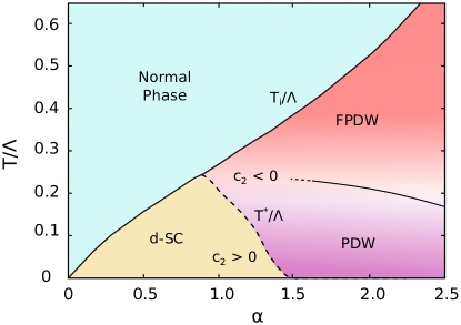
Our results are summarized in the phase diagram, Fig. 1. is the instability temperature of the homogeneous -wave state. The analysis of fluctuations allows us to define two different regimes. At weak coupling, , the uniform -wave paired state is the ground state; at larger (strong coupling), SC fluctuations at finite momentum lead to two modulated pairing phases – the PDW ground state and a higher temperature FPDW phase that condenses into a PDW ordered phase below a coherence temperature (). As expected in the BCS limit, the instability temperature and the coherence temperature coincide at weak coupling, while they decouple in the strong coupling regime where we find well formed pairs with no coherence. We do not perform here any calculation of the coherence temperature inside the modulated phase, however in analogy with results obtained for homogeneous -wave superconductors in the strong coupling limit Toschi et al. (2005) we anticipate for . The FPDW is found for temperature and it is characterized by pairs with finite momentum with no coherence. At , the ground state can be either the uniform -wave solution or the long-range PDW depending on the value of . Hence our model captures two key experimentally postulated modulated Cooper phases – a FPDW and a long-range PDW – in a single unified scheme.
The mechanism we present in this paper predicts spatially modulated pairing phases for , i.e. in strongly coupled electronic systems, with anisotropic interactions. Examples of low-density electronic materials include the Fe-based superconductor FeSe where quantum oscillations Terashima et al. (2014) as well as transport and scanning tunneling spectroscopy Kasahara et al. (2014a) show that both the electron and hole pockets are tiny with Fermi energies comparable or even smaller than the SC gap and for which we find several proposals of BCS-BEC cross-over physics in the literature Okazaki et al. (2014); Kasahara et al. (2014b); Watashige et al. (2017). Other “mixed-band” superconductors such as O vacancy- or Nb-doped SrTiO3 have one partially filled band with a large Fermi surface while the Fermi level intersects the other at or close to the band bottom Collignon et al. (2019). Even if these materials typically have more than one band close to or crossing the Fermi level, the results from our minimal model may eventually provide a suitable starting-point for the analysis of possible instabilities towards modulated pairing states in dilute multiorbital superconductors. Our results may also be relevant to the recent observation of superconductivity in twisted-bilayer graphene Cao et al. (2018) where interactions can be large compared to the bandwidth leading to large inter-particle distances Padhi et al. (2018) and hence possible strongly-coupled Cooper pairing.
The modulated phases we propose in this work, that include both the long-range ordered PDW as well as the FPDW at finite temperature, are distinct from earlier proposals in literature. Loder and coworkers Loder et al. (2010), considered similar models characterized by nearest neighbor attractive interaction with -wave symmetry and found Cooper pairing with finite center-of-mass momentum above a critical interaction strength. In Refs. Wårdh and Granath (2017); Wårdh et al. (2018), a modulated superconducting state is found in models which have correlated pair-hopping interactions. Other models that admit modulated SC ground states were proposed in the context of cold atoms Nikolić et al. (2010) where local interactions were considered in systems with multiple bands. Those references focused on the analysis of the long-range ordered state (mainly at zero temperature) without exploring the FPDW phase. The key contribution of our work is it provides an analytically tractable model where both fluctuating and long-range ordered PDWs can be explained under a single unified framework.
I Model
Let’s consider a single band SC system. The kinetic part of the Hamiltonian reads , where , is the chemical potential, the parabolic dispersion and we further assume . The pairing interaction is given by
| (1) |
is the constant SC coupling and is defined as
| (2) |
where is a form factor. In this work can be any anisotropic form factor; we consider, e.g. with -wave form. Our results do not depend qualitatively on the exact form of the anisotropy, provided it is strong enough, but they are distinct from the conventional -wave case . Here is the pairing energy scale.
We use the standard Hubbard-Stratonovich transformation to decouple the interaction term, Eq.1 and to derive the effective action in term of the bosonic pairing field (for a detailed derivation see Supplemental Material).
In standard BCS superconductors, the mean-field value of the pairing field is defined by minimizing the action with respect to the homogeneous value of and then solving this equation together with the one for the chemical potential. To study fluctuations of the pairing field around the mean-field value, we instead analyze the gaussian action obtained by retaining up to the second order in the fluctuating field with arbitrary momentum q given by
| (3) |
The static pairing susceptibility is explicitly given by , where the particle-particle propagator reads
| (4) |
with . Here is the temperature and the volume. Note that since , energies have dimensions of 2-D , and is therefore dimensionless.
The static susceptibility can be expanded in the hydrodynamic limit as
| (5) |
The instability temperature is defined as the highest temperature at which the susceptibility diverges, i.e. , as we assume that the minimum of the action, Eq. 17, is associated with the homogeneous order parameter. The coefficient provides instead information about the momentum rigidity of the fluctuating Cooper pairs i.e. the energy needed to move the center-of-mass momentum of the Cooper pairs from zero to a finite value. A negative momentum rigidity, , implies that finite momentum fluctuations can lower the energy of the system making the homogeneous SC solution unstable. This means that the highest temperature at which the pairing susceptibility, Eq. 5, diverges is actually associated to a critical mode with finite momentum.
In what follows we analyze the momentum-dependence of the static susceptibility, Eq. 5, looking for a sign change of the momentum rigidity parameter and using it as a proxy to identify possible spatially modulated SC regions in the phase diagram. It is worth noticing that is directly affected by the momentum properties of the pairing susceptibility i.e. the pairing symmetry. From Eq. 4, it is easy to verify that the anisotropy of the interactions affects the momentum dependence of the propagator not only in the SC phase via the symmetry of the SC order parameter, but also above the instability temperature where due to the overall form factor at the numerator. This reflects in a strong momentum dependence of the contributions to the rigidity parameter depending on the symmetry of the pairing interaction. We discuss below how this affects the development of critical finite-momentum fluctuations.
II Results and Discussion
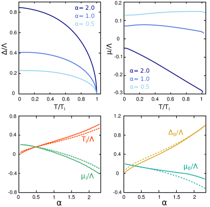
The mean-field analysis for the homogeneous -wave superconductor is shown in Fig.2. In panels (a)-(b) we report the self-consistent numerical mean-field solutions for the pairing function and the chemical potential as a function of temperature for three representative cases of the pairing strength , where for simplicity the weak-coupling expression is used at all . In panels (c)-(d) we show the same mean-field results at and as a function of . The change of sign of the chemical potential with increasing coupling strength is well-known from the BCS-BEC crossover problem Nozières and Schmitt-Rink (1985); Randeria and Taylor (2014); Duncan and Sá de Melo (2000); Benfatto et al. (2002); Chubukov et al. (2016). In the weak-coupling regime, the pairs are loosely bound and we recover the BCS expression . As the interaction increases, all fermions strongly bind in pairs and becomes negative and proportional to . In both the weak and strong coupling limits, the curves are similar to those derived for -wave superconductors in Chubukov et al. (2016), showing that the -wave symmetry of the pairing interaction does not affect the mean-field results qualitatively.
We first study the SC fluctuations above the instability temperature by analyze the static pairing susceptibility in the hydrodynamic limit, Eq. 5. The mass term is positive and vanishes as the temperature approaches the instability temperature as expected from a Ginzburg-Landau description of the transition.
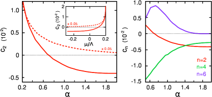
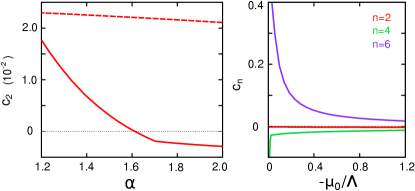
The analysis of the momentum rigidity of the fluctuating pairs above is shown in Fig. 3. The weak coupling region is characterized by a standard regime of fluctuations with . Here Cooper pairs with zero center-of-mass momentum are stable. Increasing , the momentum rigidity for the -wave pairing interaction (continuous line) monotonically decreases and becomes negative at intermediate coupling, , as shown in Fig. 3(a). This means that finite momentum critical fluctuations grow, increasing the coupling strength up to a critical value of the interaction for which the homogeneous SC solution can become unstable toward a modulated phase. Notice that becomes very small and eventually changes sign in the crossover between weak and strong coupling where also the chemical potential changes sign from positive to negative, see inset Fig. 3(a). The result changes qualitatively for the isotropic -wave interaction (dashed line) where the rigidity parameter decreases but remains positive even at strong coupling for the set of model parameter of our study swa .
To characterize the modulated SC state and check its stability, we expand the static susceptibility to higher order in momentum
| (6) |
We report the coefficients of the momentum expansion at in Fig. 3(b). Results are shown as a function of for the coupling regime in which . We need to expand the susceptibility up to find , since for our set of model parameters as in the conventional BCS case.
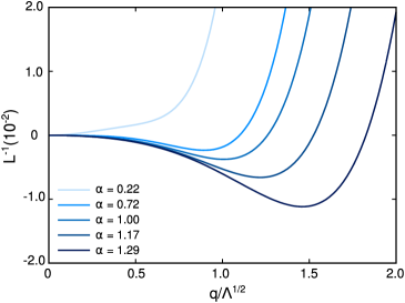
We analyze the momentum dependence of the static susceptibility at in Fig. 4, where we show the expansion of Eq. 20 up to sixth order for different values of . At the instability temperature, by definition and the minimum of the function is determined by the higher order coefficients. At weak coupling, where is large and positive, the minimum of is located at zero momentum. As the pairing interaction increases becomes small and eventually changes sign at . Here, since , the minimum shifts discontinuously to a finite momentum , i.e. by increasing the interactions the modulated phase emerges at via a first order transition from the homogeneous -wave SC solution, in analogy with the results found at in Loder et al. (2010); Wårdh and Granath (2017). The non-zero value of at signals the formation of the FPDW state with finite momentum pairing but no long range coherent order. Note that the finite order parameter jump is a non-universal quantity and depends on microscopic details of the chosen model, as is a feature of any generic first order transition. The momentum characterizing the modulated phase shifts toward larger values increasing the coupling parameters. In the strong coupling regime, , the minimum occurs at , (not shown), for this range of the interaction the analysis of the momentum characterizing the modulated phase requires the implementation of a non perturbative approach.
The sign change of the momentum rigidity parameter discussed at can be traced down in temperature (dashed line in Fig. 1). At the homogeneous -wave state becomes unstable, now toward a PDW, for a slightly higher value of the coupling where the chemical potential also changes sign (see Fig.2d). The stability of the PDW phase requires expanding up to the sixth-order, , as we show in the Supplementary Material.
The results of our numerical study are summarized in the phase diagram of Fig. 1. We characterized the SC region below by the sign of the momentum rigidity parameter (dashed line). The sign change of the coefficient at strong coupling signals the presence of critical SC fluctuations at finite momentum that make the -wave homogeneous state unstable toward either an FPDW or PDW. The pink and purple regions indicate the FPDW and the long-range ordered PDW state at high and low temperatures respectively. We leave for future work the explicit calculation of the coherence temperature below which the FPDW condenses. The color gradient indicates approximately the expected behaviour based on previous analysis of the coherence energy scale for the homogeneous -wave SC state Toschi et al. (2005).
Analytical calculations of the momentum rigidity can be easily performed within a simplified model in which the chemical potential is used as parameter. Both at and , we find qualitatively the same results discussed within the numerical study. In particular, within the analytical calculations sketched in the Supplementary Material, the momentum rigidity parameter follows the chemical potential behaviour, i.e. for . This relation is qualitatively in agreement with the numerical study performed computing self-consistently , as one can see from the inset of Fig. 3(a).
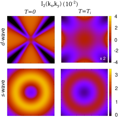
The strategy implemented here to investigate how finite momentum fluctuations become critical at strong coupling is based on the analysis of the momentum rigidity parameter. This method presents two main advantages with respect to other theoretical approaches. On the hand, as already discussed, it allows us to explore the finite temperature regime and analyze the FPDW state. On the other hand, it provides a physical understanding of the importance of the anisotropy of the pairing interactions in the development of the modulated phase. As one can see in Eq. 4, the symmetry of the pairing interactions dramatically affects the momentum dependence of the propagator not only in the SC phase, but also in the normal one when due to the overall form factor . This is reflected in a strong momentum dependence of the contribution to the momentum rigidity parameter. In fact, after performing analytically the Matsubara summation, the computation of the coefficient reduces to an integral over the Brillouin zone . The expression for is given in the Supplemental Material, but here we show here in Fig.5 2D maps of for both -wave and -wave at and . In the isotropic -wave case, the contributions to the momentum rigidity coming from different momenta, , are positive at any . On the other hand, in the -wave case the contributions to the momentum rigidity coming from the nodal regions are negative and dominate the overall sign of the coefficient.
III Conclusions
A consistent explanation for the occurrence of both static and fluctuating Cooper pairs with finite momentum in the phase diagram of materials such as cuprates has been a long-standing problem. This is primarily because an identification of the microscopic ingredients driving such exotic pairing has been elusive. The results in this paper point toward a simple and unified framework that naturally promotes both fluctuating and static pair-density wave (FPDW and PDW) phases over their zero momentum counterparts. Fig. 1 summarizes the main conclusions of our work, supported not only by numerical evaluations but also transparent analytical estimates (see Supplemental Material). The two key ingredients resulting in a high temperature FPDW and low temperature PDW phases are a) anisotropic (e.g. -wave) pair interactions and b) intermediate to strong coupling ratio of , where is the pair binding energy for two electrons on the Fermi surface in the presence of an attractive interaction, and is the Fermi energy. Well below a critical value of , only uniform zero momentum -wave pairing is favored. In the approximate range of , the FPDW phase, characterized by a negative momentum rigidity and positive (see Fig. 3), is stable over a range of temperatures below the instability temperature . However, in this range of a uniform -wave pair is still favored at zero temperature. For , the PDW phase is more stable than a uniform solution at and a finite momentum pair exists for all temperatures below . The modulation wave vector Q of the paired phases is determined by the ratio and acquires a jump with increasing as in a first order transition (see Fig. 4).
The FPDW and PDW phases are stabilized by contributions to the fluctuation free energy arising from momenta close to the nodal regions in the Brillouin zone. These contributions, which also should drive strong anisotropy in the phase stiffness near , are suppressed (enhanced) at weak (strong) coupling thus leading to a modulated phase above a critical pairing strength. This simplified picture is confirmed from our numerical calculations (Fig. 5). Finally, while our work primarily focuses on the instability temperature in the strong coupling limit, the behavior of the condensation temperature and the fluctuations around the PDW ground state in this setting are open problems that will require further investigations. Our work does not consider the competing effects of a nematic superconducting phase that has been phenomenologically found to suppress the PDW at in 2D Berg et al. (2009a); Barci and Fradkin (2011). In addition, even if allowed by our model, we have not addressed the possible coexistence at low of a PDW and a homogeneous -wave superconductor, as suggested by cuprate experiments Agterberg et al. (2019); Choubey et al. (2020). Our results as such set the stage for future microscopic descriptions of modulated superconductivity in strongly coupled materials.
IV Acknowledgements
We thank P. Abbamonte, B.M. Andersen, S. Caprara, A. Chubukov, E. Fradkin, S. A. Kivelson, M. Granath and A. Toschi for useful discussions and suggestions. L. F. acknowledges support by the European Union’s Horizon 2020 research and innovation programme through the Marie Sklodowska-Curie grant SuperCoop (Grant No 838526). This work is supported by the DOE grant number DE-FG02-05ER46236.
These authors contributed equally to this work.
csetty@rice.edu
laura.fanfarillo@ufl.edu
pjh@phys.ufl.edu
References
- Bardeen et al. (1957) J. Bardeen, L. N. Cooper, and J. R. Schrieffer, Phys. Rev. 108, 1175 (1957).
- Larkin and Varlamov (2005) A. Larkin and A. Varlamov, Theory of fluctuations in superconductors (Clarendon Press, 2005).
- Fulde and Ferrell (1964) P. Fulde and R. A. Ferrell, Physical Review 135, A550 (1964).
- Larkin and Ovchinnikov (1965) A. Larkin and Y. N. Ovchinnikov, JETP 20, 762 (1965).
- Agterberg et al. (2019) D. F. Agterberg, J. Davis, S. D. Edkins, E. Fradkin, D. J. Van Harlingen, P. A. Lee, L. Radzihovsky, J. M. Tranquada, Y. Wang, et al., arXiv preprint arXiv:1904.09687 (2019).
- Toschi et al. (2005) A. Toschi, M. Capone, and C. Castellani, Phys. Rev. B 72, 235118 (2005).
- Berg et al. (2007) E. Berg, E. Fradkin, E.-A. Kim, S. A. Kivelson, V. Oganesyan, J. M. Tranquada, and S. Zhang, Physical review letters 99, 127003 (2007).
- Berg et al. (2009a) E. Berg, E. Fradkin, and S. A. Kivelson, Nature Physics 5, 830 (2009a).
- Berg et al. (2009b) E. Berg, E. Fradkin, S. A. Kivelson, and J. M. Tranquada, New Journal of Physics 11, 115004 (2009b).
- Nikolić et al. (2010) P. Nikolić, A. A. Burkov, and A. Paramekanti, Physical Review B 81, 012504 (2010).
- Loder et al. (2010) F. Loder, A. P. Kampf, and T. Kopp, Physical Review B 81, 020511 (2010).
- Barci and Fradkin (2011) D. G. Barci and E. Fradkin, Physical Review B 83, 100509 (2011).
- Loder et al. (2011) F. Loder, S. Graser, A. P. Kampf, and T. Kopp, Physical review letters 107, 187001 (2011).
- Nikolić and Tešanović (2011) P. Nikolić and Z. Tešanović, Physical Review B 83, 064501 (2011).
- Jaefari and Fradkin (2012) A. Jaefari and E. Fradkin, Physical Review B 85, 035104 (2012).
- Lee (2014) P. A. Lee, Physical Review X 4, 031017 (2014).
- Soto-Garrido and Fradkin (2014) R. Soto-Garrido and E. Fradkin, Physical Review B 89, 165126 (2014).
- Soto-Garrido et al. (2015) R. Soto-Garrido, G. Y. Cho, and E. Fradkin, Physical Review B 91, 195102 (2015).
- Wårdh and Granath (2017) J. Wårdh and M. Granath, Physical Review B 96, 224503 (2017).
- Wårdh et al. (2018) J. Wårdh, B. M. Andersen, and M. Granath, Physical Review B 98, 224501 (2018).
- Himeda et al. (2002) A. Himeda, T. Kato, and M. Ogata, Physical review letters 88, 117001 (2002).
- Raczkowski et al. (2007) M. Raczkowski, M. Capello, D. Poilblanc, R. Frésard, and A. M. Oleś, Physical Review B 76, 140505 (2007).
- Capello et al. (2008) M. Capello, M. Raczkowski, and D. Poilblanc, Physical Review B 77, 224502 (2008).
- Yang et al. (2009) K.-Y. Yang, W. Q. Chen, T. M. Rice, M. Sigrist, and F.-C. Zhang, New Journal of Physics 11, 055053 (2009).
- Berg et al. (2010) E. Berg, E. Fradkin, and S. A. Kivelson, Physical review letters 105, 146403 (2010).
- Corboz et al. (2014) P. Corboz, T. M. Rice, and M. Troyer, Physical review letters 113, 046402 (2014).
- Choubey et al. (2020) P. Choubey, S. H. Joo, K. Fujita, Z. Du, S. D. Edkins, M. H. Hamidian, H. Eisaki, S. Uchida, A. P. Mackenzie, J. Lee, J. C. S. Davis, and P. J. Hirschfeld, Proceedings of the National Academy of Sciences 117, 14805 (2020), https://www.pnas.org/content/117/26/14805.full.pdf .
- Li et al. (2007) Q. Li, M. Hücker, G. Gu, A. Tsvelik, and J. Tranquada, Physical review letters 99, 067001 (2007).
- Tranquada et al. (2008) J. Tranquada, G. Gu, M. Hücker, Q. Jie, H.-J. Kang, R. Klingeler, Q. Li, N. Tristan, J. Wen, G. Xu, et al., Physical Review B 78, 174529 (2008).
- Schafgans et al. (2010a) A. Schafgans, A. LaForge, S. Dordevic, M. Qazilbash, W. Padilla, K. Burch, Z. Li, S. Komiya, Y. Ando, and D. Basov, Physical review letters 104, 157002 (2010a).
- Schafgans et al. (2010b) A. Schafgans, C. Homes, G. Gu, S. Komiya, Y. Ando, and D. Basov, Physical Review B 82, 100505 (2010b).
- Jacobsen et al. (2015) H. Jacobsen, I. Zaliznyak, A. Savici, B. Winn, S. Chang, M. Hücker, G. Gu, and J. Tranquada, Physical Review B 92, 174525 (2015).
- Hamidian et al. (2016) M. Hamidian, S. Edkins, S. H. Joo, A. Kostin, H. Eisaki, S. Uchida, M. Lawler, E.-A. Kim, A. Mackenzie, K. Fujita, et al., Nature 532, 343 (2016).
- Zhong et al. (2018) R. Zhong, J. Schneeloch, H. Chi, Q. Li, G. Gu, and J. Tranquada, Physical Review B 97, 134520 (2018).
- Rajasekaran et al. (2018) S. Rajasekaran, J.-i. Okamoto, L. Mathey, M. Fechner, V. Thampy, G. D. Gu, and A. Cavalleri, Science 359, 575 (2018).
- Edkins et al. (2019) S. D. Edkins, A. Kostin, K. Fujita, A. P. Mackenzie, H. Eisaki, S. Uchida, S. Sachdev, M. J. Lawler, E.-A. Kim, J. Séamus Davis, and M. H. Hamidian, Science 364, 976 (2019).
- Du et al. (2020) Z. Du, H. Li, S. H. Joo, E. P. Donoway, J. Lee, J. S. Davis, G. Gu, P. D. Johnson, and K. Fujita, Nature 580, 65 (2020).
- Wang et al. (2021) S. Wang, P. Choubey, Y. X. Chong, W. Chen, W. Ren, H. Eisaki, S. Uchida, P. J. Hirschfeld, and J. Séamus Davis, arXiv preprint arXiv:2105.06518 (2021).
- Kivelson et al. (2003) S. A. Kivelson, I. P. Bindloss, E. Fradkin, V. Oganesyan, J. Tranquada, A. Kapitulnik, and C. Howald, Reviews of Modern Physics 75, 1201 (2003).
- Terashima et al. (2014) T. Terashima, N. Kikugawa, A. Kiswandhi, E.-S. Choi, J. S. Brooks, S. Kasahara, T. Watashige, H. Ikeda, T. Shibauchi, Y. Matsuda, et al., Physical Review B 90, 144517 (2014).
- Kasahara et al. (2014a) S. Kasahara, T. Watashige, T. Hanaguri, Y. Kohsaka, T. Yamashita, Y. Shimoyama, Y. Mizukami, R. Endo, H. Ikeda, K. Aoyama, et al., Proceedings of the National Academy of Sciences 111, 16309 (2014a).
- Okazaki et al. (2014) K. Okazaki, Y. Ito, Y. Ota, Y. Kotani, T. Shimojima, T. Kiss, S. Watanabe, C.-T. Chen, S. Niitaka, T. Hanaguri, et al., Scientific reports 4, 1 (2014).
- Kasahara et al. (2014b) S. Kasahara, T. Watashige, T. Hanaguri, Y. Kohsaka, T. Yamashita, Y. Shimoyama, Y. Mizukami, R. Endo, H. Ikeda, K. Aoyama, et al., Proceedings of the National Academy of Sciences 111, 16309 (2014b).
- Watashige et al. (2017) T. Watashige, S. Arsenijević, T. Yamashita, D. Terazawa, T. Onishi, L. Opherden, S. Kasahara, Y. Tokiwa, Y. Kasahara, T. Shibauchi, et al., Journal of the Physical Society of Japan 86, 014707 (2017).
- Collignon et al. (2019) C. Collignon, X. Lin, C. W. Rischau, B. Fauqué, and K. Behnia, Annual Review of Condensed Matter Physics 10, 25 (2019), https://doi.org/10.1146/annurev-conmatphys-031218-013144 .
- Cao et al. (2018) Y. Cao, V. Fatemi, S. Fang, K. Watanabe, T. Taniguchi, E. Kaxiras, and P. Jarillo-Herrero, Nature 556, 43 (2018).
- Padhi et al. (2018) B. Padhi, C. Setty, and P. W. Phillips, Nano letters 18, 6175 (2018).
- Nozières and Schmitt-Rink (1985) P. Nozières and S. Schmitt-Rink, Journal of Low Temperature Physics 59, 195 (1985).
- Randeria and Taylor (2014) M. Randeria and E. Taylor, Annual Review of Condensed Matter Physics 5, 209 (2014), https://doi.org/10.1146/annurev-conmatphys-031113-133829 .
- Duncan and Sá de Melo (2000) R. D. Duncan and C. A. R. Sá de Melo, Phys. Rev. B 62, 9675 (2000).
- Benfatto et al. (2002) L. Benfatto, A. Toschi, S. Caprara, and C. Castellani, Phys. Rev. B 66, 054515 (2002).
- Chubukov et al. (2016) A. V. Chubukov, I. Eremin, and D. V. Efremov, Phys. Rev. B 93, 174516 (2016).
- (53) This result differs from the analysis of Benfatto et al. (2002), in which a sign change of the rigidity parameter is found for a SC system with -wave pairing symmetry at strong coupling. In this case, however, the authors first perform a strong coupling expansion of the pairing susceptibility and only subsequently expand the approximated result in powers of .
- Negele and Orland (1988) J. Negele and H. Orland, Quantum Many Particle System (Addison-Wesley, 1988).
V Supplemental Material
V.1 Derivation of the effective action for the fluctuating Cooper pairs
We consider a single band superconducting (SC) system, assuming a parabolic band dispersion where and is the chemical potential. The pairing interaction is given by
| (7) | |||||
| (8) |
is the constant SC coupling, is the angular factor defined as , with , where is the pairing energy cut-off.
We can decouple the interaction term using the standard Hubbard-Stratonovich transformation Negele and Orland (1988). The resulting action is given by
| (9) |
where is the Hubbard-Stratonovich field associated with and we put and . Introducing the Nambu spinor, we can rewrite the action as
| (10) |
with the matrix defined as
We can integrate out the fermions and separate . contains the contribution of the homogeneous and constant components of the Hubbard-Stratonovich field (i.e. ) while the contains the fluctuating part. Thus the action reads
| (11) | |||||
Here
| (12) |
with ; the fluctuation contributions of the pairing field is contained instead in
| (13) |
The saddle-point equation explicitly reads
| (14) |
evaluating the trace the above expression reduces to , i.e. explicitly
| (15) |
the usual BCS equation. Eq.(15) has to be solved self-consistently with the equation for the chemical potential
| (16) |
where we fix to the electronic density.
To analyze the fluctuations of SC field around the mean field solution, we expand up to second order in . The Gaussian action then reads
| (17) |
where is the particle-particle propagator
| (18) |
By expanding the Gaussian action at small frequency and momentum up to second order, we obtain the familiar expression
| (19) |
where is the mass term that vanishes at the instability temperature, is the stiffness that describes the momentum rigidity of the fluctuating Cooper pairs, and is the damping coefficient that at weak coupling reduces to the microscopic value of the Ginzburg-Landau damping , where is the density of states at the Fermi level Larkin and Varlamov (2005). As in this work we are interested in the analysis of static spatially modulated SC state, here on we focus on the momentum dependency only.
In the above treatment Eqs. (15)-(19), we implicitly assumed that the broken phase is a static homogeneous superconductor. i.e. we assumed that the minimum of the action is associated with the homogeneous and constant value of the order parameter , Eqs. (14) and (15). This implies that the highest temperature for which the pairing susceptibility diverges is determined by the mass term of Eq.(19). Notice, however that, if the highest temperature associated with the divergence of is found at for finite , this means that the instability is associated with a spatially non-uniform SC mode. If this is the case, it means that the finite momentum fluctuations are actually lowering the energy in Eq.(17).
In this work we use a perturbative approach to explore the possible emergence of a spatially modulated SC state from the homogeneous -wave superconductor. We study the momentum dependence of the static pairing susceptibility of the homogeneous -wave superconductor and look for a negative sign of the momentum rigidity parameter in Eq.(19). Notice that, in order to analyze the stability of the modulated SC phases, we will need to go beyond the second order in the momentum expansion
| (20) |
In the following we assume , as a consequence energies have dimensions of 2-D , and is therefore dimensionless.
V.2 Numerical Analysis
We analyze the mean-field solution at finite temperature as a function of the pairing strength . We explore the space of the parameters at low-density fixing the Fermi energy , where is the density of states at the Fermi level in 2D, and varying the superconducting coupling in Eq.(15). For simplicity we use the weak-coupling relation between the bound state energy and the SC coupling, i.e. . The mean field results for and as a function of temperature for different values of the pairing strength are shown in Fig.2 of the main text.
To study the fluctuations around the mean-field values of we analyze the static pairing susceptibility, , defined in Eqs. (17)-(18) by setting . Using the explicit expression for the normal and anomalous Green functions, Eq. (12), the pairing propagator reads
| (21) |
that can be evaluated at each temperature by using for and the mean-field values obtained solving Eqs. (15)-(16). After performing the Matsubara summation we can write the particle-particle propagator as
| (22) |
where we defined as
and is the Fermi function. To obtain the polynomial form discussed in Eq. (20), we expand the integrand around . We fix along , but the expansion along different q directions can generally yield quantitatively distinct results due to the anisotropy. Hereafter our derivatives are meant as . The mass terms is given by
| (24) |
while the higher order coefficients read
| (25) |
The momentum dependence of at and at is shown in Fig.5 of the main text where we report both the -wave and -wave case.
For the set of parameters used in this work we need to expand up to sixth order to check the stability of the finite momentum state. In Fig. 2 of the main text we show the behavior of , as a function of at . We use dimensionless units i.e. renormalized as . In Fig. 6, we report the results at . As one can see also at zero temperature we find a sign change of the momentum rigidity parameter at strong coupling where we also find and . The critical value of the interaction at which the rigidity vanishes is slightly larger than the one found at the instability temperature. Notice that in terms of we find again that the sign change of occur in the same range of interactions in which changes its value from positive to negative.
In addition to and , we numerically compute at finite temperature for to build the phase diagram in Fig.1 of the main text where we explicitly show the critical temperature along which the rigidity parameter vanishes.
V.3 Characterization of the modulated SC phase
We can derive information about the modulated SC phase analyzing the static susceptibility written as a sixth degree polynomial
| (26) |
where the odd terms vanish for symmetry. The extrema of occur at with
| (27) |
Let’s assume that the minima occur at finite momentum, in this case one can further expand the polynomial around Q so that we can find an approximate expression for the susceptibility of the modulated SC phase
| (28) |
with and the mass and the momentum rigidity associated with the modulated SC phase and defined in terms of the coefficients and the momentum characterizing the PDW phase as
It is worth noticing that by assuming for the mass term of the homogeneous state a standard Ginzburg-Landau temperature dependence , with , we can easily recover an analogous expression for
| (30) |
where . For the set of parameter used in this work we verify that when this correction is positive, i.e. the instability temperature associated with the PDW phase is higher than the one of the -wave homogeneous one.
Analogously one can verify that in the region of the phase diagram defined by the momentum rigidity parameter associated with the PDW state is now positive, meaning that the divergence of the susceptibility occurs at and is determined indeed by , while any momentum fluctuation around increases the energy of the system.
For example, given a pairing interaction , we find at that the critical fluctuations at finite momentum are characterized by a wave-vector and a positive momentum rigidity parameter . The correlation length can be derived from as . For the set of parameter used here we find that at is of the same order of magnitude of the length scale set by the energy cut-off of pairing, i.e. .
V.4 Analytical derivation of the sign change of the momentum rigidity parameter
In this work we analyze numerically the momentum dependence of the static pairing susceptibility, and show that for intermediate value of the interaction the SC fluctuations at finite momentum become critical. We use as a proxy the sign change of the momentum rigidity parameter that becomes negative at a critical interaction , whose exact value depends on temperature and system parameters. In this section, we derive an approximate formula that provides evidence of the sign change of the quadratic coefficient of the -wave SC susceptibility, although it gives a quantitatively imprecise value of the chemical potential where it actually occurs in the fully self-consistent evaluation.
We focus on the analysis of the SC fluctuation at the instability temperature, . The particle-particle propagator Eq. (18) in this case reads
| (31) |
and as we are interested in the static case we set .
The term of the SC susceptibility at reduces to
| (32) |
in agreement with Eqs. (21)-(24) once we set . By solving it together with
| (33) |
for the chemical potential at , we derive the expression for and . This yields for
| (34) | |||||
| (35) |
where is the chemical potential at . To obtain the contribution from terms, we need to evaluate :
To see that the sign change occurs for a negative , first set . We obtain
| (37) |
with . Note as . To obtain the opposite sign, the finiteness of has to be taken into account while allowing for the Matsubara frequency to be large. An approximate trend with can be obtained as
Hence there must be a critical value of the chemical potential for which the coefficient must change sign. This is given for finite and as
| (39) |
where is the first derivative of the digamma function, and . Note the order in which and go to infinity matters. That is, for before . Otherwise, we see that . Hence the presence of a lattice is an important ingredient in the problem.
An analogous conclusion can be arrived at zero temperature with an anisotropic -wave gap function. The expansion is already tedious at second order but can nevertheless be evaluated as a function of the chemical potential. A similar sign change of occurs at a critical value of the zero temperature . The full self-consistent calculation has been performed via numerical analysis and it is shown in the main text.