DAMIC Collaboration
Characterization of the background spectrum in DAMIC at SNOLAB
Abstract
We construct the first comprehensive radioactive background model for a dark matter search with charge-coupled devices (CCDs). We leverage the well-characterized depth and energy resolution of the DAMIC at SNOLAB detector and a detailed GEANT4-based particle-transport simulation to model both bulk and surface backgrounds from natural radioactivity down to 50 eV. We fit to the energy and depth distributions of the observed ionization events to differentiate and constrain possible background sources, for example, bulk 3H from silicon cosmogenic activation and surface 210Pb from radon plate-out. We observe the bulk background rate of the DAMIC at SNOLAB CCDs to be as low as counts kg-1 day-1 keV, making it the most sensitive silicon dark matter detector. Finally, we discuss the properties of a statistically significant excess of events over the background model with energies below 200 eV.
I Introduction
The particle nature of dark matter is one of the most elusive mysteries in physics Kolb and Turner (1990); Bertone and Hooper (2018). After decades of searching for “heavy” weakly interacting massive particles (WIMPs) with masses 10– GeV/ Goodman and Witten (1985); Lewin and Smith (1996), all potential signals have so far been excluded or remain unverified. This effort has required unprecedented understanding of radioactive background sources down to the keV energy scale Schumann (2019). In the absence of a detection of the heavy WIMP, many experiments are refocusing on the possibility of lower mass dark matter particles that would produce energy signals below 1 keV Battaglieri et al. (2017). Such dark matter models are theoretically well-motivated but largely unexplored hypotheses that include low-mass WIMPs Zurek (2014), hidden-sector particles Hochberg et al. (2017); Essig et al. (2012), axions and axion-like particles Graham et al. (2015), and strongly interacting massive particles (SIMPs) Davis (2017); Collar (2018), among many others. A review of simplified models for low-mass dark matter can be found in Ref. Lin (2019).
A dominant method of searching for lower mass dark matter is to use detectors that measure the small ionization signals produced from a dark matter particle recoiling off of either the nuclei or electrons in a material. This technique has been demonstrated by cryogenic detectors Amaral et al. (2020); Arnaud et al. (2020), noble liquid time-projection chambers Agnes et al. (2018); Aprile et al. (2019), and gaseous detectors Arnaud et al. (2018), to name a few. Here, we will focus on the use of charge-coupled devices (CCDs) by the Dark Matter In CCDs (DAMIC) experiment at SNOLAB to search for ionization produced by dark matter scattering in silicon. More specifically, we will detail the construction of the first comprehensive radioactive background model for a CCD detector down to a threshold of 50 eV (electron-equivalent energy available as ionization), which was recently used to set limits on GeV-scale WIMPs coupling to nuclei Aguilar-Arevalo et al. (2020). In Ref. Aguilar-Arevalo et al. (2020), we also reported an unexpected excess of events above the background model with energies eVee. This paper revisits the same data and provides supplementary information for a robust exploration of the reported event excess.
This paper is organized as follows. In Section II, we summarize our experimental setup, including a detailed description of the DAMIC at SNOLAB detector, CCD sensor operation, and our data analysis. In Section III, we expand on this discussion with a focus on backgrounds, as from radiocontaminants in detector materials and on their surfaces. We detail our application of the GEANT4 simulation package Allison et al. (2016) to these background sources and our modeling of the partial charge collection region discovered near the back surface of the CCDs. In Section IV, we present the construction of our radioactive background model from a fit to data above 6 keVee with templates constructed from simulated events, as well as an independent cross-check on the activity of surface 210Pb and the extrapolation of this model into our WIMP-search region. In Section V, we revisit our “WIMP search,” explore the event excess over the background model, and discuss its significance relative to our background model uncertainties. Finally, in Section VI, we summarize the results of this analysis and discuss future improvements and applications.
II Experimental Setup
DAMIC at SNOLAB is the first dark matter detector to employ a multi-CCD array. Following its original deployment Aguilar-Arevalo et al. (2016), it was upgraded for lower backgrounds, more CCD detectors, and longer exposure. The results of the latest detector installation include the search for hidden-sector dark matter particles from its interactions with electrons Aguilar-Arevalo et al. (2019a) and the most sensitive search for silicon nuclear recoils from the scattering of WIMPs with masses below 10 GeV Aguilar-Arevalo et al. (2020). Here, we describe in detail the DAMIC at SNOLAB detector, including CCD operation and data analysis.
II.1 DAMIC Detector
The DAMIC detector at SNOLAB consists of an array of eight CCD modules in a tower-like configuration that was installed in January 2017. The topmost CCD module (CCD 1) was fabricated with ultra-low radioactivity copper and is shielded from the others by ultra-low radioactivity lead. One of the other eight CCDs was disconnected soon after installation due to luminescence from one of the amplifiers, which produced unwanted charge throughout the CCD array. Of the remaining devices (CCDs 1–7), one device (CCD 2) was initially not operational but unexpectedly came back online after a temperature cycle and electronics restart caused by an unplanned power outage at SNOLAB in April 2017.
The DAMIC at SNOLAB CCDs were packaged by Fermi National Accelerator Laboratory (Fermilab). The CCD package consists of the CCD sensor and Kapton flex cable glued onto a silicon support frame cut from high-resistivity silicon wafers from Topsil (of the same origin as those used for CCD fabrication). The Kapton flex, fabricated by Cordova Printed Circuits Inc., was first glued using pressure-sensitive adhesive ARclad IS-7876, after which the sensor was glued using epoxy Epotek 301-2 and cured for two days in a laminar flow cabinet. A fully automatic Fine Wire Wedge Bonder was used to connect with aluminum wires the pads on the CCD to the corresponding pads on the flex cable. The flex cable has a miniature AirBorn connector installed on its end, which carries the signals to drive and read the CCD.
Each CCD module consists of a CCD package installed in a copper support frame. The modules slide into slots of a copper box Chavarria (2020) with wall thickness of 6.35 mm, which, in addition to mechanical support, acts as a cold IR (infrared radiation) shield during operation. Copper trays also slide into slots of the box to make the shelves that hold two 2.5 cm thick ancient lead (smelted years ago) bricks above and below CCD 1. The copper frame for CCD 1, the copper tray that holds the top ancient lead brick, and an additional mm thick copper plate placed on top of the lower ancient lead brick were made from high-purity copper electroformed by Pacific Northwest National Laboratory (PNNL) Hoppe et al. (2014).
All other copper parts of the CCD modules and box were machined using propylene glycol as lubricant at The University of Chicago from oxygen-free high conductivity (OFHC) Copper Alloy 10100 procured from Southern Copper & Supply Company. At least 3 mm of copper was removed from all surfaces of the stock plates when machining to minimize possible contamination introduced in the copper when it was rolled into plates. The machined copper parts and brass fasteners used for their assembly were cleaned and passivated with ultra-pure (Fisher Scientific Optima grade or equivalent) water and acids following the procedure from Ref. Hoppe et al. (2007). The packaged CCDs and modules were transported to SNOLAB by car and taken underground to be installed in the detector.
The copper box is suspended below an 18 cm high lead shield inside a 20 cm diameter, 79 cm long cylindrical copper cryostat. The cryostat is held at pressures of 10-6 mbar (10-4 Pa) by a HiCube 80 Eco turbomolecular pump. The internal cylindrical lead shield has a central 3.15 cm diameter hole to accommodate a concentric copper cold finger that makes thermal contact between the top of the copper box and a Cryomech AL63 cold head above the shield. A temperature sensor and a heater installed at the interface between the cold head and the cold finger are connected to a LakeShore 335 unit to control the temperature of the system. The Kapton flex cables run along the side of the lead shield through an outer channel before they connect to a second-stage Kapton flex extension that includes an amplifier for the CCD output signal. The flex extensions connect to the vacuum-side of a vacuum interface board (VIB) that acts as the electronics feedthrough.
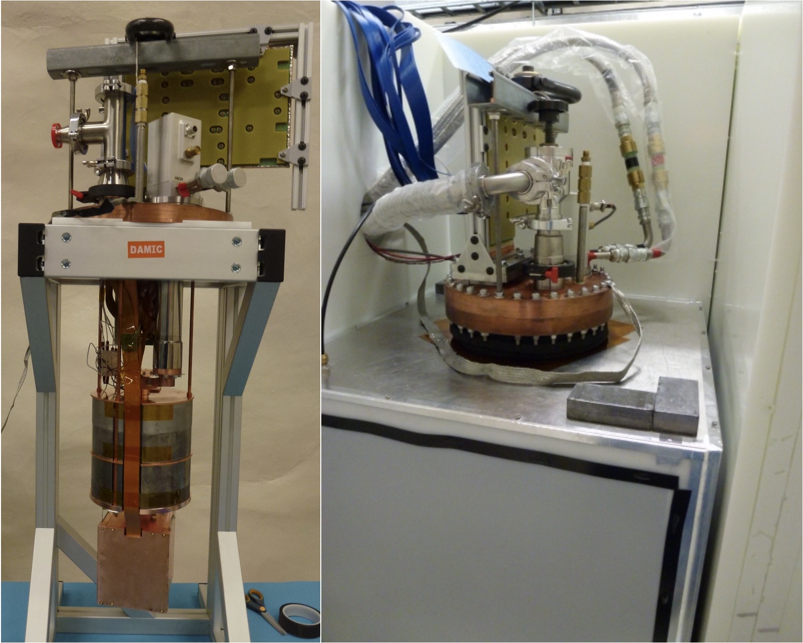
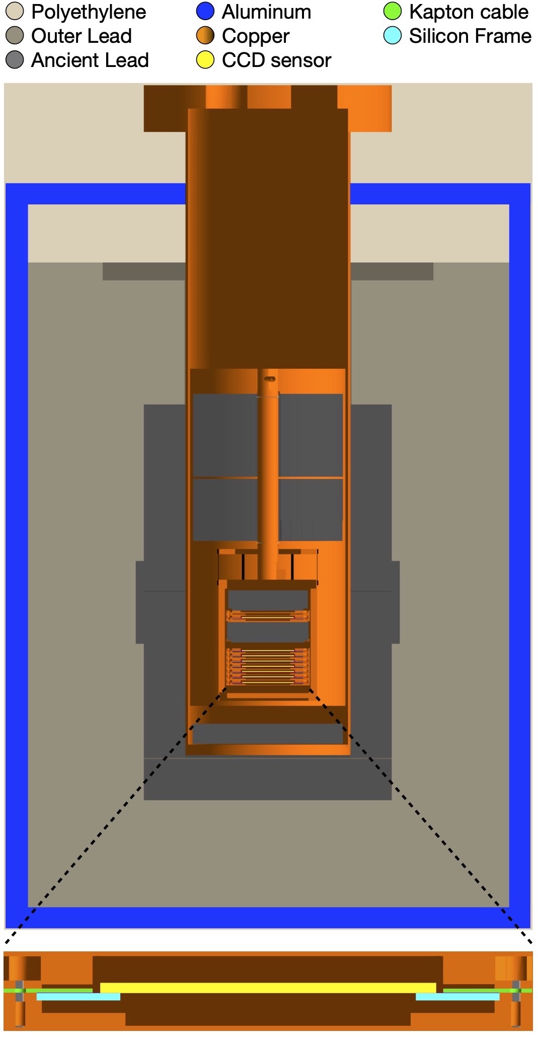
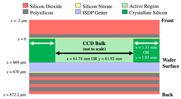
The copper cryostat is lowered into a cylindrical hole in a rectangular lead castle with its flange remaining above the lead so that the ports are accessible. In this configuration, the CCDs are shielded by at least 20 cm of lead in all directions, with the innermost 5 cm being ancient lead, and the outer lead being low-radioactivity lead from the Doe Run Company Leonard et al. (2008). All ancient lead surfaces were cleaned in an ultra-pure dilute nitric acid bath Abgrall et al. (2016). A hermetic box covers the lead castle and seals around the neck of the cryostat. Nitrogen gas with a flow rate of 2 L/min is used to keep the volume inside this box (around the cryostat) filled with pure nitrogen slightly above atmospheric pressure and free from radon. Photographs of the detector are shown in Fig. 1 and a diagram of a cross-section of the geometry is shown in Fig. 2.
Around the lead castle and above the cryostat flange, 42 cm of high-density polyethylene shields against external neutrons. A horizontal access hole through the polyethylene feeds through the pumping line, the helium lines from the outside compressor to the cold head, the boiloff nitrogen from a liquid-nitrogen dewar, and electrical cables. Blue coaxial cables connect the air-side of the VIB to the CCD controller, the Monsoon system developed for the Dark Energy Camera Mclean et al. (2012); Flaugher et al. (2015), that is located outside the shield. The Monsoon sends the clock signals and biases to the CCDs, and processes the analog CCD signal. The Monsoon is programmed by a DAQ computer that receives the measured pixel values via optical fiber.
II.2 Charge-Coupled Devices
DAMIC CCDs were developed by Lawrence Berkeley National Laboratory (LBNL) MicroSystems Lab Holland et al. (2003) and consist of a m-thick substrate of n-type high-resistivity (10 k cm) silicon with a buried p-channel and an array of pixels on the front surface for charge collection and transfer. Each pixel is 15 15 m2 in area and consists of a three-phase polysilicon gate structure. The CCDs feature a 1 m thick in-situ doped polysilicon (ISDP) backside gettering layer that absorbs heavy metals and other impurities from the silicon substrate during manufacturing and acts as the backside contact to fully deplete the device during operation Holland (1989); Lecrosnier et al. (1980). The overall thickness of a CCD is estimated from the fabrication process flow to be m, with an active thickness of m and m-thick dead layers on the front and back surfaces. Considering the pixel array area of 62 62 mm2, the total active mass of each CCD is 6.0 g.
A substrate bias of 70 V creates an electric field across the fully-depleted silicon bulk, in what we will refer to as the -direction. A nuclear or electronic recoil in the silicon will ionize silicon atoms and produce electron-hole (e-h) pairs over the band gap of 1.12 eV Alex et al. (1996). Charges are drifted by the electric field, and holes are collected in the potential minimum below the polysilicon gates, where they are stored for the duration of an exposure. Clocking the three-phase gate potentials allows efficient transfer of charges across the CCD in the -direction and into the serial register (last row). Channel stops formed by ion implantation prevent movement of charge in the -direction (across columns) in the main pixel array. Clocking the gate potentials in the serial register shifts charges in the -direction and into the “sense” node, where the pixel charge is measured. Charge transfer inefficiencies (i.e., fraction of the charge left behind after every pixel transfer) in LBNL CCDs are typically Holland et al. (2003).
Two MOSFET readout amplifiers are located at opposite ends of the serial register, one of which is used to read out the transferred charge and the other to simultaneously read empty mirror pixels (as charges are always clocked in the same -direction). The pixel charge is estimated with the correlated double sampling (CDS) technique Janesick (2001). First, any residual charge in the low-capacitance sense node is cleared with a reset pulse. A reference value for the sense node is then obtained by integrating its potential over 40 s. The pixel charge is then transferred to the sense node and its potential measured again over the same integration time. The difference between the two measured values is then proportional to the pixel charge. After the two measurements, the pixel charge is discarded with a reset pulse and the procedure is repeated with the next pixel. The CDS technique has been previously demonstrated in DAMIC CCDs to have an uncertainty in the measurement of the pixel charge as low as 1.6 Aguilar-Arevalo et al. (2019a) once its integration time is optimized to suppress high-frequency noise. In the DAMIC electronics, the CDS operation is performed with an analog circuit whose output is sampled once per pixel by a 16-bit digitizer. From the sequence of digitized values, we construct an image whose pixel values above the digitizer baseline are proportional to the charge collected in the CCD pixel array.
For this analysis, we used a subset of DAMIC data where a variable in the readout software was modified so that 100 rows of the CCD pixel array were transferred into the serial register before the serial register was clocked and the pixel charge measured (referred to as 1x100 readout mode). This downsampling procedure at the readout stage results in an effective pixel size of 15 1500 m2. This procedure reduces the position resolution in the -direction but allows the charge from an ionization event (spread out over multiple rows) to be read out in a smaller number of measurements, substantially reducing the uncertainty in the total ionization charge (energy) from an interaction. With 1x100 readout, only a few percent of low-energy events populate more than one row in an image, which simplifies the analysis to one dimension (along rows), while retaining some coarse resolution in to study the spatial distribution of observed events.
When ionization is first produced in the CCD bulk, it drifts in the electric field, and experiences stochastic thermal motion that leads to diffusion, which results in an increase in the lateral spread of charges on the pixel array. For a point-like interaction in the active region of the CCD, diffusion leads to a Gaussian distribution of charge with spatial variance that is proportional to the carrier transit time and, hence, positively correlated with the depth of the interaction. Because we use data from 1x100 readout mode in this analysis, the clusters are collapsed along the dimension and only the lateral spread in can be measured. Thus, we rely on to reconstruct the depth of an event below the gates (defined as ). In general, diffusion can be modeled as Aguilar-Arevalo et al. (2016); Holland et al. (2003)
| (1) |
where the two parameters and are defined in the model as
| (2) |
Here, GeV-1 fm-1 is the permittivity of silicon at the operating temperature K Krupka et al. (2006), cm-3 is the nominal donor charge density Holland et al. (2003), is the Boltzmann constant, is the charge of an electron, V is the potential difference between the charge-collection well and the CCD backside111This differs from the substrate bias (70 V) since the potential minimum at the charge-collection well is V below ground Holland et al. (2003)., and m is the thickness of the CCD active region.
We use data taken with the DAMIC CCDs above ground at Fermilab (before deployment at SNOLAB) to extract the diffusion parameters. These data were acquired with the same electronics as in SNOLAB and in 1x1 readout mode to maximize spatial resolution. Surface laboratory images have a substantial background from muons, which deposit their energy in straight trajectories through the silicon bulk. From the (,) coordinates of the end points of an ionization track in an image, i.e., where the muon crosses the front () and the back () of the active region, we can reconstruct the coordinate at every point along the track. We perform a fit to the charge distribution of the observed muon tracks by maximizing
| (3) |
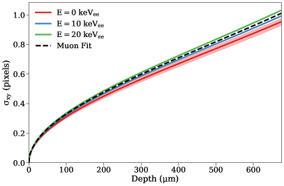
where is the probability of measuring charge for the pixel out of from a muon track constructed from trajectory convolved with a Gaussian charge spread as a function of depth using Eq. (1). From fits to a series of muon tracks, we obtain diffusion parameter values and , which are of the same order of magnitude as the theoretical calculations in Eq. (2). In our 1x100 data taken at SNOLAB, we observe a percent-level deviation from this calibration that is proportional to the event energy . To correct for this dependence, we fit to a linear function the maximum observed spread of data clusters as a function of energy in 0.5 keVee slices between 2–14 keVee. We find that in the SNOLAB data is well-described after a multiplicative linear correction to Eq. (1) of ( keVee). The final calibrated diffusion model is shown in Fig. 3.
II.3 Data Taking and Analysis
Since its initial installation in January 2017, the DAMIC detector acquired data almost continuously until September 2019 when the cryocooler failed. From January to September 2017, data was taken in 1x1 readout mode dedicated to searches for particles and decay sequences to determine the radioactive background sources in the detector (see Ref. Aguilar-Arevalo et al. (2021)). Following a LED calibration campaign in the summer of 2017, from September 2017 to December 2018, we accumulated all data used for both the construction of the background model and the WIMP search; these data were taken in 1x100 readout mode with either 100 ks ( hr) or 30 ks ( hr) exposures, where each exposure results in seven images (one per CCD). The temperature of the CCDs (150K in the 1x1 data) was decreased with time to reduce dark current: down to 140K for the first two-thirds of the 1x100 data used in this analysis, and further to 135K for the remaining third. We were cautious with lowering the temperature because temperature-induced mechanical stresses are a known cause of amplifier luminescence.
The 1x100 images acquired at SNOLAB are 4116 columns 42 rows. The first step in image processing is the removal of the image pedestal introduced by the digitizer baseline. The image pedestal is estimated to be ADU (analog-to-digital units) from the median value of every column and then subtracted from every pixel in the column. The same procedure was repeated in row segments of 1029 pixels across the entire image to remove any residual pedestal trend in the -direction. Noise picked up by the electronics chain of the system (e.g., by the cabling) is correlated between all CCD amplifier signals. We suppress from each pixel the correlated noise by subtracting the weighted sum of the corresponding pixel in the mirror images from all CCDs with the weights evaluated to minimize the pixel variance. After this procedure, the per-pixel noise is 1.6 ( eVee) Aguilar-Arevalo et al. (2019b), where we calibrate the pixel value to collected charge using an LED installed inside the DAMIC cryostat by following the calibration procedure with optical photons detailed in Ref. Aguilar-Arevalo et al. (2016). LED studies also demonstrate the linearity of the CCD energy scale to be within 5% down to 10 ( eVee) and confirm that the trailing charge after clocking the entire length of the serial register (4116 transfers) is 1%. To translate between the collected charge and electron-equivalent energy we use 3.8 eVee/ from Ref. Rodrigues et al. (2021) for the average kinetic energy deposited by a fast electron to ionize an e-h pair in silicon at the operating temperature of 140 K. We refine the calibration of the electron-equivalent energy scale by fitting to known lines in the data from 210Pb X-rays (10.8, 12.7, and 13.0 keV) and copper fluorescence (8.0 keV) for each individual CCD. We obtain an average gain of eV ADU-1. Given the 16 bit dynamic range of the digitizer, this results in a (CCD-dependent) pixel saturation value of keV. This calibration is in good agreement with similar CCDs calibrated on the surface with in-situ gamma and X-ray sources Ramanathan et al. (2017).
Data selection based on the quality of the images is made upon experimental criteria. The process starts with a visual inspection by the on-shift scientist during data taking, who flags any image with visible noise patterns for removal. DAMIC data is divided into stable acquisition “data runs” in between temperature changes or restart of the electronics, which were mostly caused by power outages at SNOLAB. Images at the beginning of each data run exhibit transients of high leakage current and are excluded. Following this removal of bad exposures, the ostensibly “good” data set consists of 864 exposures that result in 6048 images. We monitor radon levels around the DAMIC cryostat inside of the shield using a Rad7 monitor, and exclude periods when the average reading is above 5 Bq/m3, excluding 63 exposures (441 images). An additional set of 29 images across the 7 CCDs are removed as they show pixels with highly negative values (). Following image selection, the cumulative detector live time (per CCD) is 307 days. Furthermore, we remove regions at the edge of the images by accepting the central region 1283978 (5.78 cm in ) and by excluding rows and 42, leaving 6.0 cm in . This edge cut removes 7 of pixels, which results in a reduced CCD target mass of 5.6 g.
Regions of spatially localized leakage current (as from lattice defects) that may mimic ionization events are excluded based on the procedure described in Ref. Aguilar-Arevalo et al. (2016), in which maps of such areas are stored as masks that track individual pixels to be removed from consideration. Masks are generated for every CCD in every data run based on the procedure described in Ref. Aguilar-Arevalo et al. (2016). We calculate the median and median absolute deviation (MAD) of every pixel over all images in the data run and include in the mask pixels that either deviate more than three MAD from the median in at least 50 of the images or whose median or MAD is an outlier (). Masks from 35 data runs are combined to generate a single “iron mask” per CCD. The data runs considered consist of those used for this analysis and higher-temperature data runs acquired at 150 K and 170 K, which are more sensitive in identifying defects because of the strong dependence of leakage current on temperature Janesick (2001). For the 150 K data runs, acquired in 1x1 readout mode, we rebin the masks into 1x100 format. The “iron mask” for each CCD is approximately the union of the masks from all data runs, except for isolated pixels that are only found in masks from a small number of data runs, consistent with statistical fluctuations in the pixel values. Averaging over all CCDs, the “iron mask” removes 6.5 of pixels (keeping 93.5 of the average CCD mass).
We run clustering algorithms in unmasked regions of the images to identify charge spread over multiple pixels that originates from the same ionizing particle event. We apply two methods to cluster events, which we refer to as “fast clustering” and “likelihood clustering” and which are used in the background model construction (Section IV.1) and the WIMP search (Section V), respectively.
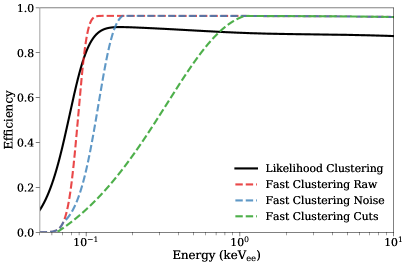
The “fast clustering” algorithm identifies contiguous groups of pixels each with signal larger than 4 ( 24 eVee). This algorithm effectively clusters all types of ionization events (point-like low energy depositions, high-energy electrons, muon tracks, alpha particles, etc.) regardless of the pattern on the pixel array. Because the fast clustering algorithm considers only pixels that contain charge, it can be used to efficiently translate many terabytes of simulated energy depositions into reconstructed coordinates without the need of a complete image simulation. If the sum of the pixel values in the cluster is 100 keVee, we perform a 2D Gaussian fit to the pixel values to obtain the energy and of the event. We select events that do not contain and are not touching a masked pixel. We require that the integral of the best-fit Gaussian gives the same energy as the sum of pixel values to within 5, and that the fit converges with a minimum negative log-likelihood value that is consistent with other clusters of similar energy. Figure 4 shows the efficiency of the fast clustering algorithm for simulated events where the charge is distributed in an empty pixel array (raw), an array containing simulated readout noise, and on the same array after applying the quality cuts mentioned here, which cause the efficiency to decrease rapidly for clusters with energies 1 keVee.
Conversely, the “likelihood clustering” algorithm is used to scan over a full image and calculate the likelihood of an energy deposition present in a window of predefined size. This algorithm only works for energies below 10 keVee, where an energy deposition can reasonably be considered point-like (much smaller than the pixel size) prior to diffusion. Before running likelihood clustering on every image, in addition to the iron mask, we mask any pixels that are part of clusters found by the fast clustering algorithm with energies above keVee, along with any pixels less than 200 pixels from the cluster in the -direction to avoid any low-energy events from charge transfer inefficiencies across the serial register. The algorithm is then used to iterate across the image row-by-row, calculating for each row segment (of variable but minimum width of 5 pixels) the likelihood that the pixel values can be described by white noise or white noise plus a Gaussian distribution of charge . When the negative log-likelihood of their ratio,
| (4) |
is sufficiently negative, a cluster is identified. Most clusters identified in this way have a small negative and can be attributed to noise.

We produce simulated images starting from blank (zero exposure) images, which are acquired immediately after each exposed image so that they almost only contain the readout noise of the detector. We then introduce shot noise uniformly in space to simulate the effect of leakage current. The good agreement between the measured and simulated distributions at low negative in Fig. 5 confirms that our modeling of noise clusters is accurate. To exclude such events from the WIMP search, we fit the simulated distribution with an exponential function and set a value of to ensure that there are fewer than 0.1 noise events expected in our dataset. This selection leads to a reconstruction efficiency below 50 eVee, which we set as our analysis threshold. In addition, we apply the following quality criteria: we remove clusters containing or adjacent to a masked pixel, clusters that span more than one row, clusters too close to each other on an image such that their fitting windows overlap, and clusters where the maximum pixel contains less than 20 of the total charge (indicating a charge distribution that is too broad to arise from a point-like event). The efficiency of these cuts is shown in Fig. 4 and is found to plateau around 90 above 120 eVee. The lower plateau value for the likelihood clustering compared to the fast clustering algorithm is because we consider clusters removed by the mask as an inefficiency in the likelihood clustering; since the simulation of events from fast clustering does not use blank CCD images, the CCD mask does not need to be applied.
III Background Sources and Detector Modeling
As with all dark matter detectors, it is critical to examine all possible sources of background events in DAMIC at SNOLAB. These backgrounds are primarily radiogenic and come from radiochemical impurities in and activation of detector materials, contamination deposited on detector surfaces, and external sources. For an accurate estimate of the different background contributions in our detector, we simulate radioactive backgrounds with the GEANT4 package, and include the effect of the partial charge collection region in the back of our sensors.
III.1 Material Assays
All materials used in the construction of DAMIC at SNOLAB were carefully catalogued and assayed for long-lived radioactivity. These assays focused primarily on the primordial 238U and 232Th chains, but also measured 40K in the detector materials. For the 238U chain, we consider the possibility that two different segments of this chain, delimited by 226Ra ( kyr) and 210Pb ( yr), may be out of secular equilibrium with 238U and with each other. A full list of the assay results of the materials used in the DAMIC at SNOLAB detector can be found in Table 1, and are detailed below.
| 238U | 226Ra | 210Pb | 232Th | 40K | 32Si | |
|---|---|---|---|---|---|---|
| CCD / Si frame | 11 Aguilar-Arevalo et al. (2021) | 5.3 Aguilar-Arevalo et al. (2021) | 160* Aguilar-Arevalo et al. (2021) | 7.3 Aguilar-Arevalo et al. (2021) | 0.5 [M] | Aguilar-Arevalo et al. (2021) |
| Kapton Cable | 58000 5000 [M] | 4900 5700 [G] | not measured | 3200 500 [M] | 29000 2000 [M] | N/A |
| OFHC Copper | 120 [M] | 130 [G] | 27000 8000 Abe et al. (2018) | 41 [M] | 31 [M] | N/A |
| Module Screws | 16000 44000 [G] | 138 [G] | 27000 8000† | 2300 1600 [G] | 28000 15000 [G] | N/A |
| Ancient Lead | 23 Orrell et al. (2016) | 260 [G] | Orrell et al. (2016) | Orrell et al. (2016) | 5.8 [M] | N/A |
| Outer Lead | 13 Leonard et al. (2008) | 200 [G] | () Leonard et al. (2008) | 4.6 Leonard et al. (2008) | 220 Leonard et al. (2008) | N/A |
For many of the materials, assays were performed using either Inductively-Coupled Mass Spectrometry (ICP-MS) or Glow Discharge Mass Spectrometry (GDMS). These techniques measure the elemental composition of a sample and estimate the activity of a specific isotope from its natural abundance. We adopt the standard values 1 Bq/kg 238U per 81 ppb U, 1 Bq/kg 232Th per 246 ppb Th, and 1 Bq/kg 40K per 32.3 ppm K Loach et al. (2016). All materials constrained by mass spectrometry are indicated as such in Table 1 with a superscript .
Most materials used in the DAMIC at SNOLAB detector were screened by Germanium -ray spectrometry at the SNOLAB -ray counting facility Lawson (2020). This method non-destructively measures the isotopic abundance from the intensity of specific lines from radioactive decays in the sample. All materials best-constrained by -ray counting are indicated in Table 1 with a superscript . A special case is the Epotek 301-2 used to glue the CCD to its silicon frame, which was activated with neutrons from the nuclear research reactor at North Carolina State University before performing ray spectroscopy of the activation products to estimate the abundance of the radiocontaminants initially present in the sample, a method known as Neutron Activation Analysis. The resulting measurement is below detectable limits and so the epoxy is omitted from this analysis; we place upper limits on Epotek 301-2 of , , and Bq/kg for 238U, 232Th, and 40K respectively, making this a suitable epoxy for future low radioactivity applications.
Some materials are best constrained by measurements published elsewhere. For example, the ancient lead used in the inner shield and around CCD 1 is from the same batch as the “U. Chicago Spanish lead” sample in Ref. Orrell et al. (2016). We thus use this measurement to constrain the bulk 210Pb content of our ancient lead. Similarly, the XMASS Collaboration has presented a robust analysis of the variation of bulk 210Pb content in commercially available OFHC copper Abe et al. (2018). While this is not a direct measurement of our copper, it provides an excellent starting point for our analysis. The PNNL electroformed copper (EFCu) used to house CCD 1 is far cleaner than the other materials of the detector Arnquist et al. (2020) and as such is treated as perfectly radiopure. Finally, the low-activity lead used in the outer DAMIC shield is of the same origin as the lead assayed by the EXO Collaboration Leonard et al. (2008). We use the EXO measurements to confirm the negligible contribution this lead has on our background model.
While we have performed some direct assays of our CCD silicon, only the 40K estimate from Secondary Ion Mass Spectrometry (SIMS) is better than the constraints that we can place with the CCDs themselves. The CCD analysis, originally demonstrated in Ref. Aguilar-Arevalo et al. (2015) and recently updated in Ref. Aguilar-Arevalo et al. (2021), provides better numbers for many of the long-lived isotopes in our detector by leveraging spatially coincident events from the same decay chain occurring over long timescales.
III.2 Material Activation
In addition to these measured radioisotopes, we take into account the cosmogenic activation of the detector materials before they are taken underground to SNOLAB. Activation of a material happens when high-energy cosmogenic neutrons cause spallation of material nuclei Cebrián (2017). Here we consider only activation of the silicon CCDs and copper parts, including the Kapton readout cables, which are 70 copper by mass.
For copper activation, we consider the average activity of an isotope during the WIMP search exposure to be
| (5) |
where the decay constant of the isotope is related to its half-life as , is the saturation activity of the isotope at sea level (from Ref. Laubenstein and Heusser (2009)), and , , and are the activation, cooldown, and run times, respectively Baudis et al. (2015). For copper activation, we consider seven activation isotopes, listed in Table 2. The activation (cooldown) times of the copper modules, box, and vessel are 8 months, 16 months, and 1000 years (540 days, 300 days, and 6.6 years) respectively. The calendar run time is considered to be 441 days (September 27, 2017 – December 18, 2018). We assume the initial activity of the copper vessel to be the saturation value by setting to 1000 years since we do not know its exact history prior to manufacturing and being brought underground in 2012. This upper limit is used to determine that the activation of the copper vessel contributes less than 0.7 counts kg-1 day-1 keVee-1 to the detector background rate.
| Parent Chain | Isotope | Q value |
| 238U | 234Th | 274 keV |
| 234mPa | 2.27 MeV | |
| 226Ra | 214Pb | 1.02 MeV |
| 214Bi | 3.27 MeV | |
| 210Pb | 210Pb | 63.5 keV |
| 210Bi | 1.16 MeV | |
| 232Th | 228Ra | 45.5 keV |
| 228Ac | 2.12 MeV | |
| 212Pb | 569 keV | |
| 212Bi | 2.25 MeV | |
| 208Tl | 5.00 MeV | |
| 40K | 40K | 1.31 MeV |
| Copper | 60Co | 2.82 MeV |
| Activation | 59Fe | 1.56 MeV |
| 58Co | 2.31 MeV | |
| 57Co | 836 keV | |
| 56Co | 4.57 MeV | |
| 54Mn | 1.38 MeV | |
| 46Sc | 2.37 MeV | |
| 32Si | 32Si | 227 keV |
| 32P | 1.71 MeV | |
| Silicon | 22Na | 2.84 MeV |
| Activation | 3H | 18.6 keV |
The cosmogenic activation of silicon at sea-level was only recently measured to be 12424 atoms/kg-day for 3H and 49.67.3 atoms/kg-day for 22Na Saldanha et al. (2020)222Ref. Saldanha et al. (2020) also constrains the 7Be activation rate to be 9.42.0 atoms/kg-day. This isotope is not included in our background model since it should have decayed by the start of the WIMP search, nine months after the CCDs were brought underground, due to its short (53 day) half life.. Previous constraints only provide approximate guidance on silicon activation rates Agnese et al. (2019). Furthermore, the exact exposure history of the DAMIC CCDs is not well constrained. The original silicon ingot was pulled in September 2009, with CCD fabrication taking place in early 2016. The DAMIC CCDs were moved underground at SNOLAB on January 6, 2017. The total time spent on the surface (unshielded) prior to this date was 7.2 years at various altitudes, including roughly 53 hours of commercial air travel across 7 flights during the CCD manufacturing process. This is estimated at 10–11 km altitude minus take-off and landing to account for a surface equivalent exposure of () yr Sato and Niita (2006), resulting in an approximate sea-level-equivalent exposure time of roughly years. We assume an initial guess for the activity of bulk 3H in our CCDs of 0.3 mBq/kg (25 decays/kg-day) based on a preliminary analysis of 1x1 data, but choose to leave this as a free parameter in our analysis. 22Na decays into 22Ne, emitting a high-energy 1.27 MeV ray that typically escapes the CCD. Positron emission occurs in 90.4% of these decays, which leads to a track in the CCD. The remaining 9.6% of decays occur by electron capture, resulting in a K-shell line at 870 eVee of 8.9% intensity from the deexcitation of the 22Ne atom Bé et al. (2010). This peak is directly measured in our CCDs and used to constrain the 22Na activity to 0.320.06 mBq/kg. The corresponding L-shell line does not contribute significantly to our background since its mean energy is below the 50 eVee analysis threshold and its intensity is only 0.7%.
III.3 Surface Contamination
A dominant background and major uncertainty in the radioactive contamination of the DAMIC detector comes from the activity and location of surface 210Pb from “radon plate-out” on the detector surfaces. This happens when 222Rn ( days) in the air, emanating from materials following the decay of primordial 238U contamination, decays around detector parts during fabrication. The recoiling 218Po daughter ion strikes and sticks to nearby surfaces. The following sequence of decays further embed the long-lived 210Pb ( years) daughter up to nm into a surface, where it will otherwise remain until it undergoes low energy decay. We assume that the profile of 210Pb embedded a distance from a surface follows a complementary error function Pocar (2003) with characteristic maximum depth nm Agnese et al. (2013a); Ziegler et al. (1985), i.e.,
| (6) |
The decays of 210Pb and its daughter 210Bi are a dominant background and will be discussed at length in the following sections. The daughter of 210Bi, 210Po emits particles, which, while not a low-energy background for the WIMP search, are used for background studies. For every 210Po decay there is also a recoiling 206Pb nucleus with 103 keV of kinetic energy. These recoils would be a dangerous low-energy background if they were to deposit significant energy in the sensitive regions of the CCD. A simulation based on SRIM Ziegler et al. (2010) estimates their range to be 45 nm, which results in most of their energy being deposited in inactive silicon, with an upper limit of the energy deposited in the sensitive region of 35 eV. Since a 35 eV nuclear recoil generates a signal eVee in silicon, this background is not considered in the analysis.
The activity of 210Pb is notoriously difficult to measure by standard assay techniques: its abundance is too low to be detectable by mass spectrometry for measurable activities in the detector because of its relatively short half-life, and its decay products are too low in energy to be efficiently detected by -ray counters Bunker et al. (2020). Although we monitored the radon level in the air during CCD packaging and chemically cleaned the copper and lead parts to remove surface contamination, we have otherwise limited a priori knowledge about which detector surfaces have experienced radon plate-out, or to what degree. As an initial guess, we use a surface activity of 70 decays day-1 m-2 for 210Pb deposited on all surfaces Aguilar-Arevalo et al. (2015), which is then left as a free parameter in our analysis. We allow for different surface activities of 210Pb on the front and back of the CCDs, although we require that all CCDs have the same contamination. The amount of deposition depends on the height of the air column above a surface Pocar (2003). Since the CCDs are never placed face down to avoid damaging the wire bonds, it is likely that more 210Pb will be on the front surface, although we do not require so in the fit. Additionally, the silicon wafers were stored for several years exposed to air in a vertical position before being manufactured into CCDs. Up to 10 m of silicon is later removed from the front of the wafer in a polishing step during CCD fabrication, effectively eliminating any 210Pb deposited on the front side of the wafer. However, no significant thickness of silicon is removed from the backside before the deposition of the ISDP gettering layer, thus a layer of 210Pb contamination m below the backside of the CCD is expected to be an important background.
We also consider 210Pb deposition on the detector surfaces around the CCDs. Our cleaning procedures remove a few m of material from the copper and lead surfaces, which should effectively eliminate surface 210Pb contamination Bunker et al. (2020). As a cross-check, we repeat the same analysis presented later in Section IV.1, allowing for surface 210Pb on the copper components, and find no substantive change to our result. Separately, we allow for surface 210Pb on the silicon frames that support the CCDs and find the magnitude of surface 210Pb activity needed to have an impact on the background model is roughly an order of magnitude higher than the amount placed on the CCD surfaces by the fit; since the history and treatment of all silicon surfaces is similar, we ignore this component. In the background model construction, we do not consider any additional surface contamination in the form of dust particulates, for which the accumulation rates at SNOLAB have been measured di Vacri et al. (2021).
In Section IV.2, we compare our fit result to an independent analysis on the activity of surface 210Pb in our detector from the rate of spatially coincident 210Pb-Bi decay sequences and the location of 210Po decays.
III.4 Muon and Neutron Backgrounds
The cosmic muon flux at SNOLAB of 0.27 m-2d-1 sno (2008) corresponds to 1 muon crossing the CCD array every days. With a mean kinetic energy 300 GeV Mei and Hime (2006), the muon would generate a prominent particle shower in the detector, with a large number of clusters across the CCD array within the same image exposure. No such muon events were observed in the WIMP search.
Neutrons can produce ionization signals in the detector either directly by nuclear recoils from the scattering of fast neutrons in the silicon or indirectly by the interactions of rays emitted following the capture of thermal neutrons by detector materials. The flux of external neutrons from the cavern walls (0.5 cm-2 d-1 sno (2008)) is suppressed to a negligible level ( cm-2 d-1) by the polyethylene shield. Neutrons may also be produced in the detector materials by i) reactions involving light nuclei (), ii) spontaneous fission of uranium (), and iii) spallation induced by cosmic muons interacting in the polyethylene and lead shield (1 d-1). Following a survey of all detector components, we determined that neutron production within the detector is dominated by reactions in the VIB above the internal lead shield (30 d-1).
Two sets of simulations were used to quantify the expected number of neutron-induced events in the WIMP search exposure. The first simulation determined that the cavern neutron flux leads to only neutrons crossing the sensors throughout the WIMP search, corresponding to neutron scattering event. The second simulation estimated an expected number of 0.1 nuclear recoils in the WIMP search exposure from neutrons emitted by the VIB. Since the number of ionization events induced by neutrons is orders of magnitude below the observed event rate, their contribution is not considered in the background model.
III.5 GEANT4 Simulations
To simulate the spectrum of ionization events from radioactive background sources, we utilize the GEANT4 simulation framework Allison et al. (2016) with the Livermore physics list Cullen et al. (1997); Perkins et al. (1991a, b). The implemented physics models are evaluated for electron energy depositions down to 10 eV and photon cross sections down to 100 eV. The CCD geometry is broken down into a series of sub-regions to maximize accuracy, as shown in Figure 6 Da Rocha (2019). The active region (where energy depositions are recorded) is a rectangular volume laterally centered on a rectangular silicon block of size . The frontside dead layer includes m total of insulator (m SiO2), polysilicon gate electrodes (m Si), and gate dielectric (m Si3N4). Similarly, the backside dead layer consists of the ISDP gettering layer (m Si), a dielectric layer (m Si3N4), and three sets of alternating polysilicon (m Si each) and silicon dioxide (m SiO2 each) layers, for a total simulated backside thickness of 3.2 m.333There are slight differences in dimensions between the simulated backside layers and the SIMS results presented later in Section III.6. For the background model, these differences are largely absorbed into the partial charge collection uncertainty, addressed further in Section III.6. In all cases above, the layers are listed according to increasing position (front-to-back). See Ref. Holland (1989) for more details on the CCD structure.
We apply a different selection on the minimum range of secondary particles generated, i.e., a “range cut,” in different detector volumes to optimize computing time. Components outside of and including the copper vessel are simulated with a 1 mm range cut. Components inside the vessel but outside the copper box (such as the cold finger) are simulated with a 100 m range cut. The copper box itself and everything inside (lead bricks and copper modules, including screws and cables) are simulated with a 1.3 m range cut. The CCDs are simulated with a 50 nm range cut, corresponding to the range of eV electrons Bethe (1930, 1932).
For the purpose of executing simulations, the detector is divided into 64 volumes, each belonging to one of the detector parts listed in Table 1. For each volume, we individually simulate up to unique -decays from isotopes that can contribute to low energy backgrounds, optimizing the number of decays simulated to not introduce significant uncertainty from statistical fluctuations in the spectra. These isotopes come from the 238U, 232Th, and 40K decay chains, or material-specific isotopes (as from activation). In addition to isotopes uniformly distributed within detector volumes, we simulate 210Pb (and its daughter 210Bi) deposited on the surfaces of the detector in three groups: the front, the back of the CCDs, and the back of the silicon wafers prior to CCD fabrication. All isotopes considered are shown in Table 2.
DAMIC simulation code developed within GEANT4 outputs the precise energy and position coordinates of each interaction in our CCDs. We process the GEANT4 raw outputs into a compressed format that retains all information for event reconstruction. This is done event-by-event for each simulated decay by taking each energy deposition and converting it into some number of electrons, assuming 3.8 eVee/ and a Fano factor Rodrigues et al. (2021); Ramanathan and Kurinsky (2020). The electrons are then distributed according to our diffusion model (Section II.3) on a grid where each cell is the size of a CCD pixel. For energy depositions in the partial charge collection region (Section III.6), we additionally assign some probability based on the depth of the interaction that a simulated electron will recombine.
A custom software package is then used to convert this reduced, pixelated GEANT4 output into an analogous output from a CCD image. To do this, we rebin to match our 1x100 image format, add white readout noise to each pixel, and simulate pixel saturation by setting a maximum energy per pixel based on the measured image pedestal values and CCD calibration constants. Then, we run the “fast clustering” algorithm, detailed in Section II.3, on the simulated pixels, which allows us to compress many terabytes of simulated data into a list of reconstructed cluster variables including , , and mean for the simulated cluster. We additionally carry through information about the simulated collected energy , obtained by multiplying the simulated number of collected electrons by 3.8 eVee, and the mean depth of each event. We use only the reconstructed information in and to construct the background model, leaving position information as a cross-check.
III.6 Partial Charge Collection
The dominant uncertainty in the response of the DAMIC CCDs is the loss of ionization charge by recombination in the CCD backside. The 1 m thick ISDP layer that acts as the backside contact is heavily doped with phosphorous (P). Phosphorous diffuses into the CCD during fabrication, which leads to a transition in P concentration from cm-3 in the backside contact, where all free charge immediately recombines, to cm-3 in the fully-depleted CCD active region, where there is negligible recombination over the free carrier transit time. A fraction of the charge carriers produced by ionization events in the transition region may recombine before they reach the fully-depleted region and drift across to the CCD gates. This partial charge collection (PCC) causes a distortion in the observed energy spectrum because events occurring on the backside have a smaller ionization signal than they would if they were to occur in the fully-depleted region.

To construct an accurate model of the CCD backside, we performed measurements by secondary ion mass-spectrometry (SIMS) of the concentration of different elements from the backside of some wafer scraps from the same batch as the DAMIC at SNOLAB CCDs, with results shown in Fig. 7. The first measurement had fine resolution and was used to measure silicon, hydrogen, and oxygen content m into the backside of the wafer. The second measurement used a wider beam, reducing resolution, and measured silicon, hydrogen, oxygen, and phosphorous content up to m deep (at which point all trace elements are below the measurement sensitivity). Both of these measurements clearly resolve the outermost 1.5 m polysilicon and silicon-dioxide layers.
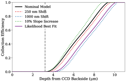
An extrapolation of the P concentration from the SIMS result with an exponential function suggests that the transition from the ISDP layer to the bulk value of cm-3 occurs over a distance of m. The P concentration determines the transport properties (mobility, lifetime) of the free charge carriers and the electric field profile, which control the fraction of the free charge carriers that survive recombination. We perform a numerical simulation to estimate the charge collection efficiency as a function of depth from the P concentration profile, with details provided in Appendix A. The nominal result, which shows a transition from zero to full charge collection over m (from 4 to 9 m from the backside surface), is presented by the black line in Fig. 8.
The exact location and profile of the PCC region has a significant impact on the spectral shape of radioactive decays originating on the backside of the CCDs, specifically 210Pb and 210Bi decays just below the ISDP layer, which were originally on the backside of the wafer (see Section III.3). To quantify the systematic uncertainty that PCC introduces in our background model, we compare simulated events on the back of the CCDs under different PCC-model assumptions. We vary the slope and position of the PCC curve and analyze the resulting spectra from backside 210Pb and 210Bi decays. Three examples from this ensemble are shown by the dotted lines in Fig. 8. The spectral difference between the nominal and varied models can be generally parametrized by the function:
| (7) |
where the amplitude depends on the specific PCC model and is primarily sensitive to the distance between the backside and the depth at which the collection efficiency “turns on.” We find a single to describe well all models in the ensemble, reducing Eq. (7) to depend on a single parameter .
As shown in the inset of Fig. 8, the parametrization describes the spectral differences well at low energies where they are most significant. The accuracy of the parametrization worsens above keVee, which only accounts for of the spectral difference and is negligible compared to the statistical uncertainty of the measured spectrum for the WIMP search.
The SIMS profile also shows an unexpectedly high concentration of hydrogen in the 1 m thick ISDP region. While the origin of the hydrogen is unknown, it likely is captured during the deposition of the ISDP layer, which occurs at C in the presence of SiH4 and PH3 gases Pejnefors et al. (1999). The hydrogen itself is not a problem but likely contains trace levels of radioactive tritium. Given the hydrogen concentration of H/cm3 measured by SIMS and the approximation that the tritium content in hydrogen in both of these gases is comparable to water ( 3H/H Plastino et al. (2007, 2011)), we expect tritium activities in the ISDP layer on the order of 1–30 mBq kg-1. This is higher than the final best-fit activity of bulk 3H that we find from direct silicon activation, but due to the low mass of the ISDP layer, it only amounts to 10–300 nBq per CCD (less than one decay per month). Moreover, our simulations suggest that only a small fraction of the low energy ’s originating in the ISDP layer penetrate into the charge collection region and contribute to the observed event rate. Thus, we exclude this background from our model.
IV Background Model
For comparison with data, our understanding of radioactive background sources and detector response must be converted into a background model: the expected distribution of ionization events in our CCDs in energy and depth. We construct the background model from a fit to data from CCDs 2–7 above 6 keVee with templates generated from our GEANT4 simulation output. We validate the fit result with CCD 1 above 6 keVee and demonstrate consistency with independent estimates of 210Pb surface activity from individual event identification. The background model is extrapolated below 6 keVee for our WIMP search.
IV.1 Template Fitting
We perform a binned-likelihood Poisson template fit to data in space starting from the over combinations of GEANT4 simulations for each isotope-volume. We consider events reconstructed by our fast clustering algorithm with energies between 6–20 keVee, where we do not expect a WIMP signal since other silicon-based experiments have placed strong bounds on WIMP masses that populate this high-energy range ( GeV) Agnese et al. (2013b). Although reconstructed events begin to saturate pixels above 14 keVee, we consider clusters up to 20 keVee that do not have a saturated pixel to accept the full tritium spectrum, which is expected to be a dominant bulk component. We develop the background-model construction on a subset (64) of the data, adding the remaining data for the final background model once the methodology has been fixed. We reserve all data from CCD 1 as a further cross-check, since the background environment in this CCD is different from CCDs 2–7.
We group like-simulations together according to common materials and decay chains. The grouping for materials is according to the detector parts in Table 1, with further subdivision of the copper into the OFHC copper vessel, box, and modules (because of their different activation histories), and the EFCu CCD 1 module. All EFCu is assumed to be perfectly radiopure, as it contributes count kg-1 day-1 keVee-1. For each detector part, we further group simulated isotopes by decay chain, according to Table 2. To avoid introducing uncertainty from the limited statistics of subdominant components, we discard any simulations that result in fewer than 0.1 events kg-1 day-1 and less than 1000 simulated events reaching the CCDs, leaving 289 simulations. The result of this grouping is 49 distinct sets of simulations, from which we construct templates (one per set).
For template , the number of expected events in bin (of width 0.25 keVee in and 0.025 pixels in ) is calculated by summing over the integer number of events in each binned simulation output normalized by the corresponding template activity in Table 1, the mass of the material simulated , the efficiency-corrected exposure of the data (), and the efficiency-corrected number of decays simulated according to
| (8) |
The efficiencies of the data and simulation are different since we find that the cluster selection on simulation to be 97.0, higher than the 93.3 observed for the data (Fig. 4). Additional study determines that the selection efficiency for simulated events varies slightly with depth, being nearly fully efficient at the front of the CCD and closer to 96 efficient at the back; this percent-level effect is noted but not taken into account in this analysis. No energy dependence in these efficiencies was observed. Furthermore, we include in a correction for the fraction of the CCDs that are masked (6.5%) rather than applying the iron mask (see Section II.3) to maximize the simulation statistics.
In total, the data is divided into 2464 bins, 56 in energy between 6–20 keVee and 44 bins in between 0.1–1.2 pixels. We implement a custom binned likelihood fit using TMinuit to compare the observed number of events in each bin against the expected number of events from simulation , obtained from the addition of the simulated templates with scaled amplitudes:
| (9) |
Under the assumption that the probability of observing events in a bin from an expectation of is determined by a Poisson distribution, the two-dimensional log-likelihood is then calculated to be the sum over all energy and bins as
| (10) |
We introduce Gaussian constraints as additional terms in the total log-likelihood for the subset of templates for which there is an independent estimate of the corresponding radioactivity:
| (11) |
where is the expected value of the scale factor of the template with uncertainty based on the measurement of the activity. For species for which the constraint comes from a measurement, the uncertainty is taken from Table 1. For upper limits, the Gaussian constraint is only included when exceeds the upper limit with an uncertainty of 10%. For the activation of the copper, which is not measured but calculated according to Eq. (5), we assume a 10 uncertainty. The tritium activity in the silicon bulk and all surface 210Pb templates are unconstrained in the fit.
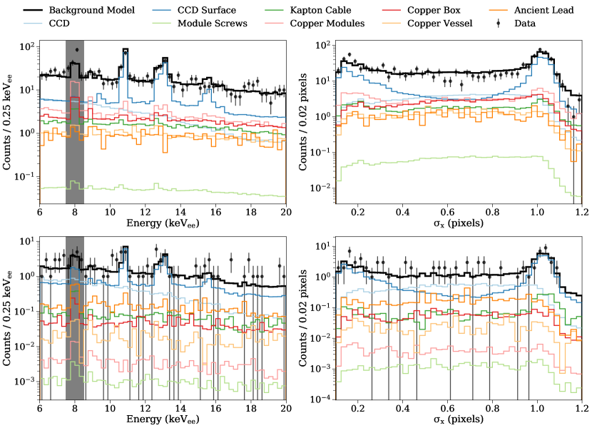
We minimize for the combined 2D spectra for CCDs 2–7. We exclude from the fit the 7.5–8.5 keVee region (removing 176 bins) because we are not confident in our prediction of the amplitude of the copper fluorescence peak with GEANT4. The result of the fit for CCDs 2–7, projected onto the fast-clustered energy and axes, is shown in Fig. 9, along with the cross-check using CCD 1. We also compared the background model prediction of the distribution of clusters to the data and find both to be statistically consistent with a uniform distribution. We provide a full list of best-fit scaling factors for each template in Table 3, along with calculated differential rates in different energy ranges. Note that the “fast clustering” algorithm used in the construction of the background model does not efficiently reconstruct events below 1 keVee (see Fig. 4), so the background model construction is effectively blind to the energy range most relevant for the WIMP search.
For the fit to CCDs 2–7, we find a goodness of fit -value of 0.004, as determined from the distribution of Monte Carlo trials drawn from the best fit PDF. In Appendix B, we detail this procedure and show how this poor goodness of fit is dominated by outlier bins above 14 keVee, where saturation is likely not being perfectly modeled. Moreover, we show that removing outlier bins in the saturation region and performing the same procedure results in an improved -value of 0.049 and less than change in the background model for any region of and depth below 6 keVee. Thus, we conclude that the background model constructed from data between 6–20 keVee, is statistically consistent with that same data below 14 keVee.
| Detector Part | Chain | Best-Fit Activity | Rate (dru): CCDs 2–7 | Rate (dru): CCD 1 | ||||
| 1–6 keVee | 6–20 keVee | 1–6 keVee | 6–20 keVee | |||||
| 1 | CCD | 238U | 0.897 | Bq/kg | 0.01 | 0.01 | ||
| 2 | CCD | 226Ra | 0.900 | Bq/kg | 0.01 | 0.01 | ||
| 3 | CCD | 232Th | 0.900 | Bq/kg | 0.01 | 0.03 | 0.01 | 0.02 |
| 4 | CCD | 40K | 0.910 | Bq/kg | ||||
| 5 | CCD | 22Na | 1.066 | Bq/kg | 0.17 | 0.16 | 0.10 | 0.09 |
| 6 | CCD | 32Si | 1.042 | Bq/kg | 0.19 | 0.17 | 0.15 | 0.13 |
| 7 | CCD | 3H | 1.131 | Bq/kg | 2.86 | 0.78 | 2.40 | 0.66 |
| 8 | CCD (front surf.) | 210Pb | 1.658 | nBq/cm2 | 1.45 | 1.67 | 0.53 | 0.88 |
| 9 | CCD (back surf.) | 210Pb | nBq/cm2 | |||||
| 10 | CCD (wafer surf.) | 210Pb | 1.343 | nBq/cm2 | 2.43 | 1.84 | 1.98 | 1.18 |
| 11 | Copper Box | 238U | 0.900 | Bq/kg | 0.01 | 0.01 | ||
| 12 | Copper Box | 226Ra | 0.900 | Bq/kg | 0.19 | 0.15 | 0.03 | 0.02 |
| 13 | Copper Box | 210Pb | 0.380 | mBq/kg | 0.33 | 0.20 | 0.02 | 0.01 |
| 14 | Copper Box | 232Th | 0.900 | Bq/kg | 0.08 | 0.06 | 0.01 | 0.01 |
| 15 | Copper Box | 40K | 0.900 | Bq/kg | ||||
| 16 | Copper Box | Act. | 1.015 | Bq/kg | 0.63 | 0.49 | 0.10 | 0.08 |
| 17 | Copper Modules | 238U | 0.900 | Bq/kg | 0.05 | 0.03 | ||
| 18 | Copper Modules | 226Ra | 0.900 | Bq/kg | 0.21 | 0.17 | ||
| 19 | Copper Modules | 210Pb | 0.557 | mBq/kg | 1.18 | 0.71 | ||
| 20 | Copper Modules | 232Th | 0.900 | Bq/kg | 0.10 | 0.08 | ||
| 21 | Copper Modules | 40K | 0.900 | Bq/kg | ||||
| 22 | Copper Modules | Act. | 1.006 | Bq/kg | 0.30 | 0.23 | 0.01 | 0.01 |
| 23 | Kapton Cable | 238U | 1.016 | mBq/kg | 0.51 | 0.30 | 0.23 | 0.11 |
| 24 | Kapton Cable | 226Ra | 1.362 | mBq/kg | 0.24 | 0.18 | 0.05 | 0.03 |
| 25 | Kapton Cable | 232Th | 1.010 | mBq/kg | 0.17 | 0.13 | 0.04 | 0.02 |
| 26 | Kapton Cable | 40K | 1.003 | mBq/kg | 0.09 | 0.05 | 0.04 | 0.02 |
| 27 | Kapton Cable | Act. | 1.000 | Bq/kg | 0.01 | 0.01 | ||
| 28 | Ancient Lead | 238U | 0.911 | Bq/kg | ||||
| 29 | Ancient Lead | 226Ra | 0.900 | Bq/kg | 0.44 | 0.36 | 0.21 | 0.18 |
| 30 | Ancient Lead | 210Pb | 1.000 | mBq/kg | 0.04 | 0.03 | 0.24 | 0.18 |
| 31 | Ancient Lead | 232Th | 1.000 | Bq/kg | ||||
| 32 | Ancient Lead | 40K | 0.916 | Bq/kg | ||||
| 33 | Outer Lead | 238U | 0.916 | Bq/kg | ||||
| 34 | Outer Lead | 226Ra | 0.909 | Bq/kg | ||||
| 35 | Outer Lead | 210Pb | 1.000 | Bq/kg | ||||
| 36 | Outer Lead | 232Th | 0.907 | Bq/kg | ||||
| 37 | Outer Lead | 40K | 0.906 | Bq/kg | ||||
| 38 | Module Screws | 238U | 1.000 | mBq/kg | ||||
| 39 | Module Screws | 226Ra | 0.900 | mBq/kg | 0.01 | 0.01 | ||
| 40 | Module Screws | 210Pb | 1.000 | mBq/kg | ||||
| 41 | Module Screws | 232Th | 1.024 | mBq/kg | 0.02 | 0.01 | ||
| 42 | Module Screws | 40K | 1.000 | mBq/kg | ||||
| 43 | Module Screws | Act. | 1.000 | Bq/kg | ||||
| 44 | Copper Vessel | 238U | 0.903 | Bq/kg | ||||
| 45 | Copper Vessel | 226Ra | 0.900 | Bq/kg | 0.10 | 0.09 | 0.01 | 0.01 |
| 46 | Copper Vessel | 210Pb | 0.731 | mBq/kg | 0.06 | 0.03 | ||
| 47 | Copper Vessel | 232Th | 0.900 | Bq/kg | 0.04 | 0.03 | ||
| 48 | Copper Vessel | 40K | 0.901 | Bq/kg | ||||
| 49 | Copper Vessel | Act. | 0.486 | Bq/kg | 0.33 | 0.27 | 0.05 | 0.04 |
| Total | 12.28 | 8.29 | 6.22 | 3.70 | ||||
IV.2 Surface 210Pb Analysis
One of the unique features of the CCD technology as a particle detector is the ability to identify events coming from the same decay chain over long time periods. Recently, the DAMIC Collaboration published an analysis of spatially coincident and events with time separation up to weeks to measure 32Si bulk contamination and set upper limits on bulk 210Pb, 238U, and 232Th Aguilar-Arevalo et al. (2021). The 210Pb limits were set under the assumption that all measured coincident 210Pb-Bi decays occurred in the bulk silicon. In reality, these events are far more likely to originate from 210Pb deposited on the external surfaces of the CCD and silicon wafer by radon plate-out, as in our background model. Here, we compare the results from the background model fit with the number of 210Pb-Bi event pairs from Ref. Aguilar-Arevalo et al. (2021), under the assumption that these events originate from the surfaces of the CCDs.
We briefly summarize the analysis from Ref. Aguilar-Arevalo et al. (2021). We used 181.3 days of data in 1x1 format instead of the data in 1x100 format used for most of the analysis presented in this paper. The detector setup was the same but the data was acquired earlier, with data acquisition starting before CCD 2 became operational so it was not included in the analysis. Classification of ’s and ’s was based on the variable , the fraction of pixels over threshold in the smallest rectangle containing the clustered pixels. This selection was tuned on simulation to correctly classify of all simulated ’s and 100% of ’s with energies MeV. For two events to qualify as a coincident 210Pb-Bi candidate, they must both be classified as ’s, occur within the same CCD in images less than 25 days apart ( of 210Bi), include a minimum of one pixel overlap, and the energy of the first must be reconstructed in the range 0.5–70 keVee. In total, 69 event pairs were found in the six CCDs with an exposure of 6.5 kg-days.
As presented in Table 3, we find a best-fit 210Pb activity of () nBq/cm2 for the front (wafer back) surface in our background model fit. To translate the fit result to the expected number of 210Pb-Bi event pairs observed in Ref. Aguilar-Arevalo et al. (2021), we first determine the selection efficiencies for front (wafer back) surface 210Pb-Bi decay sequences from 50,000 GEANT4 simulated decays to be . The wafer back surface has a higher selection efficiency because it is closer to the active bulk, meaning that, despite the PCC region, it has a higher probability for both decays in a sequence to be reconstructed and tagged. As in Ref. Aguilar-Arevalo et al. (2021), the time efficiency to select decay sequences is because of the readout time between images and the detector downtime. Given the surface area of 38 cm2 of each CCD, () event pairs are expected from front (wafer back) surface 210Pb. Additionally, accidental event pairs are expected from random events overlapping spatially, and event pairs are expected from 32Si-P decays. The resulting expected 210Pb-Bi pairs is slightly larger than the 69 candidate pairs observed.
We also compare the background model fit result to the observed number of ’s in the front and the back of the CCDs. As shown in Ref. Aguilar-Arevalo et al. (2021), front and back ’s can be distinguished by the aspect ratio of the clusters through a selection on . Furthermore, the energy of most of the observed ’s is consistent with the decay of surface 210Po, daughter of 210Bi, with an energy distribution peaked at 5.3 MeV and a long tail toward lower energies caused by energy losses in the CCD dead layers. Assuming secular equilibrium along the 210Pb-Bi-Po chain, the fit result corresponds to () 210Po decays in the front (wafer back) of each CCD in the data set used in Ref. Aguilar-Arevalo et al. (2021). The total observed number of ’s cannot be directly compared to these values since they include the contribution from 210Po decays on the copper surrounding the CCDs444The observation of 210Po ’s from the copper does not imply a presence of 210Pb on the copper surface since the copper cleaning procedure is known to be more efficient in removing 210Pb than 210Po Bunker et al. (2020).. However, assuming that the contribution from the copper is the same to the front and back CCD surfaces (treating CCD 1 separately, and excluding the top and bottom surfaces of the stack of CCDs 2–7), the front-back difference in the number of 210Po decays per CCD, , can be compared. We estimate the number of surface 210Po decays from the number of ’s with energy MeV. This selection excludes higher energy ’s from other decays in the U and Th chains, while retaining 95% of surface 210Po decays that deposit energy in the CCDs. After applying a simple geometrical simulation to estimate the event acceptance, we obtain from counting, compared to from the background model fit.
Overall, we regard the variation (considering only statistical uncertainties) between the background model fit result and the 210Pb-Bi and 210Po counting exercises as satisfactory. These cross checks generally confirm the magnitude of 210Pb contamination on the CCD surfaces, and the relative contamination between the front and the back of the CCDs. We remind the reader that the 210Pb surface activity was left unconstrained in the template fit (Sec. IV.1).
IV.3 Extrapolation
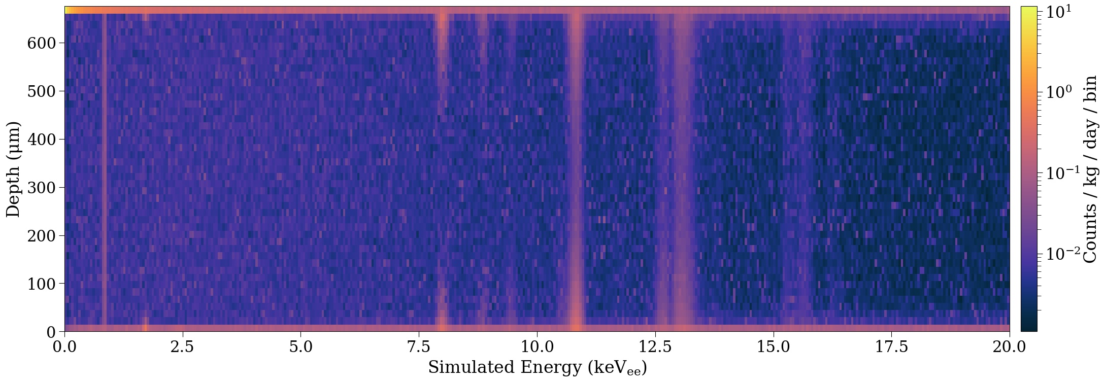
Following this fit, we use the simulation output to construct a single template for our background model in simulated variables vs. according to the best-fit scale factors . Before adding the contributions from each individual template , we remove any remaining statistical anomalies. For any template that contributes a total integral of less than 0.1 events/kg-day between 0–20 keVee (less than 1 event in the WIMP search), we average over by overwriting the content of all bins for the same with their mean value. This smooths templates (2), 4, 9, (11), 15, (17–20), 21, (27), 28, 31–38, (39), 40, (41), 42–44, (47), and 48, where templates in parentheses are smoothed only for CCD 1. Refer to Table 3 for template identification. Second, after adding the templates, we scan for any anomalously high bins, defined as being 20 standard deviations away from the mean of the bulk background and not adjacent to another high bin (as in an energy peak). In total, 3 (4) bins are removed for CCDs 2–7 (CCD 1), which account for a total rate of 0.07 (0.16) events/kg-day, or less than 1 event in the combined exposure. The resulting background model template for CCDs 2–7 in simulated coordinates is shown in Fig. 10. In order to maximize our resolution at this stage, we choose fine binning of 10 eVee in and 15 m in . The background model has a bulk background rate of () counts kg-1 day-1 keVee-1 between 2.5–7.5 keVee in CCD 1 (CCDs 2–7), where the error bars provided are statistical, and an implicit energy threshold set by GEANT4 of eVee555The Livermore physics list is validated down to 250 eV Cirrone et al. (2010); Pandola et al. (2015), and we independently extend this validation down to 50 eVee using our data Da Rocha (2019)..
In Section IV.1, we constructed the background model using a fit to only data from CCDs 2–7, excluding data from CCD 1. CCD 1 is treated separately since the overall background rates are roughly lower than in CCDs 2–7, primarily because of the EFCu module and additional ancient lead shield. Using simulated events for CCD 1 and the best-fit parameters , we construct an analogous background model for CCD 1. Any event will be compared against the relevant background model according to the CCD in which it was measured.
While the background model represents our best fit above 6 keVee, there is still substantial uncertainty in our PCC model at lower energies (Section III.6). This uncertainty is restricted to the highest -bin (back of the CCD) in Fig. 10, and can be approximated as an additive correction proportional to keV-1/2). Furthermore, there is an underlying, approximately constant spectrum in the highest -bin from ionization events in the fully-depleted region of the CCDs, thus we split the background model shown in Fig. 10 into two pieces: a “lower-bound” background model with the exponential PCC correction subtracted, such that the background rate in the highest bin is approximately flat in energy, and a positive, additive component proportional to keV-1/2). We treat the positively valued amplitude of the additive exponential as a free parameter in our WIMP-search fit. We perform this procedure for the CCD 1 and CCDs 2–7 background models separately and find that the exponential component in CCD 1 corresponds to the same fraction of events in the highest bin as in CCDs 2–7, but its amplitude is 25% smaller due to the lower background rates in CCD 1 external to the sensor. Thus, to reduce the number of free parameters in our WIMP-search fit, we fix the ratio of the additive exponential component between CCDs 2–7 and CCD 1 to 75%.
We perform the WIMP-search fit on events identified by the “likelihood clustering” algorithm presented in Section II.3, which is designed to efficiently identify low-energy clusters on full CCD images. Thus, we need to translate the final background model in simulated coordinates into reconstructed coordinates by the likelihood clustering algorithm, correctly accounting for all reconstruction efficiencies in the data down to our analysis threshold of 50 eVee.
| Parameter | Null hypothesis | All events | CCD 1 only | CCDs 2–7 only | 200 eVee | |
|---|---|---|---|---|---|---|
| [events] | 0 | 0 | ||||
| [eVee] | - | - | ||||
| [events] | 56.2 | - | ||||
| [events] | 625 | - | ||||
| [events] | 5.4 | - | ||||
| [events] | 41.6 | - | ||||
| exposure [kg-day] | - | 10.9 | 1.6 | 9.3 | 10.9 | 10.3 |
| no-signal -value | - | 0.039 | 1 | |||
| g.o.f. -value | - | 0.10 | 0.94 | 0.21 | 0.32 | 0.69 |
We sample from the background model (both the lower bound and the additive exponential component) separately for CCDs 2–7 and CCD 1 to obtain and values for simulated events. We then apply the CCD-response simulation (diffusion, binning, saturation, etc.) and add the pixel values from the events randomly onto blank images. To best represent the data, we also add shot noise from leakage current to the simulated images at the levels measured for the exposed images. A total of 830 simulated images with 250 randomly sampled events each (for a total of 200,000 simulated events per CCD) is then run through the same analysis pipeline as the data (including masking, likelihood clustering and cluster selection) to obtain the final simulated clusters and their reconstructed coordinates. Unlike the analysis that is performed to translate simulated GEANT4 events into reconstructed clusters in Section IV.1, this procedure accurately reflects data all the way down to our analysis threshold of 50 eVee, and implicitly accounts for all reconstruction efficiencies, solely at the cost of processing time. The only efficiency correction that must be made is for the removal of clusters that overlap or contain more than one ionization event (see Section II.3), which is higher in the simulated images because of the higher spatial density of events.
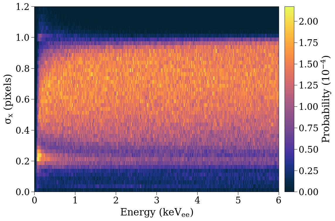
We generate the response PDF of our detector (Fig. 11) by repeating the procedure above with events sampled uniformly in energy and depth. For a model of the hypothetical WIMP signal, we scale the response PDF as a function of energy according to the signal spectrum.
V Low Energy Analysis
We perform a WIMP search by comparing the data below 6 keVee to the background model constructed in Section IV.3. The results, reported in Ref. Aguilar-Arevalo et al. (2020), are summarized and expanded below.
Images correlated with periods of higher leakage current due to LED flashing and temperature cycling show a large increase in the total number of clusters and were excluded from the WIMP search. These 443 images (8% of the total) were identified as those that have an average charge per pixel larger than (6.76 ADU average pixel value). Their removal results in a total exposure for the WIMP search of 10.93 kg-days. These images were used in the background model construction, since the higher leakage current has no effect above 6 keVee.
A two-dimensional unbinned likelihood fit was performed to the final sample of events identified by the likelihood clustering following the formalism in Ref. Aguilar-Arevalo et al. (2016). The fit was performed jointly to the two data sets from CCD 1 and CCDs 2–7, each containing events in a fractional exposure . The fit function was constructed from the addition of probability density functions (PDFs) of the lower-bound background model , the PCC correction , and a “generic signal” of a population of events distributed uniformly in space with an exponentially decreasing spectrum :
| (12) |
where the exponential decay is multiplied with our detector response function shown in Fig. 11. We choose this functional form to capture the most general DM models, such as the quenched Chavarria et al. (2016) WIMP nuclear recoil spectrum. The decay energy and amplitude of a generic signal, the amplitudes of the lower-bound background models , and the PCC correction666We note that is a single free parameter because , as described in Section IV.3. were free parameters in the fit. We constrained to , the predicted normalization from the background model fit above , with fractional uncertainty . We perform the fit in the region (excluding Si fluorescence ) and pixel by minimizing with MINUIT the extended negative log-likelihood function:
| (13) |
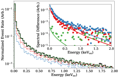
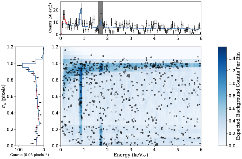
Figure 12 shows the comparison between the best-fit background model (in blue) and data (markers). The best-fit values for the lower-bound number of background events are and . The best-fit value for and corresponds to a distance between 210Pb contamination on the back side of the original wafer and the start of charge collection of m (see purple line in Fig. 8). Our best fit exhibits a preference for an exponential bulk component with events and eVee. We estimate a goodness-of-fit -value of 0.10 from the minimum negative log-likelihood distribution obtained from running the fit procedure on Monte Carlo samples drawn from the best-fit PDF. Note that the outlier first bin in the projection arises from front-side events above 1 keVee.
We computed the uncertainty about the best fit by performing likelihood ratio tests between the global best fit and fit results with constrained values of and . Figure 13 shows the probability of the parameter space derived from the likelihood-ratio test statistic assuming that its distribution follows a distribution with two degrees of freedom (Wilks’ theorem). We confirmed by Monte Carlo that Wilks’ theorem is an appropriate approximation for our data. The background-only hypothesis is disfavored with a -value of (). Figure 14 shows the bulk excess spectrum obtained by projecting the best-fit result onto the energy axis and subtracting the best-fit background model amplitude, which includes the partial charge collection component. The band was derived from the contour in Fig. 13. The displayed error bars are the Poisson uncertainties in the bin contents since the uncertainty in the background model amplitude is small in comparison. The energy bins below 200 eVee show a clear excess above background with a spectrum that is well described by the best-fit generic signal model. Furthermore, we confirm that events with energies below 200 eVee are distributed uniformly in and time, as expected for a dark matter signal.
Several systematic tests were performed to confirm the consistency of our fit result, with results summarized in Table 4:
-
•
If we perform the fit to events with energies 200 eVee only, the result is consistent with the background-only hypothesis and shows no preference for a generic signal.
-
•
If we perform the fit to the data from CCD 1 or CCDs 2–7 separately, the resulting generic signal is statistically consistent between the two datasets with a higher statistical significance in CCD 1, which has the lowest background.
-
•
A comparison between the two-dimensional profile of the best-fit generic signal and the additive PCC component (Fig. 15) shows that the excess of events with pixel that drive the statistical significance of the generic signal are in a region of parameter space that is not populated by events from the CCD backside.
-
•
Although front-surface () events can populate the region of parameter space with pixel, a fit to the data after removing clusters where only one pixel has a value greater than 1.6 —a selection that removes 56% of front-surface events but only 6.5% of bulk events—still returns a statistically significant generic signal with values for and consistent with the original result Aguilar-Arevalo et al. (2020).
-
•
If we introduce in our fit an artificial energy offset in the generic signal spectrum Dessert et al. (2021), we only observe a statistically significant excess for offsets below 100 eVee, which further confirms that our background model describes the data well above 200 eVee, and that the reported signal excess does not originate from unexpectedly large statistical fluctuations in the data.
Events occurring in the proximity of the serial register Moroni et al. (2021a) were excluded as a possible source for the observed excess. These events generate ionization charge in the field-free regions peripheral to the CCD active region that can diffuse and reach the serial register. Clusters from these events appear as horizontal streaks in 1x1 images. In 1x100 images, where clusters appear as horizontal sequences of contiguous pixels, it is not possible to identify serial register events from their topology. However, since any charge in the serial register is discarded before the image is read out, serial register events that occur during an exposure are excluded from the analysis. Serial register events are only a problem if they occur during CCD readout. However, CCD readout accounts for only 0.01 of the overall target exposure and contributes a negligible number of clusters, as verified with blank images.
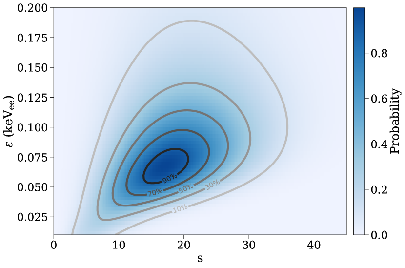
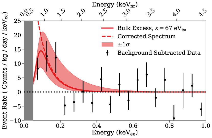
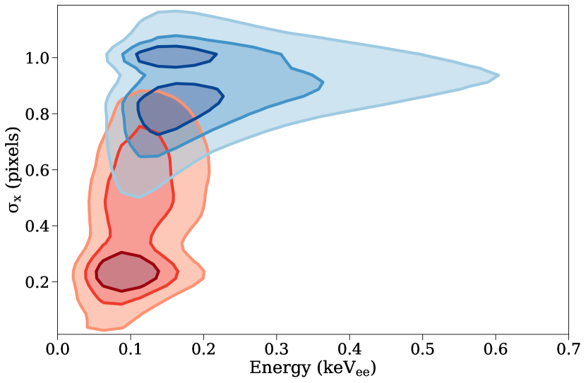
Our analysis suggests the presence of bulk ionization events at a rate of a few per kg-day in the range with a uniform distribution in the bulk silicon whose source is not included in our background model. The origin of these events (e.g., whether they are electronic or nuclear recoils, or some unexpected instrumental effect) remains unknown. In Ref. Aguilar-Arevalo et al. (2020), we employ the background model presented here to set the most stringent limits with a silicon target on the WIMP-nucleon spin-independent scattering cross section for WIMP masses in the range .
VI Conclusion
In this paper, we present the first comprehensive background model for a CCD detector down to an unprecedentedly low energy of 50 eVee. The background model shows excellent agreement with the data down to 200 eVee, with an unexpected and statistically significant excess of events at the lowest energies discussed in Section V.
In the process of constructing this background model, we compiled and determined the relative contributions of various radioactive background sources. We note that our dominant background (see Table 3) comes from cosmogenic 3H in the bulk of our CCDs and 210Pb deposited on the surfaces of the CCDs, including the surface of the wafer prior to CCD fabrication, now embedded m beneath the CCD back surface.
The measured activity of bulk 3H from the template fit allows us to determine (according to the exposure history of our CCDs) the activation rate of cosmogenic 3H in silicon. Under the assumption that activation of the pure silicon starts at with the formation of the original ingot used to produce the wafers (total sea-level equivalent exposure time years), we obtain a sea-level equivalent activation rate of atoms/kg-day. Alternatively, if we assume that coincides with CCD fabrication (total sea-level equivalent exposure time years), during which the wafers were briefly processed at C, potentially “baking-out” any 3H in the silicon, we obtain an activation rate of atoms/kg-day777The larger uncertainty in this case comes from not knowing at what dates in the fabrication process the baking took place and which flights come after this step.. Both of these numbers are consistent with recent measurements Saldanha et al. (2020), which leaves the possibility that the activation clock for tritium may be “reset” during CCD fabrication. Under the assumption that 22Na cannot be baked out from the wafers888In fact, Na does have significant mobility in silicon at high temperatures Korol (1988); Zastavnoi and Korol’ (2016), but this warrants further study., we constrain the sea-level activation rate of 22Na in silicon to be atoms/kg-day, in excellent agreement with Ref. Saldanha et al. (2020).
The fit chooses to place 210Pb surface contamination on the front of the CCD and the back of what was originally the silicon wafer, the two surfaces most likely to contain such contamination (despite no input bias towards these surfaces in the fit). Furthermore, the fit returns slightly more contamination on the front of the CCD than on the back of the wafer. The measured activities and locations of 210Pb surface contamination from the template fit were confirmed by an independent analysis that leverages on the high spatial resolution of CCDs (Section IV.2), used previously to constrain radiocontaminants in the bulk silicon Aguilar-Arevalo et al. (2021). These results demonstrate that our fitting methodology can effectively discern between different spectral components that originate from different locations in the detector.
In our modeling of the response of the detector to surface backgrounds, we discovered that diffusion of phosphorous from the backside ISDP layer into the high-resistivity bulk silicon causes a region of significant charge recombination that extends a few m into the CCDs (Section III.6). Partial charge collection (PCC) in this region causes a significant distortion of the spectrum from 210Pb decays on the backside of the CCDs, which is the dominant systematic uncertainty in our WIMP-search fit. Our PCC profile, obtained from the measured properties of minority-carrier transport in silicon (details in Appendix A), was experimentally confirmed with direct measurements using a 55Fe x-ray source in Ref. Moroni et al. (2021b). High levels of hydrogen were also measured in the ISDP layer. This hydrogen is expected to contain minute levels of tritium, which due to the proximity to the PCC region, are expected to be preferentially reconstructed at the low energies where a WIMP signal is expected. Although the background rate from 3H decays in the ISDP region is too small to be observable with this analysis, it could become a problem for future CCD dark matter experiments with greater sensitivity.
This analysis lays the foundation for the background modeling for the upcoming DAMIC-M experiment Settimo (2020) and will inform the analysis and design of other CCD dark matter experiments (e.g., SENSEI Crisler et al. (2018) and Oscura Kolb et al. (2018)). It demonstrates the importance of limiting cosmogenic activation of the silicon and exposure of the detector surfaces to radon, including on the wafers prior to CCD fabrication. It identifies important low-energy backgrounds associated with the CCD backside that must be addressed for future CCD dark matter detectors, e.g., by removing m from the backside of the CCDs after fabrication Holland et al. (2003). Our background-model fit demonstrates the limitation of using ancient lead for shielding since the dominant external background in CCD 1 already comes from 210Pb decays in the ancient lead (Table 3), which motivates the development of new methods of radiation shielding for future large-scale solid-state dark matter detectors. Finally, successful mitigation of some of the identified backgrounds may require underground radon-free facilities for critical fabrication activities (e.g., sensor packaging, copper growth and machining, etc.) and further improvements in the design of dark matter detectors.
Acknowledgements.
We are grateful to SNOLAB and its staff for support through underground space, logistical and technical services. SNOLAB operations are supported by the Canada Foundation for Innovation and the Province of Ontario Ministry of Research and Innovation, with underground access provided by Vale at the Creighton mine site. We acknowledge financial support from the following agencies and organizations: National Science Foundation through Grants No. NSF PHY-1912766 and NSF PHY-1806974; Kavli Institute for Cosmological Physics at The University of Chicago through an endowment from the Kavli Foundation; Gordon and Betty Moore Foundation through Grant GBMF6210 to the University of Washington; Fermi National Accelerator Laboratory (Contract No. DE-AC02-07CH11359); Institut Lagrange de Paris Laboratoire d’Excellence (under Reference No. ANR-10-LABX-63) supported by French state funds managed by the Agence Nationale de la Recherche within the Investissements d’Avenir program under Reference No. ANR-11-IDEX-0004-02; Swiss National Science Foundation through Grant No. 200021_153654 and via the Swiss Canton of Zurich; Project PID2019-109829GB-I00 funded by MCIN/ AEI /10.13039/501100011033; Mexico’s Consejo Nacional de Ciencia y Tecnología (Grant No. 240666) and Dirección General de Asuntos del Personal Académico–Universidad Nacional Autónoma de México (Programa de Apoyo a Proyectos de Investigación e Innovación Tecnológica Grants No. IB100413 and No. IN112213); STFC Global Challenges Research Fund (Foundation Awards Grant ST/R002908/1).Appendix A Partial Charge Collection (PCC) Efficiency Model
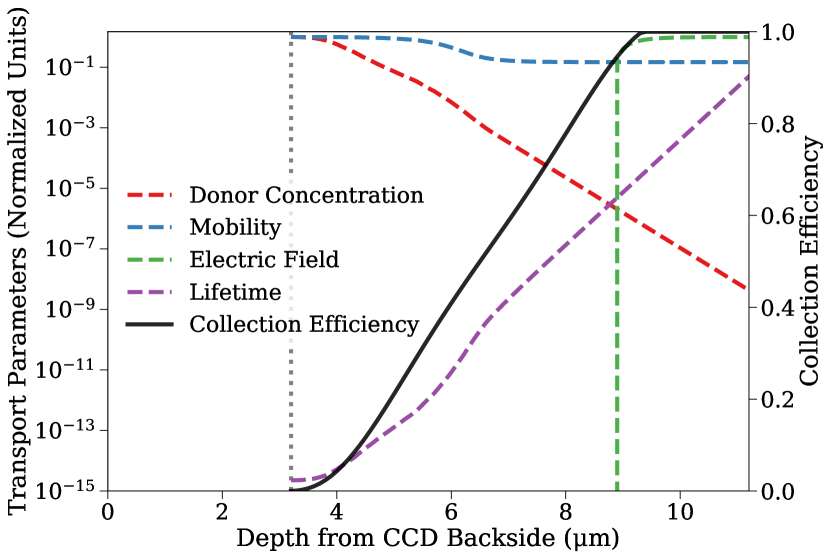
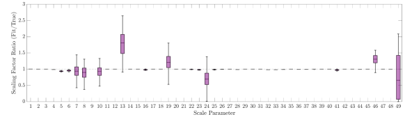
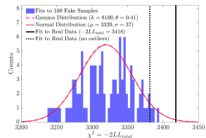
As discussed in Section III.6, the presence of the ISDP layer on the back of the CCD during fabrication leads to the diffusion of phosphorous into the bulk silicon. The SIMS measurements show that the donor concentration decreases from cm-3 at the backside contact to cm-3 in the CCD active region over a distance of . The concentration of donors changes the mobility and lifetime of the minority charge carriers (holes) del Alamo and Swanson (1987)Wang et al. (1990), and the electric field profile near the back of the CCD. These variations can be many orders of magnitude; Fig. 16 shows the P concentration and the resulting transport properties as a function of the distance from the CCD backside .
For , there is a field-free region where diffusion, a relatively slow process, is the only mechanism for charge to reach the fully-depleted active region, where it will be drifted and eventually collected at the CCD gates. At high P concentration close to the CCD backside, the carrier lifetime is very short and all charge recombines before diffusing significantly. However, at intermediate P concentration where is sufficiently long, some of the charge diffuses into the active region before it recombines, which creates the region of PCC. We calculated the collection efficiency as a function of by performing a numerical simulation of the evolution of charge packets. We assumed that and therefore the problem is invariant in the coordinates. We considered the region from the back surface of the original wafer to a point in the active region where any charge can be assumed to be efficiently drifted and collected at the CCD gates, i.e., . We divided the region into nm bins and assumed all charge in a given bin evolves in the same manner.
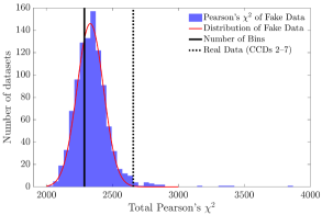
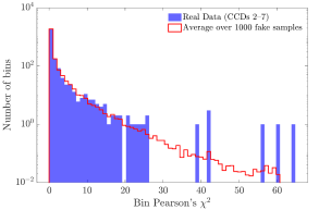
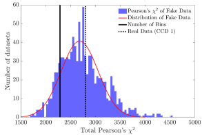
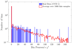
We placed a function of charge at a specific position and evolved the charge distribution in ps temporal steps. The spatial distribution evolves via two channels: diffusion and drift in the electric field. To simulate diffusion, the charge in each spatial bin is redistributed every time step following a Gaussian with variance Hopkinson (1987)
| (14) |
where is the Boltzmann constant, is the temperature, is the hole mobility, and is the fundamental charge. Additionally, the position of the charge drifts as
| (15) |
where and are the spatial bin positions of the charge before and after the time step, and is the component of the electric field. Finally, at each time step the charge carriers have some probability to recombine, thus the charge in each bin decreases as
| (16) |
which is a good approximation since in the PCC region.
After each time step, the charge that is collected by the CCD is defined as any charge that enters in the active region m. We ran the simulation for ns and repeated over a range of depths. For every initial , the charge left in the partial charge region at the end of the simulation was of the initial value. The charge collection efficiency is the ratio of the collected charge to the initial charge deposited.
Our numerical simulations suggests that below we collect no ionization charge. The collection efficiency turns on for and rises nearly linearly until full collection efficiency at .
Appendix B Systematic Checks on the Background Model
In this Appendix, we test whether the data used to construct the background model is statistically consistent with Monte Carlo samples drawn from that background model. In order to check for any biases in our two-dimensional binned likelihood fit to construct the background model, we draw 100 fake samples (of the same size as the data) from the best-fit background model PDF and re-run the fitting algorithm on them (Section IV.1). We compare the ratio of the template fit parameters between the 100 trials and the input “true” values (Table 3). Figure 17 uses a box-and-whisker plot to show the distribution of each fit parameter across all 100 trials relative to the input value. The only significant bias is to add extra 210Pb in the OFHC copper volumes (parameters 13, 19, and 46 in Table 3). This is not an issue for our WIMP analysis, and indicates that the best fit to data overestimates external 210Pb components. Notably, the dominant of these components (parameter 19—the copper modules) is the closest to its input value. The variation of the other dominant background components (parameters 7, 8, and 10) in the trial fits is within the interquartile range. The other noticeable variation (parameters 24 and 49) comes from poorly constrained templates which contribute to the overall background combined. While not visible given the y-scale, the largest remaining bias is to include less intrinsic 22Na and 32Si than in the background model (parameters 5 and 6), which is consistent with the fact that the background-model fit result (see Table 3) increases these templates by roughly the same fraction over the mean value of the Gaussian constraint. Thus, we conclude that the fit methodology is not significantly biased.
To estimate the goodness of the fit, we compare the minimum log-likelihood test statistic of the background-model fit to data to the distribution of the results from the fits to the 100 fake samples. We find that the data gives a worse fit than the fake samples (Fig. 18), which indicates some systematic inconsistency between the data and the best-fit background model. We obtain a -value of 0.0039 (2.7 discrepancy) from a one-sided -test based on a Gaussian fit to the distribution of the fake samples. A fit with a gamma function returns a scale parameter , significantly different than expected for a distribution. If we scale the values by a factor of 5 (), we can mimic a distribution with 16200 (2 times the gamma distribution shape parameter ) degrees of freedom. Thus, we can consider the goodness of fit to be (-value of 0.0041), similar to the result from the Gaussian fit. Both of these fits are shown in Fig. 18.
To understand the origin of this inconsistency, we draw an additional 1000 samples (of the same size as the data) from the best-fit background model PDF. For every sample, we compute the total Pearson’s and the corresponding contribution from each bin relative to the best-fit background model PDF. The left-hand side panels of Fig. 19 show the distribution of total Pearson’s for the fake data samples with results for CCDs 2–7 (CCD 1) in the top (bottom) panel. The corresponding result from the fit to the data is marked by the vertical dashed line. The right-hand side panels show the distribution of the contribution of bins to the Pearson’s averaged over all fake data samples compared to the distribution from the best-fit to data. Overall, we find excellent agreement between the generated samples and the data in CCD 1. For CCDs 2–7, three statistically outlier data bins result in a mismatch between data and the fake samples: 1 event with eVee and pixels, 3 events with eVee and pixels, and 2 events with eVee and pixels. Notably, all of these bins are at high energies where saturation occurs. Removing these outlier bins from the data does not substantially change the fit result ( effect below 6 keVee,) but does significantly improve the goodness-of-fit. Specifically, using the gamma distribution from before, the updated best fit to data results in (-value of 0.049). Therefore, we conclude that the discrepancy between the maximum likelihood of the fit samples compared to the data in Fig. 18 is not caused by any mismodeling that affects the extrapolation of our background model to the energy region for the WIMP search, and is primarily restricted to the saturation region above 14 keVee.
References
- Kolb and Turner (1990) E. W. Kolb and M. S. Turner, The Early Universe, Vol. 69 (CRC Press, 1990).
- Bertone and Hooper (2018) G. Bertone and D. Hooper, Rev. Mod. Phys. 90, 045002 (2018).
- Goodman and Witten (1985) M. W. Goodman and E. Witten, Phys. Rev. D 31, 3059 (1985).
- Lewin and Smith (1996) J. D. Lewin and P. F. Smith, Astroparticle Physics 6, 87 (1996).
- Schumann (2019) M. Schumann, J. Phys. G 46, 103003 (2019), arXiv:1903.03026 [astro-ph.CO] .
- Battaglieri et al. (2017) M. Battaglieri et al., in U.S. Cosmic Visions: New Ideas in Dark Matter (2017) arXiv:1707.04591 [hep-ph] .
- Zurek (2014) K. M. Zurek, Phys. Rep. 537, 91 (2014), arXiv:1308.0338 [hep-ph] .
- Hochberg et al. (2017) Y. Hochberg, T. Lin, and K. M. Zurek, Phys. Rev. D 95, 023013 (2017), arXiv:1608.01994 [hep-ph] .
- Essig et al. (2012) R. Essig, J. Mardon, and T. Volansky, Phys. Rev. D 85, 076007 (2012).
- Graham et al. (2015) P. W. Graham, I. G. Irastorza, S. K. Lamoreaux, A. Lindner, and K. A. van Bibber, Annual Review of Nuclear and Particle Science 65, 485–514 (2015).
- Davis (2017) J. H. Davis, Phys. Rev. Lett. 119, 211302 (2017), arXiv:1708.01484 [hep-ph] .
- Collar (2018) J. I. Collar, Phys. Rev. D 98, 023005 (2018).
- Lin (2019) T. Lin, PoS 333, 009 (2019), arXiv:1904.07915 [hep-ph] .
- Amaral et al. (2020) D. W. Amaral et al. (SuperCDMS Collaboration), Phys. Rev. D 102, 091101 (2020).
- Arnaud et al. (2020) Q. Arnaud et al. (EDELWEISS Collaboration), Phys. Rev. Lett. 125, 141301 (2020).
- Agnes et al. (2018) P. Agnes et al. (DarkSide Collaboration), Phys. Rev. Lett. 121, 111303 (2018).
- Aprile et al. (2019) E. Aprile et al. (XENON Collaboration), Phys. Rev. Lett. 123, 251801 (2019).
- Arnaud et al. (2018) Q. Arnaud et al. (NEWS-G Collaboration), Astroparticle Physics 97, 54 (2018).
- Aguilar-Arevalo et al. (2020) A. Aguilar-Arevalo et al. (DAMIC Collaboration), Phys. Rev. Lett. 125, 241803 (2020).
- Allison et al. (2016) J. Allison et al., Nucl. Instrum. Methods Phys. Res. A 835, 186 (2016).
- Aguilar-Arevalo et al. (2016) A. Aguilar-Arevalo et al. (DAMIC Collaboration), Phys. Rev. D94, 082006 (2016).
- Aguilar-Arevalo et al. (2019a) A. Aguilar-Arevalo et al. (DAMIC Collaboration), Phys. Rev. Lett. 123, 181802 (2019a).
- Chavarria (2020) A. E. Chavarria (DAMIC), J. Phys. Conf. Ser. 1342, 012057 (2020).
- Hoppe et al. (2014) E. Hoppe, C. Aalseth, O. Farmer, T. Hossbach, M. Liezers, H. Miley, N. Overman, and J. Reeves, Nucl. Instrum. Methods Phys. Res. A 764, 116 (2014).
- Hoppe et al. (2007) E. Hoppe, A. Seifert, C. Aalseth, P. Bachelor, A. Day, D. Edwards, T. Hossbach, K. Litke, J. McIntyre, H. Miley, S. Schulte, J. Smart, and G. Warren, Nucl. Instrum. Methods Phys. Res. A 579, 486 (2007), proceedings of the 11th Symposium on Radiation Measurements and Applications.
- Leonard et al. (2008) D. Leonard et al., Nucl. Instrum. Methods Phys. Res. A 591, 490 (2008).
- Abgrall et al. (2016) N. Abgrall et al., Nucl. Instrum. Methods Phys. Res. A 828, 22 (2016).
- Mclean et al. (2012) I. S. Mclean, B. L. Flaugher, T. M. Abbott, R. Angstadt, J. Annis, et al., Ground-based and Airborne Instrumentation for Astronomy IV 8446, 844611 (2012).
- Flaugher et al. (2015) B. Flaugher et al. (DES), Astron. J. 150, 150 (2015), arXiv:1504.02900 [astro-ph.IM] .
- Holland et al. (2003) S. Holland, D. Groom, N. Palaio, R. Stover, and M. Wei, IEEE Trans. Electron Devices 50, 225 (2003).
- Holland (1989) S. Holland, Nucl. Instrum. Methods Phys. Res. A 275, 537 (1989).
- Lecrosnier et al. (1980) D. Lecrosnier, J. Paugam, F. Richou, G. Pelous, and F. Beniere, Journal of Applied Physics 51, 1036 (1980), https://doi.org/10.1063/1.327732 .
- Alex et al. (1996) V. Alex, S. Finkbeiner, and J. Weber, Journal of Applied Physics 79, 6943 (1996).
- Janesick (2001) J. Janesick, Scientific Charge-coupled Devices, Press Monograph Series (Society of Photo Optical, 2001).
- Holland et al. (2003) S. E. Holland, D. E. Groom, N. P. Palaio, R. J. Stover, and Mingzhi Wei, IEEE Transactions on Electron Devices 50, 225 (2003).
- Krupka et al. (2006) J. Krupka, J. Breeze, A. Centeno, N. Alford, T. Claussen, and L. Jensen, IEEE Transactions on Microwave Theory and Techniques 54, 3995 (2006).
- Aguilar-Arevalo et al. (2021) A. Aguilar-Arevalo et al., Journal of Instrumentation 16, P06019 (2021).
- Aguilar-Arevalo et al. (2019b) A. Aguilar-Arevalo et al. (DAMIC Collaboration), Phys. Rev. Lett. 123, 181802 (2019b).
- Rodrigues et al. (2021) D. Rodrigues, K. Andersson, M. Cababie, A. Donadon, A. Botti, G. Cancelo, J. Estrada, G. Fernandez-Moroni, R. Piegaia, M. Senger, M. S. Haro, L. Stefanazzi, J. Tiffenberg, and S. Uemura, Nucl. Instrum. Methods Phys. Res. A 1010, 165511 (2021).
- Ramanathan et al. (2017) K. Ramanathan, A. Kavner, A. E. Chavarria, P. Privitera, D. Amidei, T.-L. Chou, A. Matalon, R. Thomas, J. Estrada, J. Tiffenberg, and J. Molina, Phys. Rev. D 96, 042002 (2017).
- Abe et al. (2018) K. Abe et al., Nucl. Instrum. Methods Phys. Res. A 884, 157 (2018).
- Orrell et al. (2016) J. Orrell, C. Aalseth, I. Arnquist, T. Eggemeyer, B. Glasgow, E. Hoppe, M. Keillor, S. Morley, A. Myers, C. Overman, S. Shaff, and K. Thommasson, Journal of Radioanalytical and Nuclear Chemistry 309 (2016), 10.1007/s10967-016-4732-6.
- Loach et al. (2016) J. Loach, J. Cooley, G. Cox, Z. Li, K. Nguyen, and A. Poon, Nucl. Instrum. Methods Phys. Res. A 839, 6 (2016).
- Lawson (2020) I. Lawson, Journal of Physics: Conference Series 1342, 012086 (2020).
- Arnquist et al. (2020) I. Arnquist, M. di Vacri, and E. Hoppe, Nucl. Instrum. Methods Phys. Res. A 965, 163761 (2020).
- Aguilar-Arevalo et al. (2015) A. Aguilar-Arevalo et al., Journal of Instrumentation 10, P08014 (2015).
- Cebrián (2017) S. Cebrián, Int. J. Mod. Phys. A 32, 1743006 (2017), arXiv:1708.07449 [nucl-ex] .
- Laubenstein and Heusser (2009) M. Laubenstein and G. Heusser, Applied Radiation and Isotopes 67, 750 (2009), 5th International Conference on Radionuclide Metrology - Low-Level Radioactivity Measurement Techniques ICRM-LLRMT’08.
- Baudis et al. (2015) L. Baudis, A. Kish, F. Piastra, and M. Schumann, Eur. Phys. J. C 75, 485 (2015), arXiv:1507.03792 [astro-ph.IM] .
- Huang et al. (2021) W. Huang, M. Wang, F. Kondev, G. Audi, and S. Naimi, Chinese Physics C 45, 030002 (2021).
- Wang et al. (2021) M. Wang, W. Huang, F. Kondev, G. Audi, and S. Naimi, Chinese Physics C 45, 030003 (2021).
- Saldanha et al. (2020) R. Saldanha, R. Thomas, R. H. M. Tsang, A. E. Chavarria, R. Bunker, J. L. Burnett, S. R. Elliott, A. Matalon, P. Mitra, A. Piers, P. Privitera, K. Ramanathan, and R. Smida, Phys. Rev. D 102, 102006 (2020).
- Agnese et al. (2019) R. Agnese et al. (SuperCDMS), Astropart. Phys. 104, 1 (2019), arXiv:1806.07043 [physics.ins-det] .
- Sato and Niita (2006) T. Sato and K. Niita, Radiation Research 166, 544 (2006).
- Bé et al. (2010) M.-M. Bé, V. Chisté, C. Dulieu, X. Mougeot, E. Browne, V. Chechev, N. Kuzmenko, F. Kondev, A. Luca, M. Galán, A. Nichols, A. Arinc, and X. Huang, Table of Radionuclides, Monographie BIPM-5, Vol. 5 (Bureau International des Poids et Mesures, Pavillon de Breteuil, F-92310 Sèvres, France, 2010).
- Pocar (2003) A. Pocar, Low Background Techniques and Experimental Challenges for Borexino and its Nylon Vessels, Ph.D. thesis, Princeton University (2003).
- Agnese et al. (2013a) R. Agnese et al. (SuperCDMSSoudan), Appl. Phys. Lett. 103, 164105 (2013a), arXiv:1305.2405 [physics.ins-det] .
- Ziegler et al. (1985) J. Ziegler, J. Biersack, and U. Littmark, The Stopping and Range of Ions in Solids, The Stopping and Range of Ions in Matter, Vol. 1 (Pergamon Press, 1985).
- Ziegler et al. (2010) J. F. Ziegler, M. D. Ziegler, and J. P. Biersack, Nucl. Instrum. Methods Phys. Res. B 268, 1818 (2010).
- Bunker et al. (2020) R. Bunker, T. Aramaki, I. Arnquist, R. Calkins, J. Cooley, E. Hoppe, J. Orrell, and K. Thommasson, Nucl. Instrum. Methods Phys. Res. A 967, 163870 (2020).
- di Vacri et al. (2021) M. di Vacri, I. Arnquist, S. Scorza, E. Hoppe, and J. Hall, Nucl. Instrum. Methods Phys. Res. A 994, 165051 (2021).
- sno (2008) “Snolab user’s handbook, rev. 2,” (2008).
- Mei and Hime (2006) D.-M. Mei and A. Hime, Phys. Rev. D 73, 053004 (2006).
- Cullen et al. (1997) D. E. Cullen, J. H. Hubbell, and L. Kissel, EPDL97: the evaluated photo data library ‘97 version, Tech. Rep. (Lawrence Livermore National Lab, 1997).
- Perkins et al. (1991a) S. T. Perkins, D. E. Cullen, and S. M. Seltzer, Tables and graphs of electron-interaction cross sections from 10 eV to 100 GeV derived from the LLNL Evaluated Electron Data Library (EEDL), Z = 1–100, Tech. Rep. (Lawrence Livermore National Lab, 1991).
- Perkins et al. (1991b) S. T. Perkins, D. E. Cullen, M. H. Chen, J. Rathkopf, J. Scofield, and J. H. Hubbell, Tables and graphs of atomic subshell and relaxation data derived from the LLNL Evaluated Atomic Data Library (EADL), Z = 1–100, Tech. Rep. (Lawrence Livermore National Lab, 1991).
- Da Rocha (2019) J. M. Da Rocha, Recherche de matiére sombre légère avec des CCDs de l’expérience DAMIC à Snolab, Ph.D. thesis, Sorbonne Université (2019).
- Bethe (1930) H. Bethe, Annalen der Physik 397, 325 (1930).
- Bethe (1932) H. Bethe, Zeitschrift fur Physik 76, 293 (1932).
- Ramanathan and Kurinsky (2020) K. Ramanathan and N. Kurinsky, Phys. Rev. D 102, 063026 (2020).
- Pejnefors et al. (1999) J. Pejnefors, S.-L. Zhang, J. V. Grahn, M. Östling, L. Persson, and M. Hult, Journal of Applied Physics 86, 1970 (1999), https://doi.org/10.1063/1.370995 .
- Plastino et al. (2007) W. Plastino, I. Chereji, S. Cuna, L. Kaihola, P. De Felice, N. Lupsa, G. Balas, V. Mirel, P. Berdea, and C. Baciu, Radiation Measurements 42, 68 (2007).
- Plastino et al. (2011) W. Plastino, G. F. Panza, C. Doglioni, M. L. Frezzotti, A. Peccerillo, P. D. Felice, F. Bella, P. P. Povinec, S. Nisi, L. Ioannucci, P. Aprili, M. Balata, M. L. Cozzella, and M. Laubenstein, Journal of Radioanalytical and Nuclear Chemistry 288, 101–107 (2011).
- Agnese et al. (2013b) R. Agnese et al. (CDMS), Phys. Rev. Lett. 111, 251301 (2013b), arXiv:1304.4279 [hep-ex] .
- Cirrone et al. (2010) G. A. P. Cirrone, G. Cuttone, F. Di Rosa, L. Pandola, F. Romano, and Q. Zhang, Nucl. Instrum. Methods Phys. Res. A 618, 315 (2010).
- Pandola et al. (2015) L. Pandola, C. Andenna, and B. Caccia, Nucl. Instrum. Methods Phys. Res. B 350, 41 (2015), arXiv:1410.2002 [physics.med-ph] .
- Chavarria et al. (2016) A. Chavarria, J. Collar, J. Peña, P. Privitera, A. Robinson, B. Scholz, C. Sengul, J. Zhou, J. Estrada, F. Izraelevitch, et al., Phys. Rev. D 94, 082007 (2016).
- Dessert et al. (2021) C. Dessert, J. W. Foster, Y. Kahn, and B. R. Safdi, Phys. Dark Univ. 34, 100878 (2021), arXiv:2006.16220 [hep-ph] .
- Moroni et al. (2021a) G. F. Moroni et al., (2021a), arXiv:2107.00168 [hep-ex] .
- Korol (1988) V. Korol, Physica Status Solidi A 110, 9 (1988).
- Zastavnoi and Korol’ (2016) A. V. Zastavnoi and V. M. Korol’, Technical Physics Letters 42, 415 (2016).
- Moroni et al. (2021b) G. F. Moroni, K. Andersson, A. Botti, J. Estrada, D. Rodrigues, and J. Tiffenberg, Phys. Rev. Applied 15, 064026 (2021b).
- Settimo (2020) M. Settimo (DAMIC, DAMIC-M), in 16th Rencontres du Vietnam: Theory meeting experiment: Particle Astrophysics and Cosmology (2020) arXiv:2003.09497 [hep-ex] .
- Crisler et al. (2018) M. Crisler, R. Essig, J. Estrada, G. Fernandez, J. Tiffenberg, M. S. Haro, T. Volansky, and T.-T. Yu (SENSEI Collaboration), Phys. Rev. Lett. 121, 061803 (2018).
- Kolb et al. (2018) R. Kolb, H. Weerts, N. Toro, R. Van de Water, R. Essig, D. McKinsey, K. Zurek, A. Chou, P. Graham, J. Estrada, J. Incandela, and T. Tait, (2018), 10.2172/1659757.
- del Alamo and Swanson (1987) J. A. del Alamo and R. M. Swanson, Solid-State Electronics 30, 1127 (1987).
- Wang et al. (1990) C. H. Wang, K. Misiakos, and A. Neugroschel, Appl. Phys. Lett. 57, 159 (1990).
- Hopkinson (1987) G. R. Hopkinson, Optical Engineering 26, 268766 (1987).