How To Sell (or Procure) in a Sequential Auction Market

Abstract

A seller with one unit of a good faces $N\geq 3$ buyers and a single competitor who sells one other identical unit in a second-price auction with a reserve price. Buyers who do not get the seller’s good will compete in the competitor’s subsequent auction. We characterize the optimal mechanism for the seller in this setting. The first-order approach typically fails, so we develop new techniques. The optimal mechanism features transfers from buyers with the two highest valuations, allocation to the buyer with the second-highest valuation, and a withholding rule that depends on the highest two or three valuations. It can be implemented by a modified third-price auction or a pay-your-bid auction with a rebate. This optimal withholding rule raises significantly more revenue than would a standard reserve price. Our analysis also applies to procurement auctions. Our results have implications for sequential competition in mechanisms.

1 Introduction

Sequential auctions are commonly used to sell or procure multiple products or multiple units of identical products. For example, in many states, school districts hold procurement auctions for school milk contracts sequentially during the spring of each year. Auction houses such as Sotheby’s and Christie’s sell collections of goods in a sequence of single-object auctions. Sellers on auction platforms such as eBay sell their goods individually and these auctions are sequenced by their unique arrival times. Much of the theoretical literature on sequential auctions is focused on characterizing the equilibrium behavior of bidders under the assumption that sellers (or buyers, in the case of procurement auctions) are passive and nonstrategic. However, in many of these settings, the products are owned by different sellers (or demanded by different buyers). In this paper, we analyze how a seller (or buyer) facing competition in the form of a subsequent auction can design a mechanism to maximize revenue (or minimize cost). We will formulate this design problem in terms of sale auctions but it should be clear from the analysis that it also applies to procurement auctions.

We consider the design problem in a setting where losing bidders compete in another, subsequent auction or market, but where the winner has satisfied his demand and drops out of the competition. Our focus is on the allocation externality that arises in this setting and the impact it has on optimal auction design. The revenue that a seller can collect from buyers is constrained by her need to incentivize them to participate in her auction. In our setting, these incentive constraints depend on the bidder’s outside option, which is his payoff from competing in the subsequent market. That payoff is endogeneous: it depends on the valuations of the other buyers and on which (if any) of them wins the auction. If the good is not allocated, or not allocated efficiently, then the losing buyers face stronger competition in the subsequent market. This creates a negative payoff externality on bidders by lowering their outside option. Our primary goal in this paper is to examine how a seller can exploit this externality to extract more surplus from the bidders.

An important example is the market for pharmaceutical drugs in middle-income countries such as Ecuador. Brugués [8] develops and estimates a two-stage model of this market. In the first stage, the Ecuadorian government runs several hundred, nation-wide procurement auctions with reserve prices for different drug products. In each auction, a small number of firms compete to become the sole provider of a specific product to every public hospital and pharmacy in the country for two years. In the second stage, many of these same firms sell their products to private pharmacies and compete in prices. Drugs offered in the public sector are free to consumers but involve significant waiting and prescription renewal costs. Consumers can acquire these drugs more quickly and easily from private pharmacies, but they would have to pay out-of-pocket. Despite offering a much smaller range of products than the private sector, the public sector accounts for 34% of total sales in the markets where the government offers products.

This auction setting features the allocation externality that we study. Losing bidders compete in the private market, but the winning bidder is unlikely (and Brugués’s [8] results bear this out) to be a serious competitor in that market because its capacity may be limited and lower prices reduce demand in the public sector. After an auction where the reserve price is not met, the government does not offer that product, and all bidders can compete in the private sector. The key simplification that we would need to make for our analysis to apply directly is to assume that firms sell identical products. Given this assumption, the private market becomes a second-price auction in which the firm with the lowest cost wins the market at a price equal to the second-lowest cost. This assumption may not conform exactly to the actual situation even though in some markets, especially those with generics, the products may be very close substitutes. Nevertheless, we believe that our analysis provides some insight into how the government can redesign its auction to reduce its procurement payments to firms.

Our baseline model is simple. There are two sellers, each with a single unit of an identical good, who sell their units sequentially to $N\geq 3$ buyers. These buyers have unit demands. Their values are private and independently drawn from a common distribution $F$ with density $f$. Any buyer who fails to obtain the good from the first seller participates in the auction of the second seller. The second auction is a second-price auction. In this case, buyers have a dominant strategy to bid their value in that auction. Thus, any information that buyers obtain about their competitors’ types from the first auction has no effect on their bidding behavior in the subsequent auction. The second seller is passive and non-strategic. He does not adjust the reserve price or the auction rules in response to the first seller’s choice of auction or disclosure of outcomes. A competitive market for a second unit, as in the Ecuadorean pharmaceutical example, corresponds to a zero reserve price in the second auction. So does a setting where, as in Carroll and Segal [12], types are revealed after the first mechanism runs, and the buyer with the highest remaining value makes a take-it-or-leave-it offer to the second seller. Given these assumptions, the first seller’s problem consists of designing an allocation and pricing rule to maximize revenues.

Our first result is a characterization of the optimal direct mechanism. We are interested in this mechanism because it establishes how much revenue a seller can achieve and, more importantly, how she can achieve it. We show that the seller’s design problem reduces to a revenue-maximization problem that can be solved using standard methods from Myerson [23]. However, the solution is quite different from the optimal mechanism of a monopoly seller. In the latter case, a seller maximizes revenues by allocating the good to the buyer with the highest reported value as long as that report is high enough. By contrast, in our model, the seller optimally allocates her good only when the second-highest report is large compared to the third-highest. This withholding rule clearly cannot be implemented by a reserve price. The second difference is that the seller allocates the object (if at all) to the second-highest bidder rather than the highest. That policy, because it ensures that the highest-value buyer always participates in the second auction, eliminates the incentive that a buyer may have to underreport his value in the hopes of increasing the probability that the good is allocated to someone else (recall that allocation is more likely when the third-highest reported value is low) and thus reducing future competition. Note however that misallocation does not occur. If the first good is allocated, then the highest two types get the two goods.

The intuition behind the optimal allocation rule is as follows. Recall that when there is only one seller, the maximum surplus that she can create by allocating her good is $x_{(1)},$ the highest value among the buyers. (The seller’s value of the object is zero.) However, because the values of the buyers are private information, the most that the seller can extract is $\psi(x_{(1)})$, where $\psi(x)\equiv x-(1-F(x))/f(x)$ is the virtual value of a buyer with value $x$. Thus, the optimal allocation rule in the single seller case is to allocate only if $\psi(x_{(1)})$ is positive. When there is a second seller, the maximum surplus that the first seller can extract from the buyers is the difference between the surpluses generated from allocating the good and from not allocating it. If the first good is not allocated, then the second good will go to the buyer with the highest value at a price equal to the second-highest value, yielding a buyer surplus of $x_{(1)}-x_{(2)}$. If the highest-value buyer gets the first object, then the second object will go to the buyer with the second-highest valuation at a price equal to the third highest, and total surplus for the buyers is $x_{(1)}+x_{(2)}-x_{(3)}$. (Note that the same total surplus results if the first object goes to the buyer with the second-highest value, since then the highest-value buyer gets the second object.) The difference is $2x_{(2)}-x_{(3)}$. As in the monopoly case, the seller cannot extract all of that surplus because of the private information of the buyers. Instead, we show that she can get $\psi(x_{(2)})+x_{(2)}-x_{(3)}.$ The optimal rule, then, is to allocate whenever $\psi(x_{(2)})+x_{(2)}-x_{(3)}$ is positive and not otherwise.

We extend our analysis to the case where the second seller sets a non-trivial reserve price $r$. A significant complication arises: the solution to the first seller’s optimization problem given first-order incentive constraints turns out to violate global incentive compatibility when $r$ is less than $\psi^{-1}(0)$, the optimal reserve price in the single seller case. Nevertheless, we characterize the solution, using techniques that, like those of Bergemann et al. [6] and Carroll and Segal [12], may be useful in other mechanism design settings where the first-order approach fails. We show that the solution preserves the basic features of the optimal mechanism for the baseline case. However, the optimal withholding rule also exhibits interesting new features. It now depends on the first-, second-, and third-highest values rather than just the second- and third-highest, and it varies with the number of bidders.

We show that the optimal mechanism can be implemented by a modified third-price auction or by a pay-your-bid auction in which the highest bidder gets a rebate equal to the sale price of the second item. In the third-price auction, it is ex post incentive compatible for buyers to report their type truthfully; in the pay-your-bid auction, the equilibrium is in monotone bid functions. Consequently, in each of these auctions, the seller can use the bids to implement the optimal allocation rule. The unusual feature of these auctions is that both the highest and second-highest bidder make payments to the seller when the good is allocated. In the pay-your-bid auction, they simply pay their bids and, in the third-price auction, their payments are based on the third-highest bid. The intuition for why the seller can extract payments from the two highest bidders is that both benefit from the good being allocated and are willing to pay to ensure that this event occurs.

We evaluate the revenue gains from using an optimal mechanism in our baseline case against two benchmarks. One is when the seller must sell the good with probability one. The expected revenue in this case is simply the expected value of the third order statistic. (This is also the expected revenue that the seller can obtain if she uses a standard first- or second-price auction with no reserve price.) We use the “must sell” auction as a benchmark for evaluating the revenue gains from the optimal allocation rule. These gains are substantial. In our uniform example, we find that the expected revenue to the first seller increases by 53% (relative to the third order statistic) when she uses the optimal mechanism. The second seller also benefits since the sale price of her good increases from $x_{(3)}$ to $x_{(2)}$ if the first seller does not allocate the good. Her expected revenue increases by 16%.

The second benchmark is a standard auction with an optimal reserve price. We first prove that the presence of the allocation externality implies that the standard first or second-price auction with a reserve price does not have a strictly increasing symmetric equilibrium. However, as Jehiel and Moldovanu [15] have shown, there is an equilibrium with partial pooling at the reserve price. We derive the partial-pooling equilibrium for our uniform example and compute the expected revenues from using an optimal reserve price. We find that a reserve price is not a very effective way for the seller to raise revenues. The gain in expected revenue is only 21% (compared to no reserve price), roughly half of the gain from the optimal auction. One reason is that the partial pooling is a source of allocative inefficiency, because it implies that a buyer whose value is below the two highest may get the good. The other, more important reason is that the outside option of winning the second auction at a price below the reserve price causes the participation threshold in the first auction to be substantially higher than the optimal reserve price. In our example, only 40% of the bidders bid in the first auction and roughly half of them bid the reserve price. Clearly, the threat to withhold the good if the second-highest bid is too low relative to the third-highest bid is more effective than the threat to withhold if the highest bid is too low.

Our paper is the first to study optimal mechanism design in sequential auctions with competing sellers. Milgrom and Weber [22] studies sequential auctions with no reserve prices in an IPV environment with $N$ buyers who have unit demands and shows that prices for $k$ identical objects sold sequentially in first- or second-price forms a martingale and are on average equal to the expected value of the $\left(k+1\right)$-th order statistic. Black and de Meza [7] examine the impact of multi-unit demands on prices in sequential, second-price auctions in a model with two passive sellers and two identical goods. Budish and Zeithammer [9] use this setting to extend the Milgrom and Weber analysis to imperfect substitutes (and two-dimensional types). Kirkegaard and Overgaard [18] show that the early seller in the Black and de Meza model can increase her expected revenue by offering an optimal buy-out price. Our analysis allows the early seller to consider any mechanism, in the special case of unit demands.

This paper is related to the work on auctions with externalities, where the payoff to a losing bidder depends on whether and to whom the object is allocated, and to the work on type-dependent outside options, where bidders have private information about their payoff if they lose. Jehiel and Moldovanu [15] study the impact of interactions by buyers in a post-auction market on bidding behavior in standard auctions. Figueroa and Skreta [14] and Jehiel et al. [16, 17] consider revenue-maximizing mechanisms in a more general model of externalities. In our setting, the payoff to a buyer who fails to get the first object depends both on his own type and on the highest value among the other losing buyers. A feature of our environment is that the optimal threat by the seller – that is, the action that minimizes the continuation payoff of all non-participating buyers – is to not allocate the object. A consequence is that the participation constraint binds only for the lowest type of buyer. The optimal threat in Figueroa and Skreta [14] and Jehiel et al. [16, 17] is more complicated, and calculating the “critical type” for whom the participation constraint binds can be challenging.

Finally, our paper contributes to the literature on competing mechanisms. This literature is focused on markets where sellers with identical goods choose their mechanisms simultaneously and buyers then select among them. Burguet and Sákovics [10] study the case of two sellers with identical goods who simultaneously choose reserve prices in second-price auctions. They find that competition for buyers lowers equilibrium reserve prices, but not to zero. McAfee [21], Peters and Severinov [27], and Pai [24] consider the general mechanism choice problem and show that, when the number of sellers and buyers in a homogeneous good market is large, second-price auctions with zero reserve prices emerge as an equilibrium mechanism. These results lead Peters [26] to conclude that competition among sellers promotes simple, more efficient mechanisms. Our results suggest that this conclusion may not apply when auctions are sequenced. The early seller in our model does not have to compete for buyers. When he uses the optimal withholding rule, all buyers participate because, in doing so, they increase the likelihood that the good is allocated and their chances of winning the subsequent auction. This is not the case when the seller tries to withhold the good using a simple reserve price. We discuss competition between sellers further in Section 7.

The organization of the rest of the paper is as follows. In Section 2 we present the model. In Section 3 we derive the optimal allocation rule when the reserve price in the second auction is zero, and in the next section we extend the analysis to the case of a non-trivial reserve price. In Section 5 we show that the optimal mechanism can be implemented using a modified third-price auction or a pay-your-bid auction with a rebate. We evaluate the gains from using the optimal mechanism by comparing it to a standard auction with and without an optimal reserve price in Section 6. In Section 7, we consider extensions. Section 8 provides concluding remarks.

2 Model

There are $N$ ex ante identical potential buyers, indexed by $i$, with unit demand for an indivisible good. Each buyer $i$’s privately observed valuation for the good $X_{i}$ is independently drawn from distribution $F$ with support $\left[\underline{x},\bar{x}\right]$, $\underline{x}\geq 0$. We will sometimes refer to a buyer’s valuation as his type. We assume that $F$ has a continuous density $f$ and that the virtual valuation $\psi(x)\equiv x-(1-F(x))/f(x)$ is increasing in $x$. Order the valuations from highest to lowest $X_{(1)},X_{(2)},\ldots,X_{(N)}$.

There are two sellers who sell identical units of the good. Each seller sells one unit. They sell their units sequentially over two periods and we refer to them in the order that they sell. The second seller uses a second-price auction with reserve price $r\geq 0$. Given $r$, the first seller chooses his mechanism. Both sellers’ valuations of the good are normalized to zero. This structure is common knowledge. We will characterize the revenue-maximizing mechanism for the seller in the first period, given that any buyer who does not obtain the first object will participate in the auction for the second object. In what follows, we typically refer to the first seller as just “the seller.”

In our model, it is a weakly dominant strategy for any buyer who did not obtain the first object to submit a bid equal to his valuation in the second auction. Thus, in designing his mechanism, the seller does not have to be concerned about the leakage problem. Any information buyers acquire in the first period about the types of competitors does not influence their bidding behavior in the second period. As a result, buyers have no incentive to bid untruthfully in period one to affect behavior in period two. However, in period one, a buyer’s bid may still influence the allocation of the first object, which does affect outcomes in the second period. The design of the revenue-maximizing mechanism for the seller must take that incentive into account.

Without loss of generality, we restrict attention to direct mechanisms in which buyers report their types. Let $\mathbf{x}\in\left[\underline{x},\bar{x}\right]^{N}$ denote the vector of reported types. A direct mechanism in our context specifies, for any given $\mathbf{x}$, the probability that each bidder $i$ gets the good is $P_{i}(\mathbf{x)\geq 0}$ with $\Sigma_{i=1}^{N}P_{i}(\mathbf{x)\leq 1}$ and the payment $t_{i}(\mathbf{x)}$ that he must make.

We will work quite a bit with order statistics. For $k\in\left\{1,\ldots,N\right\}$, let $F_{k}(x)$ denote the distribution of the $k$-th order statistic $X_{(k)}$, and let $f_{k}(x)$ denote the corresponding density. We will also need to define the distribution of an order statistic conditional of the value of another order statistic. Let $F_{k|x_{(j)}}$ and $f_{k|x_{(j)}}$ denote the distribution and density, respectively, of the $k$-th order statistic conditional on the value of the $j$-th order statistic $X_{(j)}=x_{(j)}$ for $j\neq k$.

Finally, it will also be useful to define the order statistics of the competing valuations that a single buyer faces. Order the valuations of the other $N-1$ buyers from highest to lowest $Y_{(1)},Y_{(2)},\ldots,Y_{(N-1)}$. We denote the distributions of $Y_{(k)}$ by $G_{k}(x)$, and the corresponding density by $g_{k}(x)$. The conditional distributions and densities of order statistics among a bidder’s rivals, $G_{k|y_{(j)}}$ and $g_{k|y_{(j)}}$ for $j\neq k$, are defined analogously.

3 The Optimal Mechanism when $r=0$

We begin by assuming no reserve price in the second auction (or, equivalently, that $r\leq\underline{x}$). The payoff to a buyer $i$ with valuation $X_{i}$ in the second period, provided that he did not obtain the first object, depends on whether or not the first object was allocated to the competitor with the highest type $Y_{(1)}$. If so, then buyer $i$’s payoff, $\max\left\{X_{i}-Y_{(2)},0\right\}$, is a function of the highest remaining competitor’s type $Y_{(2)}$. If not, then buyer $i$’s payoff is $\max\left\{X_{i}-Y_{(1)},0\right\}$. All else equal, buyer $i$ prefers that the first object go to his strongest competitor so that competition in the subsequent auction is reduced. Thus, the expected payoff to a buyer depends on the two highest valuations among his competitors. We denote the highest-type competitor of bidder $i$ by $j(1)$ (so that $X_{j(1)}=Y_{(1)}$). Then, the expected payoff to a bidder $i$ with type $x_{i}$ given vector of reports $\mathbf{x}$, excluding any payment to the first seller, is

$$P_{i}(\mathbf{x)}\cdot x_{i}+P_{j(1)}(\mathbf{x)}\cdot\max\left\{x_{i}-y_{(2)},0\right\}+\left(1-P_{i}(\mathbf{x)}-P_{j(1)}(\mathbf{x)}\right)\cdot\max\left\{x_{i}-y_{(1)},0\right\}.$$ (1)

To interpret Expression 1, observe that if $x_{i}$ is not one of the two highest valuations (if $y_{(2)}>x_{i}$), then bidder $i$ gets a payoff only if he receives the first object. If bidder $i$ has the second-highest valuation (if $y_{(1)}>x_{i}>y_{(2)}$), then he again receives his valuation if the first object is allocated to him, but he also gets payoff $x_{i}-y_{(2)}$ from winning the second auction if the first object goes to bidder $j(1)$. Finally, if $x_{i}$ is the highest valuation (if $x_{i}>y_{(1)})$, then bidder $i$ either 1) gets the first object, 2) gets the second object at price $y_{(2)}$ if the first object goes to bidder $j(1)$, or 3) gets the second object at price $y_{(1)}$ in any other case.

Next, we use the first-order incentive compatibility constraints to express the transfer payments from buyers in terms of their payoffs and the allocation rule, and then choose the allocation rule to maximize the sum of payments. The standard approach defines the payoffs and allocation rule in terms of the vector of reported types. However, in our case, a bidder’s payoff depends not only upon reported types but also upon the highest actual types among his competitors who do not get the first object. This dependence creates problems summing Expression 1 across bidders because the set of competitors varies with the identity of the bidder. To deal with this issue, we exploit the symmetry of the bidders and re-define payoffs and allocations in terms of the vector of reported realizations of order statistics. For any vector of reported types $\mathbf{x}$, define $\hat{\mathbf{x}}$ as the vector of reported types ordered from highest to lowest (with ties broken arbitrarily). Thus, the $k$-th element of $\hat{\mathbf{x}}$ is the $k$-th highest reported type in $\mathbf{x}$ (i.e., $\widehat{x}_{k}=x_{(k)})$. Let $\hat{\mathbf{f}}$ denote the joint density of $\widehat{\mathbf{x}}$.

Similarly, let $\widehat{\mathbf{y}}$ denote the ordered vector of competitors’ reported types facing a single buyer, with joint density $\widehat{\mathbf{g}}$. Given a bidder’s type $x$ and competitors’ types $\widehat{\mathbf{y}}$, let $\left(x;\widehat{\mathbf{y}}\right)$ denote the ordered vector of all $N$ types.

We begin with the allocation rule. For each $k\in\{1,\ldots,N\}$, let $\hat{p}^{k}(\hat{\mathbf{x}})$ denote the probability that the mechanism allocates the object to the bidder with the $k$-th highest report, given $\mathbf{\hat{\mathbf{x}}}$. Assuming that other buyers report truthfully, we can then write the interim expected payoff to a buyer of type $x$ who reports truthfully as follows:

$$\begin{array}[]{ccc}\Pi(x|x)&=&{\int\limits_{\left[\underline{x},\bar{x}\right]^{N-1}:x>\widehat{y}_{1}}}\left(x-\widehat{y}_{1}+\hat{p}^{1}\left(\left(x;\widehat{\mathbf{y}}\right)\right)\cdot\widehat{y}_{1}+\hat{p}^{2}\left(\left(x;\widehat{\mathbf{y}}\right)\right)\cdot\left[\widehat{y}_{1}-\widehat{y}_{2}\right]\right)\widehat{\mathbf{g}}(\widehat{\mathbf{y}})\\ &+&{\int\limits_{\left[\underline{x},\bar{x}\right]^{N-1}:\widehat{y}_{1}\geq x>\widehat{y}_{2}}}\left(\hat{p}^{1}\left(\left(x;\widehat{\mathbf{y}}\right)\right)\cdot\left[x-\widehat{y}_{2}\right]+\hat{p}^{2}\left(\left(x;\widehat{\mathbf{y}}\right)\right)\cdot x\right)\widehat{\mathbf{g}}(\widehat{\mathbf{y}})\\ &+&{\displaystyle\sum_{k=2}^{N-1}}\left[{\int\limits_{\left[\underline{x},\bar{x}\right]^{N-1}:\widehat{y}_{k}\geq x>\widehat{y}_{k+1}}}\left(\hat{p}^{k+1}\left(\left(x;\widehat{\mathbf{y}}\right)\right)\cdot x\right)\widehat{\mathbf{g}}(\widehat{\mathbf{y}})\right].\end{array}$$ (2)

More generally, in the appendix we derive the payoff $\Pi(q|x)$ to a buyer of type $x$ who reports his type as $q$. We further show that $\Pi(q|x)$ is convex in the valuation; that is, $\Pi_{22}(q|x)\geq 0$.

The next steps are standard. Let $t(q)$ be the expected transfer to the seller from a buyer who reports type $q$. Incentive compatibility requires that buyers report their valuations truthfully, so the equilibrium payoff to a buyer of type $x$ is

$$U(x)=\max_{q}\Pi(q|x)-t(q).$$

As the maximum of convex functions, $U(x)$ also is convex. It is therefore absolutely continuous and so differentiable almost everywhere. By standard arguments, its derivative is given by $U^{\prime}(x)=\Pi_{2}(x|x)$, and

$$U(x)=U(\underline{x})+{\textstyle\int\limits_{\underline{x}}^{x}}\Pi_{2}(x^{\prime}|x^{\prime})dx^{\prime},$$ (3)

where $\Pi_{2}(x|x)$ is the partial derivative of $\Pi(q|x)$ with respect to the second argument (the buyer’s true type) evaluated at the truthful report. It is given by

$$\begin{array}[]{ccc}\Pi_{2}(x|x)&=&G_{1}(x)+{\int\limits_{\left[\underline{x},\bar{x}\right]^{N-1}:\widehat{y}_{1}\geq x>\widehat{y}_{2}}}\left(\hat{p}^{1}\left(\left(x;\widehat{\mathbf{y}}\right)\right)+\hat{p}^{2}\left(\left(x;\widehat{\mathbf{y}}\right)\right)\right)\widehat{\mathbf{g}}(\widehat{\mathbf{y}})\\ &+&{\displaystyle\sum_{k=2}^{N-1}}\left[{\int\limits_{\left[\underline{x},\bar{x}\right]^{N-1}:\widehat{y}_{k}\geq x>\widehat{y}_{k+1}}}\left(\hat{p}^{k+1}\left(\left(x;\widehat{\mathbf{y}}\right)\right)\right)\widehat{\mathbf{g}}(\widehat{\mathbf{y}})\right].\end{array}$$ (4)

Substituting $U(x)=\Pi(x|x)-t(x)$ into Expression 3 then yields

$$t(x)=t(\underline{x})+\Pi(x|x)-\Pi(\underline{x}|\underline{x})-{\textstyle\int\limits_{\underline{x}}^{x}}\Pi_{2}(x^{\prime}|x^{\prime})dx^{\prime}.$$ (5)

The mechanism is incentive compatible if for any type $x$ and any reports $q,q^{\prime}$ such that $q>x>q^{\prime}$, we have $\Pi_{2}(q|x)\geq\Pi_{2}(x|x)\geq\Pi_{2}(q^{\prime}|x)$. Because allocating the first object to any buyer weakly increases the total payoff to every buyer (ignoring any period-one transfer), withholding the first object minimizes the buyers’ payoffs. Thus, the period-one individual rationality condition is that $U(x)$ exceeds the expected payoff that a buyer of type $x$ could get from the second auction given that the first seller allocates his unit to no one. As usual, incentive compatibility implies that the mechanism is individually rational for all types if it is individually rational for a buyer of the lowest type $\underline{x}$: $t(\underline{x})\leq\Pi(\underline{x}|\underline{x})$.

The seller’s expected revenue is $N\cdot Et(X)$, where the ex ante expected transfer from a buyer is

$$Et(X) =t(\underline{x})-\Pi(\underline{x}|\underline{x})+{\textstyle\int\limits_{\underline{x}}^{\bar{x}}}\Pi(x|x)f(x)-{\textstyle\int\limits_{\underline{x}}^{\bar{x}}}{\textstyle\int\limits_{\underline{x}}^{x}}\Pi_{2}(x^{\prime}|x^{\prime})dx^{\prime}f(x)dx$$

$$=t(\underline{x})-\Pi(\underline{x}|\underline{x})+{\textstyle\int\limits_{\underline{x}}^{\bar{x}}}\left[\Pi(x|x)-\frac{(1-F(x))}{f(x)}\Pi_{2}(x|x)\right]f(x)dx.$$

The first equality comes from using Expression 5 and the second from changing the order of integration of the double integral term. Substituting Expression 2 for $\Pi(x|x)$ and Expression 4 for $\Pi_{2}(x|x),$ the expected transfer can be expressed in terms of virtual valuations as follows:

$$\begin{array}[]{c}Et(X)=t(\underline{x})-\Pi(\underline{x}|\underline{x})\\ +{\displaystyle\int\limits_{\underline{x}}^{\overline{x}}}\left\{\begin{array}[]{cc}&{\int\limits_{\left[\underline{x},\bar{x}\right]^{N-1}:x>\widehat{y}_{1}}}\left(\psi(x)-\widehat{y}_{1}+\hat{p}^{1}\left(\left(x;\widehat{\mathbf{y}}\right)\right)\cdot\widehat{y}_{1}+\hat{p}^{2}\left(\left(x;\widehat{\mathbf{y}}\right)\right)\cdot\left[\widehat{y}_{1}-\widehat{y}_{2}\right]\right)\widehat{\mathbf{g}}(\widehat{\mathbf{y}})\\ +&{\int\limits_{\left[\underline{x},\bar{x}\right]^{N-1}:\widehat{y}_{1}\geq x>\widehat{y}_{2}}}\left(\hat{p}^{1}\left(\left(x;\widehat{\mathbf{y}}\right)\right)\cdot\left[\psi(x)-\widehat{y}_{2}\right]+\hat{p}^{2}\left(\left(x;\widehat{\mathbf{y}}\right)\right)\cdot\psi(x)\right)\widehat{\mathbf{g}}(\widehat{\mathbf{y}})\\ +&{\displaystyle\sum_{k=2}^{N-1}}\left[{\int\limits_{\left[\underline{x},\bar{x}\right]^{N-1}:\widehat{y}_{k}\geq x>\widehat{y}_{k+1}}}\left(\hat{p}^{k+1}\left(\left(x;\widehat{\mathbf{y}}\right)\right)\cdot\psi(x)\right)\widehat{\mathbf{g}}(\widehat{\mathbf{y}})\right]\end{array}\right\}f(x).\end{array}$$ (11)

Note that the probability that a given bidder has the $k$-th highest value is $1/N$ for each $k\in\left\{1,\ldots,N\right\}$. Therefore, we can rewrite the expected transfer from each bidder in Expression 11 as

$$Et(\widehat{X}) =t(\underline{x})-\Pi(\underline{x}|\underline{x})$$ (12)

$$+\frac{1}{N}\int_{\left[\underline{x},\bar{x}\right]^{N}}\left(\psi(\widehat{x}_{1})-\widehat{x}_{2}+\hat{p}^{1}(\widehat{\mathbf{x}})\cdot\widehat{x}_{2}+\hat{p}^{2}(\widehat{\mathbf{x}})\cdot\left[\widehat{x}_{2}-\widehat{x}_{3}\right]\right)\mathbf{\hat{\mathbf{f}}}\left(\widehat{\mathbf{x}}\right)$$

$$+\frac{1}{N}\int_{\left[\underline{x},\bar{x}\right]^{N}}\left(\hat{p}^{1}(\widehat{\mathbf{x}})\cdot\left[\psi\left(\widehat{x}_{2}\right)-\widehat{x}_{3}\right]+\hat{p}^{2}(\widehat{\mathbf{x}})\cdot\psi\left(\widehat{x}_{2}\right)\right)\mathbf{\hat{\mathbf{f}}}\left(\widehat{\mathbf{x}}\right)$$

$$+\frac{1}{N}\sum_{k=3}^{N}\int_{\left[\underline{x},\bar{x}\right]^{N}}\left(\hat{p}^{k}(\widehat{\mathbf{x}})\cdot\psi\left(\widehat{x}_{k}\right)\right)\mathbf{\hat{\mathbf{f}}}\left(\widehat{\mathbf{x}}\right).$$

The seller maximizes expected revenue $ER(\widehat{X})=N\cdot Et(\widehat{X})$ subject to incentive compatibility and individual rationality. To find the optimal allocation rule, we ignore the constraints and maximize the integral pointwise. Given any vector of ordered types $\hat{\mathbf{x}}$, taking the derivative of the seller’s expected revenue with respect to $\hat{p}^{k}\left(\hat{\mathbf{x}}\right)$ yields

$$\frac{\partial ER(\widehat{X})}{\delta\hat{p}^{1}\left(\hat{\mathbf{x}}\right)} =\frac{\partial ER(\widehat{X})}{\delta\hat{p}^{2}\left(\hat{\mathbf{x}}\right)}=\left[\psi\left(\widehat{x}_{2}\right)+\widehat{x}_{2}-\widehat{x}_{3}\right]\mathbf{\hat{\mathbf{f}}}(\widehat{\mathbf{x}}),$$

and for all $k>2$,

$$\frac{\partial ER(\widehat{X})}{\delta\hat{p}^{k}\left(\hat{\mathbf{x}}\right)} =\psi\left(\widehat{x}_{k}\right)\mathbf{\hat{\mathbf{f}}}(\widehat{\mathbf{x}}).$$

There are two things to note about the derivatives. First, the marginal revenue from increasing the probability $\hat{p}^{1}$ of allocating to the highest bidder is exactly the same as from increasing the probability $\hat{p}^{2}$ of allocating to the second highest bidder. Both are $\psi(x_{(2)})+x_{(2)}-x_{(3)}$. Intuitively, allocating the unit to either bidder means that both will obtain a good since the other bidder gets the second good at the third-highest valuation, $x_{(3)}$. Not allocating the good means that only the highest bidder will get a good (the second one), and he will pay the second-highest valuation, $x_{(2)}$. The difference in surplus between the first case ($x_{(1)}+x_{(2)}-x_{(3)}$) and the second case ($x_{(1)}-x_{(2)}$) is $2x_{(2)}-x_{(3)}$. Leaving some surplus for the buyers to incentivize truth-telling results in replacing one of the $x_{(2)}$ terms with the corresponding virtual valuation $\psi(x_{(2)})$, and so the seller’s marginal revenue is $\psi(x_{(2)})+x_{(2)}-x_{(3)}$.

The second thing to note is that the marginal benefit from increasing $\hat{p}^{1}$ or $\hat{p}^{2}$ exceeds the marginal benefit from increasing the probability $\hat{p}^{k}$ of allocating to any lower-ranked bidder $k>2$. Because $x_{(2)}\geq x_{(3)}$ and the virtual valuation $\psi(\cdot)$ is increasing, we have

$$\psi(x_{(2)})+x_{(2)}-x_{(3)}\geq\psi(x_{(k)}),$$

with strict inequality if $x_{(2)}>x_{(k)}$. The solution to the seller’s maximization problem, then, is to allocate to one of the top two bidders as long as

$$\psi(x_{(2)})+x_{(2)}-x_{(3)}\geq 0,$$ (13)

and not to allocate otherwise. That is, the reserve rule is a function of the second- and third-highest valuations. The unit is allocated for certain if $\psi(x_{(2)})\geq 0$ because in that case the inequality holds. If $x_{(2)}+\psi(x_{(2)})<0$, then the unit is certain not to be allocated. Otherwise, it may or may not be allocated, depending on the realization of the third order statistic. To maximize revenue, then, the seller should set $\hat{p}^{1}+\hat{p}^{2}=1$ whenever $\psi(x_{(2)})+x_{(2)}-x_{(3)}\geq 0$, and should set $\hat{p}^{k}=0$ for all $k$ otherwise.

We need to check that the solution to the relaxed problem satisfies the constraints. The above argument implies that $t(\underline{x})=\Pi(\underline{x}|\underline{x})=0$, so individual rationality for a buyer with the lowest possible valuation is satisfied. For incentive compatibility, we want to show that $\Pi_{2}(q|x)\geq\Pi_{2}(x|x)$ for $q>x$ and that $\Pi_{2}(q^{\prime}|x)\leq\Pi_{2}(x|x)$ for $q^{\prime}<x$. It turns out that there is a subtlety relative to the standard mechanism design environment. Those conditions correspond to the requirement that that a bidder cannot increase the total probability that he wins a unit, either the first or the second object, by underreporting his type, or decrease the probability by overreporting his type. Allocating to the second-highest bidder (conditional on the good being allocated at all) satisfies that requirement, but allocating to the top bidder may not.

The reason that assigning the object to the bidder with the highest valuation may violate incentive compatibility comes from the fact that the condition for allocating the good, Expression 13, is decreasing in the third-highest report $x_{(3)}$. Consider bidder $i$ with valuation $x_{i}$. Reporting $x^{\prime}<x_{i}$ can raise the probability that the first good is allocated if $x^{\prime}$ is the third-lowest report. If the unit is assigned to the second-highest bidder, then allocating it does not help bidder $i$ in the second auction – assigning it does nothing to reduce competition in the second auction, because the highest valuation among the remaining bidders is unchanged. On the other hand, allocating the first unit to the highest bidder would reduce competition in the second auction. Thus, assigning the unit to the highest bidder can create a situation where, when $x_{i}$ is the second-highest value, bidder $i$ would gain from misreporting: if $x_{i}+\psi(x_{i})<x_{(3)}$ but $x_{(3)}+\psi\left(x_{(3)}\right)>x^{\prime}$. Reporting truthfully means that bidder $i$ does not get a good (the first unit will not be allocated and the highest bidder will get the second), but by reporting $x^{\prime}$ bidder $i$ gets the second good (after the first good is allocated to the highest bidder).

Thus, allocating to the second-highest bidder rather than the first when Expression 13 is satisfied ensures that the mechanism is incentive compatible. (Details are in Appendix 9.) Theorem 2 summarizes the optimal mechanism. To describe the transfers concisely, we introduce the following notation.

Definition 1

For $x\in\left[\underline{x},\bar{x}\right]$, define $a(x)\in\left[\underline{x},\bar{x}\right]$ as $a(x)\equiv\min\left\{a\geq x:a+\psi(a)\geq x\right\}.$

That is, $a\left(x_{(3)}\right)$ is the smallest value of $x_{(2)}$ such that $\psi(x_{(2)})+x_{(2)}-x_{(3)}\geq 0$. Note that $a(x)>x$ when $\psi\left(x\right)<0$ and $a(x)=x$ when $\psi\left(x\right)\geq 0$.

Theorem 2

If the distribution of buyer values $F$ has increasing virtual values and there is no reserve price in the second auction, then the following is an optimal (direct) mechanism for the first seller. (Ties are broken randomly.)

1. Allocation rule: The seller allocates the good to the bidder with the second-highest valuation if $\psi(x_{(2)})+x_{(2)}-x_{(3)}\geq 0$, and does not allocate otherwise.

2. Transfers:

   1. If $\psi\left(x_{(3)}\right)<0$ and the good is allocated ($x_{(2)}\geq a\left(x_{(3)}\right)$), then the bidder with the highest valuation pays $a\left(x_{(3)}\right)-x_{(3)}>0$, the bidder with the second-highest valuation pays $a\left(x_{(3)}\right)>0$, and the other bidders pay nothing.

   2. If $\psi\left(x_{(3)}\right)\geq 0$ (in which case the good is allocated because $x_{(2)}\geq a\left(x_{(3)}\right)=x_{(3)}$), then the bidder with the second-highest valuation pays $x_{(3)}>0$ and the other bidders pay nothing.

   3. If the good is not allocated, then there are no payments.

3. Revenue: The expected revenue to the seller is $E\max\left\{\psi(X_{(2)})+X_{(2)}-X_{(3)},0\right\}.$

The transfers come from plugging the allocation rule into Expression 5. Paralleling the standard mechanism design setting, a bidder who gets an object (either the first or the second) pays a transfer equal to his gross payoff minus the gap between his valuation and the smallest valuation at which he would still get an item, holding fixed the types of the other bidders. For example, suppose that $\psi\left(x_{(3)}\right)<0$ and $x_{(2)}\geq a\left(x_{(3)}\right)$, so that the first object is allocated. Then the bidder with the highest type wins the second auction and gets a gross payoff of $x_{(1)}-x_{(3)}$. The lowest valuation at which he would get an object is $a\left(x_{(3)}\right)$: if his valuation were below $a\left(x_{(3)}\right)$, then the first object would not be allocated and he would lose the second auction. Thus, his payment is $x_{(1)}-x_{(3)}-\left[x_{(1)}-a\left(x_{(3)}\right)\right]=a\left(x_{(3)}\right)-x_{(3)}$.

The expected revenue expression is obtained by substituting the optimal allocation rule into Expression 12, integrating, and recognizing that $E[\psi(X_{(1)}]=E[X_{(2)}].$ We can also write it in integral form. The allocation rule specifies that the object is always allocated when $x_{(2)}\geq\psi^{-1}(0)$ and never allocated when $x_{(2)}<a(\underline{x})<\psi^{-1}(0)$. Then expected revenue is

$${\int_{a(\underline{x})}^{\psi^{-1}(0)}\int_{\underline{x}}^{x_{(2)}+\psi(x_{(2)})}\left[\psi(x_{(2)})+x_{(2)}-x_{(3)}\right]f_{3|x_{(2)}}\left(x_{(3)}\right)f_{2}(x_{(2)})dx_{(3)}dx_{(2)}}$$ (14)

$$+{\int_{\psi^{-1}(0)}^{\bar{x}}\int_{\underline{x}}^{x_{(2)}}\left[\psi(x_{(2)})+x_{(2)}-x_{(3)}\right]f_{3|x_{(2)}}\left(x_{(3)}\right)f_{2}(x_{(2)})dx_{(3)}dx_{(2)}.}$$

An interesting benchmark for evaluating the revenue gains from using the optimal reserve rule is the expected revenue that the seller can obtain when he must sell the unit with probability 1. It follows from the above analysis that $\hat{p}^{2}=1$ in the optimal “must sell” mechanism and that the expected revenue of this mechanism is equal to

$$E\left[\psi(X_{(2)})+X_{(2)}-X_{(3)}\right].$$ (15)

The next lemma, which follows from Loertscher and Marx’s [20] Lemma 1, allows us to express that revenue in terms of expected values of order statistics.

Lemma 3

$E[\psi\left(X_{(2)}\right)]=2E[X_{(3)}]-E[X_{(2)}].$

Applying this lemma to Expression 15 yields $E[X_{(3)}].$ This result is not too surprising. In our setting, Milgrom and Weber [22] show that the expected revenue to the seller who uses a first-price or second-price auction with no reserve is $E[X_{(3)}].$ The optimal “must sell” mechanism is revenue equivalent to a first or second-price auction with no reserve price.

3.1 Example: Three bidders, uniform valuations

To illustrate the working of the optimal mechanism, suppose that there are three buyers whose valuations are distributed uniformly between zero and one. That is, $N=3$ and $F=U[0,1]$. In that case, virtual valuations are given by $\psi(x)=2x-1$. The reserve rule is to allocate when $3x_{(2)}-1>x_{(3)}.$ Then the good is always allocated when $x_{(2)}\geq\psi^{-1}(0)=\frac{1}{2}$ and never allocated when $x_{(2)}<a(0)=\frac{1}{3}$. Figure 1 illustrates the combinations of values of $x_{(2)}$ and $x_{(3)}$ that lead to allocation.

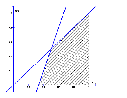
Figure 1: Allocation region.

What is the probability that the unit is allocated? To calculate that probability, we integrate over the shaded area in Figure 1:

$$1-F_{2}\left(\frac{1}{2}\right)+\int_{1/3}^{1/2}F_{3|x_{(2)}}(3x_{(2)}-1)f_{2}(x_{(2)}).$$ (16)

Recall that $F_{2}$ is the distribution of the second order statistic $X_{(2)}$ and $F_{3|x_{(2)}}$ is the distribution of $X_{(3)}$ conditional on $X_{(2)}=x_{(2)}.$ Here, $F_{2}(x)=3x^{2}-2x^{3},$ with density $f_{2}(x)=6x(1-x),$ and $F_{3|x_{(2)}}(x)=\frac{x}{x_{(2)}},$ with density $f_{3|x_{(2)}}(x)=\frac{1}{x_{(2)}}.$ Substituting these definitions into Expression 16, we find that the probability of allocation is $\frac{23}{36}\approx 0.64$.

Similarly, substituting $f_{2}$ and $f_{3|x_{(2)}}$ into Expression 14 gives the seller’s expected revenue:

$${\int_{1/3}^{1/2}\int_{0}^{3x_{(2)}-1}\left[3x_{(2)}-1-x_{(3)}\right]}\frac{1}{x_{(2)}}{6x_{(2)}(1-x_{(2)})}$$

$$+{\int_{1/2}^{1}\int_{0}^{x_{(2)}}\left[3x_{(2)}-1-x_{(3)}\right]\frac{1}{x_{(2)}}6x_{(2)}(1-x_{(2)}).}$$

Integrating these expressions yields expected revenue of $\frac{55}{144}\approx 0.382$. We can also compute the expected revenue to the second seller and find that it is $\frac{125}{432}\approx 0.289.$ By contrast, in the absence of any reserve rule, both sellers earn $E[X_{(3)}]=0.25$. Thus, the second seller also benefits when the first seller uses the optimal reserve rule.

4 The Optimal Mechanism when $r>\underline{x}$

We now consider the more general case where there may be a non-trivial reserve price in the second auction ($r>\underline{x}$). We find that whenever $r$ is below $\psi^{-1}(0)$, the optimal reserve price in the standard setting, then the optimal mechanism for the first seller is qualitatively very similar to what we found in the baseline case of $r=0$. Differences arise only when exactly one or two bidders have valuations above $r$, a scenario that is unlikely when $r$ is low or the number of bidders $N$ is large. When $r\geq\psi^{-1}(0)$, then a mechanism closer to a standard auction is optimal for the first seller.

Our analysis proceeds as follows. Now the payoff to a buyer $i$ with valuation $X_{i}\geq r$ in the second period, provided that he did not obtain the first object, depends not only on the seller’s allocation decision, but also on whether or not the highest and second highest types among his rivals exceed $r$. As a result, we have more cases to consider. The payoff to a buyer $i$ in the second period is

$$\max\{X_{i}-\max\left\{r,Y_{(2)}\right\},0\}$$

if the first object is allocated to the competitor with the highest type $Y_{(1)}$, and it is

$$\max\left\{X_{i}-\max\left\{r,Y_{(1)}\right\},0\right\}$$

otherwise. Thus, the expected payoff to a bidder $i$ with type $x_{i}\geq r$, given reports $\mathbf{x}$ and excluding any payment to the first seller, is

$$\begin{array}[]{c}P_{i}(\mathbf{x)}\cdot x_{i}+P_{j(1)}(\mathbf{x)}\cdot\max\left\{x_{i}-\max\left\{r,y_{(2)}\right\},0\right\}\\ +\left(1-P_{i}(\mathbf{x)}-P_{j(1)}(\mathbf{x)}\right)\cdot\max\left\{x_{i}-\max\left\{r,y_{(1)}\right\},0\right\},\end{array}$$

where as before $y_{(1)}$ and $y_{(2)}$ denote the two highest valuations among his competitors, $j(1)$ is the highest-type competitor (so that $X_{j(1)}=y_{(1)}$), and $P_{i}(\mathbf{x)}$ denotes the probability that the first object is assigned to buyer $i$ given $\mathbf{x.}$ The payoff to a buyer $i$ with type $x_{i}<r$ in the second period is 0, so the expected payoff given $\mathbf{x}$ is just $P_{i}(\mathbf{x)}\cdot x_{i}.$

Based on these payoffs, the interim expected payoff to a buyer of type $x\geq r$ when all buyers report truthfully, excluding any payment to the first seller, can be expressed as

$$\begin{array}[]{ccc}\Pi(x|x)&=&{\int\limits_{\left[\underline{x},\bar{x}\right]^{N-1}:r>\widehat{y}_{1}}}\left(x-r+\hat{p}^{1}\left(\left(x;\widehat{\mathbf{y}}\right)\right)\cdot r\right)\widehat{\mathbf{g}}(\widehat{\mathbf{y}})\\ &+&{\int\limits_{\left[\underline{x},\bar{x}\right]^{N-1}:x>\widehat{y}_{1}\geq r>\widehat{y}_{2}}}\left(x-\widehat{y}_{1}+\hat{p}^{1}\left(\left(x;\widehat{\mathbf{y}}\right)\right)\cdot\widehat{y}_{1}+\hat{p}^{2}\left(\left(x;\widehat{\mathbf{y}}\right)\right)\cdot\left[\widehat{y}_{1}-r\right]\right)\widehat{\mathbf{g}}(\widehat{\mathbf{y}})\\ &+&{\int\limits_{\left[\underline{x},\bar{x}\right]^{N-1}:x>\widehat{y}_{1}\geq\widehat{y}_{2}\geq r}}\left(x-\widehat{y}_{1}+\hat{p}^{1}\left(\left(x;\widehat{\mathbf{y}}\right)\right)\cdot\widehat{y}_{1}+\hat{p}^{2}\left(\left(x;\widehat{\mathbf{y}}\right)\right)\cdot\left[\widehat{y}_{1}-\widehat{y}_{2}\right]\right)\widehat{\mathbf{g}}(\widehat{\mathbf{y}})\\ &+&{\int\limits_{\left[\underline{x},\bar{x}\right]^{N-1}:\widehat{y}_{1}\geq x,r>\widehat{y}_{2}}}\left(\hat{p}^{1}\left(\left(x;\widehat{\mathbf{y}}\right)\right)\cdot\left[x-r\right]+\hat{p}^{2}\left(\left(x;\widehat{\mathbf{y}}\right)\right)\cdot x\right)\widehat{\mathbf{g}}(\widehat{\mathbf{y}})\\ &+&{\int\limits_{\left[\underline{x},\bar{x}\right]^{N-1}:\widehat{y}_{1}\geq x>\widehat{y}_{2}\geq r}}\left(\hat{p}^{1}\left(\left(x;\widehat{\mathbf{y}}\right)\right)\cdot\left[x-\widehat{y}_{2}\right]+\hat{p}^{2}\left(\left(x;\widehat{\mathbf{y}}\right)\right)\cdot x\right)\widehat{\mathbf{g}}(\widehat{\mathbf{y}})\\ &+&{\displaystyle\sum_{k=2}^{N-1}}\left[{\int\limits_{\left[\underline{x},\bar{x}\right]^{N-1}:\widehat{y}_{k}\geq x>\widehat{y}_{k+1}}}\left(\hat{p}^{k+1}\left(\left(x;\widehat{\mathbf{y}}\right)\right)\cdot x\right)\widehat{\mathbf{g}}(\widehat{\mathbf{y}})\right].\end{array}$$

The first three integral terms give the payoffs to the buyer when his type $x$ is the highest, the fourth and fifth integral terms are the payoffs when $x$ is the second highest type, and the last term is the payoff when $x$ is the $k$-th highest type, $k\geq 3$. In each of these terms, if the first good is allocated to the buyer, then his payoff is simply $x$. His payoff when he does not get the first good depends on the values of the highest and second-highest rival types and on whether or not the first good is allocated to one of them. The six possible cases, beginning with the first term, are as follows:

• If all rivals have values below the reserve price (i.e., $r>\widehat{y}_{1}$), then his continuation payoff is $x-r,$ regardless of whether or not the first good is allocated to a rival.

• If $x$ is the highest type, the highest rival type exceeds $r$, and all other rival types are below $r$ (i.e., $x>\widehat{y}_{1}\geq r>\widehat{y}_{2})$, then his continuation payoff is $x-r$ if the good is allocated to the highest rival and $x-\widehat{y}_{1}$ if not.

• If $x$ is the highest type and the two highest rival types both exceed $r$ (i.e., $x>\widehat{y}_{1}$ and $\widehat{y}_{2}\geq r)$, then his continuation payoff is $x-\widehat{y}_{2}$ if the good is allocated to the highest rival and $x-\widehat{y}_{1}$ if not.

• If the highest rival type exceeds $x$ and the second-highest rival type is less than $r$ (i.e., $\widehat{y}_{1}\geq x$ and $\widehat{y}_{2}<r)$, then his continuation payoff is $x-r$ if the good is allocated to the highest rival and $0$ if not.

• If $x$ lies between the highest and second highest rival types and the second-highest rival type exceeds $r$ (i.e., $\widehat{y}_{1}\geq x>\widehat{y}_{2}\geq r)$, then his continuation payoff is $x-\widehat{y}_{2}$ if the good is allocated to the highest rival and $0$ if not.

• If $x$ is less than the second-highest rival type (i.e., $\widehat{y}_{2}>x$), then he can never win the second object, so his continuation payoff is $0$.

A buyer of type $x<r$ is also never going to win the second auction. Therefore, his expected payoff from reporting truthfully is

$$\Pi(x|x) ={\int\limits_{\left[\underline{x},\bar{x}\right]^{N-1}:x>\widehat{y}_{1}}}\left(\hat{p}^{1}\left(\left(x;\widehat{\mathbf{y}}\right)\right)\cdot x\right)\widehat{\mathbf{g}}(\widehat{\mathbf{y}})$$

$$+{\displaystyle\sum_{k=1}^{N-1}}\left[{\int\limits_{\left[\underline{x},\bar{x}\right]^{N-1}:\widehat{y}_{k}\geq x>\widehat{y}_{k+1}}}\left(\hat{p}^{k+1}\left(\left(x;\widehat{\mathbf{y}}\right)\right)\cdot x\right)\widehat{\mathbf{g}}(\widehat{\mathbf{y}})\right].$$

Proceeding as in Section 3, we can show that the expected transfer to the seller from each bidder is

$$Et(\widehat{X}) =t(\underline{x})-\Pi(\underline{x}|\underline{x})$$ (17)

$$+\frac{1}{N}\left\{\begin{array}[]{cc}&{\int\limits_{\left[\underline{x},\bar{x}\right]^{N}:r>\widehat{x}_{1}}}\left(\hat{p}^{1}\left(\widehat{\mathbf{x}}\right)\cdot\psi(\widehat{x}_{1})\right)\mathbf{\hat{\mathbf{f}}}\left(\widehat{\mathbf{x}}\right)\\ +&{\int\limits_{\left[\underline{x},\bar{x}\right]^{N}:\widehat{x}_{1}\geq r>\widehat{x}_{2}}}\left(\psi(\widehat{x}_{1})-r+\hat{p}^{1}(\widehat{\mathbf{x}})\cdot r\right)\mathbf{\hat{\mathbf{f}}}\left(\widehat{\mathbf{x}}\right)\\ +&{\int\limits_{\left[\underline{x},\bar{x}\right]^{N}:\widehat{x}_{2}\geq r>\widehat{x}_{3}}}\left(\psi(\widehat{x}_{1})-\widehat{x}_{2}+\hat{p}^{1}(\widehat{\mathbf{x}})\cdot\widehat{x}_{2}+\hat{p}^{2}(\widehat{\mathbf{x}})\cdot\left[\widehat{x}_{2}-r\right]\right)\mathbf{\hat{\mathbf{f}}}\left(\widehat{\mathbf{x}}\right)\\ +&{\int\limits_{\left[\underline{x},\bar{x}\right]^{N}:\widehat{x}_{3}\geq r}}\left(\psi(\widehat{x}_{1})-\widehat{x}_{2}+\hat{p}^{1}(\widehat{\mathbf{x}})\cdot\widehat{x}_{2}+\hat{p}^{2}(\widehat{\mathbf{x}})\cdot\left[\widehat{x}_{2}-\widehat{x}_{3}\right]\right)\mathbf{\hat{\mathbf{f}}}\left(\widehat{\mathbf{x}}\right)\end{array}\right\}$$ (22)

$$+\frac{1}{N}\left\{\begin{array}[]{cc}&{\int\limits_{\left[\underline{x},\bar{x}\right]^{N}:r>\widehat{x}_{2}}}\left(\hat{p}^{2}\left(\widehat{\mathbf{x}}\right)\cdot\psi(\widehat{x}_{2})\right)\mathbf{\hat{\mathbf{f}}}\left(\widehat{\mathbf{x}}\right)\\ +&{\int\limits_{\left[\underline{x},\bar{x}\right]^{N}:\widehat{x}_{2}\geq r>\widehat{x}_{3}}}\left(\hat{p}^{1}(\widehat{\mathbf{x}})\cdot\left[\psi\left(\widehat{x}_{2}\right)-r\right]+\hat{p}^{2}(\widehat{\mathbf{x}})\cdot\psi\left(\widehat{x}_{2}\right)\right)\mathbf{\hat{\mathbf{f}}}\left(\widehat{\mathbf{x}}\right)\\ +&{\int\limits_{\left[\underline{x},\bar{x}\right]^{N}:\widehat{x}_{3}\geq r}}\left(\hat{p}^{1}(\widehat{\mathbf{x}})\cdot\left[\psi\left(\widehat{x}_{2}\right)-\widehat{x}_{3}\right]+\hat{p}^{2}(\widehat{\mathbf{x}})\cdot\psi\left(\widehat{x}_{2}\right)\right)\mathbf{\hat{\mathbf{f}}}\left(\widehat{\mathbf{x}}\right)\end{array}\right\}$$ (26)

$$+\frac{1}{N}\sum_{k=3}^{N}\int_{\left[\underline{x},\bar{x}\right]^{N}}\left(\hat{p}^{k}(\widehat{\mathbf{x}})\cdot\psi\left(\widehat{x}_{k}\right)\right)\mathbf{\hat{\mathbf{f}}}\left(\widehat{\mathbf{x}}\right).$$

The seller maximizes expected revenue $ER(\widehat{X})=N\cdot Et(\widehat{X})$ subject to incentive compatibility and individual rationality. Maximizing that integral pointwise, as we did in Section 3, yields a solution that may fail to be globally incentive compatible (a buyer may prefer to report a type far from his own), as we will see.

Given any vector of ordered types $\hat{\mathbf{x}}$, taking the derivative of the seller’s expected revenue with respect to $\hat{p}^{k}\left(\hat{\mathbf{x}}\right)$ yields the following:

1. If $\widehat{x}_{2}\geq r$,

   $$\frac{\partial ER(\widehat{X})}{\delta\hat{p}^{1}\left(\hat{\mathbf{x}}\right)}=\frac{\partial ER(\widehat{X})}{\delta\hat{p}^{2}\left(\hat{\mathbf{x}}\right)}=\left[\psi\left(\widehat{x}_{2}\right)+\widehat{x}_{2}-\max\left\{\widehat{x}_{3},r\right\}\right]\widehat{\mathbf{f}}(\widehat{\mathbf{x}}),$$

   and for all $k>2$,

   $$\frac{\partial ER(\widehat{X})}{\delta\hat{p}^{k}\left(\hat{\mathbf{x}}\right)}=\psi\left(\widehat{x}_{k}\right)\widehat{\mathbf{f}}(\widehat{\mathbf{x}}).$$

2. If $\widehat{x}_{1}\geq r>\widehat{x}_{2}$,

   $$\frac{\partial ER(\widehat{X})}{\delta\hat{p}^{1}\left(\hat{\mathbf{x}}\right)}=r\widehat{\mathbf{f}}(\widehat{\mathbf{x}})$$

   and for all $k>1$,

   $$\frac{\partial ER(\widehat{X})}{\delta\hat{p}^{k}\left(\hat{\mathbf{x}}\right)}=\psi\left(\widehat{x}_{k}\right)\widehat{\mathbf{f}}(\widehat{\mathbf{x}}).$$

3. If $r>\widehat{x}_{1}$, for all $k$,

   $$\frac{\partial ER(\widehat{X})}{\delta\hat{p}^{k}\left(\hat{\mathbf{x}}\right)}=\psi\left(\widehat{x}_{k}\right)\widehat{\mathbf{f}}(\widehat{\mathbf{x}}).$$

As before, global incentive compatibility is satisfied if a bidder cannot increase his probability of getting an item (either the first or the second) by underreporting his type, or decrease the probability by overreporting his type. We find that the solution to this pointwise maximization satisfies that condition when $r\in\left[\psi^{-1}(0),\bar{x}\right)$ but not when $r\in\left(\underline{x},\psi^{-1}(0)\right)$.

The source of the problem is a qualitative difference, relative to the no-reserve case, in the marginal revenue expression when $\widehat{x}_{1}\geq r>\widehat{x}_{2}$. If $\widehat{x}_{2}\geq r$, then the marginal revenue from allocating to the highest or second-highest bidder, $\psi\left(\widehat{x}_{2}\right)+\widehat{x}_{2}-\max\left\{\widehat{x}_{3},r\right\}$, matches what it was in the $r=0$ case: the only change is that $\max\left\{\widehat{x}_{3},r\right\}$ takes the place of $\widehat{x}_{3}$. If $\widehat{x}_{1}\geq r>\widehat{x}_{2}$, however, then the marginal revenue from allocating to the highest bidder is $r$, independent of the exact values of $\widehat{x}_{2}$ and $\widehat{x}_{3}$. As $\widehat{x}_{2}$ moves from just below $r$ to just above $r$, marginal revenue jumps from strictly positive to strictly negative. That downward switch drives the failure of global incentive compatibility, which we explore below.

4.1 If $r\in\left[\psi^{-1}(0),\bar{x}\right)$

Recall that when the first seller does not face competition from a second seller, then the optimal mechanism is to allocate the object to the bidder with the highest valuation if and only if $\psi(\widehat{x}_{1})\geq 0.$ Thus, if $r\in\left[\psi^{-1}(0),\bar{x}\right)$, then the second seller is using a reserve price higher than the optimal reserve price in the standard mechanism design setting. In this case, the solution to the first seller’s pointwise maximization problem is to

• allocate to the top bidder if $\widehat{x}_{1}\geq r>\widehat{x}_{2}$ or $r>\widehat{x}_{1}\geq\psi^{-1}(0)$, because the marginal revenue for $\hat{p}^{1}$ is $r>0$ or $\psi\left(\widehat{x}_{1}\right)>0$, respectively;

• allocate to one of the top two bidders if $\widehat{x}_{2}\geq r$, because the marginal revenue for both $\hat{p}^{1}$ and $\hat{p}^{2}$ is $\psi\left(\widehat{x}_{2}\right)+\widehat{x}_{2}-\max\left\{\widehat{x}_{3},r\right\}\geq\psi\left(\widehat{x}_{2}\right)>0;$

and not to allocate otherwise. If the seller uses this rule (and any method of breaking indifferences between allocating to the highest and second-highest bidders), then it is straightforward to show that the probability of getting an item (first or second) is increasing in the report. Thus, global incentive compatibility is satisfied.

Theorem 4

If the distribution of buyer values $F$ has increasing virtual values and the reserve price in the second auction is $r\in\left[\psi^{-1}(0),\bar{x}\right)$, then the following is an optimal (direct) mechanism for the first seller. (Ties are broken randomly.)

1. Allocation rule: The seller allocates the good if and only if $\psi\left(x_{(1)}\right)\geq 0;$ allocation in that case is to the bidder with the highest valuation if $x_{(2)}<r$, and it is to either the bidder with the highest valuation or the bidder with the second-highest valuation if $x_{(2)}\geq r$.

2. Transfers:

   1. If $\psi\left(x_{(1)}\right)\geq 0\text{ and }x_{(2)}<r$, then the bidder with the highest valuation pays $\max\left\{\psi^{-1}(0),x_{(2)}\right\}$ and the other bidders pay nothing.

   2. If $x_{(2)}\geq r$, then the bidder who receives the object pays $\max\left\{r,x_{(3)}\right\}$ and the other bidders pay nothing.

   3. If the good is not allocated, then there are no payments.

For brevity, we do not write out the expected revenues in Theorems 4, 6, and 7. It is straightforward to calculate those expected revenues from the specified transfer functions.

The mechanism in Theorem 4 can be implemented through a hybrid second- and third-price auction with reserve prices: if the highest bid is above $\psi^{-1}(0)$, then the item goes to the highest bidder at a price equal to either 1) the maximum of $\psi^{-1}(0)$ and the second-highest bid if that second-highest bid is below $r$, or 2) the maximum of $r$ and the third-highest bid if the second-highest bid is above $r$.

4.2 If $r\in\left(\underline{x},\psi^{-1}(0)\right)$

In this case, the second seller uses a reserve price lower than the optimal reserve price in the standard mechanism design setting, and the solution to the pointwise maximization problem turns out to violate incentive compatibility. Recall that for $r<\psi^{-1}(0)$, $a(r)\in\left[\underline{x},\bar{x}\right]$ is defined as the valuation that solves $a+\psi(a)=r.$ Note that $a(r)>r$ and $a(r)<\psi^{-1}(0)$. Given this definition, the solution to the pointwise maximization problem is to

• allocate to the top bidder if $\widehat{x}_{1}\geq r>\widehat{x}_{2}$;

• allocate to one of the top two bidders if $\widehat{x}_{3}\geq r$ and $\widehat{x}_{2}+\psi\left(\widehat{x}_{2}\right)-\widehat{x}_{3}\geq 0$;

• allocate to one of the top two bidders if $\widehat{x}_{2}\geq a(r)$ and $r>\widehat{x}_{3}$, because the marginal revenue for both $\hat{p}^{1}$ and $\hat{p}^{2}$ is $\widehat{x}_{2}+\psi\left(\widehat{x}_{2}\right)-r\geq a(r)+\psi\left(a(r)\right)-r=0;$

• not allocate if $a(r)>\widehat{x}_{2}$ and $r>\widehat{x}_{3}$, because the marginal revenue for both $\hat{p}^{1}$ and $\hat{p}^{2}$ is $\widehat{x}_{2}+\psi\left(\widehat{x}_{2}\right)-r<a(r)+\psi\left(a(r)\right)-r=0;$

and not to allocate otherwise.

This rule is not incentive compatible. To see why, suppose that bidder $i$ with type $x$ between $r$ and $a(r)$ considers deviating to a report $x^{\prime}$ below $r$. If $x$ is the highest type, then bidder $i$ is certain to get an item with either report: the first item if he reports $x$, the second item if he reports $x^{\prime}$. If $x$ is the third-highest or lower order type, then bidder $i$ will get nothing with either report. He will also get nothing if $x$ is the second-highest type and $\widehat{x}_{3}$ is greater than $r$, because the first unit will not be allocated at either report (the marginal revenue from doing so is negative), so bidder $i$ loses the second auction to the bidder with the highest type. The non-monotonicity arises when $x$ is the second-highest type and $\widehat{x}_{3}$ is less than $r$. If bidder $i$ reports truthfully, then the first unit is not allocated and he loses the second auction to the bidder with the highest type. But if he reports a type below $r,$ then the rule above specifies that the highest bidder gets the first unit, and then bidder $i$ will win the second. Thus, a bidder with a type between $r$ and $a(r)$ is more likely to get an item by reporting a type below $r$ than by reporting truthfully.

More formally, incentive compatibility requires the second-order condition that

$$\int_{q}^{x}\Pi_{2}(x^{\prime}|x^{\prime})dx^{\prime}\geq\int_{q}^{x}\Pi_{2}(q|x^{\prime})dx^{\prime},$$ (27)

for all $x,q\in\left[\underline{x},\bar{x}\right]$, where $\Pi_{2}(q|x)$, the derivative of the gross payoff $\Pi(q|x)$ with respect to the buyer’s true type, corresponds to the probability that buyer of type $x$ gets an item (either the first or the second) when reporting type $q$. (See Section 9.3.) The allocation rule derived above violates that condition at $x=r$ and any $q<r$.

We proceed to find the optimal mechanism through a process of “guess and verify.” First, we guess that the constraints in Expression 27 bind only for types $x$ below $a(r)$; that for type $r$ the constraint binds only for underreports $q<r$; and that for the rest of the types $x\leq a(r)$ the constraint binds only for a marginal underreport, $q=x-\epsilon$ for vanishingly small $\epsilon$. Those guesses yield a continuum of constraints that take the form

$$\int_{q}^{r}\Pi_{2}(x^{\prime}|x^{\prime})dx^{\prime}\geq\int_{q}^{r}\Pi_{2}(q|x^{\prime})dx^{\prime}$$ (28)

for each $q\in\left[\underline{x},r\right)$ (let $\lambda_{r,q}$ denote the corresponding Lagrange multiplier); and

$$\Pi_{2}(x|x)\geq\limsup_{\epsilon\searrow 0}\Pi_{2}(x-\epsilon|x)$$ (29)

for each $x\in\left(\underline{x},a(r)\right]$ (multiplier $\mu_{x}$). The constraints reflect the idea that a buyer must have a weakly higher chance of getting an object if he reports truthfully than if he underreports.

We derive first-order conditions by maximizing Expression 17 subject to the constraints in Expressions 28 and 29. We then guess the values of $\lambda_{r,q}$ and $\mu_{x}$, derive the solution using those guesses, and show that it satisfies incentive compatibility. (See Appendix 9.) The optimal mechanism corresponds to pointwise maximization except when there are either one or two bids above the reserve price $r$: the allocation rule is the same as in the no-reserve case when there are at least three bids above $r$, and it specifies no allocation when all bids are below $r$. When $\widehat{x}_{1}>r>$ $\widehat{x}_{3}$ and $\widehat{x}_{2}$ is either below $r$ or just above it (between $r$ and $a(r)$), then the constraints in Expressions 28 and 29 bind and the allocation rule needs to be adjusted. Depending on the value of $r$, the solution is to allocate either in all of these cases (regardless of the exact valuations of the bidders) or in none of them.

The intuition for this solution is as follows. We would like to allocate the good to the highest bidder when $\widehat{x}_{1}>r>\widehat{x}_{2}$, because the marginal revenue $r$ from doing so is positive, but not when $a(r)>\widehat{x}_{2}\geq r>\widehat{x}_{3}$, because in this case the marginal revenue is negative (i.e., $\widehat{x}_{2}+\psi\left(\widehat{x}_{2}\right)-r<0).$ Roughly, the constraints in Expression 28 mean that if we allocate when $\widehat{x}_{1}=x^{*}$ and $\widehat{x}_{2}<r$, then we also have to allocate when $\widehat{x}_{1}=x^{*}$ and $\widehat{x}_{2}=r$: otherwise a bidder with type $r$ would be more likely to get an item by underreporting. The constraints in Expression 29 then imply that we must also allocate when $\widehat{x}_{2}$ is just above $r$, and then when $\widehat{x}_{2}$ is just above that value, and so on. Iterating those constraints, we conclude that if we allocate when $\widehat{x}_{1}=x^{*}$ and $\widehat{x}_{2}<r$, then we must also allocate when we replace $\widehat{x}_{2}$ with any higher value, including values above $x^{*}$: that is, allocate whenever $\widehat{x}_{1}\geq x^{*}$.

The seller’s maximization problem, then, consists of finding the optimal cutoff $x^{*}$ such that when $\widehat{x}_{3}<r$ and $\widehat{x}_{2}<a(r)$, the seller allocates if and only if $\widehat{x}_{1}\geq x^{*}$. The resulting revenue is $N\cdot F\left(r\right)^{N-2}$ times $Z^{r}(x^{*})$, where the function $Z^{r}(x^{*})$ is defined as follows:

Definition 5

For $r\in\left[\underline{x},\bar{x}\right]$ and $x^{*}\in\left[r,\bar{x}\right]$, define

$$Z^{r}(x^{*})\equiv rF\left(r\right)\left[1-F\left(x^{*}\right)\right]+(N-1)\int\limits_{x^{*}}^{\bar{x}}\left(\int\limits_{r}^{\min\left\{x,a(r)\right\}}[\psi(x^{\prime})+x^{\prime}-r]f(x^{\prime})dx^{\prime}\right)f(x)dx.$$

To interpret $Z^{r}(x^{*})$, note that the revenue $N\cdot F\left(r\right)^{N-2}Z^{r}(x^{*})$ is the marginal revenue $r$ when $\widehat{x}_{1}\geq x^{*}$ and $\widehat{x}_{2}<r$ times the probability of that event, plus the (negative) expected marginal revenue when $\widehat{x}_{1}\geq x^{*}$ and $a(r)>\widehat{x}_{2}\geq r>\widehat{x}_{3}$ times the probability of that event. (Recall that when $\widehat{x}_{2}\geq a(r)$, we want to allocate regardless, so we do not need to include that case in the revenue maximization.) The function $Z^{r}(x^{*})$ is quasiconvex, so the optimal $x^{*}$ is at a corner: either $x^{*}=r$ or $x^{*}=\bar{x}$. Observe that $Z^{r}(\bar{x})=0$ (because $\widehat{x}_{1}$ cannot exceed $\bar{x}$). Thus, $x^{*}=\bar{x}$ is optimal if and only if $Z^{r}(r)\leq 0$, because then revenue is higher at $x^{*}=\bar{x}$ than at $x^{*}=r$. If $Z(r)\geq 0$, then $x^{*}=r$ is optimal. That logic forms the basis for our guesses of the values of the Lagrange multipliers.

The value of $Z^{r}(r)$ is decreasing in the number of bidders $N$. When $N$ is large enough, all else equal, the optimal cutoff $x^{*}$ equals $\bar{x}$, and the item is not allocated unless the second-highest bid is at least $a(r)$. We have not been able to establish whether or not $Z^{r}(r)$ is monotonic in the reserve price $r$. We do know, however, that for small enough values of $r$, again the optimal cutoff $x^{*}$ equals $\bar{x}$. The reason is that $Z^{r}(r)$ is continuous and strictly negative at $r=\underline{x}$. Thus, the optimal mechanism changes continuously near the baseline case of no reserve price in the second auction: for values of $r$ such that $Z^{r}(r)<0$, the seller allocates if and only if

$$\psi\left(\widehat{x}_{2}\right)+\widehat{x}_{2}-\max\left\{r,\widehat{x}_{3}\right\}\geq 0.$$ (30)

When $Z^{r}(r)>0$, then the seller allocates either if Condition 30 holds or if $\widehat{x}_{1}\geq r>\widehat{x}_{3}$.

We summarize the optimal mechanism in the following two theorems.

Theorem 6

If the distribution of buyer values $F$ has increasing virtual values, the reserve price in the second auction is $r\in\left(\underline{x},\psi^{-1}(0)\right)$, and $Z^{r}(r)\leq 0$, then the following is an optimal (direct) mechanism for the first seller. (Ties are broken randomly.)

1. Allocation rule: The seller allocates the good to the bidder with the second-highest valuation if $\psi\left(\widehat{x}_{2}\right)+\widehat{x}_{2}-\max\left\{r,\widehat{x}_{3}\right\}\geq 0,$ and does not allocate otherwise.

2. Transfers:

   1. If $x_{(3)}\leq r$ and the good is allocated ($x_{(2)}\geq a\left(r\right)$), then the bidder with the highest valuation pays $a\left(r\right)-r>0$, the bidder with the second-highest valuation pays $a\left(r\right)>0$, and the other bidders pay nothing.

   2. If $x_{(3)}\in\left(r,\psi^{-1}(0)\right)$ and the good is allocated ($x_{(2)}\geq a\left(x_{(3)}\right)$), then the bidder with the highest valuation pays $a\left(x_{(3)}\right)-x_{(3)}>0$, the bidder with the second-highest valuation pays $a\left(x_{(3)}\right)>0$, and the other bidders pay nothing.

   3. If $\psi\left(x_{(3)}\right)\geq 0$ (in which case the good is allocated because $x_{(2)}\geq a\left(x_{(3)}\right)=x_{(3)}$), then the bidder with the second-highest valuation pays $x_{(3)}>0$ and the other bidders pay nothing.

   4. If the good is not allocated, then there are no payments.

Theorem 7

If the distribution of buyer values $F$ has increasing virtual values, the reserve price in the second auction is $r\in\left(\underline{x},\psi^{-1}(0)\right)$, and $Z^{r}(r)\geq 0$, then the following is an optimal (direct) mechanism for the first seller. (Ties are broken randomly.)

1. Allocation rule: The seller allocates to the bidder with the highest valuation if $\widehat{x}_{1}\geq r>\widehat{x}_{2},$ allocates to either the bidder with the highest valuation or the bidder with the second-highest valuation if $\widehat{x}_{2}\geq r>\widehat{x}_{3},$ allocates to the bidder with the second-highest valuation if $\widehat{x}_{3}\geq r\text{ \emph{and }}\psi\left(\widehat{x}_{2}\right)+\widehat{x}_{2}-\widehat{x}_{3}\geq 0,$ and does not allocate otherwise.

2. Transfers:

   1. If $\widehat{x}_{1}\geq r>\widehat{x}_{2}$, then the bidder with the highest valuation pays $r$ and the other bidders pay nothing.

   2. If $\widehat{x}_{2}\geq r>\widehat{x}_{3}$, then the bidder who receives the object pays $r$ and the other bidders pay nothing.

   3. If $x_{(3)}\in\left(r,\psi^{-1}(0)\right)$ and the good is allocated ($x_{(2)}\geq a\left(x_{(3)}\right)$), then the bidder with the highest valuation pays $a\left(x_{(3)}\right)-x_{(3)}>0$, the bidder with the second-highest valuation pays $a\left(x_{(3)}\right)>0$, and the other bidders pay nothing.

   4. If $\psi\left(x_{(3)}\right)\geq 0$ (in which case the good is allocated because $x_{(2)}\geq a\left(x_{(3)}\right)=x_{(3)}$), then the bidder with the second-highest valuation pays $x_{(3)}>0$ and the other bidders pay nothing.

   5. If the good is not allocated, then there are no payments.

This mechanism is qualitatively similar to the optimal mechanism for the baseline case of no reserve price in the second auction, but it has some interesting new features. The optimal withholding rule now is a function of the first-, second-, and third-highest values, rather than just the second- and third-highest. Further, the withholding rule now varies with the number of bidders, unlike both our baseline case and the standard auction environment: as mentioned above, $Z^{r}(r)$ is decreasing in $N$.

5 Implementing the Optimal Mechanism

In this section, we show that the optimal mechanism can be implemented either with a modified third-price auction or with a modified pay-your-bid auction featuring a rebate. For simplicity, we focus on the case where there is no reserve price in the second auction ($r=0$), but the arguments extend to the case of a non-trivial $r$.

It is straightforward to implement the payments and allocation rule from Theorem 2 in a version of a third-price auction. Define the modified third-price auction as follows: each buyer submits a bid in $\left[\underline{x},\bar{x}\right]$. As a function of the vector of bids $\mathbf{b}$, the good is allocated to the second-highest bidder if and only if $b_{(2)}\geq a(b_{(3)}).$ If the unit is not allocated, then no one makes any payments. If the unit is allocated, then the payments are based on the third-highest bid, $b_{(3)}.$ When $\psi(b_{(3)})>0$, the highest bidder pays nothing and the second-highest bidder pays $b_{(3)}$; when $\psi(b_{(3)})<0$, then the highest bidder pays $a(b_{(3)})-b_{(3)}>0$ and the second-highest bidder pays $a(b_{(3)})$.

Theorem 8

If the distribution of buyer values $F$ has increasing virtual valuations, then truthful bidding is an equilibrium of the modified third-price auction, and that equilibrium yields the optimal expected revenue for the first seller.

In fact, truthful reporting is an ex post equilibrium. Consider, for example, the highest-valuation buyer in the case where $\psi(x_{(3)})<0$ and the item is allocated ($x_{(2)}\geq a(x_{(3)})$). Truthfully bidding $b=x_{(1)}$ yields a payoff of

$$x_{(1)}-x_{(3)}-\left[a(x_{(3)})-x_{(3)}\right]=x_{(1)}-a(x_{(3)});$$

the bidder transfers $a(x_{(3)})-x_{(3)})$ to the first seller and then wins the second auction at price $x_{(3)}$. Any bid above $x_{(2)}$ yields that same payoff. A bid between $a(x_{(3)})$ and $x_{(2)}$ also results in payoff $x_{(1)}-a(x_{(3)})$: the bidder gets the first item and transfers $a(x_{(3)})$ to the first seller. Any bid below $a(x_{(3)})$ gives a lower payoff, $x_{(1)}-x_{(2)}$, because the first item will not be allocated, no transfers will be made to the first seller, and the bidder will win the second item at price $x_{(2)}$. The other cases are similar.

Another way to implement the optimal mechanism is with a modified first-price or “pay your bid” auction, although the construction is more complicated. In Theorem 2, a bidder’s payment depends on whether his is the highest or second-highest bid, but he submits only a single bid. One solution is to implement the highest bidder’s transfer as an unconditional (i.e., regardless of whether or not the good is allocated) payment together with a rebate equal to the winning price in the second auction.

More formally, we show in Online Appendix A that a pay-your-bid auction with the following rules implements the optimal mechanism. A buyer with valuation $x$ submits a bid of $\beta(x)$. The seller allocates the object according to Expression 13, the rule from the optimal mechanism. It will turn out that $\beta(\cdot)$ is strictly increasing, so the seller can implement that rule. If the item is allocated, then both the highest and second-highest bidders pay their bids. If the item is not allocated, then only the highest bidder pays his bid. In either case, the highest bidder then gets a rebate equal to the sale price of the second item ($x_{(3)}$ if the first item is allocated, $x_{(2)}$ if it is not) assuming that he wins the second auction. The highest bidder does not get a rebate if he does not win the second auction.

6 Revenue Comparisons

In this section, we compare the expected revenue of the optimal mechanism to the expected revenue of a standard auction with an optimal reserve price. Relative to an optimal standard auction, how much better does the optimal mechanism with its more complicated reserve rule do? We show that the gains can be substantial. As in Section 5, for simplicity we study the case with no reserve price in the second auction ($r=0$). The first step is derive the symmetric equilibrium in the first auction with a positive reserve price, $r_{1}$. This derivation turns out to be a significant challenge, because the equilibrium involves pooling.

Proposition 9

When $r=0$, then for any $r_{1}\in(0,E[Y_{(1)}])$, there is no strictly increasing, symmetric pure-strategy equilibrium of either a first-price auction or a second-price auction with reserve price $r_{1}$ for the first good.

(If the reserve price $r_{1}$ exceeds $E[Y_{(1)}]$, the expectation of the highest rival value, then no one will submit a bid above the reserve price in the first auction.) To see the reasoning behind the non-existence result, consider a second-price auction with reserve price $r_{1}$ and suppose that there is a symmetric equilibrium with a strictly increasing bidding function $\beta$. The first-order condition for an optimal bid above $r_{1}$ gives

$$\beta(x)=E[Y_{(2)}|Y_{(1)}=x],$$ (31)

the expected price in the second auction conditional on losing the first auction to another bidder of type $x$. Let $\hat{x}\geq r_{1}$ denote the lowest valuation such that a buyer submits a bid. A buyer with valuation $\hat{x}$ must be indifferent between submitting a bid of $\beta(\hat{x})$ in the first auction and not submitting a bid. (If he strictly preferred to bid, then so would nearby types, and $\hat{x}$ would not be the lowest type to submit a bid.) The expected total payoff from submitting $\beta(\hat{x})$ is

$$(\hat{x}-r)G_{1}(\hat{x})+\int_{\hat{x}}^{\bar{x}}\left[\int_{\underline{x}}^{\hat{x}}[\hat{x}-y_{(2)}]g_{2|y_{(1)}}(y_{(2)})\right]g_{1}(y_{(1)});$$

the expected payoff from not submitting a bid is

$$\int_{\underline{x}}^{\hat{x}}[x-y_{(1)}]g_{1}(y_{(1)})+\int_{\hat{x}}^{\bar{x}}\left[\int_{\underline{x}}^{\hat{x}}[\hat{x}-y_{(2)}]g_{2|y_{(1)}}(y_{(2)})\right]g_{1}(y_{(1)}).$$

The difference is zero when

$$(\hat{x}-r_{1})G_{1}(\hat{x})=\int_{\underline{x}}^{\hat{x}}[x-y_{(1)}]g_{1}(y_{(1)})\Leftrightarrow r_{1}=\frac{1}{G_{1}(\hat{x})}\int_{\underline{x}}^{\hat{x}}y_{(1)}g_{1}(y_{(1)})=E[Y_{(1)}|Y_{(1)}\leq\hat{x}].$$

But that value of $r_{1}$ is strictly greater than the value of $\beta(\hat{x})$ from Expression 31. (The former is the expectation of the highest of $N-1$ valuations, conditional on all being below $\hat{x}$, while the latter is the expectation of the highest of $N-2$, again conditional on all being below $\hat{x}$.) Thus, these two necessary conditions for equilibrium are incompatible, and we conclude that no strictly increasing, symmetric equilibrium of the second-price auction with reserve price $r_{1}$ exists.

The non-existence result is not surprising. In our model, allocating the good in the first auction generates a positive externality for the losing buyers. Jehiel and Moldovanu [15] were the first to observe that a pure-strategy symmetric separating equilibrium does not exist in a second-price auction with positive externalities. However, they show that a symmetric equilibrium with partial pooling at the reserve price can exist. In that equilibrium, an interval of types $[\hat{x},\hat{\hat{x}}]$ all bid $r_{1}$, types above $\hat{\hat{x}}$ bid according to a strictly increasing $\beta(x)$, and types below $\hat{x}$ do not bid. We construct such an equilibrium for our example and then calculate the optimal reserve price and revenues for the first seller.

6.1 Three bidders, uniform valuations

We will derive the partial-pooling equilibrium of the second price auction with reserve $r_{1}$ for the $N=3$, $F=U[0,1]$, $r=0$ case and compute the optimal reserve price of the first seller and associated revenue. Details are in Online Appendix B. In the example, Expression 31 becomes $\beta(x)=x/2$. The cutoff values $\hat{x}$ and $\hat{\hat{x}}$ are characterized by two indifference conditions. A buyer of type $\hat{\hat{x}}$ is indifferent between bidding $r_{1}$ (and tying with other types in $[\hat{x},\hat{\hat{x}}]$) and bidding just above $r_{1}$; a buyer of type $\hat{x}$ is indifferent between bidding $r$ and not bidding. The type-$\hat{\hat{x}}$ buyer trades off overpaying for the first item relative to the expected price in the second auction when there is only one rival with a type in $[\hat{x},\hat{\hat{x}}]$ against underpaying when there are two such rivals. The type-$\hat{x}$ buyer overpays when there are 0 or 1 rival with type in $[\hat{x},\hat{\hat{x}}]$, but may get an item even when both rivals have higher types.

Solving the two indifference conditions gives $\hat{x}=(1+1/\sqrt{3})r_{1}$ and $\hat{\hat{x}}=(1+2/\sqrt{3})r_{1}$. We next find the optimal reserve price $r_{1}^{\ast}$ by maximizing the seller’s expected revenue $R_{1}(r_{1})$:

$$R_{1}(r_{1})=\left[F_{1}(\hat{\hat{x}})-F_{1}(\hat{x})\right]r_{1}+\int\limits_{\hat{\hat{x}}}^{1}\left[F_{2|x_{(1)}}(\hat{\hat{x}})r_{1}+\int\limits_{\hat{\hat{x}}}^{x_{(1)}}\beta(x_{(2)})f_{2|x_{(1)}}(x_{(2)})\right]f_{1}(x_{(1)}).$$

The solution is $r_{1}^{\ast}\approx 0.379$. The corresponding values of $\hat{x}$ and $\hat{\hat{x}}$ are $\hat{x}\approx 0.60$ and $\hat{\hat{x}}\approx 0.82$, and the resulting maximal revenue is $R_{1}(r_{1}^{\ast})\approx 0.303.$

The revenue of the second seller is the second-highest valuation $x_{(2)}$ if the first seller does not allocate and the third-highest valuation $x_{(3)}$ otherwise – except if all three valuations are between $\hat{x}$ and $\hat{\hat{x}}$ and the first seller randomly allocates to the buyer with valuation $x_{(3)}$, in which case the second seller gets $x_{(2)}$ instead of $x_{(3)}$. Overall, the expected revenue for the second seller when the first seller sets the optimal reserve price is $R_{2}(r_{1}^{\ast})\approx 0.282.$

A striking feature of this equilibrium is that the threshold for bidding, $\hat{x},$ is significantly higher than the optimal reserve price, $r_{1}^{\ast}$. The outside option of winning the second auction at a price below $r_{1}^{\ast}$ causes types between $r_{1}^{\ast}$ and $\hat{x}$ not to bid in the first auction. Their lack of participation gives the high types an incentive to participate because they are more likely to win the first auction at price equal to $r_{1}^{\ast}$. As a result, only 40% of the buyers bid in the first auction and roughly half of them bid the reserve price.

Table 1 summarizes the revenue results for our uniform example.

Table 1: Revenue Comparisons when $$r=0$$

First Seller Revenues Second Seller Revenues

Optimal Mechanism 0.382 0.289

Must-Sell Mechanism 0.250 0.250

Optimal Second Price Auction 0.303 0.282

    

In comparison to the must-sell mechanism, the optimal mechanism increases the expected revenues of both sellers, by 54% for the first seller and by 16% for the second seller. A standard auction with an optimal reserve price gives the second seller essentially the same increase but gives the first seller only a 20% increase in revenues.

Table 1 compares revenues only for the case where the second seller does not use a reserve price. However, the above analysis strongly suggests that reserve prices in standard auctions are not a very effective way for the first seller to increase revenues in a sequential auction setting.

7 Extensions

The design of the optimal mechanism can be straightforwardly extended to environments in which either or both sellers have multiple units. For example, suppose that the first seller has one unit to sell and the second seller has $M$ units that she sells simultaneously in a uniform-price auction with no reserve. Buyers have a weakly dominant strategy to bid their value in second period so there is no leakage problem. Then the optimal allocation rule is to allocate the unit to the $\left(M+1\right)$-th highest type if and only if $\psi(x_{(M+1)})+M(x_{(M+1)}-x_{(M+2)})>0$. The first term is the virtual valuation of the marginal buyer (the one who gets an object if the first seller allocates and not otherwise), and the second term is the total savings to the $M$ buyers from reducing the price in the second auction from $x_{\left(M+1\right)}$ to $x_{\left(M+2\right)}$.

More broadly, we hope that our analysis can be used as a framework for studying sequential competition in mechanisms between sellers, in a setting where the second seller also acts strategically in choosing her mechanism. Although in many real-world settings the relevant competition facing a seller comes from future auctions (or, equivalently, from a Bertrand market), we believe that such an extension would be valuable.For instance, the optimal response of the second seller may not be a second-price auction with a reserve price. When the first unit is allocated to the second-highest type, then the second seller faces a distribution of types that may not have increasing virtual valuations, even if the original distribution does. The inherited distribution is “hollowed out,” in the sense that a middle value is the one that gets removed. Further, the first seller’s optimal allocation rule implies that the types of the bidders remaining to face the second seller are correlated.

The spillover effect between sequential sellers that we have identified is conceptually distinct from the problem of information leakage, but the two issues may interact. In general, the best response for the second seller depends on what information about the bidders’ types is disclosed after the first period. Consider the extreme case (as in Carroll and Segal [12]) where all private information is exogenously revealed after the first mechanism is run. If the second seller has all the bargaining power, then she will make a take-it-or-leave-it offer to the highest-type remaining buyer at exactly his value. Since the buyers anticipate that they will get no surplus in the second period, the problem facing the first seller is equivalent to the standard mechanism design environment. On the other hand, if the buyers have all the bargaining power in the second period, then the remaining buyer with the highest value will get the second item at a price equal to the second-highest remaining value, and so our optimal mechanism emerges as the equilibrium choice for the first seller.

Information leakage may similarly complicate outcomes in the case of more than two sequential sellers, if buyers worry that information about their types revealed in their bids will influence the future bids of their competitors. One potential solution would be to restrict sellers to ex post incentive compatible mechanisms, in order to isolate the effects of sequential competition in mechanisms from those of information leakage.

8 Concluding Remarks

In sequential auction environments, losers of one auction can try to buy again, typically from a different seller. In this paper we show that for a seller who faces such competition from a subsequent auction, using a standard first- or second-price auction with a reserve price does not maximize revenue. Instead, we characterize the optimal mechanism for any given reserve price by the second seller, using techniques that may be useful in other settings where the first-order approach does not yield an incentive compatible solution. The optimal mechanism features payments from the top two bidders and a reserve rule that depends on the two or three highest valuations. We also present a third-price auction and a pay-your-bid auction with a rebate that can be used in practice to implement the optimal mechanism.

We formulate our model in terms of sale auctions, but we can equally interpret it as a model of procurement auctions, where the bidders are potential sellers and their types represent their production costs. An important motivating example is the market for pharmaceuticals in Ecuador and other middle-income countries, studied by Brugués [8]. There, the first buyer is the government, who procures a supply for the public market. Losing bidders compete to serve the private market, where Bertrand competition yields the same outcome as a second-price auction with no reserve. Our analysis may be especially relevant in this environment, because a government agency may have greater ability to implement non-standard auction rules than would a private seller.

Our setting is a special case of a mechanism design environment with externalities: when a bidder wins the first auction, then he will not compete in the second auction. His absence, if he has the highest or second-highest type, increases the continuation payoff (that is, the payoff from the second auction) for the bidder with the highest remaining type. We analyze how a seller can increase revenues or a buyer can reduce her procurement payments by accounting for this externality in the design of her auction.

We view our analysis as a first step in studying competition in mechanisms between sellers in a sequential setting. There are many ways of modeling such competition with regard to the timing of moves and information revelation. One interesting possibility is to assume that types are revealed after the first seller runs her auction (as is done in Bergemann et al. [6] and in Carroll and Segal [12]) and to model the second stage as a Nash bargaining game between the second seller and the remaining buyer with the highest value. The Nash bargaining solution breaks the tie between allocating to the highest or second-highest bidder in the optimal mechanism for the first seller – the surplus from allocating to the highest bidder strictly strictly exceeds the surplus from allocating to the second-highest bidder. As a result, the pointwise revenue maximizing solution may fail to be incentive compatible.

9 Appendix: Proving Theorems 4, 6, and 7

9.1 Payoff from false report

We derive the payoff to a type-$x$ buyer who reports his type as $q$. If $x\geq r$ and $q\geq x$, then

$$\begin{array}[]{ccc}\Pi(q|x)&=&{\int\limits_{\left[\underline{x},\bar{x}\right]^{N-1}:x>\widehat{y}_{1}}}\left(\begin{array}[]{c}x-\max\left\{\widehat{y}_{1},r\right\}+\hat{p}^{1}\left(\left(q;\widehat{\mathbf{y}}\right)\right)\cdot\max\left\{\widehat{y}_{1},r\right\}\\ +\hat{p}^{2}\left(\left(q;\widehat{\mathbf{y}}\right)\right)\cdot\left[\max\left\{\widehat{y}_{1},r\right\}-\max\left\{\widehat{y}_{2},r\right\}\right]\end{array}\right)\widehat{\mathbf{g}}(\widehat{\mathbf{y}})\\ &+&{\int\limits_{\left[\underline{x},\bar{x}\right]^{N-1}:q>\widehat{y}_{1}\geq x>\widehat{y}_{2}}}\left(\hat{p}^{1}\left(\left(q;\widehat{\mathbf{y}}\right)\right)\cdot x+\hat{p}^{2}\left(\left(q;\widehat{\mathbf{y}}\right)\right)\cdot\left[x-\max\left\{\widehat{y}_{2},r\right\}\right]\right)\widehat{\mathbf{g}}(\widehat{\mathbf{y}})\\ &+&{\int\limits_{\left[\underline{x},\bar{x}\right]^{N-1}:q>\widehat{y}_{1}>\widehat{y}_{2}\geq x}}\left(\hat{p}^{1}\left(\left(q;\widehat{\mathbf{y}}\right)\right)\cdot x\right)\widehat{\mathbf{g}}(\widehat{\mathbf{y}})\\ &+&{\int\limits_{\left[\underline{x},\bar{x}\right]^{N-1}:\widehat{y}_{1}\geq q\geq x>\widehat{y}_{2}}}\left(\hat{p}^{1}\left(\left(q;\widehat{\mathbf{y}}\right)\right)\cdot\left[x-\max\left\{\widehat{y}_{2},r\right\}\right]+\hat{p}^{2}\left(\left(q;\widehat{\mathbf{y}}\right)\right)\cdot x\right)\widehat{\mathbf{g}}(\widehat{\mathbf{y}})\\ &+&{\displaystyle\sum_{k=1}^{N-1}}\left[{\int\limits_{\left[\underline{x},\bar{x}\right]^{N-1}:\widehat{y}_{k}\geq q>\widehat{y}_{k+1},\widehat{y}_{2}\geq x}}\left(\hat{p}^{k+1}\left(\left(q;\widehat{\mathbf{y}}\right)\right)\cdot x\right)\widehat{\mathbf{g}}(\widehat{\mathbf{y}})\right].\end{array}$$

If $x\geq r$ and $q<x$, then

$$\begin{array}[]{ccc}\Pi(q|x)&=&{\int\limits_{\left[\underline{x},\bar{x}\right]^{N-1}:q>\widehat{y}_{1}}}\left(\begin{array}[]{c}x-\max\left\{\widehat{y}_{1},r\right\}+\hat{p}^{1}\left(\left(q;\widehat{\mathbf{y}}\right)\right)\cdot\max\left\{\widehat{y}_{1},r\right\}\\ +\hat{p}^{2}\left(\left(q;\widehat{\mathbf{y}}\right)\right)\cdot\left[\max\left\{\widehat{y}_{1},r\right\}-\max\left\{\widehat{y}_{2},r\right\}\right]\end{array}\right)\widehat{\mathbf{g}}(\widehat{\mathbf{y}})\\ &+&{\displaystyle\sum_{k=1}^{N-1}}\left[{\int\limits_{\left[\underline{x},\bar{x}\right]^{N-1}:\widehat{y}_{k}\geq q>\widehat{y}_{k+1},x>\widehat{y}_{1}}}\left(\begin{array}[]{c}x-\max\left\{\widehat{y}_{1},r\right\}\\ +\hat{p}^{1}\left(\left(q;\widehat{\mathbf{y}}\right)\right)\cdot\left[\max\left\{\widehat{y}_{1},r\right\}-\max\left\{\widehat{y}_{2},r\right\}\right]\\ +\hat{p}^{k+1}\left(\left(q;\widehat{\mathbf{y}}\right)\right)\cdot\max\left\{\widehat{y}_{1},r\right\}\end{array}\right)\widehat{\mathbf{g}}(\widehat{\mathbf{y}})\right]\\ &+&{\displaystyle\sum_{k=1}^{N-1}}\left[{\int\limits_{\left[\underline{x},\bar{x}\right]^{N-1}:\widehat{y}_{k}\geq q>\widehat{y}_{k+1},\widehat{y}_{1}\geq x>\widehat{y}_{2}}}\left(\begin{array}[]{c}\hat{p}^{1}\left(\left(q;\widehat{\mathbf{y}}\right)\right)\cdot\left[x-\max\left\{\widehat{y}_{2},r\right\}\right]\\ +\hat{p}^{k+1}\left(\left(q;\widehat{\mathbf{y}}\right)\right)\cdot x\end{array}\right)\widehat{\mathbf{g}}(\widehat{\mathbf{y}})\right]\\ &+&{\displaystyle\sum_{k=2}^{N-1}}\left[{\int\limits_{\left[\underline{x},\bar{x}\right]^{N-1}:\widehat{y}_{k}\geq q>\widehat{y}_{k+1},\widehat{y}_{2}\geq x}}\left(\hat{p}^{k+1}\left(\left(q;\widehat{\mathbf{y}}\right)\right)\cdot x\right)\widehat{\mathbf{g}}(\widehat{\mathbf{y}})\right].\end{array}$$

If $x<r$, then

$$\Pi(q|x)={\int\limits_{\left[\underline{x},\bar{x}\right]^{N-1}:q>\widehat{y}_{1}}}\left(\hat{p}^{1}\left(\left(q;\widehat{\mathbf{y}}\right)\right)\cdot x\right)\widehat{\mathbf{g}}(\widehat{\mathbf{y}})+{\displaystyle\sum_{k=1}^{N-1}}\left[{\int\limits_{\left[\underline{x},\bar{x}\right]^{N-1}:\widehat{y}_{k}\geq q>\widehat{y}_{k+1}}}\left(\hat{p}^{k+1}\left(\left(q;\widehat{\mathbf{y}}\right)\right)\cdot x\right)\widehat{\mathbf{g}}(\widehat{\mathbf{y}})\right].$$

9.1.1 $\Pi_{2}(q|x)$

The derivative of the payoff with respect to its second argument (the buyer’s true type), $\Pi_{2}(q|x)$, will be used below. If $x\geq r$ and $q\geq x$, then we calculate that derivative as

$$\begin{array}[]{ccc}\Pi_{2}(q|x)&=&{\int\limits_{\left[\underline{x},\bar{x}\right]^{N-1}:x>\widehat{y}_{1}}}\widehat{\mathbf{g}}(\widehat{\mathbf{y}})+{\int\limits_{\left[\underline{x},\bar{x}\right]^{N-1}:\widehat{y}_{1}\geq x>\widehat{y}_{2}}}\left(\hat{p}^{1}\left(\left(q;\widehat{\mathbf{y}}\right)\right)+\hat{p}^{2}\left(\left(q;\widehat{\mathbf{y}}\right)\right)\right)\widehat{\mathbf{g}}(\widehat{\mathbf{y}})\\ &+&{\int\limits_{\left[\underline{x},\bar{x}\right]^{N-1}:q>\widehat{y}_{1}>\widehat{y}_{2}\geq x}}\left(\hat{p}^{1}\left(\left(q;\widehat{\mathbf{y}}\right)\right)\right)\widehat{\mathbf{g}}(\widehat{\mathbf{y}})\\ &+&{\displaystyle\sum_{k=1}^{N-1}}\left[{\int\limits_{\left[\underline{x},\bar{x}\right]^{N-1}:\widehat{y}_{k}\geq q>\widehat{y}_{k+1},\widehat{y}_{2}\geq x}}\left(\hat{p}^{k+1}\left(\left(q;\widehat{\mathbf{y}}\right)\right)\right)\widehat{\mathbf{g}}(\widehat{\mathbf{y}})\right].\end{array}$$

If $x\geq r$ and $q<x$, then

$$\begin{array}[]{ccc}\Pi_{2}(q|x)&=&{\int\limits_{\left[\underline{x},\bar{x}\right]^{N-1}:x>\widehat{y}_{1}}}\widehat{\mathbf{g}}(\widehat{\mathbf{y}})+{\displaystyle\sum_{k=1}^{N-1}}\left[{\int\limits_{\left[\underline{x},\bar{x}\right]^{N-1}:\widehat{y}_{k}\geq q>\widehat{y}_{k+1},\widehat{y}_{1}\geq x>\widehat{y}_{2}}}\left(\begin{array}[]{c}\hat{p}^{1}\left(\left(q;\widehat{\mathbf{y}}\right)\right)\\ +\hat{p}^{k+1}\left(\left(q;\widehat{\mathbf{y}}\right)\right)\end{array}\right)\widehat{\mathbf{g}}(\widehat{\mathbf{y}})\right]\\ &+&{\displaystyle\sum_{k=2}^{N-1}}\left[{\int\limits_{\left[\underline{x},\bar{x}\right]^{N-1}:\widehat{y}_{k}\geq q>\widehat{y}_{k+1},\widehat{y}_{2}\geq x}}\left(\hat{p}^{k+1}\left(\left(q;\widehat{\mathbf{y}}\right)\right)\right)\widehat{\mathbf{g}}(\widehat{\mathbf{y}})\right].\end{array}$$

If $x<r$, then

$$\Pi_{2}(q|x)={\int\limits_{\left[\underline{x},\bar{x}\right]^{N-1}:q>\widehat{y}_{1}}}\left(\hat{p}^{1}\left(\left(q;\widehat{\mathbf{y}}\right)\right)\right)\widehat{\mathbf{g}}(\widehat{\mathbf{y}})+{\displaystyle\sum_{k=1}^{N-1}}\left[{\int\limits_{\left[\underline{x},\bar{x}\right]^{N-1}:\widehat{y}_{k}\geq q>\widehat{y}_{k+1}}}\left(\hat{p}^{k+1}\left(\left(q;\widehat{\mathbf{y}}\right)\right)\right)\widehat{\mathbf{g}}(\widehat{\mathbf{y}})\right].$$

9.2 Convexity

We show that the payoff $\Pi(q|x)$ is convex in its second argument (the buyer’s true type). The intuition is as follows: the derivative of $\Pi(q|x)$ with respect to the buyer’s type corresponds to the probability that the buyer gets an item (either the first or the second). Conditional on the report, that probability is increasing in the buyer’s type because a buyer with a higher valuation is more likely to win the second auction if he does not win the first item.

Formally, the second derivative of the payoff $\Pi(q|x)$ with respect to the buyer’s true type, $\Pi_{22}(q|x)$, when $x\geq r$ and $q\geq x$ is given by

$$\begin{array}[]{ccc}\Pi_{22}(q|x)&=&{\int\limits_{\left[\underline{x},\bar{x}\right]^{N-1}:\widehat{y}_{1}=x}}\left(1-\hat{p}^{1}\left(\left(q;\widehat{\mathbf{y}}\right)\right)-\hat{p}^{2}\left(\left(q;\widehat{\mathbf{y}}\right)\right)\right)\widehat{\mathbf{g}}(\widehat{\mathbf{y}})\\ &+&{\int\limits_{\left[\underline{x},\bar{x}\right]^{N-1}:q>\widehat{y}_{1},\widehat{y}_{2}=x}}\left(\hat{p}^{2}\left(\left(q;\widehat{\mathbf{y}}\right)\right)\right)\widehat{\mathbf{g}}(\widehat{\mathbf{y}})+{\int\limits_{\left[\underline{x},\bar{x}\right]^{N-1}:\widehat{y}_{1}\geq q,\widehat{y}_{2}=x}}\left(\hat{p}^{1}\left(\left(q;\widehat{\mathbf{y}}\right)\right)\right)\widehat{\mathbf{g}}(\widehat{\mathbf{y}}).\end{array}$$

The first integral represents the increase in the chance of getting an item when the buyer’s type moves from just below the highest competitor’s type $\widehat{y}_{1}$ to just above it: if $x>\widehat{y}_{1}$, then the buyer gets an item for sure because he would win the second auction. If $x<\widehat{y}_{1}$, then he gets an item only if he or the highest competitor gets the first item. Similarly, the second and third integrals represent the increase in the chance of getting an item when the buyer’s type moves from just below the second highest competitor’s type $\widehat{y}_{2}$ to just above it. Each of the three integrals is weakly positive, so $\Pi_{22}(q|x)\geq 0$.

Analogously, when $x\geq r$ and $q<x$, $\Pi_{22}(q|x)$ is given by

$$\begin{array}[]{ccc}\Pi_{22}(q|x)&=&{\displaystyle\sum_{k=1}^{N-1}}\left[{\int\limits_{\left[\underline{x},\bar{x}\right]^{N-1}:\widehat{y}_{k}\geq q>\widehat{y}_{k+1},\widehat{y}_{1}=x}}\left(1-\hat{p}^{1}\left(\left(q;\widehat{\mathbf{y}}\right)\right)-\hat{p}^{k+1}\left(\left(q;\widehat{\mathbf{y}}\right)\right)\right)\widehat{\mathbf{g}}(\widehat{\mathbf{y}})\right]\\ &+&{\displaystyle\sum_{k=2}^{N-1}}\left[{\int\limits_{\left[\underline{x},\bar{x}\right]^{N-1}:\widehat{y}_{k}\geq q>\widehat{y}_{k+1},\widehat{y}_{2}=x}}\left(\hat{p}^{1}\left(\left(q;\widehat{\mathbf{y}}\right)\right)\right)\widehat{\mathbf{g}}(\widehat{\mathbf{y}})\right]\geq 0.\end{array}$$

Finally, if $x<r$, then $\Pi_{22}(q|x)=0$: the buyer will never win the second auction, and his chance of getting the first item depends on his report but not his true type. Thus, $\Pi(q|x)$ is convex in the buyer’s valuation, as desired.

9.3 Incentive compatibility

Truthful reporting is a best response if and only if for all $x,q\in\left[\underline{x},\bar{x}\right]$,

$$U(x)=\Pi(x|x)-t(x)\geq(q|x)-t(q)=U(q)+\Pi(q|x)-\Pi(q|q)=U(q)+\intop_{q}^{x}\Pi_{2}(q|x^{\prime})dx^{\prime}.$$ (32)

By substituting (3) into (32), we can rewrite the incentive compatibility condition as

$$\int_{q}^{x}\Pi_{2}(x^{\prime}|x^{\prime})dx^{\prime}\geq\int_{q}^{x}\Pi_{2}(q|x^{\prime})dx^{\prime}.$$

That condition holds if for any type $x$ and any reports $q,q^{\prime}$ such that $q>x>q^{\prime}$, we have $\Pi_{2}(q|x)\geq\Pi_{2}(x|x)\geq\Pi_{2}(q^{\prime}|x)$. The allocation rules in Theorems 4, 6, and 7 have the property that $\hat{p}^{k}\left(\widehat{\mathbf{x}}\right)=0$ when $k>2$ for all $\widehat{\mathbf{x}}$, so the expressions for $\Pi_{2}(q|x)-\Pi_{2}(x|x)$ simplify. If $x\geq r$ and $q>x$, then

$$\begin{array}[]{cc}&\Pi_{2}(q|x)-\Pi_{2}(x|x)\\ =&{\int\limits_{\left[\underline{x},\bar{x}\right]^{N-1}:\widehat{y}_{1}\geq x>\widehat{y}_{2}}}\left(\hat{p}^{1}\left(\left(q;\widehat{\mathbf{y}}\right)\right)+\hat{p}^{2}\left(\left(q;\widehat{\mathbf{y}}\right)\right)-\hat{p}^{1}\left(\left(x;\widehat{\mathbf{y}}\right)\right)-\hat{p}^{2}\left(\left(x;\widehat{\mathbf{y}}\right)\right)\right)\widehat{\mathbf{g}}(\widehat{\mathbf{y}})\\ +&{\int\limits_{\left[\underline{x},\bar{x}\right]^{N-1}:q>\widehat{y}_{1}>\widehat{y}_{2}\geq x}}\left(\hat{p}^{1}\left(\left(q;\widehat{\mathbf{y}}\right)\right)\right)\widehat{\mathbf{g}}(\widehat{\mathbf{y}})+{\int\limits_{\left[\underline{x},\bar{x}\right]^{N-1}:\widehat{y}_{1}\geq q>\widehat{y}_{2}\geq x}}\left(\hat{p}^{2}\left(\left(q;\widehat{\mathbf{y}}\right)\right)\right)\widehat{\mathbf{g}}(\widehat{\mathbf{y}}).\end{array}$$ (33)

If $x\geq r$ and $q<x$, then

$$\begin{array}[]{cc}&\Pi_{2}(x|x)-\Pi_{2}(q|x)\\ =&{\int\limits_{\left[\underline{x},\bar{x}\right]^{N-1}:\widehat{y}_{1}\geq x>q>\widehat{y}_{2}}}\left(\hat{p}^{1}\left(\left(x;\widehat{\mathbf{y}}\right)\right)+\hat{p}^{2}\left(\left(x;\widehat{\mathbf{y}}\right)\right)-\hat{p}^{1}\left(\left(q;\widehat{\mathbf{y}}\right)\right)-\hat{p}^{2}\left(\left(q;\widehat{\mathbf{y}}\right)\right)\right)\widehat{\mathbf{g}}(\widehat{\mathbf{y}})\\ +&{\int\limits_{\left[\underline{x},\bar{x}\right]^{N-1}:\widehat{y}_{1}\geq x>\widehat{y}_{2}\geq q}}\left(\hat{p}^{1}\left(\left(x;\widehat{\mathbf{y}}\right)\right)+\hat{p}^{2}\left(\left(x;\widehat{\mathbf{y}}\right)\right)-\hat{p}^{1}\left(\left(q;\widehat{\mathbf{y}}\right)\right)\right)\widehat{\mathbf{g}}(\widehat{\mathbf{y}}).\end{array}$$ (34)

Because the allocation rules in Theorems 4, 6, and 7 have the property that $\hat{p}^{1}\left(\widehat{\mathbf{x}}\right)+\hat{p}^{2}\left(\widehat{\mathbf{x}}\right)$ is weakly increasing in $\widehat{x}_{1}$ and $\widehat{x}_{2}$, (33) and (34) are positive, as desired.

Next consider the case $x<r$. The allocation rules in Theorems 4, 6, and 7 have the additional property that $\hat{p}^{2}\left(\widehat{\mathbf{x}}\right)=0$ when $\widehat{x}_{2}<r$, so for $q>x$ we have

$$\begin{array}[]{cc}&\Pi_{2}(q|x)-\Pi_{2}(x|x)\\ =&{\int\limits_{\left[\underline{x},\bar{x}\right]^{N-1}:x>\widehat{y}_{1}}}\left(\hat{p}^{1}\left(\left(q;\widehat{\mathbf{y}}\right)\right)-\hat{p}^{1}\left(\left(x;\widehat{\mathbf{y}}\right)\right)\right)\widehat{\mathbf{g}}(\widehat{\mathbf{y}})\\ +&{\int\limits_{\left[\underline{x},\bar{x}\right]^{N-1}:q>\widehat{y}_{1}\geq x}}\left(\hat{p}^{1}\left(\left(q;\widehat{\mathbf{y}}\right)\right)\right)\widehat{\mathbf{g}}(\widehat{\mathbf{y}})+{\int\limits_{\left[\underline{x},\bar{x}\right]^{N-1}:\widehat{y}_{1}\geq q}}\left(\hat{p}^{2}\left(\left(q;\widehat{\mathbf{y}}\right)\right)\right)\widehat{\mathbf{g}}(\widehat{\mathbf{y}}).\end{array}$$ (35)

Finally, if $x<r$ and $q<x$, then

$$\begin{array}[]{cc}&\Pi_{2}(x|x)-\Pi_{2}(q|x)\\ =&{\int\limits_{\left[\underline{x},\bar{x}\right]^{N-1}:q>\widehat{y}_{1}}}\left(\hat{p}^{1}\left(\left(x;\widehat{\mathbf{y}}\right)\right)-\hat{p}^{1}\left(\left(q;\widehat{\mathbf{y}}\right)\right)\right)\widehat{\mathbf{g}}(\widehat{\mathbf{y}})+{\int\limits_{\left[\underline{x},\bar{x}\right]^{N-1}:x>\widehat{y}_{1}\geq q}}\left(\hat{p}^{1}\left(\left(x;\widehat{\mathbf{y}}\right)\right)\right)\widehat{\mathbf{g}}(\widehat{\mathbf{y}}).\end{array}$$ (36)

Because the specified allocation rules have the property that $\hat{p}^{1}\left(\widehat{\mathbf{x}}\right)$ is weakly increasing in $\widehat{x}_{1}$, (35) and (36) are both positive as well. We conclude that the mechanisms in Theorems 4, 6, and 7 are incentive compatible. It remains only to show that the allocation rules solve the seller’s revenue maximization problem. We made that argument for the $r\leq\underline{x}$ case in Section 3 and for the $r\in\left[\psi^{-1}(0),\bar{x}\right)$ case in Section 4.1. We cover the other cases next.

9.4 Constrained Optimization when $r\in\left(\underline{x},\psi^{-1}(0)\right)$

Recall that the seller’s problem is to maximize (17) subject to $\int_{q}^{r}\left[\Pi_{2}(x^{\prime}|x^{\prime})-\Pi_{2}(q|x^{\prime})\right]dx^{\prime}\geq 0$ for each $q\in\left[\underline{x},r\right)$ (with Lagrange multiplier $\lambda_{r,q}$), and to

$$\Pi_{2}(x|x)-\limsup_{\epsilon\searrow 0}\Pi_{2}(x-\epsilon|x)\geq 0$$

for each $x\in\left(\underline{x},a(r)\right]$ (multiplier $\mu_{x}$). Using the derivations in Section 9.1.1, we write out

$$\begin{array}[]{c}\Pi_{2}(x|x)-\limsup_{\epsilon\searrow 0}\Pi_{2}(x-\epsilon|x)=\\ \limsup_{\epsilon\searrow 0}\left\{\begin{array}[]{cc}&{\int\limits_{\left[\underline{x},\bar{x}\right]^{N-1}:x>\widehat{y}_{1}}}\left[\hat{p}^{1}\left(\left(x;\widehat{\mathbf{y}}\right)\right)-\hat{p}^{1}\left(\left(x-\epsilon;\widehat{\mathbf{y}}\right)\right)\right]\widehat{\mathbf{g}}(\widehat{\mathbf{y}})\\ +&\sum_{k=1}^{N-1}\left[\int_{\left[\underline{x},\bar{x}\right]^{N-1}:\widehat{y}_{k}\geq x>\widehat{y}_{k+1}}\left[\hat{p}^{k+1}\left(\left(x;\widehat{\mathbf{y}}\right)\right)-\hat{p}^{k+1}\left(\left(x-\epsilon;\widehat{\mathbf{y}}\right)\right)\right]\widehat{\mathbf{g}}(\widehat{\mathbf{y}})\right]\end{array}\right\}\end{array}$$

for each $x\in\left[\underline{x},r\right)$;

$$\begin{array}[]{c}\Pi_{2}(x|x)-\limsup_{\epsilon\searrow 0}\Pi_{2}(x-\epsilon|x)=\\ \limsup_{\epsilon\searrow 0}\left\{\begin{array}[]{cc}&{\int\limits_{\left[\underline{x},\bar{x}\right]^{N-1}:\widehat{y}_{1}\geq x>\widehat{y}_{2}}}\left[\begin{array}[]{c}\left(\hat{p}^{1}\left(\left(x;\widehat{\mathbf{y}}\right)\right)-\hat{p}^{1}\left(\left(x-\epsilon;\widehat{\mathbf{y}}\right)\right)\right)\\ +\left(\hat{p}^{2}\left(\left(x;\widehat{\mathbf{y}}\right)\right)-\hat{p}^{2}\left(\left(x-\epsilon;\widehat{\mathbf{y}}\right)\right)\right)\end{array}\right]\widehat{\mathbf{g}}(\widehat{\mathbf{y}})\\ +&\sum_{k=2}^{N-1}\left[\int_{\left[\underline{x},\bar{x}\right]^{N-1}:\widehat{y}_{k}\geq x>\widehat{y}_{k+1}}\left(\hat{p}^{k+1}\left(\left(x;\widehat{\mathbf{y}}\right)\right)-\hat{p}^{k+1}\left(\left(x-\epsilon;\widehat{\mathbf{y}}\right)\right)\right)\widehat{\mathbf{g}}(\widehat{\mathbf{y}})\right]\end{array}\right\}\end{array}$$

for each $x\in\left[r,a(r)\right]$;

$$\begin{array}[]{c}\Pi_{2}(r|r)-\Pi_{2}(q|r)=\\ \begin{array}[]{cc}&\begin{array}[]{cc}&\int_{\left[\underline{x},\bar{x}\right]^{N-1}:\widehat{y}_{1}\geq r>\widehat{y}_{2}}\left(\hat{p}^{1}\left(\left(r;\widehat{\mathbf{y}}\right)\right)+\hat{p}^{2}\left(\left(r;\widehat{\mathbf{y}}\right)\right)\right)\widehat{\mathbf{g}}(\widehat{\mathbf{y}})\\ +&\sum_{k=2}^{N-1}\left[\int_{\left[\underline{x},\bar{x}\right]^{N-1}:\widehat{y}_{k}\geq r>\widehat{y}_{k+1}}\hat{p}^{k+1}\left(\left(r;\widehat{\mathbf{y}}\right)\right)\widehat{\mathbf{g}}(\widehat{\mathbf{y}})\right]\end{array}\\ -&\left[\begin{array}[]{cc}&\int_{\left[\underline{x},\bar{x}\right]^{N-1}:\widehat{y}_{1}\geq r,\widehat{y}_{2}<q}\left(\hat{p}^{1}\left(\left(q;\widehat{\mathbf{y}}\right)\right)+\hat{p}^{2}\left(\left(q;\widehat{\mathbf{y}}\right)\right)\right)\widehat{\mathbf{g}}(\widehat{\mathbf{y}})\\ +&\sum_{k=1}^{N-1}\left[\int_{\left[\underline{x},\bar{x}\right]^{N-1}:\widehat{y}_{1}\geq r,\widehat{y}_{2}<r,\widehat{y}_{k}\geq q>\widehat{y}_{k+1}}\left(\begin{array}[]{c}\hat{p}^{1}\left(\left(q;\widehat{\mathbf{y}}\right)\right)\\ +\hat{p}^{k+1}\left(\left(q;\widehat{\mathbf{y}}\right)\right)\end{array}\right)\widehat{\mathbf{g}}(\widehat{\mathbf{y}})\right]\\ +&\sum_{k=2}^{N-1}\left[\int_{\left[\underline{x},\bar{x}\right]^{N-1}:\widehat{y}_{2}\geq r,\widehat{y}_{k}\geq q>\widehat{y}_{k+1}}\hat{p}^{k+1}\left(\left(q;\widehat{\mathbf{y}}\right)\right)\widehat{\mathbf{g}}(\widehat{\mathbf{y}})\right]\end{array}\right]\end{array}\end{array}$$

for each $q\in\left[\underline{x},r\right)$; and

$$\begin{array}[]{c}\Pi_{2}(x|x)-\Pi_{2}(q|x)=\\ \begin{array}[]{cc}&\begin{array}[]{cc}&{\int\limits_{\left[\underline{x},\bar{x}\right]^{N-1}:x>\widehat{y}_{1}}}\left(\hat{p}^{1}\left(\left(x;\widehat{\mathbf{y}}\right)\right)\right)\widehat{\mathbf{g}}(\widehat{\mathbf{y}})\\ +&{\displaystyle\sum_{k=1}^{N-1}}\left[{\int\limits_{\left[\underline{x},\bar{x}\right]^{N-1}:\widehat{y}_{k}\geq x>\widehat{y}_{k+1}}}\hat{p}^{k+1}\left(\left(x;\widehat{\mathbf{y}}\right)\right)\widehat{\mathbf{g}}(\widehat{\mathbf{y}})\right]\end{array}\\ -&\left[\begin{array}[]{cc}&{\int\limits_{\left[\underline{x},\bar{x}\right]^{N-1}:q>\widehat{y}_{1}}}\left(\hat{p}^{1}\left(\left(q;\widehat{\mathbf{y}}\right)\right)\right)\widehat{\mathbf{g}}(\widehat{\mathbf{y}})\\ +&{\displaystyle\sum_{k=1}^{N-1}}\left[{\int\limits_{\left[\underline{x},\bar{x}\right]^{N-1}:\widehat{y}_{k}\geq q>\widehat{y}_{k+1}}}\hat{p}^{k+1}\left(\left(q;\widehat{\mathbf{y}}\right)\right)\widehat{\mathbf{g}}(\widehat{\mathbf{y}})\right]\end{array}\right]\end{array}\end{array}$$

for each $x\in\left[\underline{x},r\right)$ and $q\in\left[\underline{x},x\right)$. Note that for $x\geq r$, the integrals do not include the case $x>\widehat{y}_{1}$, because the highest-type buyer is sure to get an object when his type is above $r$.

9.4.1 When $Z^{r}(r)\geq 0$

In this case, Theorem 7 specifies allocation whenever either i) $\widehat{x}_{1}\geq r>\widehat{x}_{3}$, or ii) $\widehat{x}_{3}\geq r$ and $\psi\left(\widehat{x}_{2}\right)+\widehat{x}_{2}-\widehat{x}_{3}\geq 0$, and not otherwise. We make the following guesses for the values of the Lagrange multipliers: for all $x\in\left[\underline{x},r\right)$, $\lambda_{r,x}=\mu_{x}=0;$ and for $x\in\left[r,a(r)\right]$, $\begin{array}[]{c}\mu_{x}=\int_{x}^{a(r)}N\cdot\left[r-x^{\prime}-\psi(x^{\prime})\right]f(x^{\prime})dx^{\prime}.\end{array}$ That is, only the immediate downward constraints for type $r$ and above bind. The intuition behind that guess for the values of $\mu_{x}$ is as follows: suppose that we relaxed the constraint that type $x\in\left[r,a(r)\right]$ must have a weakly higher chance of getting an object if he reports truthfully than if he underreports to $x-\epsilon$. Then the seller could not allocate when $\widehat{x}_{2}=x$ and $\widehat{x}_{3}<r$, and thus avoid earning the negative marginal revenue $x+\psi(x)-r$ in that case. There is an additional benefit: for type $x+\epsilon$, now underreporting does not lead to allocation, and so the seller is free to not allocate when $\widehat{x}_{2}=x+\epsilon$ and $\widehat{x}_{3}<r$, without violating the constraint for type $x+\epsilon$. Iterating, we see that relaxing the constraint for the single type $x$ allows the seller to avoid the negative marginal revenue $x^{\prime}+\psi(x^{\prime})-r$ for every type $x^{\prime}$ between $x$ and $a(r)$.

In what follows, the key feature of $\mu_{x}$ is that $\mu_{x}-\mu_{x+0}=N\cdot\left[r-x-\psi(x)\right]f(x)dx.$ For example, suppose that $\widehat{x}_{2}\in\left[r,a(r)\right)$. Allocating to either of the top two bidders in that case helps with the constraint for type $\widehat{x}_{2}$ (he gets an item by telling the truth), but it hurts with the constraint for a slightly higher type (he could get an item by underreporting his type as $\widehat{x}_{2}$). The net marginal effect is the difference between $\mu_{\widehat{x}_{2}}$ and $\mu_{\widehat{x}_{2}+0}$.

We use that key feature repeatedly as we next take the partial derivative of the seller’s expected revenue with respect to $\hat{p}^{k}\left(\hat{\mathbf{x}}\right)$, given any vector of ordered types $\hat{\mathbf{x}}$, and plug in those guesses. Note that for any $\widehat{\mathbf{x}}$ and any $k$, $N\cdot f(\widehat{x}_{k})\cdot\hat{\mathbf{g}}(\widehat{\mathbf{x}}_{-k})=\hat{\mathbf{f}}(\widehat{\mathbf{x}})$.

1. If $\widehat{x}_{2}\geq a(r)$, then $\frac{\partial ER(\widehat{X})}{\delta\hat{p}^{1}\left(\hat{\mathbf{x}}\right)}=\frac{\partial ER(\widehat{X})}{\delta\hat{p}^{2}\left(\hat{\mathbf{x}}\right)}=\left[\widehat{x}_{2}+\psi\left(\widehat{x}_{2}\right)-\max\left\{\widehat{x}_{3},r\right\}\right]\hat{\mathbf{f}}(\widehat{\mathbf{x}}).$

2. If $\widehat{x}_{2}\in\left[r,a(r)\right)$, then

   $$\frac{\partial ER(\widehat{X})}{\delta\hat{p}^{1}\left(\hat{\mathbf{x}}\right)}=\frac{\partial ER(\widehat{X})}{\delta\hat{p}^{2}\left(\hat{\mathbf{x}}\right)} =\left[\widehat{x}_{2}+\psi\left(\widehat{x}_{2}\right)-\max\left\{\widehat{x}_{3},r\right\}\right]\hat{\mathbf{f}}(\widehat{\mathbf{x}})+\hat{\mathbf{g}}(\widehat{\mathbf{x}}_{-2})\mu_{\widehat{x}_{2}}-\hat{\mathbf{g}}(\widehat{\mathbf{x}}_{-2})\mu_{\widehat{x}_{2}+0}$$

   $$=\left[\widehat{x}_{2}+\psi\left(\widehat{x}_{2}\right)-\max\left\{\widehat{x}_{3},r\right\}\right]\hat{\mathbf{f}}(\widehat{\mathbf{x}})$$

   $$+\hat{\mathbf{g}}(\widehat{\mathbf{x}}_{-2})N\cdot\left[r-\widehat{x}_{2}-\psi(\widehat{x}_{2})\right]f(\widehat{x}_{2})$$

   $$=\hat{\mathbf{f}}(\widehat{\mathbf{x}})\cdot\left[\widehat{x}_{2}+\psi\left(\widehat{x}_{2}\right)-\max\left\{\widehat{x}_{3},r\right\}+\left(r-\widehat{x}_{2}-\psi(\widehat{x}_{2})\right)\right]$$

   $$=\hat{\mathbf{f}}(\widehat{\mathbf{x}})\cdot\left[r-\max\left\{\widehat{x}_{3},r\right\}\right].$$

3. If $\widehat{x}_{1}\geq r$ and $\widehat{x}_{2}<r$, then $\frac{\partial ER(\widehat{X})}{\delta\hat{p}^{1}\left(\hat{\mathbf{x}}\right)}=r\hat{\mathbf{f}}(\widehat{\mathbf{x}})>0.$

4. In every case above, for all $k>2$ such that $\widehat{x}_{k}\geq a(r)$,

   $$\frac{\partial ER(\widehat{X})}{\delta\hat{p}^{k}\left(\hat{\mathbf{x}}\right)}=\psi\left(\widehat{x}_{k}\right)\hat{\mathbf{f}}(\widehat{\mathbf{x}})\leq\frac{\partial ER(\widehat{X})}{\delta\hat{p}^{2}\left(\hat{\mathbf{x}}\right)};$$

   for all $k>2$ such that $\widehat{x}_{k}\in\left[r,a(r)\right)$,

   $$\frac{\partial ER(\widehat{X})}{\delta\hat{p}^{k}\left(\hat{\mathbf{x}}\right)} =\psi\left(\widehat{x}_{k}\right)\hat{\mathbf{f}}(\widehat{\mathbf{x}})+\hat{\mathbf{g}}(\widehat{\mathbf{x}}_{-k})\mu_{\widehat{x}_{k}}-\hat{\mathbf{g}}(\widehat{\mathbf{x}}_{-k})\mu_{\widehat{x}_{k}+0}$$

   $$=\psi\left(\widehat{x}_{k}\right)\hat{\mathbf{f}}(\widehat{\mathbf{x}})+\hat{\mathbf{g}}(\widehat{\mathbf{x}}_{-k})N\cdot\left[r-\widehat{x}_{k}-\psi(\widehat{x}_{k})\right]f(\widehat{x}_{k})$$

   $$=\hat{\mathbf{f}}(\widehat{\mathbf{x}})\cdot\left[\psi\left(\widehat{x}_{k}\right)+\left(r-\widehat{x}_{k}-\psi(\widehat{x}_{k})\right)\right]=\hat{\mathbf{f}}(\widehat{\mathbf{x}})\cdot\left[r-\widehat{x}_{k}\right]<0;$$

   and for all $k$ such that $\widehat{x}_{k}<r$, $\frac{\partial ER(\widehat{X})}{\delta\hat{p}^{k}\left(\hat{\mathbf{x}}\right)}=\psi\left(\widehat{x}_{k}\right)\hat{\mathbf{f}}(\widehat{\mathbf{x}})<0.$

The marginal revenues above are weakly positive in each case where Theorem 7 specifies allocation, and they are weakly negative in each case where Theorem 7 specifies no allocation. Thus, our guesses for the values of the Lagrange multipliers, together with the allocation rule in Theorem 7, form a solution to the seller’s constrained optimization problem.

9.4.2 When $Z^{r}(r)\leq 0$

In this case, Theorem 6 specifies allocation if and only if $\psi\left(\widehat{x}_{2}\right)+\widehat{x}_{2}-\max\left\{r,\widehat{x}_{3}\right\}\geq 0$. The derivative of $Z^{r}(x^{*})$ is given by $z^{r}\left(x^{*}\right)f\left(x^{*}\right)$, where the function $z^{r}\left(x^{*}\right)$ is defined as

$$z^{r}(x^{*})\equiv-rF\left(r\right)+(N-1)\int\limits_{r}^{\min\left\{x^{*},a(r)\right\}}[r-x^{\prime}-\psi(x^{\prime})]f(x^{\prime})dx^{\prime}.$$

The function $z^{r}\left(x^{*}\right)$ is strictly increasing for $x^{*}<a(r)$ and constant for $x^{*}\geq a(r)$. When $Z^{r}\left(\bar{x}\right)-Z^{r}(r)=0-Z^{r}(r)\geq 0$, therefore, it must be that $z^{r}\left(a(r)\right)\geq 0$: otherwise $Z^{r}(x^{*})$ would be strictly decreasing throughout. We will use the inequality $z^{r}\left(a(r)\right)\geq 0$ below.

We make the following guesses for the Lagrange multipliers: for $x\in\left[\underline{x},r\right)$, $\begin{array}[]{c}\lambda_{r,x}=r\frac{N}{N-1}f\left(x\right)\end{array}$ and $\begin{array}[]{c}\mu_{x}=\int_{\underline{x}}^{x}r\frac{N}{N-1}F(x^{\prime})dx^{\prime};\end{array}$and for $x\in\left(r,a(r)\right]$, $\begin{array}[]{c}\mu_{x}=\int_{x}^{a(r)}N\cdot\left[r-x^{\prime}-\psi(x^{\prime})\right]f(x^{\prime})dx^{\prime}.\end{array}$ The differences relative to the $Z^{r}(r)\geq 0$ case are that now all the downward constraints bind for type $r$, and the immediate downward constraints bind for types below $r$. Allocating to either of the top two bidders when $\widehat{x}_{2}=r$ helps with all the downward constraints for type $r$, because he gets an item by telling the truth. On the other hand, allocating to the highest bidder when $\widehat{x}_{1}\geq r>\widehat{x}_{2}$ hurts with a constraint, because a bidder with type $r$ gets an object by underreporting his type as $\widehat{x}_{2}$. The intuition for our guess of the value of $\lambda_{r,x}$ is that if we relaxed the constraint, then the seller could allocate to the high bidder whenever $\widehat{x}_{1}\geq r>\widehat{x}_{2}$ and earn the corresponding marginal revenue $r$.

As we take the partial derivative of the seller’s expected revenue with respect to $\hat{p}^{k}\left(\hat{\mathbf{x}}\right)$ and plug in those guesses, we again use the feature that $\mu_{x}-\mu_{x+0}=N\cdot\left[r-x-\psi(x)\right]f(x)dx$ for $x\in\left(r,a(r)\right]$. Similarly, we use the feature that for $x\in\left[\underline{x},r\right)$, $\mu_{x+0}-\mu_{x}=r\frac{N}{N-1}F(x)dx.$

1. If $\widehat{x}_{2}\geq a(r)$, then

   $$\frac{\partial ER(\widehat{X})}{\delta\hat{p}^{1}\left(\hat{\mathbf{x}}\right)}=\left[\widehat{x}_{2}+\psi\left(\widehat{x}_{2}\right)-\max\left\{\widehat{x}_{3},r\right\}\right]\hat{\mathbf{f}}(\widehat{\mathbf{x}})-\sum_{k:\widehat{x}_{k}<r}\left[\hat{\mathbf{g}}(\widehat{\mathbf{x}}_{-k})\lambda_{r,\widehat{x}_{k}}\right]\leq\frac{\partial ER(\widehat{X})}{\delta\hat{p}^{2}\left(\hat{\mathbf{x}}\right)};$$

   $$\frac{\partial ER(\widehat{X})}{\delta\hat{p}^{2}\left(\hat{\mathbf{x}}\right)}=\left[\widehat{x}_{2}+\psi\left(\widehat{x}_{2}\right)-\max\left\{\widehat{x}_{3},r\right\}\right]\hat{\mathbf{f}}(\widehat{\mathbf{x}}).$$

2. If $\widehat{x}_{2}\in\left(r,a(r)\right)$, then

   $$\frac{\partial ER(\widehat{X})}{\delta\hat{p}^{1}\left(\hat{\mathbf{x}}\right)}=\left(\begin{array}[]{c}\left[\widehat{x}_{2}+\psi\left(\widehat{x}_{2}\right)-\max\left\{\widehat{x}_{3},r\right\}\right]\hat{\mathbf{f}}(\widehat{\mathbf{x}})+\hat{\mathbf{g}}(\widehat{\mathbf{x}}_{-2})\mu_{\widehat{x}_{2}}\\ -\hat{\mathbf{g}}(\widehat{\mathbf{x}}_{-2})\mu_{\widehat{x}_{2}+0}-\sum_{k:\widehat{x}_{k}<r}\left[\hat{\mathbf{g}}(\widehat{\mathbf{x}}_{-k})\lambda_{r,\widehat{x}_{k}}\right]\end{array}\right)\leq\frac{\partial ER(\widehat{X})}{\delta\hat{p}^{2}\left(\hat{\mathbf{x}}\right)};$$

   $$\frac{\partial ER(\widehat{X})}{\delta\hat{p}^{2}\left(\hat{\mathbf{x}}\right)} =\left[\widehat{x}_{2}+\psi\left(\widehat{x}_{2}\right)-\max\left\{\widehat{x}_{3},r\right\}\right]\hat{\mathbf{f}}(\widehat{\mathbf{x}})+\hat{\mathbf{g}}(\widehat{\mathbf{x}}_{-2})\mu_{\widehat{x}_{2}}-\hat{\mathbf{g}}(\widehat{\mathbf{x}}_{-2})\mu_{\widehat{x}_{2}+0}$$

   $$=\left[\widehat{x}_{2}+\psi\left(\widehat{x}_{2}\right)-\max\left\{\widehat{x}_{3},r\right\}\right]\hat{\mathbf{f}}(\widehat{\mathbf{x}})+\hat{\mathbf{g}}(\widehat{\mathbf{x}}_{-2})N\cdot\left[r-\widehat{x}_{2}-\psi(\widehat{x}_{2})\right]f(\widehat{x}_{2})$$

   $$=\hat{\mathbf{f}}(\widehat{\mathbf{x}})\cdot\left[\widehat{x}_{2}+\psi\left(\widehat{x}_{2}\right)-\max\left\{\widehat{x}_{3},r\right\}+\left(r-\widehat{x}_{2}-\psi(\widehat{x}_{2})\right)\right]$$

   $$=\hat{\mathbf{f}}(\widehat{\mathbf{x}})\cdot\left[r-\max\left\{\widehat{x}_{3},r\right\}\right].$$

3. If $\widehat{x}_{2}=r$, then

   $$\frac{\partial ER(\widehat{X})}{\delta\hat{p}^{1}\left(\hat{\mathbf{x}}\right)} =\left[r+\psi\left(r\right)-r\right]\hat{\mathbf{f}}(\widehat{\mathbf{x}})-\hat{\mathbf{g}}(\widehat{\mathbf{x}}_{-2})\mu_{r+0}+\hat{\mathbf{g}}(\widehat{\mathbf{x}}_{-2})\int_{\underline{x}}^{r}\lambda_{r,x^{\prime}}dx^{\prime}-\sum_{k=3}^{N}\left[\hat{\mathbf{g}}(\widehat{\mathbf{x}}_{-k})\lambda_{r,\widehat{x}_{k}}\right]$$

   $$\leq\frac{\partial ER(\widehat{X})}{\delta\hat{p}^{2}\left(\hat{\mathbf{x}}\right)};$$

   $$\frac{\partial ER(\widehat{X})}{\delta\hat{p}^{2}\left(\hat{\mathbf{x}}\right)} =\left[r+\psi\left(r\right)-r\right]\hat{\mathbf{f}}(\widehat{\mathbf{x}})-\hat{\mathbf{g}}(\widehat{\mathbf{x}}_{-2})\mu_{r+0}+\hat{\mathbf{g}}(\widehat{\mathbf{x}}_{-2})\int_{\underline{x}}^{r}\lambda_{r,x^{\prime}}dx^{\prime}$$

   $$=\left[r+\psi\left(r\right)-r\right]\hat{\mathbf{g}}(\widehat{\mathbf{x}}_{-2})Nf(r)-\hat{\mathbf{g}}(\widehat{\mathbf{x}}_{-2})\int_{r+0}^{a(r)}N\cdot\left[r-x-\psi(x)\right]f(x)dx$$

   $$+\hat{\mathbf{g}}(\widehat{\mathbf{x}}_{-2})F(r)\frac{N}{N-1}r$$

   $$=-\hat{\mathbf{g}}(\widehat{\mathbf{x}}_{-2})\int_{r}^{a(r)}N\cdot\left[r-x-\psi(x)\right]f(x)dx+\hat{\mathbf{g}}(\widehat{\mathbf{x}}_{-2})F(r)\frac{N}{N-1}r$$

   $$=\hat{\mathbf{g}}(\widehat{\mathbf{x}}_{-2})\frac{N}{N-1}\left[F(r)r-(N-1)\int_{r}^{a(r)}\left[r-x-\psi(x)\right]f(x)dx\right]$$

   $$=-\hat{\mathbf{g}}(\widehat{\mathbf{x}}_{-2})\frac{N}{N-1}z^{r}\left(a(r)\right)\leq 0.$$

4. If $\widehat{x}_{1}\geq r$ and $\widehat{x}_{2}<r$, then

   $$\frac{\partial ER(\widehat{X})}{\delta\hat{p}^{1}\left(\hat{\mathbf{x}}\right)} =r\hat{\mathbf{f}}(\widehat{\mathbf{x}})-\sum_{k=2}^{N}\left[\hat{\mathbf{g}}(\widehat{\mathbf{x}}_{-k})\lambda_{r,\widehat{x}_{k}}\right]=r\hat{\mathbf{f}}(\widehat{\mathbf{x}})-\sum_{k=2}^{N}\left[\hat{\mathbf{f}}(\widehat{\mathbf{x}})\frac{1}{N-1}r\right]=\hat{\mathbf{f}}(\widehat{\mathbf{x}})\cdot\left[r-r\right]=0.$$

5. In every case above, for all $k>2$ such that $\widehat{x}_{k}\geq a(r)$,

   $$\frac{\partial ER(\widehat{X})}{\delta\hat{p}^{k}\left(\hat{\mathbf{x}}\right)} =\psi\left(\widehat{x}_{k}\right)\hat{\mathbf{f}}(\widehat{\mathbf{x}})\leq\frac{\partial ER(\widehat{X})}{\delta\hat{p}^{2}\left(\hat{\mathbf{x}}\right)};$$

   for all $k>2$ such that $\widehat{x}_{k}\in\left(r,a(r)\right]$,

   $$\frac{\partial ER(\widehat{X})}{\delta\hat{p}^{k}\left(\hat{\mathbf{x}}\right)} =\psi\left(\widehat{x}_{k}\right)\hat{\mathbf{f}}(\widehat{\mathbf{x}})+\hat{\mathbf{g}}(\widehat{\mathbf{x}}_{-k})\mu_{\widehat{x}_{k}}-\hat{\mathbf{g}}(\widehat{\mathbf{x}}_{-k})\mu_{\widehat{x}_{k}+0}$$

   $$=\psi\left(\widehat{x}_{k}\right)\hat{\mathbf{f}}(\widehat{\mathbf{x}})+\hat{\mathbf{g}}(\widehat{\mathbf{x}}_{-k})N\cdot\left[r-\widehat{x}_{k}-\psi(\widehat{x}_{k})\right]f(\widehat{x}_{k})$$

   $$=\hat{\mathbf{f}}(\widehat{\mathbf{x}})\cdot\left[\psi\left(\widehat{x}_{k}\right)+\left(r-\widehat{x}_{k}-\psi(\widehat{x}_{k})\right)\right]=\hat{\mathbf{f}}(\widehat{\mathbf{x}})\cdot\left[r-\widehat{x}_{k}\right]<0;$$

   for all $k>2$ such that $\widehat{x}_{k}=r$,

   $$\frac{\partial ER(\widehat{X})}{\delta\hat{p}^{k}\left(\hat{\mathbf{x}}\right)} =\left[\psi\left(r\right)\right]\hat{\mathbf{f}}(\widehat{\mathbf{x}})-\hat{\mathbf{g}}(\widehat{\mathbf{x}}_{-k})\mu_{r+0}+\hat{\mathbf{g}}(\widehat{\mathbf{x}}_{-k})\int_{\underline{x}}^{r}\lambda_{r,x^{\prime}}dx^{\prime}$$

   $$=\left[r+\psi\left(r\right)-r\right]\hat{\mathbf{g}}(\widehat{\mathbf{x}}_{-k})Nf(r)-\hat{\mathbf{g}}(\widehat{\mathbf{x}}_{-k})\int_{r+0}^{a(r)}N\cdot\left[r-x-\psi(x)\right]f(x)dx$$

   $$+\hat{\mathbf{g}}(\widehat{\mathbf{x}}_{-k})F(r)\frac{N}{N-1}r$$

   $$=-\hat{\mathbf{g}}(\widehat{\mathbf{x}}_{-k})\int_{r}^{a(r)}N\cdot\left[r-x-\psi(x)\right]f(x)dx+\hat{\mathbf{g}}(\widehat{\mathbf{x}}_{-k})F(r)\frac{N}{N-1}r$$

   $$=\hat{\mathbf{g}}(\widehat{\mathbf{x}}_{-k})\frac{N}{N-1}\left[F(r)r-(N-1)\int_{r}^{a(r)}N\cdot\left[r-x-\psi(x)\right]f(x)dx\right]$$

   $$=-\hat{\mathbf{g}}(\widehat{\mathbf{x}}_{-k})\frac{N}{N-1}z^{r}\left(a(r)\right)\leq 0;$$

   and for all $k$ such that $\widehat{x}_{k}<r$,

   $$\frac{\partial ER(\widehat{X})}{\delta\hat{p}^{k}\left(\hat{\mathbf{x}}\right)} =\psi\left(\widehat{x}_{k}\right)\hat{\mathbf{f}}(\widehat{\mathbf{x}})-\hat{\mathbf{g}}(\widehat{\mathbf{x}}_{-k})\mu_{\widehat{x}_{k}+0}+\hat{\mathbf{g}}(\widehat{\mathbf{x}}_{-k})\mu_{\widehat{x}_{k}}$$

   $$+\hat{\mathbf{g}}(\widehat{\mathbf{x}}_{-k})\int_{\underline{x}}^{\widehat{x}_{k}}\lambda_{r,x^{\prime}}dx^{\prime}-\hat{\mathbf{g}}(\widehat{\mathbf{x}}_{-k})\int_{\widehat{x}_{k}}^{r}\lambda_{r,\widehat{x}_{k}}dx^{\prime}$$

   $$=\psi\left(\widehat{x}_{k}\right)\hat{\mathbf{f}}(\widehat{\mathbf{x}})-\hat{\mathbf{g}}(\widehat{\mathbf{x}}_{-k})\left[r\frac{N}{N-1}F(\widehat{x}_{k})\right]$$

   $$+\hat{\mathbf{g}}(\widehat{\mathbf{x}}_{-k})F(\widehat{x}_{k})\frac{N}{N-1}r-\hat{\mathbf{g}}(\widehat{\mathbf{x}}_{-k})\int_{\widehat{x}_{k}}^{r}\lambda_{r,\widehat{x}_{k}}dx^{\prime}\leq\psi\left(\widehat{x}_{k}\right)\hat{\mathbf{f}}(\widehat{\mathbf{x}})<0.$$

The marginal revenues above are weakly positive in each case where Theorem 6 specifies allocation, and they are weakly negative in each case where Theorem 6 specifies no allocation. Thus, our guesses for the values of the Lagrange multipliers, together with the allocation rule in Theorem 6, form a solution to the seller’s constrained optimization problem.

Appendix A Modified Pay-Your-Bid Auction

As the first step in constructing the equilibrium bid function $\beta$, let $H(q)$ denote the probability that a buyer who submits a bid of $\beta(q)$ in the auction will pay his bid, conditional on other buyers bidding according to $\beta(\cdot)$. The bidder pays his bid if $\beta(q)$ is the highest bid $(q>Y_{(1)})$ or if $\beta(q)$ is the second-highest bid and the good is allocated $(Y_{(1)}>q\geq a\left(Y_{(2)}\right))$. Recalling that $G_{k}$ is the distribution of $Y_{(k)}$, the $k$-th highest valuation among the $N-1$ competitors facing a single bidder, we obtain

$$H(q)=\left\{\begin{array}[]{ll}G_{2}(q)&\text{if }q\geq\psi^{-1}(0)\\ G_{1}(q)+(N-1)\left[F(q+\psi(q))\right]^{N-2}\left[1-F(q)\right]&\text{if }\psi^{-1}(0)>q\geq a(0)\\ G_{1}(q)&\text{if }q<a(0),\end{array}\right.$$

where $(N-1)\left[F(q+\psi(q))\right]^{N-2}\left[1-F(q)\right]$ is the probability of the event $Y_{(1)}>q$ and $\psi(q)+q\geq Y_{(2)}$ for $q\in\left[a(0),\psi^{-1}(0)\right)$.

Let $V(q,x)$ denote the expected payoff of a bidder of type $x$ who bids $\beta(q)$. When the bidder submits a truthful bid of $\beta(x)$, then the probability that he gets a good is equal to the probability that he pays his bid, and so his expected payoff is

$$V(x,x)=\left[x-\beta(x)\right]H(x).$$

If $x$ is the highest type, then he pays his bid to the first seller and gets a refund from that seller for the price that he has to pay to acquire the good from seller 2. The price depends on whether the good is allocated, but his payoff does not. If $x$ is the second-highest type, then he pays his bid only if the good is allocated to him and gets zero otherwise.

If the bidder deviates and submits a bid different from $\beta(x)$, then the probability of getting the good is no longer equal to $H(q)$ and the bidder’s expected payoff includes additional terms, because the outcome in the second auction is based on the true values of the bidders. We show below that these deviations yield lower payoffs than bidding truthfully. Further, those additional terms drop out when we evaluate the derivative of $V(q,x)$ with respect to $q$ at $q=x$. Taking that derivative yields the first-order condition

$$H^{\prime}(x)\left[x-\beta(x)\right]-H(x)\beta^{\prime}(x)=0.$$ (37)

As in the standard mechanism design environment, we can find the equilibrium bid function $\beta(\cdot)$ by solving the differential equation in Expression 37, with boundary condition $\beta(\underline{x})=0$. To solve, rewrite Expression 37 as

$$\frac{d}{dx}\left[H(x)\beta(x)\right]=xH^{\prime}(x).$$

Integrating over an interval $[a,b]$ yields

$$H(b)\beta(b)-H(a)\beta(a)=\int_{a}^{b}xH^{\prime}(x).$$ (38)

We then construct the solution piecewise by plugging in the values of $H(\cdot)$ and $H^{\prime}(\cdot)$. For $x\in\left[\underline{x},a(0)\right)$,

$$\beta(x)=\frac{1}{G_{1}(x)}\int_{\underline{x}}^{x}sg_{1}(s).$$ (39)

For $x\in\left[a(0),\psi^{-1}(0)\right)$,

$$\beta(x)=\frac{1}{H(x)}\left[G_{1}(a(0))\beta(a(0))+\int_{a(0)}^{x}sH^{\prime}(s)\right]$$ (40)

where

$$H^{\prime}(s)=g_{1}(s)+(N-1)\left[\begin{array}[]{c}(N-2)\left[F(s+\psi(s))\right]^{N-3}\left[1-F(s)\right](1+\psi^{\prime}(s))f(s+\psi(s))\\ -\left[F(s+\psi(s))\right]^{N-2}f(s)\end{array}\right].$$

Finally, for $x\in\left[\psi^{-1}(0),\bar{x}\right]$,

$$\beta(x)=\frac{1}{G_{2}(x)}\left[G_{2}(\psi^{-1}(0))\beta(\psi^{-1}(0))+\int_{\psi^{-1}(0)}^{x}sg_{2}(s)\right].$$ (41)

We can now state our result that the modified pay-your-bid auction implements the optimal mechanism.

Theorem 10

If the distribution of buyer values $F$ has increasing virtual valuations, then the bid function specified in Expressions 39-41 is an equilibrium of the modified pay-your-bid auction, and that equilibrium yields the optimal expected revenue for the first seller.

Because the bid function is invertible (it is strictly increasing), the seller can implement the optimal reserve rule. Note that even a buyer who has a valuation $x<a(0)$, and who therefore knows that the mechanism will never assign him the first object, is willing to participate. If his is the highest valuation, then he will obtain the second good at a total cost equal to his bid $\beta(x)$ in the first auction. (Recall that he pays $\beta(x)$ and then is refunded the sale price $y_{(1)}$ in the second auction.) Since $x<a(0)$, his bid is given by

$$\beta(x)=\frac{1}{G_{1}(x)}\int_{\underline{x}}^{x}y_{1}g_{1}(y_{1})=E[Y_{(1)}|Y_{(1)}\leq x],$$

the expected sale price that he faces in the second auction, conditional on having the highest valuation. Thus, he is willing to bid in the first auction rather than wait for the second.

In the auction, the transfer from the second-highest bidder is always positive. However, the realized transfer from the highest bidder may be negative, in which case the first seller makes a payment to the bidder. For example, suppose that the highest valuation $x_{(1)}$ is below $a(0)$ and that $x_{(2)}$ is close to $x_{(1)}$ (in particular, $x_{(2)}>E[X_{(2)}|X_{(1)}=x_{(1)}]$). Then the item is not allocated, and the highest bid, $\beta(x_{(1)})=E[X_{(2)}|X_{(1)}=x_{(1)}]$, is less than the refund of the second auction’s sale price, $x_{(2)}$: $\beta(x_{(1)})-x_{(2)}<0.$

A.1 Proof of Theorem 10

First, we show that the bid function $\beta$ specified in Expressions 39-41 is an equilibrium. Suppose that buyer $i$’s valuation is $x_{i}$ and that all other buyers are bidding according to $\beta$. We want to show that submitting a bid of $\beta(x_{i})$ is a best response for buyer $i$. In particular, we want to show that buyer $i$ cannot do better by submitting $\beta(q)$ for some $q\in\left[\underline{x},\bar{x}\right]$. (Bidding above $\beta(\bar{x})$ or below $\beta(\underline{x})$ is dominated by bidding $\beta(\bar{x})$ or 0, respectively.)

For brevity, we will consider only the case where $x_{i}\geq\psi^{-1}(0)$ and $q>x_{i}$. The other cases are similar. If buyer $i$ submits a bid of $\beta(x_{i})$, then his expected total (across both periods) payoff is

$$\int_{\underline{x}}^{x_{i}}x_{i}g_{1}(y_{(1)})+\int_{x_{i}}^{\bar{x}}G_{2|y_{(1)}}(x_{i})x_{i}g_{1}(y_{(1)})-H(x_{i})\beta(x_{i})$$

$$=H(x_{i})x_{i}-H(x_{i})\beta(x_{i}).$$ (42)

If he has the highest valuation, then he will pay the first seller $\beta(x_{i})$, win the second auction at a price equal to the third-highest valuation $x_{(3)}$, and get a refund of $x_{(3)}$ from the first seller. If he has the second-highest valuation, then he will get the first object (since $x_{i}>x_{H}$, so $x_{i}+\psi(x_{i})>x_{(3)}$) and pay $\beta(x_{i})$.

Submitting a bid of $\beta(q)>\beta(x_{i})$ instead yields

$$\int_{\underline{x}}^{x_{i}}x_{i}g_{1}(y_{(1)})+\int_{x_{i}}^{q}G_{2|y_{(1)}}(x_{i})x_{i}g_{1}(y_{(1)})+\int_{q}^{\bar{x}}G_{2|y_{(1)}}(q)x_{i}g_{1}(y_{(1)})-H(q)\beta(q)$$

$$\leq\int_{\underline{x}}^{q}x_{i}g_{1}(y_{(1)})+\int_{q}^{\bar{x}}G_{2|y_{(1)}}(q)x_{i}g_{1}(y_{(1)})-H(q)\beta(q)$$

$$=H(q)x_{i}-H(q)\beta(q).$$ (43)

If he has the highest valuation, then again he will get the second object for a total payment equal to his bid. If the highest valuation among his competitors, $y_{(1)}$, is above $x_{i}$ but below $q$, then the object will be allocated (because $y_{(1)}>x_{i}>\psi^{-1}(0)$) and buyer $i$ will pay his bid $\beta(q)$, but he will win the second auction only if the second-highest competitor’s valuation, $y_{(2)}$, is less than his true valuation $x_{i}$. If $q$ is the second-highest bid, then buyer $i$ will get the first object and pay $\beta(q)$.

Subtracting Expression 43 from Expression 42, we get that the difference in payoff between bidding $\beta(x_{i})$ and bidding $\beta(q)$ is greater than or equal to

$$\begin{array}[]{cl}&H(x_{i})x_{i}-H(q)x_{i}+H(q)\beta(q)-H(x_{i})\beta(x_{i})\\ =&H(x_{i})x_{i}-H(q)x_{i}+\int_{x_{i}}^{q}xH^{\prime}(x)\\ =&H(x_{i})x_{i}-H(q)x_{i}+H(q)q-H(x_{i})x_{i}-\int_{x_{i}}^{q}H(x)\\ =&H(q)(q-x_{i})-\int_{x_{i}}^{q}H(x)\\ =&\int_{x_{i}}^{q}\left(H(q)-H(x)\right)\\ \geq&0,\end{array}$$

where the first equality uses Expression 38 and the second uses integration by parts. Thus, buyer $i$ cannot do better by bidding above $\beta(x_{i})$. Similar arguments show that he cannot do better by bidding below $\beta(x_{i})$ and that $\beta$ is a best response for buyers with valuations below $\psi^{-1}(0)$ as well.

A.1.1 Revenue equivalence

The proof that the modified first-price auction yields the optimal expected revenue is similar to the one that Riley and Samuelson [28] use to show that auctions in a broad class generate the same expected revenue in the standard mechanism design environment. As a preliminary, we use the definitions of $G_{1}$ and $G_{2}$ to rewrite the probability $H(q)$ that makes a payment in the first auction as

$$H(q)\equiv\begin{cases}[F(q)]^{N-1}+(N-1)(1-F(q))[F(q)]^{N-2}&\mbox{if }q\geq\psi^{-1}(0)\\ [F(q)]^{N-1}+(N-1)(1-F(q))[F(q+y(q))]^{N-2}&\mbox{if }\psi^{-1}(0)>q\geq a(0)\\ [F(q)]^{N-1}&\mbox{if }q<a(0).\end{cases}$$

Let

$$P(x)\equiv H(x)\beta(x)$$

denote the expected payment of a bidder with a valuation of $x$ (not counting the rebate to the high bidder). We want to show that

$$\begin{array}[]{c}N\cdot E\left[P(X)\right]\\ =\\ E\left[\psi(X_{(1)}\right]+E\left[\psi(X_{(2)}|X_{(2)}+\psi(X_{(2)})-X_{(3)}\geq 0\right]\cdot\Pr\left(X_{(2)}+\psi(X_{(2)})-X_{(3)}\geq 0\right).\end{array}$$

From Expression 37, we know that equilibrium bids satisfy the first-order condition

$$xH^{\prime}(x)-P^{\prime}(x)=0$$

for all $x\in\left[\underline{x},\bar{x}\right]$. Individual rationality implies that $P(0)=0$, so we can integrate to get

$$\begin{array}[]{cl}P(x)&=\int_{0}^{x}x^{\prime}H^{\prime}(x^{\prime})\\ &=xH(x)-\int_{0}^{x}H(x^{\prime}),\end{array}$$

where the second equality follows from integration by parts. Taking the expectation over $x$ gives the ex ante expected payment from a bidder to the first seller:

$$E\left[P(X)\right]=\int_{\underline{x}}^{\bar{x}}P(x)f(x)=\int_{0}^{\bar{x}}P(x)f(x).$$

Substituting for $P(x)$ and integrating by parts, we obtain

$$\begin{array}[]{cl}E\left[P(X)\right]&=\int_{0}^{\bar{x}}\left[xH(x)-\int_{0}^{x}H(x^{\prime})dx^{\prime}\right]f(x)dx\\ &=\int_{0}^{\bar{x}}\left[xf(x)+F(x)-1\right]H(x)dx.\end{array}$$

That is, $E\left[P(X)\right]$ equals

$$\begin{array}[]{l}=\int_{0}^{a(0)}\left[xf(x)+F(x)-1\right][F(x)]^{N-1}\\ +\int_{a(0)}^{\psi^{-1}(0)}\left[xf(x)+F(x)-1\right]\left([F(x)]^{N-1}+(N-1)(1-F(x))[F(x+\psi(x))]^{N-2}\right)\\ +\int_{\psi^{-1}(0)}^{\bar{x}}\left[xf(x)+F(x)-1\right]\left([F(x)]^{N-1}+(N-1)(1-F(x))[F(x)]^{N-2}\right).\end{array}$$ (44)

The first line of Expression 44 can be rewritten as

$$\begin{array}[]{l}\frac{1}{N}\int_{0}^{a(0)}\left[x-\frac{1-F(x)}{f(x)}\right]N[F(x)]^{N-1}f(x)\\ =\frac{1}{N}\int_{0}^{a(0)}\psi(x)f_{1}(x).\end{array}$$

(Recall that $f_{k}$ is the density of the $k$-th order statistic.) Similarly, the third line of Expression 44 equals

$$\begin{array}[]{l}\frac{1}{N}\int_{\psi^{-1}(0)}^{\bar{x}}\left[x-\frac{1-F(x)}{f(x)}\right]\left[N[F(x)]^{N-1}f(x)+N(N-1)(1-F(x))[F(x)]^{N-2}f(x)\right]\\ =\frac{1}{N}\int_{\psi^{-1}(0)}^{\bar{x}}\psi(x)f_{1}(x)+\frac{1}{N}\int_{\psi^{-1}(0)}^{\bar{x}}\psi(x)f_{2}(x).\end{array}$$

Finally, the second line of Expression 44 equals

$$\begin{array}[]{l}\frac{1}{N}\int_{a(0)}^{\psi^{-1}(0)}\left[x-\frac{1-F(x)}{f(x)}\right]\left[N[F(x)]^{N-1}f(x)+N(N-1)(1-F(x))[F(x+\psi(x))]^{N-2}f(x)\right]\\ =\frac{1}{N}\int_{a(0)}^{\psi^{-1}(0)}\psi(x)f_{1}(x)+\frac{1}{N}\int_{x_{L}}^{x_{H}}\psi(x)f_{2}(x)\cdot\left(\frac{F(x+\psi(x))}{F(x)}\right)^{N-2}.\end{array}$$

Making those substitutions, we obtain that $N\cdot E\left[P(X)\right]$ is equal to

$$\int_{0}^{\bar{x}}\psi(x)f_{1}(x)+\int_{a(0)}^{\bar{x}}\psi(x)f_{2}(x)\cdot\min\left\{1,\left(\frac{F(x+\psi(x))}{F(x)}\right)^{N-2}\right\}.$$

Recall that the object is allocated when $x_{(3)}\leq x_{(2)}+\psi(x_{(2)})$. As desired, then, the sum of expected payments is exactly the expectation of the highest virtual valuation $\psi(X_{(1)})$, plus the expectation of the second-highest virtual valuation $\psi(X_{(2)})$ weighted by the probability that the object will be assigned given the value of $X_{(2)}$.

Appendix B Second-Price Auction with Reserve Price

To characterize the equilibrium, we introduce some notation. For $k\in\{0,1,2\}$, define $p_{k}(\hat{x},\hat{\hat{x}})$ as the probability that a buyer has exactly $k$ rivals with types between $\hat{x}$ and $\hat{\hat{x}}$ and no rivals with a higher type:

$$p_{0}=\left[F(\hat{x})\right]^{N-1}\left(=G_{1}(\hat{x})\right)=(\hat{x})^{2},$$

$$p_{1}=(N-1)\left[F(\hat{\hat{x}})-F(\hat{x})\right]\left[F(\hat{x})\right]^{N-2}=2(\hat{\hat{x}}-\hat{x})\hat{x},$$

$$p_{2}=\frac{(N-1)(N-2)}{2}\left[F(\hat{\hat{x}})-F(\hat{x}\right]^{2}\left[F(\hat{x})\right]^{N-3}=(\hat{\hat{x}}-\hat{x})^{2}.$$

Define $D_{k}$ as the expected value of the highest rival type in the second auction, conditional on $k$ and conditional on one of the $k$ rivals winning the first auction if $k>0$:

$$D_{0}=E\left[y_{1}|y_{1}<\hat{x}\right]=\frac{2}{3}\hat{x},$$

$$D_{1}=E\left[y_{2}|y_{1}\in\left[\hat{x},\hat{\hat{x}}\right],y_{2}<\hat{x}\right]=\frac{1}{2}\hat{x},$$

$$D_{2}=\frac{1}{2}E\left[y_{1}|y_{1},y_{2}\in\left[\hat{x},\hat{\hat{x}}\right]\right]+\frac{1}{2}E\left[y_{2}|y_{1},y_{2}\in\left[\hat{x},\hat{\hat{x}}\right]\right]=\frac{1}{2}(\hat{\hat{x}}+\hat{x}).$$

Finally, for $x\in[\hat{x},\hat{\hat{x}}]$, let

$$L(x)\equiv\int_{\hat{\hat{x}}}^{\bar{x}}\left[\int_{\underline{x}}^{x}[x-y_{(2)}]g_{2|y_{(1)}}(y_{(2)})\right]g_{1}(y_{(1)})$$

denote the expected payoff in the second auction conditional on the winner of the first auction having a type above $\hat{\hat{x}}$, times the probability of that event. The dependence of $p_{k}$, $D_{k}$, and $L(x)$ on $\hat{x}$ and $\hat{\hat{x}}$ is suppressed for readability.

The cutoff values $\hat{x}$ and $\hat{\hat{x}}$ are characterized by two indifference conditions. A buyer of type $\hat{\hat{x}}$ is indifferent between bidding $r$ (and tying with other types in $[\hat{x},\hat{\hat{x}}]$) and bidding just above $r$; a buyer of type $\hat{x}$ is indifferent between bidding $r$ and not bidding. That is,

$$p_{0}(\hat{\hat{x}}-r)+p_{1}\left[\frac{1}{2}(\hat{\hat{x}}-r)+\frac{1}{2}(\hat{\hat{x}}-D_{1}\right]+p_{2}\left[\frac{1}{3}(\hat{\hat{x}}-r)+\frac{2}{3}(\hat{\hat{x}}-D_{2})\right]+L(\hat{\hat{x}})$$

$$=p_{0}(\hat{\hat{x}}-r)+p_{1}(\hat{\hat{x}}-r)+p_{2}(\hat{\hat{x}}-r)+L(\hat{\hat{x}})$$

and

$$p_{0}(\hat{x}-r)+p_{1}\left[\frac{1}{2}(\hat{x}-r)+\frac{1}{2}(\hat{x}-D_{1}\right]+p_{2}\frac{1}{3}(\hat{x}-r)+L(\hat{\hat{x}})$$

$$=p_{0}(\hat{x}-D_{0})+p_{1}(\hat{x}-D_{1})+p_{2}\cdot 0+L(\hat{\hat{x}}).$$

Taking differences, $\hat{\hat{x}}$ solves

$$p_{1}\frac{1}{2}(D_{1}-r)+p_{2}\frac{2}{3}(D_{2}-r)=0$$

and $\hat{x}$ solves

$$p_{0}(D_{0}-r)+p_{1}\frac{1}{2}(D_{1}-r)+p_{2}\frac{1}{3}(\hat{x}-r)=0.$$

Plugging in the values of $p_{k}$ and $D_{k}$ gives

$$\hat{x}\left(\frac{1}{2}\hat{x}-r\right)+(\hat{\hat{x}}-\hat{x})\frac{2}{3}\left(\frac{1}{2}(\hat{\hat{x}}+\hat{x})-r\right)=0$$ (45)

and

$$(\hat{x})^{2}\left(\frac{2}{3}\hat{x}-r\right)+(\hat{\hat{x}}-\hat{x})\hat{x}\left(\frac{1}{2}\hat{x}-r\right)+\frac{1}{3}(\hat{\hat{x}}-\hat{x})^{2}(\hat{x}-r)=0.$$ (46)

The solutions to Expressions 45 and 46 are $\hat{x}=(1+1/\sqrt{3})r$ and $\hat{\hat{x}}=(1+2/\sqrt{3})r$.

The revenue of the first seller is

$$R_{1}(r_{1}) =\left[F_{1}(\hat{\hat{x}})-F_{1}(\hat{x})\right]r_{1}+\int\limits_{\hat{\hat{x}}}^{1}\left[F_{2|x_{(1)}}(\hat{\hat{x}})r_{1}+\int\limits_{\hat{\hat{x}}}^{x_{(1)}}\beta(x_{(2)})f_{2|x_{(1)}}(x_{(2)})\right]f_{1}(x_{(1)})$$

$$=\left[(\hat{\hat{x}})^{3}-(\hat{x})^{3}\right]r_{1}+\int\limits_{\hat{\hat{x}}}^{1}\left[\frac{(\hat{\hat{x}})^{2}}{(x_{(1)})^{2}}r_{1}+\int\limits_{\hat{\hat{x}}}^{x_{(1)}}\frac{x_{(2)}}{2}\frac{2x_{(2)}}{(x_{(1)})^{2}}\right]3(x_{(1)})^{2}$$

$$=\frac{1}{4}-(\hat{\hat{x}})^{3}+\frac{3}{4}(\hat{\hat{x}})^{4}+r_{1}\left[3(\hat{\hat{x}})^{2}-2(\hat{\hat{x}})^{3}-(\hat{x})^{3}\right],$$

where the last line follows from a lot of tedious calculations. Plugging in $\hat{x}=(1+1/\sqrt{3})r$ and $\hat{\hat{x}}=(1+2/\sqrt{3})r$ and performing more tedious calculation gives

$$R_{1}(r_{1})=\frac{1}{4}+r_{1}^{3}\left[\frac{6\sqrt{3}+10}{3\sqrt{3}}\right]-r_{1}^{4}\left[\frac{47\sqrt{3}+80}{12\sqrt{3}}\right].$$

We can now determine the optimal reserve price. Differentiating with respect to $r_{1}$ yields the first-order condition

$$3r_{1}^{2}\left[\frac{6\sqrt{3}+10}{3\sqrt{3}}\right]-4r_{1}^{3}\left[\frac{47\sqrt{3}+80}{12\sqrt{3}}\right]=0.$$

Solving for the optimal reserve price $r_{1}^{\ast}$ yields

$$r_{1}^{\ast}=\frac{3\left[6\sqrt{3}+10\right]}{\left[47\sqrt{3}+80\right]}\approx 0.379.$$

The corresponding values of $\hat{x}$ and $\hat{\hat{x}}$ are $\hat{x}=(1+1/\sqrt{3})r_{1}^{\ast}\approx 0.60$ and $\hat{\hat{x}}=(1+2/\sqrt{3})r_{1}^{\ast}\approx 0.82$.

Substituting the optimal reserve into the revenue function yields the maximal revenue, which is

$$R_{1}(r_{1}^{\ast}) =\frac{1}{4}+(r_{1}^{\ast})^{3}\left[\frac{6\sqrt{3}+10}{3\sqrt{3}}\right]-(r_{1}^{\ast})^{4}\left[\frac{47\sqrt{3}+80}{12\sqrt{3}}\right]$$

$$=\frac{1}{4}+\frac{27}{256}\frac{\left(\frac{6\sqrt{3}+10}{3\sqrt{3}}\right)^{4}}{\left(\frac{47\sqrt{3}+80}{12\sqrt{3}}\right)^{3}}\approx 0.303.$$

We can also compute the expected revenue for the second seller when the first seller sets the optimal reserve price. She gets the second-highest valuation $x_{(2)}$ if the first seller does not allocate and the third-highest valuation $x_{(3)}$ otherwise – except if all three valuations are between $\hat{\hat{x}}$ and $\hat{\hat{x}}$ and the first seller randomly allocates to the buyer with valuation $x_{(3)}$, in which case the second seller gets $x_{(2)}$ instead of $x_{(3)}$:

$$R_{2}(r_{1}^{\ast}) =\int_{0}^{\hat{x}}E\left[X_{(2)}|X_{(1)}=x_{(1)}\right]f_{1}(x_{(1)})+\int_{\hat{x}}^{\overline{x}}E\left[X_{(3)}|X_{(1)}=x_{(1)}\right]f_{1}(x_{(1)})$$

$$+\frac{1}{3}E\left[X_{(2)}-X_{(3)}|X_{(1)},X_{(2)},X_{(3)}\in\left[\hat{x},\hat{\hat{x}}\right]\right]\Pr\left[X_{(1)},X_{(2)},X_{(3)}\in\left[\hat{x},\hat{\hat{x}}\right]\right]$$

$$=\int_{0}^{\hat{x}}\frac{2}{3}x_{(1)}3(x_{(1)})^{2}+\int_{\hat{x}}^{\overline{x}}\frac{1}{3}x_{(1)}3(x_{(1)})^{2}$$

$$+\frac{1}{3}\left[\left(\frac{1}{2}\hat{x}+\frac{1}{2}\hat{\hat{x}}\right)-\left(\frac{3}{4}\hat{x}+\frac{1}{4}\hat{\hat{x}}\right)\right]\left(\hat{\hat{x}}-\hat{x}\right)^{3}$$

$$=\frac{1}{4}+\frac{1}{4}(\hat{x})^{4}-\frac{1}{12}\left(\hat{\hat{x}}-\hat{x}\right)^{4}\approx 0.282.$$

References

- [1] Ashenfelter, O. (1989). “How Auctions Work for Wine and Art,” Journal of Economic Perspectives, 3: 23-36.
- [2] Ashenfelter, O. and D. Genesove (1992). “Testing for Price Anomalies in Real Estate Auctions,” American Economic Review Papers and Proceedings, 82: 501-5.
- [3] Ashenfelter, O. and K. Graddy (2003). “Auctions and the Price of Art,” Journal of Economic Literature, 41: 763-87.
- [4] Backus, M. and G. Lewis (2019), “Dynamic Demand Estimation in Auction Markets,” working paper.
- [5] Beggs, A. and K. Graddy (1997). “Declining Values and the Afternoon Effect: Evidence from Art Auctions,” RAND Journal of Economics, 28: 544-65.
- [6] Bergemann, D., B. Brooks, and S. Morris (Forthcoming). “Countering the Winner’s Curse: Optimal Auction Design in a Common Value Model,” Theoretical Economics.
- [7] Black, J. and D. de Meza (1992). “Systematic Price Differences Between Successive Auctions are No Anomaly,” Journal of Economics & Management Strategy, 1: 607-28.
- [8] Brugués, J. (2020). “The Effects of Public Procurement on Medicine Supply,” working paper.
- [9] Budish, E. and R. Zeithammer (2016). “An Efficiency Ranking of Markets Aggregated from Single-Object Auctions,” working paper.
- [10] Burguet, R. and J. Sákovics (1999). “Imperfect Competition in Auction Designs,” International Economic Review, 40: 231-247.
- [11] Calzolari, G. and A. Pavan (2006). “Monopoly with Resale,” RAND Journal of Economics, 37: 362-375.
- [12] Carroll, G. and I. Segal (2019). “Robustly Optimal Auctions with Unknown Resale Opportunities,” Review of Economic Studies, 86: 1527-1555.
- [13] Dworczak, P. (2020). “Mechanism Design with Aftermarkets: Cutoff Mechanisms,” working paper.
- [14] Figueroa, N. and V. Skreta (2009). “A Note on Optimal Allocation Mechanisms,” Economic Letters, 102: 169-173.
- [15] Jehiel, P. and B. Moldovanu (2003). “Auctions with Downstream Interaction Among Buyers,” RAND Journal of Economics, 31: 768-91.
- [16] Jehiel, P., B. Moldovanu, and E. Stacchetti (1996). “How (Not) to Sell Nuclear Weapons,” American Economic Review, 86: 814-829.
- [17] Jehiel, P., B. Moldovanu, and E. Stacchetti (1999). “Multidimensional Mechanism Design for Auctions with Externalities,” Journal of Economic Theory, 85: 258-293.
- [18] Kirkegaard, R. and P.B. Overgaard (2008). “Buy-Out Prices in Auctions: Seller Competition and Multi-Unit Demands,” RAND Journal of Economics, 39: 770-789.
- [19] Krishna, V. (2010). Auction Theory, Second Edition. San Diego: Academic Press.
- [20] Loertscher, S. and L. Marx (2020). “Asymptotically Optimal Prior-Free Clock Auctions,” Journal of Economic Theory, 187: 105030.
- [21] McAfee, P. (1993). “Mechanism Design by Competing Sellers,” Econometrica, 61: 1281-1312.
- [22] Milgrom, P. and R. Weber (2000). “A Theory of Auctions and Competitive Bidding II,” in The Economic Theory of Auctions, Paul Klemperer (ed.). Cheltenham, UK: Edward Elgar Publishing.
- [23] Myerson, R. (1981). “Optimal Auction Design,” Mathematics of Operations Research, 6: 58-73.
- [24] Pai, M. (2009). “Competing Auctioneers,” working paper.
- [25] Peters, M. (2001). “Surplus Extraction and Competition,” Review of Economic Studies, 68: 613-631.
- [26] Peters, M. (2010). “Competing Mechanisms,” working paper.
- [27] Peters, M. and S. Severinov (1997). “Competition Among Sellers who offer Auctions instead of Prices,” Journal of Economic Theory, 75: 141-179.
- [28] Riley, J. and W. Samuelson (1981). “Optimal Auctions,” American Economic Review, 71: 381-92.
- [29] Said, M. (2011). “Sequential Auctions with Randomly Arriving Buyers,” Games and Economic Behavior, 73: 238-243.
- [30] Virág, G. (2016). “Auctions with Resale: Reserve Prices and Revenues,” Games and Economic Behavior, 99: 239-249.
- [31] Zeithammer, R. (2006). “Forward-Looking Bidding in Online Auctions,” Journal of Marketing Research, 43: 462-476.
Online Appendix