Paradigm Shift in Language Modeling: Revisiting CNN for Modeling Sanskrit Originated Bengali and Hindi Language

Abstract

Though there has been a large body of recent works in language modeling (LM) for high resource languages such as English and Chinese, the area is still unexplored for low resource languages like Bengali and Hindi. We propose an end to end trainable memory efficient CNN architecture named CoCNN to handle specific characteristics such as high inflection, morphological richness, flexible word order and phonetical spelling errors of Bengali and Hindi. In particular, we introduce two learnable convolutional sub-models at word and at sentence level that are end to end trainable. We show that state-of-the-art (SOTA) Transformer models including pretrained BERT do not necessarily yield the best performance for Bengali and Hindi. CoCNN outperforms pretrained BERT with 16X less parameters, and it achieves much better performance than SOTA LSTM models on multiple real-world datasets. This is the first study on the effectiveness of different architectures drawn from three deep learning paradigms - Convolution, Recurrent, and Transformer neural nets for modeling two widely used languages, Bengali and Hindi.

1 Introduction

Bengali and Hindi are the fourth and sixth most spoken language in the world, respectively. Both of these languages originated from Sanskrit (Staal 1963) and share some unique characteristics that include (i) high inflection, i.e., each root word may have many variations due to addition of different suffixes and prefixes, (ii) morphological richness, i.e., there are large number of compound letters, modified vowels and modified consonants, and (iii) flexible word-order, i.e., the importance of word order and their positions in a sentence are loosely bounded (Examples shown in Figure 1). Many other languages such as Nepali, Gujarati, Marathi, Kannada, Punjabi and Telugu also share these characteristics. Neural language models (LM) have shown great promise recently in solving several key NLP tasks such as word prediction and sentence completion in major languages such as English and Chinese (Athiwaratkun, Wilson, and Anandkumar 2018; Takase, Suzuki, and Nagata 2019; Pham, Kruszewski, and Boleda 2016; Gao et al. 2002; Cai and Zhao 2016; Yang, Tseng, and Chen 2016). To the best of our knowledge, none of the existing study investigates the efficacy of recent LMs in the context of Bengali and Hindi. We conduct an in-depth analysis of major deep learning architectures for LM and propose an end to end trainable memory efficient CNN architecture to address the unique characteristics of Bengali and Hindi.

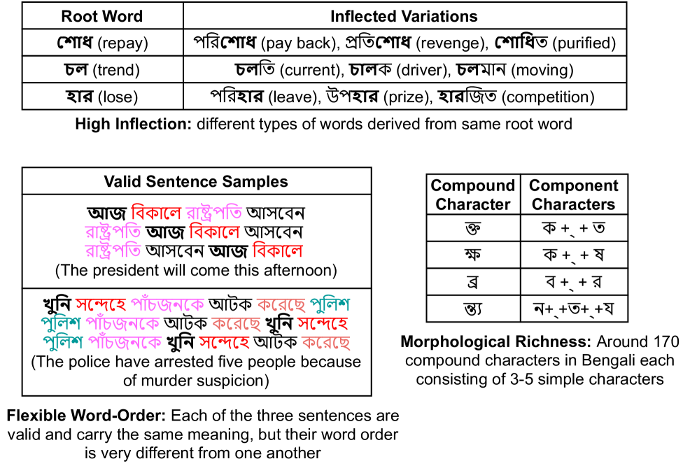
Figure 1: Bengali language unique characteristics

State-of-the-art (SOTA) techniques for LM can be categorized into three sub-domains of deep learning: (i) convolutional neural network (CNN) (Pham, Kruszewski, and Boleda 2016; Wang, Huang, and Deng 2018) (ii) recurrent neural network (Bojanowski et al. 2017; Mikolov et al. 2012; Kim et al. 2015; Gerz et al. 2018), and (iii) Transformer attention network (Al-Rfou et al. 2019; Vaswani et al. 2017; Irie et al. 2019; Ma et al. 2019). Long Short Term Memory (LSTM) based models, which are suitable for learning sequence and word order information, are not effective for modeling Bengali and Hindi due to their flexible word order characteristic. On the other hand, Transformers use dense layer based multi-head attention mechanism. They lack the ability to learn local patterns in sentence level, which in turn puts negative effect on modeling languages with loosely bound word order. Most importantly, neither LSTMs nor Transformers use any suitable measure to learn intra-word level local pattern necessary for modeling highly inflected and morphologically rich languages.

We observe that learning inter (flexible word order) and intra (high inflection and morphological richness) word local patterns is of paramount importance for Bengali and Hindi LM. To accommodate such characteristics, we design a novel CNN architecture, namely Coordinated CNN (CoCNN) that achieves SOTA performance with low training time. In particular, CoCNN consists of two learnable convolutional sub-models: word level (Vocabulary Learner (VL)) and sentence level (Terminal Coordinator (TC)). VL is designed for syllable pattern learning, whereas TC serves the purpose of word coordination learning while maintaining positional independence, which suits the flexible word order of Bengali and Hindi. CoCNN does not explicitly incorporate any self attention mechanism like Transformers; rather it relies on TC for emphasizing on important word patterns. CoCNN achieves significantly better performance than pretrained BERT for Bengali and Hindi LM with 16X less parameters. We further enhance CoCNN by introducing skip connection and parallel convolution branches in VL and TC, respectively. This modified architecture (with negligible increase in parameter number) is named as CoCNN+. We validate the effectiveness of CoCNN+ on a number of tasks that include next word prediction in erroneous setting, text classification, sentiment analysis and spell checking. CoCNN+ shows superior performance than contemporary LSTM based models and pretrained BERT.

In summary, the contributions of this paper are as follows:

• We propose an end to end trainable CNN architecture CoCNN based on the coordination of two CNN sub-models.

• We perform an in-depth analysis and comparison on different SOTA LMs in three paradigms: CNN, LSTM, and Transformer. With an extensive set of experiments, we show that CoCNN shows superior performance than LSTM and Transformer based models in spite of being memory efficient.

• We further show that simple modifications in CoCNN can give us even more superior performance in terms of Bengali and Hindi language modeling and other downstream tasks like text classification and sentiment analysis.

• We show the potential of VL sub-model of CoCNN+ as an effective spell checker for Bengali language.

2 Our Approach

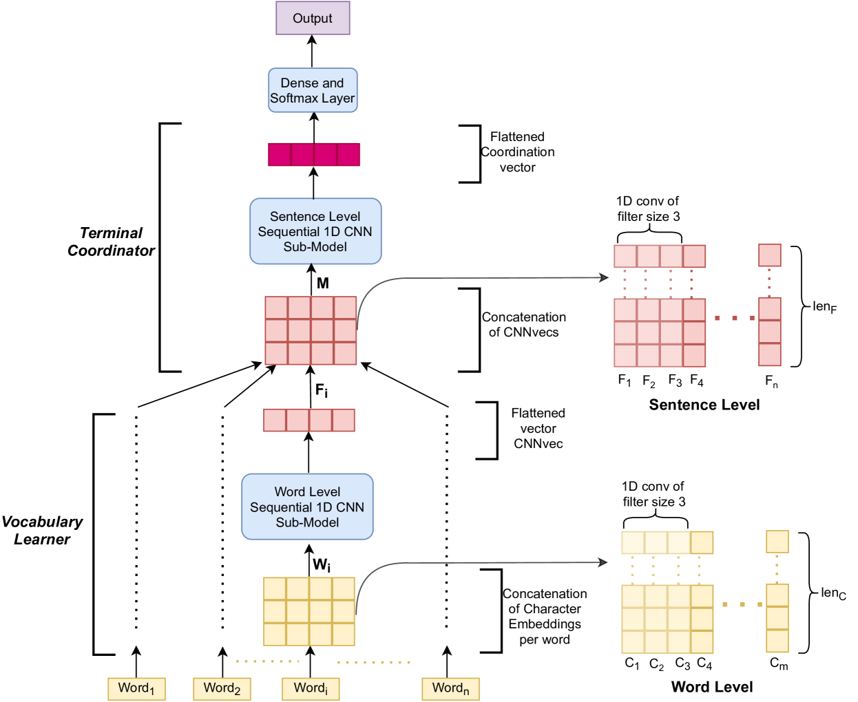
Figure 2: 1D CNN based CoCNN architecture

Traditional CNN based approaches (Pham, Kruszewski, and Boleda 2016) represent the entire input sentence/ paragraph using a matrix of size $S_{N}\times S_{V}$, where $S_{N}$ and $S_{V}$ represent number of characters in the sentence/ paragraph and the character representation vector size, respectively. In such character based approach, the model does not have the ability to consider each word in the sentence as a separate entity. However, it is important to understand the contextual meaning of each word and to find out relationship among those words for sentence semantics understanding. Our proposed Coordinated CNN (CoCNN) is aimed to achieve this feat. Figure 2 illustrates CoCNN that has two major components. Vocabulary Learner component works at word level, while Terminal Coordinator component works at sentence/ paragraph level. Both of these components are 1D CNN based sub-model at their core and are trained end-to-end.

2.1 Vocabulary Learner

Vocabulary Learner (VL) is used to transform each input word into a vector representation called CNNvec. We represent each input word $Word_{i}$ by a matrix $W_{i}$. $W_{i}$ consists of $m$ vectors each of size $len_{C}$. These vectors $\vec{C_{1}},\vec{C_{2}},\ldots\vec{C_{m}}$ represent one hot vector of character $C_{1},C_{2},\ldots C_{m}$, respectively of $Word_{i}$. Representation detail has been depicted in the bottom right corner of Figure 2. Applying 1D convolution (conv) layers on matrix $W_{i}$ helps in deriving key local patterns and sub-word information of $Word_{i}$. 1D conv operation starting from vector $\vec{C_{j}}$ of $W_{i}$ using a conv filter of size $K$ can be expressed as $1D\_Conv([\vec{C_{j}},\vec{C_{j+1}},\ldots\vec{C_{j+K-1}}],filter_{K})$ function. The output of this function is a scalar value. While using a stride of $s$, the next conv operation will start from vector $\vec{C_{j+s}}$ of $W_{i}$ and will provide us with another scalar value. Thus we get a vector as a result of applying one conv filter on matrix $W_{i}$. A conv layer has multiple such conv filters. After passing $W_{i}$ matrix through the first conv layer we obtain feature matrix $W^{1}_{i}$. Passing $W^{1}_{i}$ through the second conv layer provides us with feature matrix $W^{2}_{i}$. So, the $L^{th}$ conv layer provides us with feature matrix $W^{L}_{i}$. VL sub-model consists of such 1D conv layers standing sequentially one after the other. Conv layers near matrix $W_{i}$ are responsible for identifying key sub-word patterns of $Word_{i}$, while conv layers further away focus on different combinations of these key sub-word patterns. Such word level local pattern recognition plays key role in identifying semantic meaning of a word irrespective of inflection or presence of spelling error. Each intermediate conv layer output is batch normalized. The final conv layer output matrix $W^{L}_{i}$ is flattened and formed into a vector $F_{i}$ of size $len_{F}$. $F_{i}$ is the CNNvec representation of $Word_{i}$. We obtain CNNvec representation from each of our input words in a similar fashion applying the same CNN sub-model.

2.2 Terminal Coordinator

Terminal Coordinator (TC) takes the CNNvecs obtained from VL as input and returns a single Coordination vector as output which is used for final prediction. For $n$ words $Word_{1},Word_{2},\ldots Word_{n}$; we obtain $n$ such CNNvecs $\vec{F_{1}},\vec{F_{2}},\ldots\vec{F_{n}}$, respectively. Each CNNvec is of size $len_{F}$. Concatenating these CNNvecs provide us with matrix $M$ (details shown in the middle right portion of Figure 2). Applying 1D conv on matrix $M$ facilitates the derivation of key local patterns found in input sentence/ paragraph which is crucial for output prediction. 1D conv operation starting from $\vec{F_{i}}$ using a conv filter of size $K$ can be expressed as $1D\_Conv([\vec{F_{i}},\vec{F_{i+1}},\ldots\vec{F_{i+K-1}}],filter_{K})$ function. The output of this function is a scalar value. A sequential 1D CNN sub-model with design similar to VL (see Subsection 2.1) having different set of weights is employed on matrix $M$. Conv layers near $M$ are responsible for identifying key word clusters, while conv layers further away focus on different combinations of these key word clusters important for sentence or paragraph level local pattern recognition. The final output feature matrix obtained from the 1D CNN sub-model of TC is flattened to obtain the Coordination vector, a summary of important information obtained from the input word sequence in order to predict the correct output.

2.3 Attention to Patterns of Significance

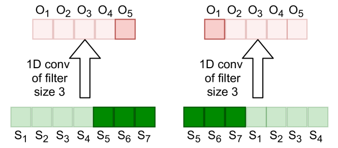
Figure 3: 1D convolution as a form of attention

There is no explicit attention mechanism in CoCNN unlike self attention based Transformers (Vaswani et al. 2017; Irie et al. 2019) or weighted attention based LSTMs (Bahdanau, Cho, and Bengio 2014; Luong, Pham, and Manning 2015). Attention mechanism is important for obtaining the importance of each input word in terms of output prediction. Figure 3 demonstrates an over simplified notion of how 1D conv implicitly imposes attention on a sequence containing 7 entities $S_{1},S_{2},\ldots S_{7}$. After employing a 1D conv filter of size 3 on this sequence representation, we obtain a vector containing values $O_{1},O_{2},\ldots O_{5}$, where we assume $O_{5}$ and $O_{1}$ to be the maximum for the left and the right figure, respectively. $O_{5}$ (left figure) is obtained by convolving input entity $S_{5}$, $S_{6}$ and $S_{7}$ situated at the end of input sequence. We can say that these three input entities have been paid more attention to by our conv filter than the other 4 entities. In the right figure, $S_{5}$, $S_{6}$ and $S_{7}$ are situated at the beginning of the input sequence. Our conv filter gives similar importance to this pattern irrespective of its position change. Such positional independence of important patterns helps in Bengali and Hindi LM where input words are loosely bound and words themselves are highly inflected. In CoCNN, such attention is imposed on characters of each word during CNNvec representation generation of that word using VL, while similar type of attention is imposed on words of our input sentence/ paragraph while obtaining Coordination vector using TC.

2.4 Extending CoCNN

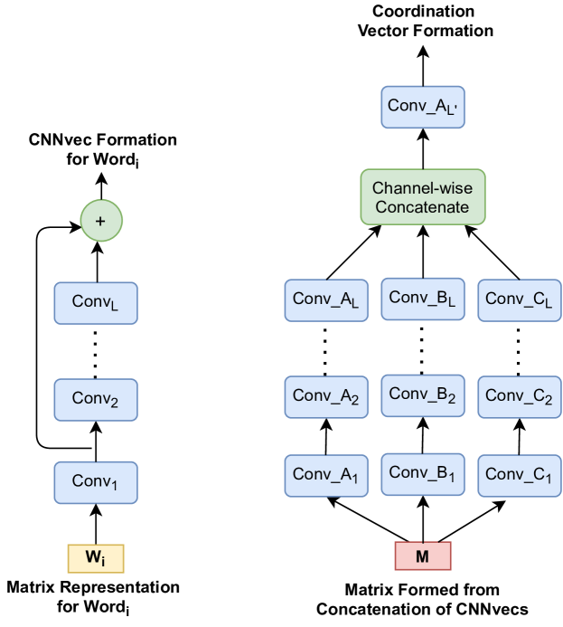
Figure 4: CoCNN+ architecture with its modified VL (left) and TC (right). $Conv_{L}$ means $L^{th}$ conv layer, whereas Conv_A means a conv layer with filter size A.

We perform two simple modifications in CoCNN to form CoCNN+ architecture with minimal increase in parameter number (see Figure 4).
First, we modify the CNN sub-model of VL. We add the output feature matrix of the first conv layer $Conv_{1}$ with the output feature matrix of the last conv layer $Conv_{L}$. We pass the resultant feature matrix on to subsequent layers (same as CoCNN) for CNNvec formation of $Word_{i}$. Such modification helps in two cases - (i) it eliminates the gradient vanishing problem of the first conv layer of VL and (ii) it gives CNNvec access to both low level and high level features of the corresponding input word.
Second, we modify the CNN sub-model of TC by passing matrix $M$ simultaneously to three 1D CNN branches. The conv filter sizes of the left, middle and right branches are $A$, $B$ and $C$, respectively; where, $A<B$ and $B<C$. The outputs from the three branches are concatenated channel-wise and are then passed on to the final conv layer having filter size $A$. The output feature matrix is passed on to subsequent layers (same as CoCNN) for Coordination vector formation. Multiple conv branches with different filter sizes help in learning both short and long range local patterns, especially when the input sentence or document is long.

3 Experimental Setup

3.1 Dataset Specifications

Bengali dataset consists of articles from online public news portals such as Prothom-Alo (Rahman 2017), BDNews24 (Khalidi 2015) and Nayadiganta (Mohiuddin 2019). The articles encompass domains such as politics, entertainment, lifestyle, sports, technology and literature. The Hindi dataset consists of Hindinews (Pandey 2018), Livehindustan (Shekhar 2018) and Patrika (Jain 2018) newspaper articles available open source in Kaggle encompassing similar domains. Nayadiganta (Bengali) and Patrika (Hindi) datasets have been used only as independent test sets. Detailed statistics of the datasets are provided in Table 1. Top words have been selected such that they cover at least 90% of the dataset. For each Bengali dataset, we have created a new version of the dataset by incorporating spelling errors using a probabilistic error generation algorithm (Sifat et al. 2020), which enables us to test the effectiveness of LMs for erroneous datasets.

Datasets	Unique Word No.	Unique Character No.	Top Word No.	Training Sample No.	Validation Sample No.
Prothom-Alo	260 K	75	13 K	5.9 M	740 K
BDNews24	170 K	72	14 K	2.9 M	330 K
Nayadiganta	44 K	73	_	_	280 K
Hindinews	37 K	74	5.5 K	87 K	10 K
Livehindustan	60 K	73	4.5 K	210 K	20 K
Patrika	28 K	73	_	_	307 K

Table 1: Dataset details (K and M denote $10^{3}$ and $10^{6}$ multiplier, respectively)

3.2 Performance Metric

We use perplexity (PPL) to assess the performance of the models for next word prediction task. Suppose, we have sample inputs $I_{1},I_{2},\dots,I_{n}$ and our model provides probability values $P_{1},P_{2},\ldots,P_{n}$, respectively for their ground truth output tokens. Then the PPL score of our model for these samples can be computed as:

$PPL=\exp(-\frac{1}{n}\sum_{i=1}^{n}\ln(P_{i}))$

PPL as a metric emphasizes on a model’s ability to understand a language instead of emphasizing on predicting the ground truth next word as output. For text classification and sentiment analysis, we use accuracy and F1 score as our performance metric.

3.3 Model Optimization

For model optimization, we use SGD optimizer with a learning rate of 0.001 while constraining the norm of the gradients to below 5 for exploding gradient problem elimination. We use Categorical Cross-Entropy loss for model weight update and dropout (Hinton et al. 2012) with probability 0.3 between the dense layers for regularization. We use Relu (Rectified Linear Unit) as hidden layer activation function. We use a batch size of 64. As we apply batch normalization on CNN intermediate outputs, we do not use any other regularization effect such as dropout on these layers (Luo et al. 2018).

We use Anaconda 3 with Python 3.8 version and Tensorflow 2.6.0 framework for our implementation. We use two GPU servers for training our models: (i) 12 GB Nvidia Titan Xp GPU, Intel(R) Core(TM) i7-7700 CPU (3.60GHz) processor model (ii) 32 GB RAM with 8 cores 24 GB Nvidia Tesla K80 GPU, Intel(R) Xeon(R) CPU (2.30GHz) processor model

3.4 CoCNN Hyperparameters

Our proposed CoCNN architecture has two main components. We specify the details of each of them in this subsection.

Vocabulary Learner Details

Vocabulary Learner sub-model consists of a character level embedding layer producing a 40 size vector from each character, then four consecutive layers each consisting of 1D convolution (batch normalization and Relu activation in between each pair of convolution layers) and finally, a 1D global maxpooling in order to obtain CNNvec representation from each input word. The four 1D convolution layers consist of $(32,2),(64,3),(64,3),(128,4)$ convolution, respectively. Here the first and second element of each tuple denote number of convolution filters and kernel size, respectively. As we can see, the filter size and number of filters of the convolution layers are monotonically increasing as architecture depth increases. It is because deep convolution layers need to learn the combination of various low level features which is a more difficult task compared to the task of shallow layers that include extraction of low level features.

Terminal Coordinator Details

The Terminal Coordinator sub-model used in CoCNN architecture uses six convolution layers which consist of $(32,2),(64,3),(64,3),(96,3),(128,4),(196,4)$ convolution. Its design is similar to that of Vocabulary Learner sub-model. The final output feature matrix obtained from this CNN sub-model is flattened to get the Coordination vector. After passing this vector through a couple of dense layers, we use Softmax activation function at the final output layer to get the predicted output.

3.5 CoCNN+ Hyperparameters

The CNN sub-model of Vocabulary Learner in CoCNN+ is the same as CoCNN except for one aspect (see Figure 4) - we change the first convolution layer to have 128 filters of size 2 instead of 32 filters. This is done to respect the matrix dimensionality during skip connection based addition.

Instead of providing a sequential 1D CNN sub-model in Terminal Coordinator, we provide three parallel branches each consisting of four convolution layers (see Figure 4) where the filter numbers are 32, 64, 96 and 128. The filter size of the leftmost, middle and the rightmost branch are 3, 5 and 7, respectively. All convolution operations are dimension preserving through the use of padding. The feature matrices of all three of these branches are concatenated channel-wise and finally, this concatenated matrix is passed on to a final convolution layer with 196 filters of size 3.

3.6 Hardware Specifications

We use Python 3.8 and Tensorflow 2.6.0 package for our implementation. We use three GPU servers for training our models. Their specifications are as follows:

• 12 GB Nvidia Titan Xp GPU, Intel(R) Core(TM) i7-7700 CPU (3.60GHz) processor model, 32 GB RAM with 8 cores

• 24 GB Nvidia Tesla K80 GPU, Intel(R) Xeon(R) CPU (2.30GHz) processor model, 12 GB RAM with 2 cores

• 8 GB Nvidia RTX 2070 GPU, Intel(R) Core(TM) CPU (2.20GHz) processor model, 32 GB RAM with 7 cores

4 Results and Discussion

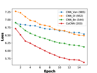
(a) CNN paradigm

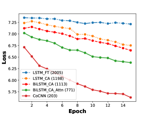
(b) LSTM paradigm

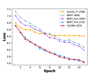
(c) Transformer paradigm

Figure 5: Comparing CoCNN with SOTA architectures from CNN, LSTM and Transformer paradigm on Prothom-Alo validation set. The score shown beside each model name denotes that model’s PPL score on Prothom-Alo validation set after 15 epochs of training. Note that this dataset contains synthetically generated spelling errors.

4.1 Comparing CoCNN with Other CNNs

We compare CoCNN with three other CNN-based baselines (see Figure 5a). CNN_Van is a simple sequential 1D CNN model of moderate depth (Pham, Kruszewski, and Boleda 2016). It considers the full input sentence/ paragraph as a matrix. The matrix consists of character representation vectors. CNN_Dl uses dilated conv in its CNN layers which allows the model to have a larger field of view (Roy 2019). Such change in conv strategy shows slight performance improvement. CNN_Bn has the same setting as of CNN_Van, but uses batch normalization on intermediate conv layer outputs. Such measure shows significant performance improvement in terms of loss and PPL score. Proposed CoCNN surpasses the performance of CNN_Bn by a wide margin. We believe that the ability of CoCNN to consider each word of a sentence as a separate meaningful entity is the reason behind this drastic improvement.

4.2 Comparing CoCNN with SOTA LSTMs

We compare CoCNN with four LSTM-based models (see Figure 5b). Two LSTM layers are stacked on top of each other in all four of these models. We do not compare with LSTM models that use Word2vec (Rong 2014) representation as this representation requires fixed size vocabulary. In spelling error prone setting, vocabulary size is theoretically infinite. We start with LSTM_FT, an architecture using sub-word based FastText representation (Athiwaratkun, Wilson, and Anandkumar 2018; Bojanowski et al. 2017). Character aware learnable layers per LSTM time stamp form the new generation of SOTA LSTMs (Mikolov et al. 2012; Kim et al. 2015; Gerz et al. 2018; Assylbekov et al. 2017). LSTM_CA acts as their representative by introducing variable size parallel conv filter output concatenation as word representation. The improvement over LSTM_FT in terms of PPL score is almost double. Instead of unidirectional many to one LSTM, we introduce bidirectional LSTM in LSTM_CA to form BiLSTM_CA which shows slight performance improvement. We introduce Bahdanu attention (Bahdanau, Cho, and Bengio 2014) on BiLSTM_CA to form BiLSTM_CA_Attn architecture. Such measure shows further performance boost. CoCNN shows almost four times improvement in PPL score compared to BiLSTM_CA_Attn. If we compare Figure 5b and 5a, we can see that CNNs perform relatively better than LSTMs in general for Bengali LM. LSTMs have a tendency of learning sequence order information which imposes positional dependency. Such characteristic is unsuitable for Bengali and Hindi with flexible word order.

4.3 Comparing CoCNN with SOTA Transformers

We compare CoCNN with four Transformer-based models (see Figure 5c). We use popular FastText word representation with all compared transformers. Our comparison starts with Vanilla_Tr, a single Transformer encoder (similar to the Transformer designed by Vaswani et al. (2017)). In BERT, we stack 12 transformers on top of each other where each Transformer encoder has more parameters than the Transformer of Vanilla_Tr (Devlin et al. 2018; Irie et al. 2019). BERT with its large depth and enhanced encoders almost double the performance shown by Vanilla_Tr. We do not pretrain this BERT architecture. We follow the Transformer architecture designed by Al-Rfou et al. (2019) and introduce auxiliary loss after the Transformer encoders situated near the bottom of the Transformer stack of BERT to form BERT_Aux. Introduction of such auxiliary losses show moderate improvement of performance. BERT_Pre is the pretrained version of BERT. We follow the word masking based pretraining scheme of Liu et al. (2019). The Bengali pretraining corpus consists of Prothom Alo (Rahman 2017) news articles dated from 2014-2017 and BDNews24 (Khalidi 2015) news articles dated from 2015-2017. The performance of BERT jumps up more than double when such pretraining is applied. CoCNN without utilizing any pretraining achieves marginally better performance than BERT_Pre. Unlike Transformer encoders, conv imposes attention with a view to extracting important patterns from the input to provide the correct output (see Subsection 2.3). Furthermore, VL of CoCNN is suitable for deriving semantic meaning of each input word in highly inflected and error prone settings.

4.4 Comparing BERT_Pre, CoCNN and CoCNN+

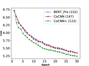
(a) Plot on Bengali dataset

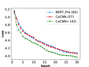
(b) Plot on Hindi dataset

Figure 6: Comparing BERT_Pre, CoCNN and CoCNN+ on Bengali (Prothom-Alo) and Hindi (Hindinews and Livehindustan merged) validation set. The score shown beside each model name denotes that model’s PPL score after 30 epochs of training on corresponding training set.

Datasets	Error?	BERT_ Pre	Co- CNN	Co- CNN+
Prothom-Alo	Yes	152	147	122
	No	117	114	99
BDNews24	Yes	201	193	170
	No	147	141	123
Hindinews + Livehindustan	No	65	57	42
Nayadiganta	Yes	169	162	143
	No	136	133	118
Patrika	No	67	57	44

Table 2: Comparing (PPL) BERT_Pre, CoCNN and CoCNN+

BERT_Pre is the only model showing performance close to CoCNN in terms of validation loss and PPL score (see Figure 5). We compare these two models with CoCNN+. we train the models for 30 epochs on several Bengali and Hindi datasets and obtain their PPL scores on corresponding validation sets (training and validation set were split at 80%-20% ratio). Bengali datasets include Prothom-Alo, BDNews24; while Hindi dataset includes Hindinews, Livehindustan. We use Nayadiganta and Patrika dataset for Bengali and Hindi independent test set, respectively. The Hindi pretraining corpus consists of Hindi Oscar Corpus (Thakur 2019), preprocessed Wikipedia articles (Gaurav 2019), HindiEnCorp05 dataset (Bojar et al. 2014) and WMT Hindi News Crawl data (Barrault et al. 2019). From the graphs of Figure 6 and PPL score comparison Table 2, it is evident that CoCNN marginally outperforms its nemesis BERT_Pre in all cases, while CoCNN+ outperforms both CoCNN and BERT_Pre by a significant margin. There are 8 sets of PPL scores in Table 2 for the three models on eight different dataset settings. We use these scores to perform one tailed paired t-test in order to determine whether the reduction of PPL score seen in CoCNN compared to BERT_Pre is statistically significant when P-value threshold is set to 0.05. The statistical test shows that the improvement is significant. Similarly, CoCNN+ significantly outperforms CoCNN in terms of achieved PPL scores. Number of parameters of BERT_Pre, CoCNN and CoCNN+ are 74 M, 4.5 M and 4.8 M, respectively. Though the parameter number of CoCNN+ and CoCNN is close, CoCNN+ has 15X fewer parameters than BERT_Pre.

4.5 Comparison in Downstream Tasks

We first show the performance comparison of CoCNN+ with BERT_Pre in three downstream tasks. Then we present the performance of one of our key components VL for spell checking task.

Dataset	Metric	BERT_Pre	CoCNN+
Question Classify	Acc	91.3%	93.7%
	F1	0.905	0.926
Product Review	Acc	84.4%	86.2%
	F1	0.841	0.86
Hate Speech	Acc	78%	79.2%
	F1	0.77	0.781

Table 3: Performance comparison between BERT_Pre and CoCNN+ in three downstream tasks

Comparison in Downstream Tasks.

We have compared BERT_Pre and CoCNN+ in three different downstream tasks:
(1) Bengali Question Classification (QC): This task consists of six classes (entity, numeric, human, location, description and abbreviation type question). The dataset has 3350 question samples (Islam et al. 2016).
(2) Hindi Product Review Classification: The task is to classify a review into positive or negative class where the dataset consists of 2355 sample reviews (Kakwani 2020).
(3) Hindi Hate Speech Detection: The task is to identify whether a provided speech is a hate speech or not. The dataset consists of 3654 speeches (HASOC 2019).

We use five fold cross validation while performing comparison on these datasets (see mean results in Table 3) in terms of accuracy and F1 score). One tailed independent t-test with a P-value threshold of 0.05 have been performed on the 5 validation F1 scores obtained from five fold cross validation of each of the two models. Our statistical test results validate the significance of the improvement shown by CoCNN+ for all three of the mentioned tasks.

Vocabulary Learner as Spell Checker.

Spell Checker Algorithm	Synthetic Error	Real Error
Vocabulary Learner	71.1%	61.1%
Phonetic Rule	61.5%	32.5%
Clustering Rule	51.8%	43.8%

Table 4: Bengali spelling correction (accuracy)

We also investigate the potential of VL of CoCNN+ as a Bengali spell checker (SC). Both CoCNN and CoCNN+ model use VL for producing CNNvec representation from each input word. We extract the CNN sub-model of VL from our trained (on Prothom-Alo dataset) CoCNN+ model. We produce CNNvec for all 13 K top words of Prothom-Alo dataset. For any error word, $W_{e}$, we can generate its CNNvec $V_{e}$ using VL. We can calculate cosine similarity, $Cos_{i}$ between $V_{e}$ and CNNvec $V_{i}$ of each top word $W_{i}$. Higher cosine similarity means greater probability of being the correct version of $W_{e}$. We have discovered such approach to be effective for correct word generation. Recently, a phonetic rule based approach has been proposed by Saha et al. (2019), where a hybrid of Soundex (UzZaman and Khan 2004) and Metaphone (UzZaman and Khan 2005) algorithm has been used for Bengali word level SC. Another SC proposed in recent time has taken a clustering based approach (Mandal and Hossain 2017). We compare our proposed VL based SC with these two existing SCs (see Table 4). Both the real and synthetic error dataset consist of 20k error words formed from the top 13k words of Prothom-Alo dataset. The real error dataset has been collected from a wide range of Bengali native speakers using an easy to use web app. Results show the superiority of our proposed SC over existing approaches.

5 Related Works

Although a significant number of works for LM of high resource languages like English and Chinese are available, very few researches of significance for LM in low resource languages like Bengali and Hindi exist. In this section, we mainly summarize major LM related research works.

Sequence order information based statistical RNN models such as LSTM and GRU have been popular for LM tasks (Mikolov et al. 2011). Sundermeyer, Schlüter, and Ney (2012) showed the effectiveness of LSTM for English and French LM. The regularizing effect on LSTM was investigated by Merity, Keskar, and Socher (2017). SOTA LSTM models learn sub-word information in each time stamp. Bojanowski et al. (2017) proposed a morphological information oriented character N-gram based word vector representation. It was improved by Athiwaratkun, Wilson, and Anandkumar (2018) and is known as FastText. Mikolov et al. (2012) proposed a technique for learning sub-word level information from data, while such idea was integrated in a character aware LSTM model by Kim et al. (2015). Takase, Suzuki, and Nagata (2019) further improved word representation by combining ordinary word level and character-aware embedding. Assylbekov et al. (2017) has shown that character-aware neural LMs outperform syllable-aware ones. Gerz et al. (2018) evaluated such models on 50 morphologically rich languages.

Self attention based Transformers have become the SOTA mechanism for sequence to sequence modeling in recent years (Vaswani et al. 2017). Some recent works have explored the use of such models in LM. Deep Transformer encoders outperform stacked LSTM models (Irie et al. 2019). A deep stacked Transformer model utilizing auxiliary loss was proposed by Al-Rfou et al. (2019) for character level language modeling. The multi-head self attention mechanism was replaced by a multi-linear attention mechanism with a view to improving LM performance and reducing parameter number (Ma et al. 2019). Bengali and Hindi language, having unique characteristics, remain open as to what strategy to use for model development in such domains.

One dimensional version of CNNs have been used recently for text classification oriented tasks (Wang, Huang, and Deng 2018; Moriya and Shibata 2018; Le, Cerisara, and Denis 2018). Pham, Kruszewski, and Boleda (2016) studied CNN application in LM showing the ability of CNNs to extract LM features at a high level of abstraction. Furthermore, dilated conv was employed in Bengali LM with a view to solving long range dependency problem (Roy 2019).

6 Conclusion

We have proposed a CNN based architecture Coordinated CNN (CoCNN) that introduces two 1D CNN based key concepts: word level VL and sentence level TC. Detailed investigation in three deep learning paradigms: CNN, LSTM and Transformer, shows the effectiveness of CoCNN in Bengali and Hindi LM. We have also shown a simple but effective enhancement of CoCNN by introducing skip connection and parallel conv branches in the VL and TC portion, respectively. Future research may incorporate interesting ideas from existing SOTA 2D CNNs in CoCNN. Over-parametrization and innovative scheme for CoCNN pretraining are expected to increase its LM performance even further.

7 Acknowledgements

This work was supported by Bangladesh Information and Communication Technology (ICT) division [grant number: 56.00.0000.028.33.095.19- 85] as part of Enhancement of Bengali Language project.

References

- Al-Rfou et al. (2019) Al-Rfou, R.; Choe, D.; Constant, N.; Guo, M.; and Jones, L. 2019. Character-level language modeling with deeper self-attention. In Proceedings of the AAAI Conference on Artificial Intelligence, volume 33, 3159–3166.
- Assylbekov et al. (2017) Assylbekov, Z.; Takhanov, R.; Myrzakhmetov, B.; and Washington, J. N. 2017. Syllable-aware neural language models: A failure to beat character-aware ones. arXiv preprint arXiv:1707.06480.
- Athiwaratkun, Wilson, and Anandkumar (2018) Athiwaratkun, B.; Wilson, A. G.; and Anandkumar, A. 2018. Probabilistic fasttext for multi-sense word embeddings. arXiv preprint arXiv:1806.02901.
- Bahdanau, Cho, and Bengio (2014) Bahdanau, D.; Cho, K.; and Bengio, Y. 2014. Neural machine translation by jointly learning to align and translate. arXiv preprint arXiv:1409.0473.
- Barrault et al. (2019) Barrault, L.; Bojar, O.; Costa-jussà, M. R.; Federmann, C.; Fishel, M.; Graham, Y.; Haddow, B.; Huck, M.; Koehn, P.; Malmasi, S.; Monz, C.; Müller, M.; Pal, S.; Post, M.; and Zampieri, M. 2019. Findings of the 2019 Conference on Machine Translation (WMT19). In Proceedings of the Fourth Conference on Machine Translation (Volume 2: Shared Task Papers, Day 1), 1–61. Florence, Italy: Association for Computational Linguistics.
- Bojanowski et al. (2017) Bojanowski, P.; Grave, E.; Joulin, A.; and Mikolov, T. 2017. Enriching Word Vectors with Subword Information. Transactions of the Association for Computational Linguistics, 5: 135–146.
- Bojar et al. (2014) Bojar, O.; Diatka, V.; Straňák, P.; Tamchyna, A.; and Zeman, D. 2014. HindEnCorp 0.5. LINDAT/CLARIAH-CZ digital library at the Institute of Formal and Applied Linguistics (ÚFAL), Faculty of Mathematics and Physics, Charles University.
- Cai and Zhao (2016) Cai, D.; and Zhao, H. 2016. Neural word segmentation learning for Chinese. arXiv preprint arXiv:1606.04300.
- Devlin et al. (2018) Devlin, J.; Chang, M.-W.; Lee, K.; and Toutanova, K. 2018. Bert: Pre-training of deep bidirectional transformers for language understanding. arXiv preprint arXiv:1810.04805.
- Gao et al. (2002) Gao, J.; Goodman, J.; Li, M.; and Lee, K.-F. 2002. Toward a unified approach to statistical language modeling for Chinese. ACM Transactions on Asian Language Information Processing (TALIP), 1(1): 3–33.
- Gaurav (2019) Gaurav. 2019. Wikipedia. https://www.kaggle.com/disisbig/hindi-wikipedia-articles-172k.
- Gerz et al. (2018) Gerz, D.; Vulić, I.; Ponti, E.; Naradowsky, J.; Reichart, R.; and Korhonen, A. 2018. Language Modeling for Morphologically Rich Languages: Character-Aware Modeling for Word-Level Prediction. Transactions of the Association for Computational Linguistics, 6: 451–465.
- HASOC (2019) HASOC. 2019. Hindi Hate speech dataset. https://hasocfire.github.io/hasoc/2019/dataset.html.
- Hinton et al. (2012) Hinton, G. E.; Srivastava, N.; Krizhevsky, A.; Sutskever, I.; and Salakhutdinov, R. R. 2012. Improving neural networks by preventing co-adaptation of feature detectors. arXiv preprint arXiv:1207.0580.
- Irie et al. (2019) Irie, K.; Zeyer, A.; Schlüter, R.; and Ney, H. 2019. Language modeling with deep Transformers. arXiv preprint arXiv:1905.04226.
- Islam et al. (2016) Islam, M. A.; Kabir, M. F.; Abdullah-Al-Mamun, K.; and Huda, M. N. 2016. Word/phrase based answer type classification for bengali question answering system. In 2016 5th International Conference on Informatics, Electronics and Vision (ICIEV), 445–448. IEEE.
- Jain (2018) Jain, B. 2018. Patrika. https://epaper.patrika.com/.
- Kakwani (2020) Kakwani, D. 2020. AI4Bharat. https://github.com/ai4bharat.
- Khalidi (2015) Khalidi, T. I. 2015. BDnews24. https://bdnews24.com/.
- Kim et al. (2015) Kim, Y.; Jernite, Y.; Sontag, D.; and Rush, A. M. 2015. Character-aware neural language models. arXiv preprint arXiv:1508.06615.
- Le, Cerisara, and Denis (2018) Le, H. T.; Cerisara, C.; and Denis, A. 2018. Do convolutional networks need to be deep for text classification? In Workshops at the Thirty-Second AAAI Conference on Artificial Intelligence.
- Liu et al. (2019) Liu, Y.; Ott, M.; Goyal, N.; Du, J.; Joshi, M.; Chen, D.; Levy, O.; Lewis, M.; Zettlemoyer, L.; and Stoyanov, V. 2019. Roberta: A robustly optimized bert pretraining approach. arXiv preprint arXiv:1907.11692.
- Luo et al. (2018) Luo, P.; Wang, X.; Shao, W.; and Peng, Z. 2018. Towards understanding regularization in batch normalization. arXiv preprint arXiv:1809.00846.
- Luong, Pham, and Manning (2015) Luong, M.-T.; Pham, H.; and Manning, C. D. 2015. Effective approaches to attention-based neural machine translation. arXiv preprint arXiv:1508.04025.
- Ma et al. (2019) Ma, X.; Zhang, P.; Zhang, S.; Duan, N.; Hou, Y.; Zhou, M.; and Song, D. 2019. A tensorized transformer for language modeling. In Advances in Neural Information Processing Systems, 2232–2242.
- Mandal and Hossain (2017) Mandal, P.; and Hossain, B. M. 2017. Clustering-based Bangla spell checker. In 2017 IEEE International Conference on Imaging, Vision & Pattern Recognition (icIVPR), 1–6. IEEE.
- Merity, Keskar, and Socher (2017) Merity, S.; Keskar, N. S.; and Socher, R. 2017. Regularizing and optimizing LSTM language models. arXiv preprint arXiv:1708.02182.
- Mikolov et al. (2011) Mikolov, T.; Kombrink, S.; Burget, L.; Černockỳ, J.; and Khudanpur, S. 2011. Extensions of recurrent neural network language model. In 2011 IEEE international conference on acoustics, speech and signal processing (ICASSP), 5528–5531. IEEE.
- Mikolov et al. (2012) Mikolov, T.; Sutskever, I.; Deoras, A.; Le, H.-S.; Kombrink, S.; and Cernocky, J. 2012. Subword language modeling with neural networks. preprint (http://www. fit. vutbr. cz/imikolov/rnnlm/char. pdf), 8: 67.
- Mohiuddin (2019) Mohiuddin, A. 2019. Nayadiganta. https://www.dailynayadiganta.com/.
- Moriya and Shibata (2018) Moriya, S.; and Shibata, C. 2018. Transfer learning method for very deep CNN for text classification and methods for its evaluation. In 2018 IEEE 42nd Annual Computer Software and Applications Conference (COMPSAC), volume 2, 153–158. IEEE.
- Pandey (2018) Pandey, S. 2018. Hindinews. https://www.dailyhindinews.com/.
- Pham, Kruszewski, and Boleda (2016) Pham, N.-Q.; Kruszewski, G.; and Boleda, G. 2016. Convolutional neural network language models. In Proceedings of the 2016 Conference on Empirical Methods in Natural Language Processing, 1153–1162.
- Rahman (2017) Rahman, M. 2017. Prothom-Alo. https://www.prothomalo.com/.
- Rong (2014) Rong, X. 2014. word2vec parameter learning explained. arXiv preprint arXiv:1411.2738.
- Roy (2019) Roy, S. 2019. Improved Bangla Language Modeling with Convolution. In 2019 1st International Conference on Advances in Science, Engineering and Robotics Technology (ICASERT), 1–4. IEEE.
- Saha et al. (2019) Saha, S.; Tabassum, F.; Saha, K.; and Akter, M. 2019. BANGLA SPELL CHECKER AND SUGGESTION GENERATOR. Ph.D. thesis, United International University.
- Shekhar (2018) Shekhar, S. 2018. Livehindustan. https://www.livehindustan.com/.
- Sifat et al. (2020) Sifat, M.; Rahman, H.; Rahman, C. R.; Rafsan, M.; Rahman, M.; et al. 2020. Synthetic Error Dataset Generation Mimicking Bengali Writing Pattern. arXiv preprint arXiv:2003.03484.
- Staal (1963) Staal, J. F. 1963. Sanskrit and sanskritization. The Journal of Asian Studies, 22(3): 261–275.
- Sundermeyer, Schlüter, and Ney (2012) Sundermeyer, M.; Schlüter, R.; and Ney, H. 2012. LSTM neural networks for language modeling. In Thirteenth annual conference of the international speech communication association.
- Takase, Suzuki, and Nagata (2019) Takase, S.; Suzuki, J.; and Nagata, M. 2019. Character n-gram embeddings to improve RNN language models. In Proceedings of the AAAI Conference on Artificial Intelligence, volume 33, 5074–5082.
- Thakur (2019) Thakur, A. 2019. Hindi OSCAR Corpus. https://www.kaggle.com/abhishek/hindi-oscar-corpus.
- UzZaman and Khan (2004) UzZaman, N.; and Khan, M. 2004. A bangla phonetic encoding for better spelling suggesions. Technical report, BRAC University.
- UzZaman and Khan (2005) UzZaman, N.; and Khan, M. 2005. A double metaphone encoding for bangla and its application in spelling checker. In 2005 International Conference on Natural Language Processing and Knowledge Engineering, 705–710. IEEE.
- Vaswani et al. (2017) Vaswani, A.; Shazeer, N.; Parmar, N.; Uszkoreit, J.; Jones, L.; Gomez, A. N.; Kaiser, Ł.; and Polosukhin, I. 2017. Attention is all you need. In Advances in neural information processing systems, 5998–6008.
- Wang, Huang, and Deng (2018) Wang, S.; Huang, M.; and Deng, Z. 2018. Densely Connected CNN with Multi-scale Feature Attention for Text Classification. In IJCAI, 4468–4474.
- Yang, Tseng, and Chen (2016) Yang, T.-H.; Tseng, T.-H.; and Chen, C.-P. 2016. Recurrent neural network-based language models with variation in net topology, language, and granularity. In 2016 International Conference on Asian Language Processing (IALP), 71–74. IEEE.