Benchmarking Quantum Simulators

Abstract

Time-Averaged Mixed-state Equivalence (TAME) is used to benchmark quantum simulators with classical computing resources. The classical computation is feasible even if direct computation of the real-time dynamics is prohibitively costly.

I Time-Averaged Mixed-state Equivalence

Time-Averaged Mixed-state Equivalence (TAME) relates the real-time dynamics of pure quantum states and the expectation values of mixed quantum states.

I.1 Time-Averaged Dynamics

An observable $\hat{O}$ undergoes time evolution governed by a Hamiltonian $\hat{H}$:

$$\hat{H} =\sum_{\alpha}\mathcal{E}_{\alpha}\ket{\alpha}\kern-1.49994pt\bra{\alpha},$$ (I.1)

$$\hat{O} =\sum_{\alpha,\beta}\mathcal{O}_{\alpha,\beta}\ket{\alpha}\kern-1.49994pt\bra{\beta}$$ (I.2)

The real-time dynamics of $\hat{O}$ are as follows [1]:

$${{\hat{O}(t)=\kern 1.66672pt\text{{\hbox{e^{\scalebox{0.92}{}}}}}}\kern 1.66672pt\hat{O}\kern 1.66672pt\text{{\hbox{e^{-\scalebox{0.92}{}}}}}}$$ (I.3)

$${{{\hat{O}(t)=\sum_{\alpha,\beta}\text{{\hbox{\mathcal{O}_{\scalebox{0.78}{}}}}}}\kern 1.66672pt\text{{\hbox{\scalebox{1.05}{}}^{-\scalebox{0.92}{}}}}}}\ket{\alpha}\kern-1.49994pt\bra{\beta}$$ (I.4)

The time-averaged observable is the following:

$$\hat{\Omega}=\lim_{t\rightarrow\infty}\frac{1}{t}\int_{0}^{t}\kern 1.66672ptdt^{{}^{\prime}}\kern 1.66672pt\hat{O}(t^{{}^{\prime}})$$ (I.5)

$$\hat{\Omega}=\sum_{\alpha}\mathcal{O}_{\alpha,\alpha}\ket{\alpha}\kern-1.49994pt\bra{\alpha}$$ (I.6)

The time-averaged expectation value of a pure state $\ket{\psi}$ is the following:

$$\braket{\psi}{\kern 1.00006pt\hat{\Omega}\kern 1.00006pt}{\psi}=\sum_{\alpha}|c_{\alpha}|^{2}\kern 1.66672pt\mathcal{O}_{\alpha,\alpha}$$ (I.7)

$$\ket{\psi}=\sum_{\alpha}c_{\alpha}\ket{\alpha}$$ (I.8)

I.2 Mixed State Expectation Values

A mixed quantum state is composed of an ensemble of pure states $\ket{\text{$\psi_{k}$}}$, with observational probabilities $p_{k}$. Its density matrix [2, 3] is the following:

$$\rho =\sum_{k}\text{$p_{k}$}\Ket{\text{$\psi_{k}$}}\kern-1.49994pt\bra{\text{$\psi_{k}$}},$$ (I.9)

$$=\sum_{\alpha,\beta}\mathcal{P}_{\alpha,\beta}\ket{\alpha}\kern-1.49994pt\bra{\beta}$$ (I.10)

The expectation value of $\hat{O}$ is as follows:

$$\braket{\hat{O}}=\text{Tr}\Big{[}\rho\kern 1.66672pt\hat{O}\kern 1.00006pt\Big{]}$$ (I.11)

$$\braket{\hat{O}}=\sum_{\alpha,\beta}\mathcal{P}_{\alpha,\beta}\kern 1.66672pt\mathcal{O}_{\beta,\alpha}$$ (I.12)

Orthodox mixed states commute with the Hamiltonian:

$$\ \ \ \ \Big{[}\kern 1.00006pt\tilde{\rho},\hat{H}\kern 1.00006pt\Big{]}=0$$ (I.13)

$$\tilde{\rho}=\sum_{\alpha}\tilde{\mathcal{P}}_{\alpha}\ket{\alpha}\kern-1.49994pt\bra{\alpha}$$ (I.14)

The orthodox expectation value is the following:

$$\text{Tr}\Big{[}\tilde{\rho}\kern 1.66672pt\hat{O}\kern 1.00006pt\Big{]}=\sum_{\alpha}\tilde{\mathcal{P}}_{\alpha}\kern 1.66672pt\mathcal{O}_{\alpha,\alpha}$$ (I.15)

Density matrices must be positive semi-definite with $\text{Tr}(\rho)=1$ [4], which requires the following conditions to be satisfied:

$$\sum_{\alpha}\tilde{\mathcal{P}}_{\alpha}=1,\ \ \tilde{\mathcal{P}}_{\alpha}\in\mathbbm{R}^{+}$$ (I.16)

The time-averaged expectation values of each pure state are equivalent to the expectation values of an orthodox mixed state. This mapping is not one-to-one, as a continuum of pure states share a corresponding orthodox mixed state (Figure 1).

I.3 Coarse-Grained TAME

TAME is coarse-grained by integrating over the pure states and the orthodox mixed states [5, 6, 7, 8].

The coarse-grained time-averaged expectation value is obtained by integrating over all pure states:

$$\braket{\hat{\Omega}}_{c} =\int d\psi\ \braket{\psi}{\kern 1.00006pt\hat{\Omega}\kern 1.00006pt}{\psi}$$ (I.17)

$$=\int d\psi\ \sum_{\alpha}{|c_{\alpha}(\psi)|}^{2}\kern 1.66672pt\mathcal{O}_{\alpha,\alpha}$$ (I.18)

$$=\sum_{\alpha}\kern 1.66672pt\mathcal{O}_{\alpha,\alpha}\int d\psi\ \kern 1.66672pt{|c_{\alpha}(\psi)|}^{2}$$ (I.19)

$$=\text{Tr}\big{[}\hat{O}\big{]}\cdot\frac{1}{\text{dim}\{\hat{H}\}}$$ (I.20)

The coarse-grained orthodox expectation value is obtained by integrating over all orthodox mixed states:

$$\braket{\hat{O}}_{c} =\int d\tilde{\rho}\ \kern 1.00006pt\text{Tr}\Big{[}\tilde{\rho}\kern 1.66672pt\hat{O}\Big{]}$$

$$=\int d\tilde{\rho}\ \sum_{\alpha}\tilde{\mathcal{P}}_{\alpha}\kern 1.66672pt\mathcal{O}_{\alpha,\alpha}$$ (I.21)

$$=\sum_{\alpha}\mathcal{O}_{\alpha,\alpha}\int d\tilde{\rho}\ \tilde{\mathcal{P}}_{\alpha}$$ (I.22)

$$=\text{Tr}\big{[}\hat{O}\big{]}\cdot\frac{1}{\text{dim}\{\hat{H}\}}$$ (I.23)

Integrating over the pure states and the orthodox mixed states yields an identical quantity.

II Quantum Simulation Benchmark

Benchmarking the output of a quantum simulator [9, 10] can be accomplished with TAME. This requires determining the expectation values of orthodox mixed states using classical computing resources [11].

II.1 Orthodox Mixed State Computation

Orthodox mixed states can be expressed by applying positive-real functions $f(x)$ to the Hamiltonian:

$$\tilde{\rho}(f) =\frac{f(\hat{H})}{\text{Tr}\Big{[}f(\hat{H})\Big{]}}$$ (II.1)

$$=\frac{1}{\mathcal{Z}}\kern 1.66672ptf(\hat{H})$$ (II.2)

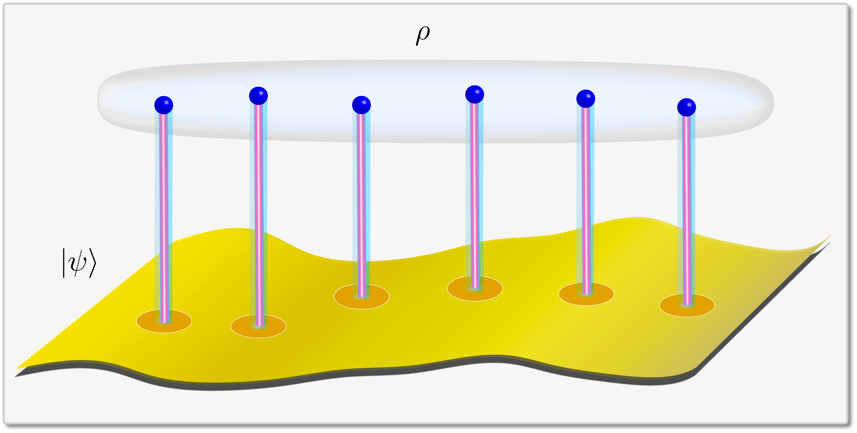
FIG. 1: [Upper Panel]: Orthodox mixed states (blue) reside in the space of mixed states (gray). [Lower Panel]: TAME relates each orthodox mixed state to a subset of states (golden) in the space of pure states (yellow).

A positive-real function can be expressed as follows:

$$f(x) =\int_{-\infty}^{\infty}dt\ \delta(x-t)\ f(t)$$ (II.3)

$$=\lim_{\sigma\rightarrow 0}\kern 1.66672pt\frac{1}{|\sigma|\sqrt{\pi}}\int_{-\infty}^{\infty}dt\ e^{-\Big{(}\scalebox{1.2}{$\frac{x-t}{\sigma}$}\Big{)}^{2}}\kern 1.66672ptf(t)$$ (II.4)

A general orthodox mixed state can be expressed as follows:

$$\tilde{\rho}(f)=\frac{1}{\mathcal{Z}}\Bigg{[}\lim_{\sigma\rightarrow 0}\kern 1.66672pt\frac{1}{|\sigma|\sqrt{\pi}}\int_{-\infty}^{\infty}dt\ e^{-\Big{(}\scalebox{1.2}{{\hbox{\frac{\hat{H}-t}{\sigma}}}}\Big{)}^{2}}\kern 1.66672ptf(t)\Bigg{]}$$ (II.5)

As such, it is sufficient to consider gaussian orthodox mixed states:

$$\tilde{\rho}_{g}(\epsilon,\sigma)=\frac{1}{\mathcal{Z}}\ e^{-\Big{(}\scalebox{1.2}{{\hbox{\frac{\hat{H}-\epsilon}{\sigma}}}}\Big{)}^{2}}$$ (II.6)

These can be re-expressed in terms of a Hermitian operator $\hat{K}$ and a real parameter $\tau$:

$${\tilde{\rho}_{g}(\epsilon,\sigma)=\frac{1}{\mathcal{Z}}\ \text{{\hbox{e^{-\scalebox{0.92}{}}}}}}$$ (II.7)

The expectation value of $\hat{O}$ is as follows:

$$\braket{\hat{O}} =\frac{1}{\mathcal{Z}}\text{Tr}\Big{[}\text{$e^{-\scalebox{0.92}{$\hat{K}\tau$}}$}\hat{O}\kern 1.00006pt\Big{]}$$ (II.8)

$$=\frac{1}{\mathcal{Z}}\sum_{a}\braket{a}{\kern 1.66672pt\text{$e^{-\scalebox{0.92}{$\hat{K}\tau$}}$}\kern 1.00006pt\hat{O}\kern 1.66672pt}{a}$$ (II.9)

The expectation value can be classically computed in a manner similar to the path integral [12]. This is accomplished by discretizing $e^{-\scalebox{0.92}{$\hat{K}\tau$}}$:

$${{{{\text{{\hbox{e^{-\scalebox{0.92}{}}}}}}\rightarrow\text{{\hbox{e^{-\scalebox{0.85}{}}}}}}\kern 1.00006pt\text{{\hbox{e^{-\scalebox{0.85}{}}}}}}\kern 1.00006pt\ldots\kern 1.00006pt\text{{\hbox{e^{-\scalebox{0.85}{}}}}}}$$ (II.10)

The identity is inserted between the matrix exponentials:

$$\begin{split}\text{$e^{-\scalebox{0.92}{$\hat{K}\tau$}}$}=&\sum_{a_{1}}\ldots\sum_{a_{N}}\ \ket{a_{1}}\kern-1.49994pt\bra{a_{1}}\text{$e^{-\scalebox{0.85}{$\hat{K}\Delta$}}$}\ket{a_{2}}\kern-1.49994pt\bra{a_{2}}\text{$e^{-\scalebox{0.85}{$\hat{K}\Delta$}}$}\ket{a_{3}}\kern-1.49994pt\bra{a_{3}}\\ &\qquad\ldots\ket{a_{N-1}}\kern-1.49994pt\bra{a_{N-1}}\text{$e^{-\scalebox{0.85}{$\hat{K}\Delta$}}$}\ket{a_{N}}\kern-1.49994pt\bra{a_{N}}\end{split}$$ (II.11)

This can be re-expressed as a sum over configurations $\vec{a}=\{a_{1},\cdots,a_{N}\}$:

$$e^{-\scalebox{0.92}{$\hat{K}\tau$}} =\sum_{\vec{a}}S(\vec{a})\ket{a_{1}}\kern-1.49994pt\bra{a_{N}}$$ (II.12)

$$S(\vec{a})=\bra{a_{1}} \text{$e^{-\scalebox{0.85}{$\hat{K}\Delta$}}$}\ket{a_{2}}\ldots\bra{a_{N-1}}\text{$e^{-\scalebox{0.85}{$\hat{K}\Delta$}}$}\ket{a_{N}}$$ (II.13)

The expectation value of $\hat{O}$ is the following:

$$\braket{\hat{O}} =\frac{1}{\mathcal{Z}}\sum_{a}\Bigg{[}\sum_{\vec{a}}\bra{a}S(\vec{a})\ket{a_{1}}\kern-1.49994pt\bra{a_{N}}\hat{O}\ket{a}\Bigg{]}$$ (II.14)

$$=\frac{1}{\mathcal{Z}}\sum_{\vec{a}}S(\vec{a})\bra{a_{N}}\hat{O}\ket{a_{1}}$$ (II.15)

$$=\frac{1}{\mathcal{Z}}\sum_{\vec{a}}\big{|}S(\vec{a})\big{|}\kern 1.66672ptO(\vec{a})$$ (II.16)

Classical computing resources can be used to sample from the configurations with the following probability:

$$P(\vec{a}_{\text{\tiny samp}}\in\vec{a}_{j}\ )=\frac{1}{\xi}\frac{\big{|}S(\vec{a}_{j})\big{|}}{\mathcal{Z}}$$ (II.17)

The sampled configurations can be used to estimate $\braket{\hat{O}}$ as follows:

$$\braket{\hat{O}}\approx\frac{\xi}{N_{\text{samp}}}\sum_{k=1}^{N_{\text{samp}}}O\Big{(}\vec{a}^{(k)}_{\text{\tiny samp}}\Big{)}$$ (II.18)

II.2 Direct Benchmark

Classical computing resources can be used to compute the orthodox expectation value of $\tilde{\rho}(f)$:

$$\tilde{\rho}(f) =\frac{1}{\mathcal{Z}}\kern 1.66672ptf(\hat{H})$$ (II.19)

$$=\frac{1}{\mathcal{Z}}\sum_{\alpha}f(\mathcal{E}_{\alpha})\ket{\alpha}\kern-1.49994pt\bra{\alpha}$$ (II.20)

The corresponding direct benchmarking states take the following form:

$$\ket{\psi(f)}=\sum_{\alpha}e^{\scalebox{0.95}{{\hbox{i\phi_{\alpha}}}}}\sqrt{\frac{f(\mathcal{E}_{\alpha})}{\mathcal{Z}}}\ket{\alpha}$$ (II.21)

The direct benchmarking states satisfy the following property:

$$\braket{\psi(f)}{\kern 1.66672pt\hat{\Omega}\kern 1.66672pt}{\psi(f)}=\text{Tr}\Big{[}\tilde{\rho}(f)\hat{O}\Big{]}$$ (II.22)

A quantum simulator generates dynamics governed by the simulation Hamiltonian $\hat{H}_{s}$:

$$\hat{H}_{s}=\sum_{\scalebox{0.8}{{\hbox{\alpha^s}}}}\mathcal{E}^{s}_{\alpha}\kern 1.00006pt\ket{\text{{\hbox{\alpha^s}}}}\kern-1.49994pt\bra{\text{{\hbox{\alpha^s}}}}$$ (II.23)

The quantum simulator provides access to the simulated observable:

$${{\hat{O}_{s}(t)=\kern 1.66672pt\text{{\hbox{e^{\scalebox{0.92}{}}}}}}\kern 1.66672pt\hat{O}\kern 1.66672pt\text{{\hbox{e^{-\scalebox{0.92}{}}}}}}$$ (II.24)

The simulated time-averaged observable is as follows:

$$\hat{\Omega}_{s}=\lim_{t\rightarrow\infty}\frac{1}{t}\int_{0}^{t}\kern 1.66672ptdt^{{}^{\prime}}\kern 1.00006pt\hat{O}_{s}(t^{{}^{\prime}})$$ (II.25)

If the quantum simulator exactly reproduces the target dynamics, the simulated time-averaged expectation value will recover the orthodox expectation value for all direct benchmarking states:

$$\lim_{\hat{H}_{\scalebox{0.7}{$s$}}\rightarrow\hat{H}}\braket{\psi(f)}{\kern 1.66672pt\hat{\Omega}_{s}\kern 1.66672pt}{\psi(f)}\kern 1.66672pt=\kern 1.66672pt\text{Tr}\Big{[}\tilde{\rho}(f)\hat{O}\Big{]},\ \forall\ket{\psi(f)}$$ (II.26)

II.3 Coarse-Grained Benchmark

An analogous procedure can be performed by coarse-graining TAME over a portion of the Hilbert space.

II.3.1 Projecting Coarse-Grained TAME

The Hamiltonian can be written in the following form:

$$\hat{H}=\hat{H}_{P}\oplus\hat{H}_{Q}$$ (II.27)

The Hilbert space of $\hat{H}$ can be expressed as follows:

$$\mathcal{H}=\mathcal{H}_{P}\oplus\mathcal{H}_{Q}$$ (II.28)

The Hilbert subspace $\mathcal{H}_{Q}$ is spanned by the states $\ket{\text{$Q_{\kern-0.63004pti}$}}$:

$$\mathcal{H}_{Q}=\overline{\text{span}}\big{\{}\kern 1.00006pt\ket{Q_{1}},\kern 1.00006pt\ket{Q_{2}},\ \scalebox{1.2}{{\hbox{\ldots}}}\ \big{\}}$$ (II.29)

The projection operator [13] onto $\mathcal{H}_{P}$ is the following:

$$\hat{P}=\hat{\mathbbm{1}}-\sum_{i}\ket{Q_{i}}\kern-1.49994pt\bra{Q_{i}}$$ (II.30)

To coarse-grain TAME on $\mathcal{H}_{P}$, pure states and orthodox mixed states with support on $\mathcal{H}_{Q}$ are excluded from the integral.

To enforce this exclusion, the integral over pure states is modified as follows:

$$\ \ \ \int d\psi\ \rightarrow\int d\psi\ \scalebox{1.1}{$\mathcal{J}$}\big{(}\scalebox{0.85}{$\hat{P}$},\psi\kern 0.70007pt\big{)}$$ (II.31)

$$\scalebox{1.1}{$\mathcal{J}$}(\scalebox{0.85}{$\hat{P}$},\psi\kern 0.70007pt)=\delta\Big{\{}1-\braket{\psi}{\kern 1.00006pt\hat{P}\kern 1.00006pt}{\psi}\Big{\}}$$ (II.32)

Likewise, the integral over orthodox mixed states is modified as follows:

$$\ \ \ \int d\tilde{\rho}\rightarrow\int d\tilde{\rho}\ \kern 1.66672pt\scalebox{1.1}{$\mathcal{R}$}\big{(}\scalebox{0.85}{$\hat{P}$},\tilde{\rho}\kern 1.00006pt\big{)}$$ (II.33)

$$\scalebox{1.1}{$\mathcal{R}$}\big{(}\scalebox{0.85}{$\hat{P}$},\tilde{\rho}\kern 1.00006pt\big{)}=\delta\Big{\{}1-\text{Tr}\big{[}\hat{P}\kern 1.66672pt\tilde{\rho}\kern 1.66672pt\big{]}\Big{\}}$$ (II.34)

The projected coarse-grained time-averaged expectation value is the following:

$$\braket{\hat{\Omega}}_{c,P} =\int d\psi\ \kern 1.66672pt\scalebox{1.1}{$\mathcal{J}$}\big{(}\scalebox{0.85}{$\hat{P}$},\psi\kern 0.70007pt\big{)}\kern 1.00006pt\braket{\psi}{\kern 1.66672pt\hat{\Omega}\kern 1.66672pt}{\psi}$$ (II.35)

$$=\text{Tr}\big{[}\hat{P}\kern 1.66672pt\hat{O}\kern 1.00006pt\big{]}\cdot\frac{1}{\text{dim}\{\hat{H}_{P}\}}$$ (II.36)

The projected coarse-grained orthodox expectation value is the following:

$$\braket{\hat{O}}_{c,P} =\int d\tilde{\rho}\ \kern 1.66672pt\scalebox{1.1}{$\mathcal{R}$}\big{(}\scalebox{0.85}{$\hat{P}$},\tilde{\rho}\kern 1.00006pt\big{)}\kern 1.66672pt\kern 1.00006pt\text{Tr}\Big{[}\tilde{\rho}\kern 1.66672pt\hat{O}\Big{]}$$ (II.37)

$$=\text{Tr}\big{[}\hat{P}\kern 1.66672pt\hat{O}\kern 1.00006pt\big{]}\cdot\frac{1}{\text{dim}\{\hat{H}_{P}\}}$$ (II.38)

Integrating over compatible subsets of the pure states and orthodox mixed states yields an identical quantity.

II.3.2 Simulation Benchmark

A subspace mapping $\mathcal{L}$ uses a Hamiltonian to specify a Hilbert subspace $\mathcal{H}_{P}$ with projection operator $\hat{P}$:

$$\mathcal{L}(\hat{H})=\mathcal{H}_{P}$$ (II.39)

$$\kern 1.66672pt\big{[}\hat{P},\hat{H}\big{]}=0$$ (II.40)

Benchmark orthodox mixed states $\tilde{\rho}_{b}$ have support solely on $\mathcal{H}_{P}$:

$$\tilde{\rho}_{b}\in\Big{\{}\mathcal{H}\otimes\text{{\hbox{\mathcal{H}^*}}}\kern-1.49994pt\Big{\}}_{P},\ \forall\ \tilde{\rho}_{b}$$ (II.41)

The projected coarse-grained orthodox expectation value is approximated by sampling from the benchmark orthodox mixed states with a uniform probability:

$$\braket{\hat{O}}_{c,P}\approx\frac{1}{N_{\text{samp}}}\sum_{i=1}^{N_{\text{samp}}}\text{Tr}\Big{[}\tilde{\rho}_{b}^{(i)}\hat{O}\Big{]}$$ (II.42)

The subspace mapping is applied to the simulation Hamiltonian to specify a Hilbert subspace $\mathcal{H}_{\text{$P_{\scalebox{1.0}{$s$}}$}}$ with projection operator $\hat{P}_{s}$:

$$\mathcal{L}(\hat{H}_{s})=\mathcal{H}_{\text{$P_{\scalebox{1.0}{$s$}}$}}$$ (II.43)

$$\kern 1.66672pt\big{[}\hat{P}_{s},\hat{H}_{s}\big{]}=0$$ (II.44)

Coarse-grained benchmarking states $\ket{\psi_{b}}$ have support solely on $\mathcal{H}_{\text{$P_{\scalebox{1.15}{$s$}}$}}$:

$${\ket{\psi_{b}}\in\mathcal{H}_{{\text{{\hbox{P_{\scalebox{1.0}{}}}}}}}},\ \forall\kern 1.66672pt\ket{\psi_{b}}$$ (II.45)

The quantum simulator can be used to approximate the projected coarse-grained simulated time-averaged expectation value:

$${{\braket{\hat{\Omega}_{s}}_{{c,\text{{\hbox{P_{\scalebox{1.0}{}}}}}}}}=\int d\psi\ \kern 1.66672pt\scalebox{1.1}{{\hbox{\mathcal{J}}}}\big{(}\scalebox{0.85}{{\hbox{\hat{P}_{\scalebox{0.88}{}}}}}},\psi\kern 0.70007pt\big{)}\kern 1.00006pt\braket{\psi}{\kern 1.66672pt\hat{\Omega}_{s}\kern 1.66672pt}{\psi}$$ (II.46)

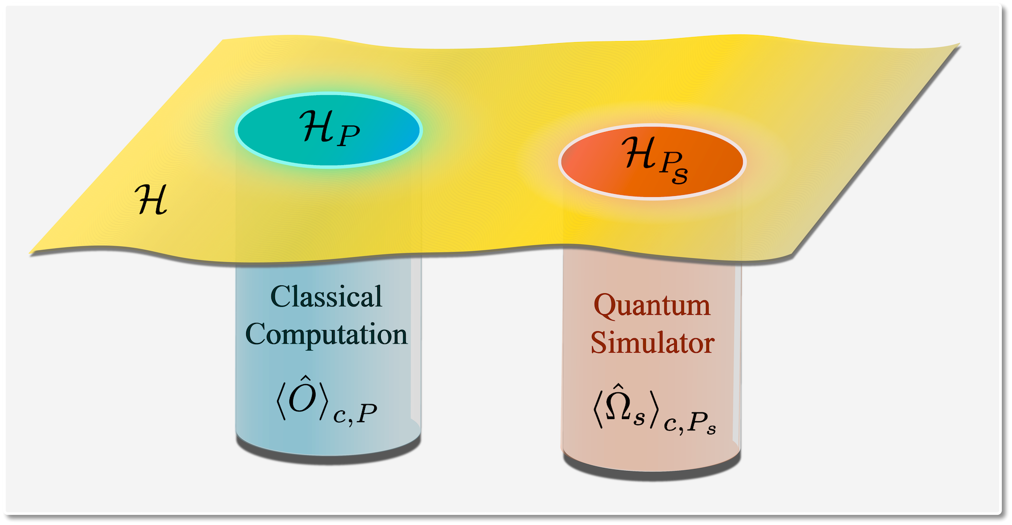
FIG. 2: [Upper Panel]: $\mathcal{H}_{P}$ (blue) and $\mathcal{H}_{\text{$P_{\scalebox{1.15}{$s$}}$}}$ (orange) are subspaces of $\mathcal{H}$ (yellow) that are specified by $\hat{H}$ and $\hat{H}_{s}$. [Lower Panel]: Classical computation and quantum simulation are used to probe the equivalence of $\mathcal{H}_{P}$ and $\mathcal{H}_{\text{$P_{\scalebox{1.15}{$s$}}$}}$.

This is accomplished by sampling from the coarse-grained benchmarking states with a uniform probability:

$${\braket{\hat{\Omega}_{s}}_{{c,\text{{\hbox{P_{\scalebox{1.0}{}}}}}}}}\approx\frac{1}{N_{\text{samp}}}\sum_{i=1}^{N_{\text{samp}}}\bra{\psi^{(i)}_{b}}\hat{\Omega}_{s}\ket{\psi^{(i)}_{b}}$$ (II.47)

If $\mathcal{H}_{P}=\mathcal{H}_{\text{$P_{\scalebox{1.15}{$s$}}$}}$, the projected coarse-grained orthodox expectation value will equal the projected coarse-grained simulated time-averaged expectation value (Figure 2).

III Energy-Window Time-Averaging

Energy-window Time-Averaging (ETA) is a coarse-grained benchmarking procedure. Coarse-grained benchmarking can be represented schematically in three stages:

1. Projection: Establish a subspace mapping.

2. Standardization: Sample benchmark orthodox mixed states to establish a standard of comparison.

3. Arbitration: Sample coarse-grained benchmarking states to establish a simulation diagnostic.

III.1 Projection

Both ETA-Variant I and ETA-Variant II require an energy-window $\Delta_{\epsilon}$ to perform projection:

$$\epsilon_{\text{min}}<\mathcal{E}<\epsilon_{\text{max}},\ \forall\mathcal{E}\in\Delta_{\epsilon}$$ (III.1)

III.1.1 Variant I

In ETA-Variant I, the subspace mapping uses the expectation value of the Hamiltonian to define a subset $\mathcal{H}_{P}^{(I)}\in\mathcal{H}$. States with average energies that fall within the energy-window are members of the subset (Figure 4):

$$\bra{\psi}\hat{H}\ket{\psi}\in\Delta_{\epsilon},\ \forall\ket{\psi}\in\mathcal{H}^{(I)}_{P}$$ (III.2)

III.1.2 Variant II

In ETA-Variant II, the subspace mapping uses the eigenstates of the Hamiltonian to define a subspace $\mathcal{H}_{P}^{(II)}\in\mathcal{H}$. States with eigenvalues inside the energy-window are members of the subspace (Figure 4):

$$\hat{H}\ket{\alpha_{i}}=\mathcal{E}_{\scalebox{0.8}{$\alpha$}_{\scalebox{0.7}{$i$}}} \ket{\alpha_{i}},\ \mathcal{E}_{\scalebox{0.8}{$\alpha$}_{\scalebox{0.7}{$i$}}}\in\Delta_{\epsilon}$$ (III.3)

$$\mathcal{H}^{(II)}_{P}=\overline{\text{span}}\big{\{}\kern 1.00006pt \ket{\alpha_{1}},\kern 1.00006pt\ket{\alpha_{2}},\ \scalebox{1.12}{$\ldots$}\ \big{\}}$$ (III.4)

III.1.3 Energy-Window Selection

To select an energy-window, the extremum energy eigenvalues must be determined. The extremizing orthodox mixed state is the following:

$${\tilde{\rho}_{\text{ext}}^{(\tau)}=\frac{1}{\mathcal{Z}}\kern 1.66672pt\text{{\hbox{e^{\kern 0.70007pt\scalebox{0.92}{}}}}}}$$ (III.5)

Taking $\tau\rightarrow-\infty$ results in the minimum energy:

$$\lim_{\tau\rightarrow-\infty}\text{Tr}\Big{[}\rho_{\text{ext}}^{(\tau)}\kern 1.66672pt\hat{H}\Big{]}=\mathcal{E}_{\text{min}}$$ (III.6)

Taking $\tau\rightarrow\infty$ results in the maximum energy:

$$\lim_{\tau\rightarrow\infty}\text{Tr}\Big{[}\tilde{\rho}_{\text{ext}}^{(\tau)}\kern 1.66672pt\hat{H}\Big{]}=\mathcal{E}_{\text{max}}$$ (III.7)

Viable energy-windows have the following restriction:

$$\mathcal{E}_{\text{min}}<\epsilon_{\text{min}}<\epsilon_{\text{max}}<\mathcal{E}_{\text{max}}$$ (III.8)

III.2 Standardization

In ETA-Variant I and ETA-Variant II, benchmark orthodox mixed states are generated to establish a standard of comparison.

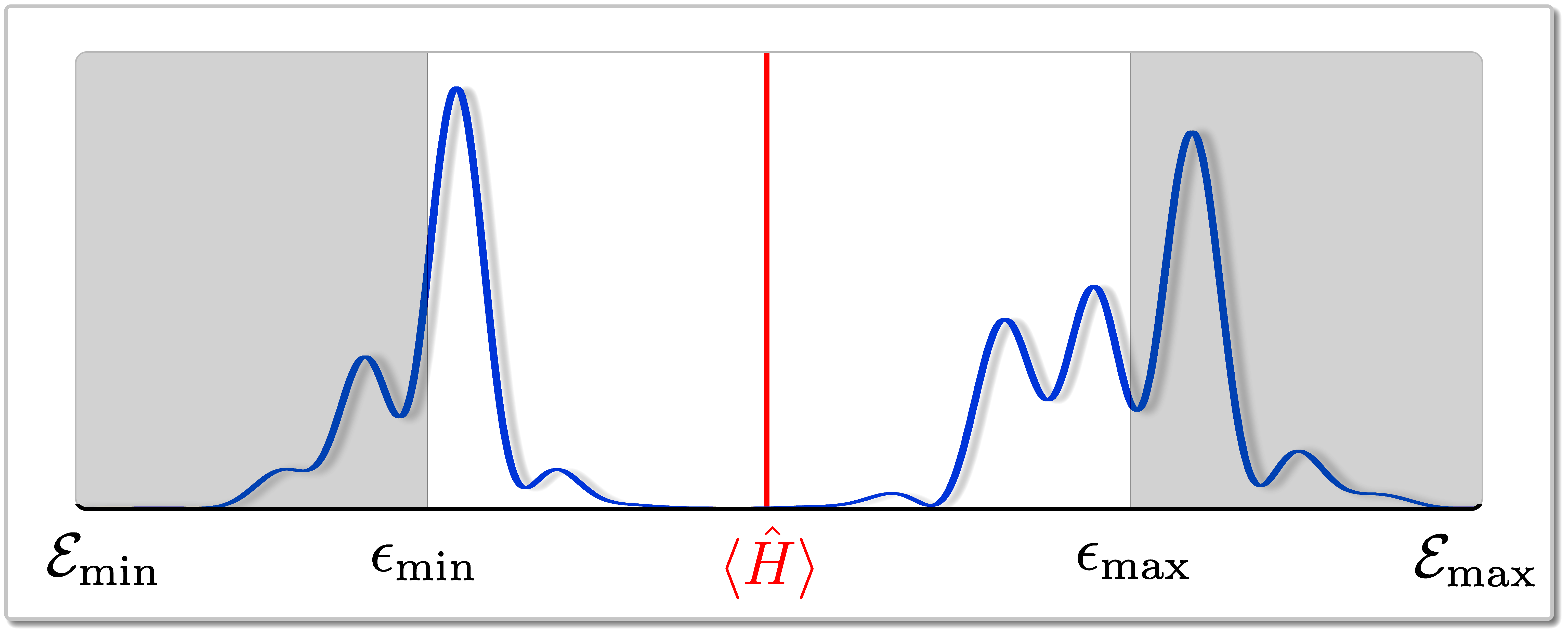
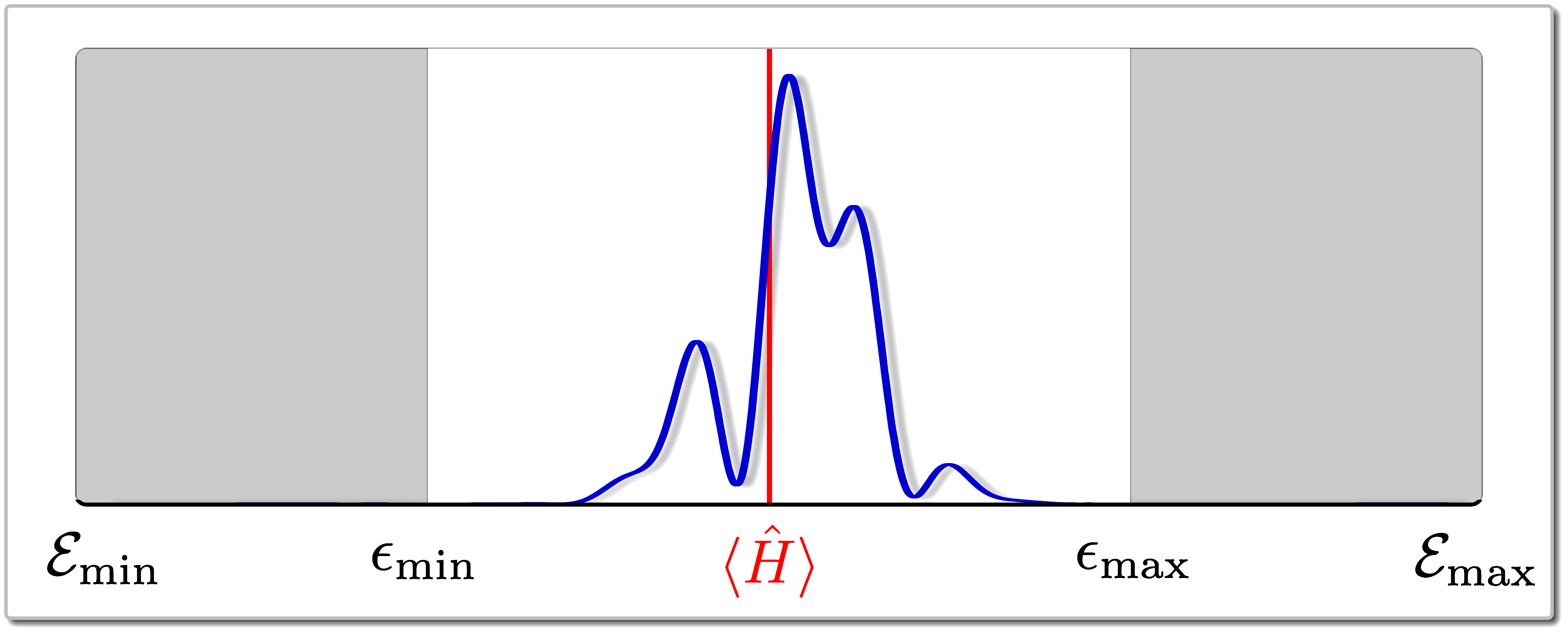
FIG. 3: The energy-eigenstate decomposition (blue) of a state in the ETA-Variant I subset, has an average energy (red) that falls within the energy-window (white).

FIG. 4: The energy-eigenstate decomposition (blue) of a state in the ETA-Variant II subspace, is zero outside of the energy-window (white).

III.2.1 Variant I

In ETA-Variant I, orthodox mixed states are generated pseudo-randomly using positive-real functions $f_{\gamma}(x)$.

These functions are normalized over the extremum eigenvalues:

$$\int_{\mathcal{E}_{\text{min}}}^{\mathcal{E}_{\text{max}}}d\mathcal{E}\ f_{\gamma}(\mathcal{E})=1$$ (III.9)

The average energy of the functions lies within the energy window:

$$\int_{\mathcal{E}_{\text{min}}}^{\mathcal{E}_{\text{max}}}d\mathcal{E}\ f_{\gamma}(\mathcal{E})\kern 1.66672pt\mathcal{E}\kern 1.66672pt\in\kern 1.66672pt\Delta_{\epsilon}$$ (III.10)

An orthodox mixed state is constructed from a chosen function $f_{\scalebox{0.8}{$\gamma^{\prime}$}}(x)$. If $\braket{\hat{H}}$ falls within the energy-window, a benchmark orthodox mixed state was generated:

$$\kern-3.00003pt\kern-1.49994pt\braket{\hat{H}}\in\Delta_{\epsilon},$$

$$\tilde{\rho}(f_{\scalebox{0.8}{$\gamma^{\prime}$}})\kern 1.66672pt \in\kern 1.66672pt\Big{\{}\mathcal{H}\otimes\text{$\mathcal{H}^{*}$}\Big{\}}^{(I)}_{P}$$ (III.11)

III.2.2 Variant II

In ETA-Variant II, gaussian orthodox mixed states are generated pseudo-randomly:

$$\tilde{\rho}_{g}(\epsilon,\sigma) =\frac{1}{\mathcal{Z}}\sum_{\alpha}\scalebox{1.1}{$e$}^{-\Big{(}\scalebox{1.3}{$\frac{\mathcal{E}_{\alpha}-\epsilon}{\sigma}$}\Big{)}^{2}}\ket{\alpha}\kern-1.49994pt\bra{\alpha}$$ (III.12)

To increase the likelihood that a benchmark orthodox mixed state is generated, $\epsilon$ and $\sigma$ are constrained:

$$\epsilon\in\Delta_{\epsilon}\ \ \kern 1.66672pt$$ (III.13)

$$e^{-\Big{(}\scalebox{1.2}{$\frac{\epsilon_{\text{min}}-\epsilon}{\sigma}$}\Big{)}^{2}} \ll 1$$ (III.14)

$$e^{-\Big{(}\scalebox{1.2}{$\frac{\epsilon_{\text{max}}-\epsilon}{\sigma}$}\Big{)}^{2}} \ll 1$$ (III.15)

A gaussian orthodox mixed state is constructed from the chosen parameters $(\epsilon,\sigma)$. The expectation value of the Hamiltonian and its variance are determined:

$$\text{Var}(\hat{H})=\braket{\text{{\hbox{\hat{H}^{\kern 0.70007pt2}}}}}-\text{{\hbox{\braket{\hat{H}}^{\kern-1.49994pt2}}}}$$ (III.16)

If $\braket{\hat{H}}$ and its uncertainty fall outside the energy-window, a benchmark orthodox mixed state was not generated:

$$\braket{\hat{H}}\pm\sqrt{\text{Var}(\hat{H})}\kern 1.66672pt\notin\kern 1.66672pt\Delta_{\epsilon},$$

$$\kern 1.00006pt\tilde{\rho}_{g}(\epsilon,\kern 1.66672pt\sigma)\kern 1.66672pt\notin\kern 1.66672pt\Big{\{}\mathcal{H}\otimes\text{$\mathcal{H}^{*}$}\Big{\}}^{(II)}_{P}$$ (III.17)

III.3 Arbitration

In ETA-Variant I and ETA-Variant II, coarse-grained benchmarking states are prepared to establish a simulation diagnostic.

III.3.1 State Preparation

Variant I

In ETA-Variant I, coarse-grained benchmarking states are prepared using a variational hybrid quantum-classical algorithm [14]. These algorithms seek to use classical optimization to prepare pure states that minimize a cost-function [15].

A set of pure states is identified by applying a class of unitary transformations to an edge state $\ket{\psi_{e}}$:

$$\Ket{\psi_{e}^{(\vec{p})}}=\text{{\hbox{\hat{U}^{(\vec{p})}}}}\Ket{\psi_{e}}$$ (III.18)

The cost-function is the absolute difference between the expectation value of the simulation Hamiltonian and the center of the energy-window:

$$\mathcal{C}_{e}(\vec{p})=\Bigg{|}\Bra{\psi_{e}^{(\vec{p})}}\hat{H}_{s}\Ket{\psi_{e}^{(\vec{p})}}-\Big{(}\frac{\epsilon_{\text{max}}+\epsilon_{\text{min}}}{2}\Big{)}\Bigg{|}$$ (III.19)

An edge state is generated pseudo-randomly, and the variational hybrid quantum-classical algorithm is allowed to run to completion. During the course of the algorithm, coarse-grained benchmarking states may be generated.

The accessible coarse-grained benchmarking states are identified by the parameters $(e,\vec{p}_{b}$) for which the following condition holds:

$${\Bra{\psi_{e}^{(\vec{p}_{b})}}\hat{H}_{s}\Ket{\psi_{e}^{(\vec{p}_{b})}}\in\Delta_{\epsilon},\ \forall\kern 1.00006pt\Ket{\psi_{e}^{(\vec{p}_{b})}}\in\mathcal{H}^{(I)}_{{\text{{\hbox{P_{\scalebox{1.0}{}}}}}}}}$$ (III.20)

Variant II

In ETA-Variant II, coarse-grained benchmarking states are prepared using an adiabatic quantum simulation algorithm [16]. These algorithms seek to prepare eigenstates of a Hamiltonian [17, 18].

An initializing Hamiltonian $\hat{H}_{i}$ has known eigenstates $\ket{\text{$\phi^{(i)}_{n}$}}$:

$$\hat{H}_{i}\Ket{\text{{\hbox{\phi^{(i)}_n}}}}=\text{{\hbox{\lambda_n^{(i)}}}}\Ket{\text{{\hbox{\phi^{(i)}_n}}}}$$ (III.21)

The annealing time $\tau$ parametrizes the preparation Hamiltonian:

$$\hat{H}^{\scalebox{0.8}{$(i,\tau)$}}_{p}\kern-1.00006pt\scalebox{0.9}{$(t)$}=\Big{\{}\hat{H}_{s}-\hat{H}_{i}\Big{\}}\big{(}t/\tau\big{)}+\hat{H}_{i}$$ (III.22)

A set of pure states is identified by time-evolving a known eigenstate under preparation Hamiltonians:

$$\kern-3.00003pt\qquad\kern 1.66672pt\Ket{\text{$\psi^{(\scalebox{0.8}{$i,\tau$})}_{n}$}}=\text{$\hat{U}^{\scalebox{0.8}{$(i,\tau)$}}$}\Ket{\text{$\phi^{(i)}_{n}$}}$$ (III.23)

$$\raisebox{-3.99994pt}{\text{$\hat{U}^{\scalebox{0.8}{$(i,\tau)$}}$} }\raisebox{-3.00003pt}{=}\ \raisebox{-3.99994pt}{\scalebox{1.03}{$\mathcal{T}$}}\kern 1.66672pt\scalebox{0.9}{$\Bigg{(}$}\kern 1.66672pt\raisebox{-5.0pt}{\scalebox{1.1}{$e$}}^{\kern-1.04996pt-i\scalebox{1.0}{$\scalebox{1.2}{$\int$}_{\kern-1.47002pt0}^{\tau}dt^{{}^{\prime}}\ \hat{H}^{\scalebox{0.8}{$(i,\tau)$}}_{p}\kern-1.04996pt\scalebox{0.9}{$(t^{{}^{\prime}})$}$}}\kern 1.66672pt\scalebox{0.9}{$\Bigg{)}$}$$ (III.24)

The simulation eigenvalues $E_{n}^{(\scalebox{0.8}{$i,\tau$})}$ are defined as follows:

$$\qquad\ \hat{H}_{s}\Ket{\text{$\text{$\alpha^{s}_{k}$}$}}=\text{$\mathcal{E}^{s}_{\scalebox{0.8}{$\alpha$}_{\scalebox{0.7}{$k$}}}$}\Ket{\text{$\text{$\alpha^{s}_{k}$}$}}$$ (III.25)

$$\Braket{\text{$\text{$\alpha^{s}_{k}$}$}\kern 1.00006pt}{\kern 1.00006pt\text{$\psi^{(\scalebox{0.8}{$i,\tau$})}_{n}$}}\neq 0,\ \ \forall\kern 1.00006pt\text{$\mathcal{E}^{s}_{\scalebox{0.8}{$\alpha$}_{\scalebox{0.7}{$k$}}}$}\in E_{n}^{(\scalebox{0.8}{$i,\tau$})}$$ (III.26)

After specifying an initializing Hamiltonian, both the annealing time and the known eigenstate are chosen pseudo-randomly.

The accessible coarse-grained benchmarking states are identified by the parameters $(i,\tau_{b},n_{b})$ for which the following condition holds:

$$E_{n_{b}}^{(\scalebox{0.8}{$i,\tau_{b}$})}\in\Delta_{\epsilon},\ \forall\Ket{\text{$\psi^{(\scalebox{0.8}{$i,\tau_{b}$})}_{n_{b}}$}}\in\mathcal{H}^{(II)}_{\text{$P_{\scalebox{1.0}{$s$}}$}}$$ (III.27)

To determine if a coarse-grained benchmarking state was generated, quantum simulation is used to place a bound on the simulation eigenvalues of $\ket{\text{$\psi^{(\scalebox{0.8}{$i,\tau$})}_{n}$}}$.

The simulated expectation value is the following:

$$\kern-3.00003pt\braket{\hat{O}_{s}(t)} =\Bra{\text{$\psi^{(\scalebox{0.8}{$i,\tau$})}_{n}$}}\text{$e^{\scalebox{0.92}{$\kern 0.70004pti\hat{H}_{s}t$}}$}\kern 1.66672pt\hat{O}\kern 1.66672pt\text{$e^{-\scalebox{0.92}{$i\hat{H}_{s}t$}}$}\Ket{\text{$\psi^{(\scalebox{0.8}{$i,\tau$})}_{n}$}}$$ (III.28)

$$=\sum_{\text{$\alpha^{s}$}\kern-1.04996pt,\kern 0.70004pt\text{$\beta^{s}$}}\text{$c^{*}_{\text{$\alpha^{s}$}}$}\kern 1.00006pt\text{$c_{\text{$\beta^{s}$}}$}\bra{\text{$\alpha^{\kern-0.70004pts}$}}\hat{O}\ket{\text{$\beta^{s}$}}\ \text{$e^{-\scalebox{0.92}{$it\big{(}\mathcal{E}^{s}_{\beta}-\mathcal{E}^{s}_{\alpha}\big{)}$}}$}$$ (III.29)

$$=\sum_{\text{$\alpha^{s}$}\kern-1.04996pt,\kern 0.70004pt\text{$\beta^{s}$}}\text{$\mathcal{D}_{\kern-1.04996pt\text{$\alpha^{s}$}\kern-1.04996pt,\kern 0.70004pt\text{$\beta^{s}$}}$}\ \text{$e^{-\scalebox{0.92}{$it\big{(}\mathcal{E}^{s}_{\beta}-\mathcal{E}^{s}_{\alpha}\big{)}$}}$}$$ (III.30)

The Fourier transform of the simulated expectation value is the following:

$$\braket{\hat{O}_{s}(\omega)} =\int_{-\infty}^{\infty}dt\ \text{$e^{-\scalebox{0.85}{$i\omega t$}}$}\braket{\hat{O}_{s}(t)}$$ (III.31)

$$=\sum_{\text{$\alpha^{s}$}\kern-1.04996pt,\kern 0.70004pt\text{$\beta^{s}$}}\text{$\mathcal{D}_{\kern-1.04996pt\text{$\alpha^{s}$}\kern-1.04996pt,\kern 0.70004pt\text{$\beta^{s}$}}$}\ \delta\Big{\{}\omega-\Big{(}\mathcal{E}^{s}_{\alpha}-\mathcal{E}^{s}_{\beta}\Big{)}\Big{\}}$$ (III.32)

$$=\sum_{\text{$\alpha^{s}$}\kern-1.04996pt,\kern 0.70004pt\text{$\beta^{s}$}}\text{$\mathcal{D}_{\kern-1.04996pt\text{$\alpha^{s}$}\kern-1.04996pt,\kern 0.70004pt\text{$\beta^{s}$}}$}\ \delta\Big{\{}\omega-\Delta^{\kern-1.04996pts}_{\text{$\alpha^{s}$}\kern-1.04996pt,\kern 0.70004pt\text{$\beta^{s}$}}\Big{\}}$$ (III.33)

The Fourier transform is peaked at the energy gaps ($\Delta^{\kern-0.94496pts}_{\text{$\alpha^{s}$}\kern-0.94496pt,\kern 0.63004pt\text{$\beta^{s}$}}$) of the simulation eigenvalues. The peaks are discernible if $\bra{\text{$\alpha^{\kern-0.63004pts}$}}\hat{O}\ket{\text{$\beta^{s}$}}\neq 0$.

The maximum energy-gap $\Delta^{\kern-0.94496pts}_{\text{max}}$ can be used to place a bound on the simulation eigenvalues:

$$\braket{\hat{H}_{s}}-\Delta^{\kern-1.04996pts}_{\text{max}}\leq\ E_{n}^{(\scalebox{0.8}{$i,\tau$})}\leq\braket{\hat{H}_{s}}+\Delta^{\kern-1.04996pts}_{\text{max}}$$ (III.34)

If the simulation eigenvalue bound falls within the energy-window, a coarse-grained benchmarking state was prepared:

$${\braket{\hat{H}_{s}}\pm\Delta^{\kern-1.04996pts}_{\text{max}}\in\Delta_{\epsilon},\ \kern 1.66672pt\Ket{\text{{\hbox{\psi^{(i,\tau)}_n}}}}\in\mathcal{H}^{(II)}_{{\text{{\hbox{P_{\scalebox{1.0}{}}}}}}}}$$ (III.35)

III.3.2 Time-Averaging

In ETA-Variant I and ETA-Variant II, the simulated time-averaged expectation values of the coarse-grained benchmarking states must be estimated.

The simulated expectation value averaged over time $t_{a}$ is the following:

$$\braket{\hat{O}_{s}}_{\text{ave}} =\frac{1}{t_{a}}\int_{0}^{t_{a}}dt^{{}^{\prime}}\ \braket{\hat{O}_{s}(t^{{}^{\prime}})}$$

$$=\sum_{\text{$\alpha^{s}$}\kern-1.04996pt,\kern 0.70004pt\text{$\beta^{s}$}}\text{$\mathcal{D}_{\kern-1.04996pt\text{$\alpha^{s}$}\kern-1.04996pt,\kern 0.70004pt\text{$\beta^{s}$}}$}\ \frac{1}{t_{a}}\int_{0}^{t_{a}}dt^{{}^{\prime}}\ \text{$e^{\kern 0.70004pt\scalebox{0.92}{$it^{{}^{\prime}}\big{(}\Delta^{\kern-0.73497pts}_{\text{$\alpha^{s}$}\kern-0.73497pt,\kern 0.49002pt\text{$\beta^{s}$}}\big{)}$}}$}$$ (III.36)

The simulated time-averaged expectation value is well-approximated when $t_{a}$ is much larger than the maximum period, which is set by the minimum energy-gap $\Delta^{\kern-0.94496pts}_{\text{min}}$:

$$t_{a}\gg\frac{2\pi}{\Delta^{\kern-1.04996pts}_{\text{min}}}>\frac{2\pi}{\Delta^{\kern-1.04996pts}_{\text{max}}},$$

$$\ \ \ \braket{\hat{O}_{s}}_{\text{ave}}\approx\braket{\hat{\Omega}_{s}}$$ (III.37)

To resolve the dynamics, the simulated expectation value must be sampled faster than the aliasing time, which is set by the maximum energy-gap [41, 42, 43]:

$$t_{samp}<\frac{\pi}{\Delta^{\kern-1.04996pts}_{\text{max}}}$$ (III.38)

When $\hat{H}_{s}\rightarrow\hat{H}$, the maximum energy-gap is upper-bounded by the energy breadth:

$$\Delta_{B}=\mathcal{E}_{\text{max}}-\mathcal{E}_{\text{min}}$$ (III.39)

The energy breadth is used to place constraints on the time-averaging parameters:

$$t_{\text{samp}}<\frac{\pi}{\Delta_{B}}$$ (III.40)

$$t_{a}\gg\frac{2\pi}{\Delta_{B}}$$ (III.41)

IV Numerical Implementation

To examine their efficacy, both ETA-Variant I and ETA-Variant II are applied to a Hamiltonian family.

IV.1 Benchmark Procedure

IV.1.1 Hamiltonian Family

The Hamiltonian family describes a particle of mass $m$, with a kinetic term that has a length-scale $a$:

$${{\hat{H}_{f}(\omega,\lambda)=-\frac{1}{2m}\Bigg{[}\frac{\text{{\hbox{e^{-\scalebox{0.92}{}}}}}}-\text{{\hbox{e^{\scalebox{0.92}{}}}}}}}{2a}\Bigg{]}^{2}+\frac{1}{2}\omega\kern 1.66672pt\text{{\hbox{\hat{x}^2}}}+\lambda\kern 1.66672pt\text{{\hbox{\hat{x}^3}}}$$ (IV.1)

The particle is confined to sites in a periodic lattice:

$$\text{sites}:\{-aN,\kern 1.00006pta\kern 0.70007pt(-N+1\kern 0.70007pt)\kern 0.70007pt,\ \scalebox{1.12}{{\hbox{\ldots}}}\ ,\kern 1.00006pta\kern 0.70007pt(N-1\kern 0.70007pt)\kern 0.70007pt,\kern 1.00006ptaN\}$$ (IV.2)

IV.1.2 Benchmark Hamiltonians

ETA is used to distinguish members of the Hamiltonian family from one another. $1001$-site lattices are used.

The target Hamiltonian has a fully quadratic potential:

$$\hat{H}=\hat{H}_{f}(\omega_{0},0)$$ (IV.3)

The corrupted Hamiltonians are generated by adjusting the cubic potential:

$$\hat{H}_{c}(\lambda)=\hat{H}_{f}(\omega_{0},\lambda)$$ (IV.4)

The corruption strength is the following quantity:

$$\eta=a\frac{\lambda}{\omega_{0}}$$ (IV.5)

IV.1.3 Energy-Window Selection

The target energy-range $\Delta_{\scalebox{0.8}{$\mathcal{E}$}}$ is defined as follows:

$$\mathcal{E}_{\text{min}}\leq\mathcal{E}\leq\mathcal{E}_{\text{max}},\ \forall\mathcal{E}\in\Delta_{\scalebox{0.8}{{\hbox{\mathcal{E}}}}}$$ (IV.6)

Three energy-windows are used during the benchmark:

Low-Range: bottom-15% of the target energy-range

Mid-Range: median-15% of the target energy-range

High-Range: top-15% of the target energy-range

IV.1.4 Observable Selection

The benchmark observable is the following:

$$\hat{X}_{a}=\text{{\hbox{\big{|}\kern 1.00006pt\hat{x}\kern 1.00006pt\big{|}^{1/3}}}}$$ (IV.7)

IV.1.5 Standardization

To establish a standard of comparison, $10^{4}$ benchmark orthodox mixed states are generated. A bootstrapping algorithm is used for statistical analysis [44, 45, 46].

IV.1.6 Arbitration

To establish a simulation diagnostic, $10^{4}$ coarse-grained benchmarking states are generated. A bootstrapping algorithm is used for statistical analysis.

IV.2 Numerical Results

IV.2.1 Low-Range Window

Variant I: ETA-Variant I positively benchmarks the target Hamiltonian. ETA-Variant I negatively benchmarks $3$ out of $5$ corrupted Hamiltonians (Figure 5).

Variant II: ETA-Variant II positively benchmarks the target Hamiltonian. ETA-Variant II negatively benchmarks $5$ out of $5$ corrupted Hamiltonians (Figure 6).

IV.2.2 Mid-Range Window

Variant I: ETA-Variant I positively benchmarks the target Hamiltonian. ETA-Variant I negatively benchmarks $5$ out of $5$ corrupted Hamiltonians (Figure 7).

Variant II: ETA-Variant II positively benchmarks the target Hamiltonian. ETA-Variant II negatively benchmarks $5$ out of $5$ corrupted Hamiltonians (Figure 8).

IV.2.3 High-Range Window

Variant I: ETA-Variant I positively benchmarks the target Hamiltonian. ETA-Variant I negatively benchmarks $5$ out of $5$ corrupted Hamiltonians (Figure 9).

Variant II: ETA-Variant II positively benchmarks the target Hamiltonian. ETA-Variant II negatively benchmarks $5$ out of $5$ corrupted Hamiltonians (Figure 10).

V Appendix: Monte-Carlo Methods

Monte-Carlo techniques are a class of algorithms that employ successive random sampling [47]. In particular, Markov-chain Monte-Carlo methods approximate sampling from a target probability distribution by recording the output of a stochastic numerical simulation [48, 49, 50, 51].

As the simulation time $\tau_{s}$ tends to infinity, the simulated distribution recovers the target distribution. The rate of convergence is independent of dimension: $\sim\mathcal{O}(1/\sqrt{\tau_{s}})$ [52]. The classical computations required for this work are tractable [53], even if quantum simulation is unfeasible due to the Hilbert space dimension [9, 54, 55, 56, 57, 58].

VI Acknowledgements

 

All of us, like sheep, have strayed away;
we have left God’s paths to follow our own.
Yet the Lord laid on Him the sins of us all.

-Isaiah 53:6

$-AMDG-$

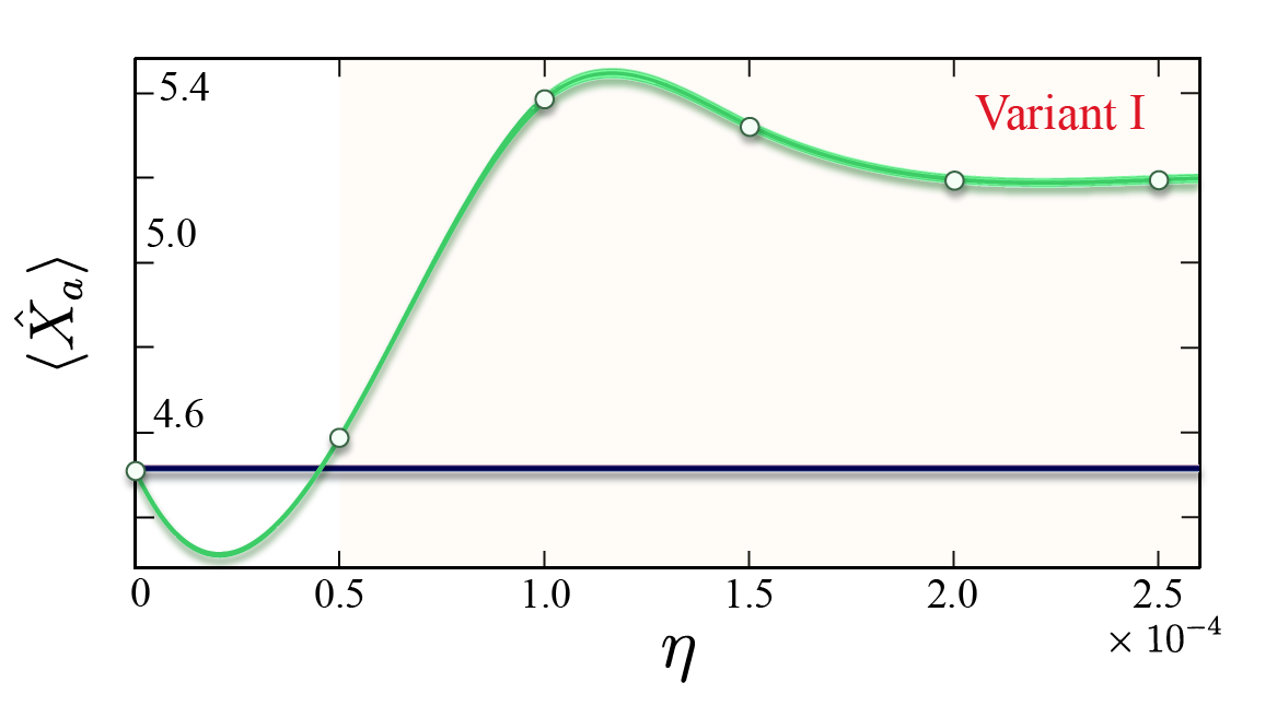
FIG. 5: Low-Range: The standard of comparison for the target Hamiltonian is determined using classical computing resources (blue curve). It is contrasted against the simulation diagnostic for the corrupted Hamiltonians (green curve).

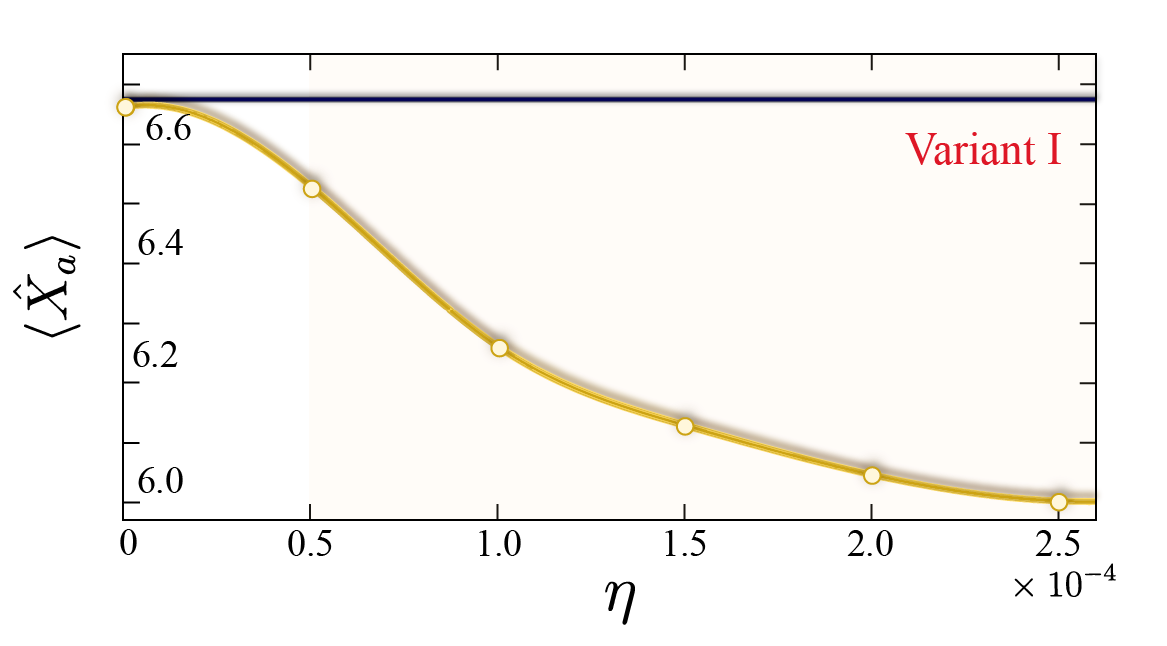
FIG. 7: Mid-Range: The standard of comparison for the target Hamiltonian is determined using classical computing resources (blue curve). It is contrasted against the simulation diagnostic for the corrupted Hamiltonians (yellow curve).

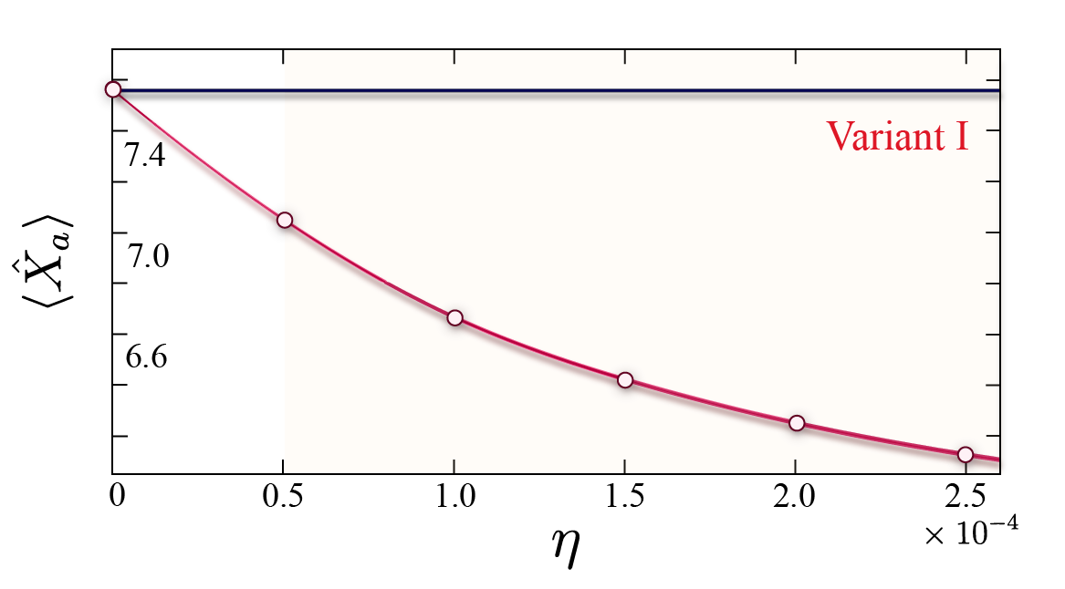
FIG. 9: High-Range: The standard of comparison for the target Hamiltonian is determined using classical computing resources (blue curve). It is contrasted against the simulation diagnostic for the corrupted Hamiltonians (red curve).

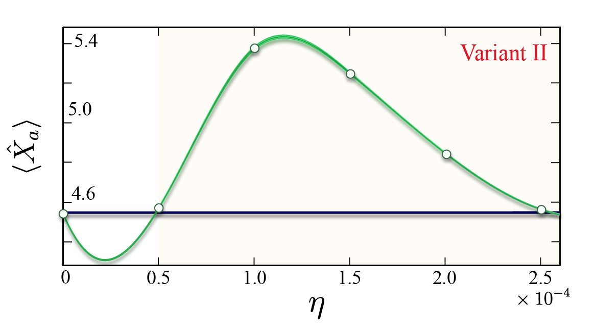
FIG. 6: Low-Range: The standard of comparison for the target Hamiltonian is determined using classical computing resources (blue curve). It is contrasted against the simulation diagnostic for the corrupted Hamiltonians (green curve).

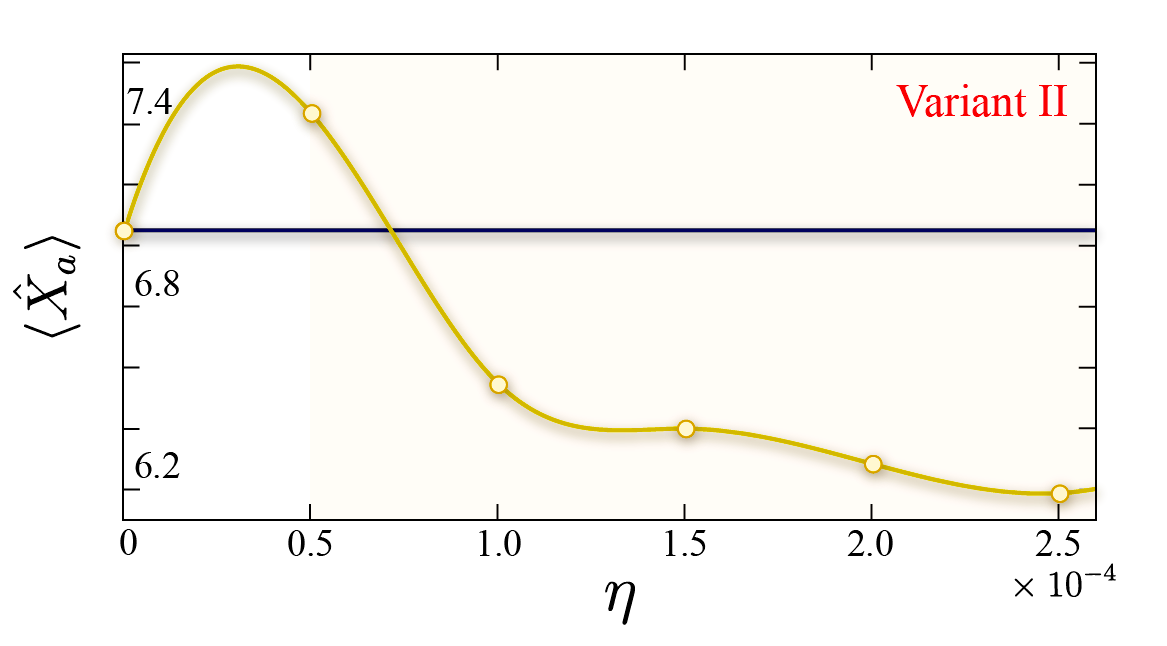
FIG. 8: Mid-Range: The standard of comparison for the target Hamiltonian is determined using classical computing resources (blue curve). It is contrasted against the simulation diagnostic for the corrupted Hamiltonians (yellow curve).

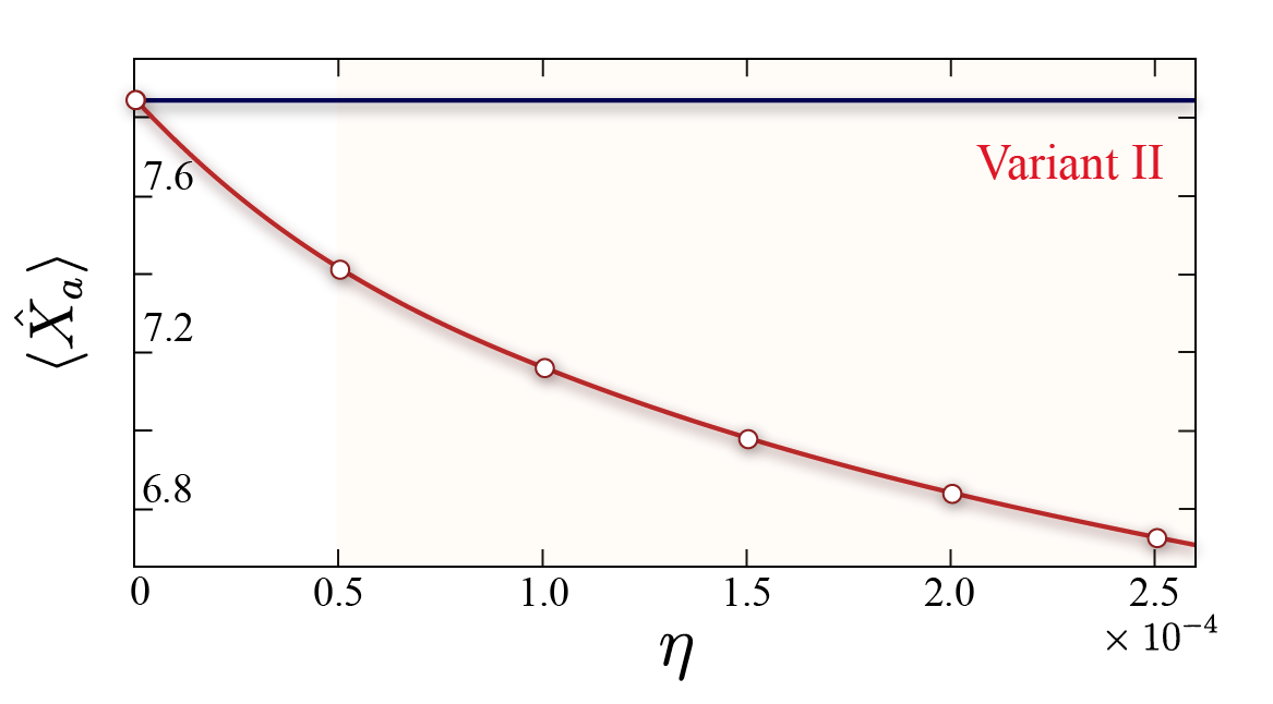
FIG. 10: High-Range: The standard of comparison for the target Hamiltonian is determined using classical computing resources (blue curve). It is contrasted against the simulation diagnostic for the corrupted Hamiltonians (red curve).

References

- Schrödinger [1926] E. Schrödinger, Quantization as an eigenvalue problem, Annalen der Physik 384, 361 (1926).
- Neumann [1927] J. v. Neumann, Probabilistic theory of quantum mechanics, Nachrichten von der Gesellschaft der Wissenschaften zu Göttingen, Mathematisch-Physikalische Klasse 1927, 245 (1927).
- Landau [1927] L. Landau, The damping problem in quantum mechanics, in Collected Papers of L.D. Landau (Pergamon, 1927) Chap. 2, pp. 8–18.
- Nielsen and Chuang [2011a] M. A. Nielsen and I. L. Chuang, Quantum computation and quantum information (Cambridge University Press, 2011) pp. 98–108.
- Fubini [1904] G. Fubini, On the metrics defined by a hermitian form, Office graf. C. Ferrari (1904).
- Study [1905] E. Study, Shortest routes in a complex area, Mathematische Annalen 60, 321 (1905).
- Haar [1933] A. Haar, The standard in the theory of continuous groups, Annals of Mathematics 34, 147 (1933).
- Boya et al. [2003] L. J. Boya, E. Sudarshan, and T. Tilma, Volumes of compact manifolds, Reports on Mathematical Physics 52, 401 (2003).
- Feynman [1982] R. P. Feynman, Simulating physics with computers, International Journal of Theoretical Physics 21, 467 (1982).
- Manin [1980] Y. I. Manin, Computable and uncomputable, Sovetskoye Radio, Moscow (1980).
- Turing [1937] A. M. Turing, On computable numbers, with an application to the decision problem, Proceedings of the London Mathematical Society s2-42, 230 (1937).
- Feynman [1948] R. P. Feynman, Space-time approach to non-relativistic quantum mechanics, Rev. Mod. Phys. 20, 367 (1948).
- Nielsen and Chuang [2011b] M. A. Nielsen and I. L. Chuang, Quantum computation and quantum information (Cambridge University Press, 2011) pp. 70–72.
- Peruzzo et al. [2014] A. Peruzzo, J. McClean, P. Shadbolt, M.-H. Yung, X.-Q. Zhou, P. J. Love, A. Aspuru-Guzik, and J. L. O’Brien, A variational eigenvalue solver on a photonic quantum processor, Nature Communications 5, 4213 (2014).
- McClean et al. [2016] J. R. McClean, J. Romero, R. Babbush, and A. Aspuru-Guzik, The theory of variational hybrid quantum-classical algorithms, New Journal of Physics 18, 023023 (2016).
- Farhi et al. [2000] E. Farhi, J. Goldstone, S. Gutmann, and M. Sipser, Quantum Computation by Adiabatic Evolution, arXiv e-prints , quant-ph/0001106 (2000), arXiv:quant-ph/0001106 [quant-ph] .
- Born and Fock [1928] M. Born and V. Fock, Proof of the adiabatic theorem, Zeitschrift für Physik 51, 165 (1928).
- Kato [1950] T. Kato, On the adiabatic theorem of quantum mechanics, Journal of the Physical Society of Japan 5, 435 (1950).
- Deutsch [1991] J. M. Deutsch, Quantum statistical mechanics in a closed system, Phys. Rev. A 43, 2046 (1991).
- Srednicki [1994] M. Srednicki, Chaos and quantum thermalization, Phys. Rev. E 50, 888 (1994).
- Rigol et al. [2008] M. Rigol, V. Dunjko, and M. Olshanii, Thermalization and its mechanism for generic isolated quantum systems, Nature 452, 854 (2008).
- Cassidy et al. [2011] A. C. Cassidy, C. W. Clark, and M. Rigol, Generalized thermalization in an integrable lattice system, Phys. Rev. Lett. 106, 140405 (2011).
- Rigol and Srednicki [2012] M. Rigol and M. Srednicki, Alternatives to eigenstate thermalization, Phys. Rev. Lett. 108, 110601 (2012).
- Müller et al. [2015] M. P. Müller, E. Adlam, L. Masanes, and N. Wiebe, Thermalization and canonical typicality in translation-invariant quantum lattice systems, Communications in Mathematical Physics 340, 499 (2015).
- Xu et al. [2019] S. Xu, X. Li, Y.-T. Hsu, B. Swingle, and S. Das Sarma, Butterfly effect in interacting aubry-andre model: Thermalization, slow scrambling, and many-body localization, Phys. Rev. Research 1, 032039 (2019).
- Richter et al. [2020] J. Richter, A. Dymarsky, R. Steinigeweg, and J. Gemmer, Eigenstate thermalization hypothesis beyond standard indicators: Emergence of random-matrix behavior at small frequencies, Phys. Rev. E 102, 042127 (2020).
- Kuno et al. [2020] Y. Kuno, T. Mizoguchi, and Y. Hatsugai, Flat band quantum scar, Phys. Rev. B 102, 241115 (2020).
- Schuckert and Knap [2020] A. Schuckert and M. Knap, Probing eigenstate thermalization in quantum simulators via fluctuation-dissipation relations, Phys. Rev. Research 2, 043315 (2020).
- Cipolloni et al. [2020] G. Cipolloni, L. Erdős, and D. Schröder, Eigenstate Thermalization Hypothesis for Wigner Matrices, arXiv e-prints , arXiv:2012.13215 (2020), arXiv:2012.13215 [math.PR] .
- Noh [2021] J. D. Noh, Eigenstate thermalization hypothesis and eigenstate-to-eigenstate fluctuations, Phys. Rev. E 103, 012129 (2021).
- Huang [2021] Y. Huang, Finite-size scaling analysis of eigenstate thermalization, arXiv e-prints , arXiv:2103.01539 (2021), arXiv:2103.01539 [cond-mat.stat-mech] .
- Nakerst and Haque [2021] G. Nakerst and M. Haque, Eigenstate thermalization scaling in approaching the classical limit, Phys. Rev. E 103, 042109 (2021).
- Halataei [2021] S. M. H. Halataei, On eigenstate thermalization in the SYK chain model, arXiv e-prints , arXiv:2104.05291 (2021), arXiv:2104.05291 [hep-th] .
- Schönle et al. [2021] C. Schönle, D. Jansen, F. Heidrich-Meisner, and L. Vidmar, Eigenstate thermalization hypothesis through the lens of autocorrelation functions, Phys. Rev. B 103, 235137 (2021).
- Fritzsch and Prosen [2021] F. Fritzsch and T. Prosen, Eigenstate thermalization in dual-unitary quantum circuits: Asymptotics of spectral functions, Phys. Rev. E 103, 062133 (2021), arXiv:2103.11694 [cond-mat.stat-mech] .
- Balachandran et al. [2021] V. Balachandran, G. Benenti, G. Casati, and D. Poletti, From ETH to algebraic relaxation of OTOCs in systems with conserved quantities, arXiv e-prints , arXiv:2106.00234 (2021), arXiv:2106.00234 [cond-mat.stat-mech] .
- Decker et al. [2021] K. S. C. Decker, D. M. Kennes, and C. Karrasch, Many-body localization and the area law in two dimensions, arXiv e-prints , arXiv:2106.12861 (2021), arXiv:2106.12861 [cond-mat.dis-nn] .
- De Palma and Rouzé [2021] G. De Palma and C. Rouzé, Quantum concentration inequalities, arXiv e-prints , arXiv:2106.15819 (2021), arXiv:2106.15819 [quant-ph] .
- Khudorozhkov et al. [2021] A. Khudorozhkov, A. Tiwari, C. Chamon, and T. Neupert, Hilbert space fragmentation in a 2D quantum spin system with subsystem symmetries, arXiv e-prints , arXiv:2107.09690 (2021), arXiv:2107.09690 [cond-mat.str-el] .
- Mukherjee et al. [2021] B. Mukherjee, Z. Cai, and W. V. Liu, Constraint-induced breaking and restoration of ergodicity in spin-1 PXP models, Physical Review Research 3, 033201 (2021), arXiv:2104.00699 [quant-ph] .
- Whittaker [1915] E. Whittaker, On the functions which are represented by the expansions of the interpolation-theory, Proceedings of the Royal Society of Edinburgh 35, 181 (1915).
- Nyquist [1928] H. Nyquist, Certain topics in telegraph transmission theory, Transactions of the American Institute of Electrical Engineers 47, 617 (1928).
- Shannon [1949] C. Shannon, Communication in the presence of noise, Proceedings of the IRE 37, 10 (1949).
- Efron [1979] B. Efron, Bootstrap methods: Another look at the jackknife, Ann. Statist. 7, 1 (1979).
- Kunsch [1989] H. R. Kunsch, The jackknife and the bootstrap for general stationary observations, Ann. Statist. 17, 1217 (1989).
- Politis and Romano [1994] D. N. Politis and J. P. Romano, The stationary bootstrap, Journal of the American Statistical Association 89, 1303 (1994).
- Kroese et al. [2014] D. P. Kroese, T. Brereton, T. Taimre, and Z. I. Botev, Why the monte carlo method is so important today, WIREs Computational Statistics 6, 386 (2014).
- Metropolis et al. [1953] N. Metropolis, A. W. Rosenbluth, M. N. Rosenbluth, A. H. Teller, and E. Teller, Equation of state calculations by fast computing machines, The Journal of Chemical Physics 21, 1087 (1953).
- Hastings [1970] W. K. Hastings, Monte Carlo sampling methods using Markov chains and their applications, Biometrika 57, 97 (1970).
- Gilks and Wild [1992] W. R. Gilks and P. Wild, Adaptive rejection sampling for gibbs sampling, Journal of the Royal Statistical Society. Series C (Applied Statistics) 41, 337 (1992).
- Hill and Spall [2019] S. D. Hill and J. C. Spall, Stationarity and convergence of the metropolis-hastings algorithm: Insights into theoretical aspects, IEEE Control Systems Magazine 39, 56 (2019).
- Caflisch [1998] R. E. Caflisch, Monte carlo and quasi-monte carlo methods, Acta Numerica 7, 1 (1998).
- Cobham [1965] A. Cobham, The intrinsic computational difficulty of functions, North-Holland Publishing , 24 (1965).
- Lloyd [1996] S. Lloyd, Universal quantum simulators, Science 273, 1073 (1996).
- Nagaj [2010] D. Nagaj, Fast universal quantum computation with railroad-switch local Hamiltonians, Journal of Mathematical Physics 51, 062201 (2010), arXiv:0908.4219 [quant-ph] .
- Berry et al. [2015] D. W. Berry, A. M. Childs, and R. Kothari, Hamiltonian simulation with nearly optimal dependence on all parameters, arXiv e-prints , arXiv:1501.01715 (2015), arXiv:1501.01715 [quant-ph] .
- Hao Low and Chuang [2016] G. Hao Low and I. L. Chuang, Hamiltonian Simulation by Qubitization, arXiv e-prints , arXiv:1610.06546 (2016), arXiv:1610.06546 [quant-ph] .
- Haah et al. [2018] J. Haah, M. B. Hastings, R. Kothari, and G. Hao Low, Quantum algorithm for simulating real time evolution of lattice Hamiltonians, arXiv e-prints , arXiv:1801.03922 (2018), arXiv:1801.03922 [quant-ph] .