Deterministic particle flows for constraining SDEs

Abstract

Devising optimal interventions for diffusive systems often requires the solution of the Hamilton-Jacobi-Bellman (HJB) equation, a nonlinear backward partial differential equation (PDE), that is, in general, nontrivial to solve. Existing control methods either tackle the HJB directly with grid-based PDE solvers, or resort to iterative stochastic path sampling to obtain the necessary controls. Here, we present a framework that interpolates between these two approaches. By reformulating the optimal interventions in terms of logarithmic gradients (scores) of two forward probability flows, and by employing deterministic particle methods for solving Fokker-Planck equations, we introduce a novel fully deterministic framework that computes the required optimal interventions in one shot.

1 Introduction

Constrained diffusions and optimal control.

Consider the problem of imposing constraints $\mathcal{C}$ to the state of a stochastic system, whose unconstrained dynamics are described by a stochastic differential equation (SDE)

$$dX_{t}=f(X_{t},t)dt+\sigma dW_{t},$$ (1)

with drift $f(x,t)\in\mathcal{R}^{d}\times\mathcal{R}\rightarrow\mathcal{R}^{d}$ and diffusion coefficient $\sigma\in\mathcal{R}$. For a time interval $[0,\,T]$, the constraints $\mathcal{C}$ may pertain either the transient state of the system through a path-penalising function $U(x,t)\in\mathcal{R}^{d}\times\mathcal{R}\rightarrow\mathcal{R}$ for $t\leq T$, or its terminal state $X_{T}$ through the function $\chi(x)\in\mathcal{R}^{d}\rightarrow\mathcal{R}$.

One way to obtain the path probability measure $\mathbb{Q}$ of the constrained process is by reweighting paths $X_{0:T}$ generated from Eq.(1) over the interval $[0,\,T]$. Path weights result from the Radon–Nikodym derivative with respect to the path measure of the unconstrained process $\mathbb{P}_{f}$

$$\small\frac{d\mathbb{Q}}{d\mathbb{P}_{f}}(X_{0:T})=\frac{\chi(X_{T})}{Z}\exp\left[-\int_{0}^{T}U(X_{t},t)dt\right],$$ (2)

where $Z$ is a normalising constant.

How shall we modify the system of Eq.(1) to incorporate the desired constraints $\mathcal{C}$ into its dynamics, while also minimising the relative entropy between the path distributions of the constrained and unconstrained processes?

Problems of this form appear often in physics, biology, and engineering, and are relevant for calculation of rare event probabilities [1, 2], latent state estimation of partially observed systems [3, 4], or for precise manipulation of stochastic systems to target states [5, 6] with applications on artificial selection [7, 8], motor control [9], epidemiology, and more [10, 11, 12, 13, 14, 15]. Yet, although stochastic optimal control problems are prevalent in most scientific fields, their numerical solution remains computationally demanding for most practical problems.

The constrained process, defined by the weight of Eq.(2), can be also expressed as a diffusion process with the same diffusion $\sigma$, but with a modified time-dependent drift $g(x,t)$ [16, 17]. The computation of this drift adjustment or control $u(x,t)\doteq g(x,t)-f(x,t)$ amounts to solving a stochastic control problem to obtain the optimal control $u^{*}(x,t)$ that minimises the expected cost

$$\small\mathcal{J}(x,t)\doteq\min_{u}\mathbb{E}_{\mathbb{P}_{g}}\left[\int_{0}^{T}\left(\frac{1}{2\sigma^{2}}\|u(X_{t},t)\|^{2}+U(X_{t},t)\right)dt-\ln\chi(X_{T})\right].$$ (3)

The expectation $\mathbb{E}_{\mathbb{P}_{g}}$ is over paths induced by the constrained SDE $\;dX_{t}=g(X_{t},t)dt+\sigma dW_{t}.\;\;\;\ ({\color[rgb]{1,0,1}4})$
This control setting is known as Path Integral- or Kullback-Leibler-control (PI/KL-control)[4, 5, 18, 19]. Finding the exact optimal interventions for general stochastic control problems amounts to solving the HJB equation [20], a computationally demanding nonlinear PDE. Yet, for the PI-control problem, the logarithmic Hopf-Cole transformation [21], ie. ${\mathcal{J}(x,t)=-\log(\phi_{t}(x))}$, linearises the HJB equation [5], and the optimally adjusted drift becomes $$g(x,t)=f(x,t)+\sigma^{2}\nabla\ln\phi_{t}(x),$$ (5) $$\frac{\partial\phi_{t}(x)}{\partial t}+{\cal{L}}^{\dagger}_{f}\phi_{t}(x)-U(x,t)\phi_{t}(x)=0,$$ (6) where $\phi_{t}(x)$ is a solution to the backward PDE of Eq.(6) with terminal condition $\phi_{T}(x)=\chi(x)$, and $\mathcal{L}^{\dagger}_{f}\phi(x)\doteq f(x,t)\nabla\cdot\phi(x)+\frac{\sigma^{2}}{2}\nabla^{2}\phi(x)$ denotes the adjoint Fokker–Planck operator acting on $\phi(x)$.

The PDE of Eq.(6) is often treated either with grid based solvers [22, 23], or with iterative stochastic path sampling schemes  [19, 5, 24, 25]. Both approaches suffer, in general, from high computational complexity with increasing system dimension. (However note recent neural network advances towards this direction [26, 27].)

2 Method

Constrained diffusion densities from backward smoothing.

To avoid directly solving the backward PDE (Eq. (6)), we view the marginal density $q_{t}(x)$ of the constrained process as the smoothing density in an inference setting. By considering Eq.(2) as a likelihood function, and treating the constraints $U(x,t)$ and $\chi(x)$ as continuous time observations of the process $X_{t}$, the path measure $\mathbb{Q}$, i.e. the product of the a priori distribution $\mathbb{P}_{f}$ with the likelihood, can be interpreted as the posterior distribution over paths that account for the observations as soft constraints. Thus, in a similar vein to the forward–backward smoothing algorithms for hidden Markov models [28, 29], we factorise the marginal density into two terms that account for past and future constraints separately

$$q_{t}(x)\propto\rho_{t}(x)\phi_{t}(x).$$ (7)

The density $\rho_{t}(x)$ satisfies the forward filtering equation with initial condition $\rho_{0}(x)$ (Eq.(8)), while the marginal constrained density $q_{t}(x)$ fulfils a Fokker–Planck equation (Eq.(9)) $$\frac{\partial\rho_{t}(x)}{\partial t}={\cal{L}}_{f}\rho_{t}(x)-U(x,t)\rho_{t}(x),$$ (8) $$\frac{\partial q_{t}(x)}{\partial t}={\cal{L}}_{g}q_{t}(x).$$ (9) Here the Fokker–Planck operator ${\cal{L}}_{g}$ is defined for the process with optimal drift $g(x,t)$ (Eq.(5)).By replacing $\phi_{t}(x)$ with $q_{t}(x)/\rho_{t}(x)$ in Eq.(5), we obtain a new representation of the optimal drift in terms of the logarithmic gradients (score functions) of two forward probability flows, $q_{t}(x)$ and $\rho_{t}(x)$

$$\small g(x,t)=f(x,t)+\sigma^{2}\Big{(}\nabla\ln q_{t}(x)-\nabla\ln\rho_{t}(x)\Big{)}.$$ (10)

This formulation still requires knowledge of the unknown $\nabla\ln q_{t}(x)$. Yet, by inserting Eq.(10) into Eq.(9), and introducing a time-reversion through the variable $\tau=T-t$, we obtain a Fokker–Planck equation for the flow $\tilde{q}_{\tau}(x)=q_{T-\tau}(x)$

$$\small\frac{\partial\tilde{q}_{\tau}(x)}{\partial\tau}=-\nabla\cdot\Big{(}\big{(}\sigma^{2}\nabla\ln\rho_{T-\tau}(x)-f(x,T-\tau)\big{)}\tilde{q}_{\tau}(x)\Big{)}+\frac{\sigma^{2}}{2}\nabla^{2}\tilde{q}_{\tau}(x),$$ (11)

that depends only on the time-reversed forward flow $\rho_{t}(x)$, with $\tilde{q}_{0}\propto\rho_{T}(x)\chi(x)$. Thus, for the exact computation of the optimal controls ${u^{*}(x,t)=\sigma^{2}\big{(}\nabla\ln\tilde{q}_{T-t}(x)-\nabla\ln\rho_{t}(x)\big{)}}$, we require the logarithmic gradients of two forward probability flows $\tilde{q}_{T-t}(x)$ and $\rho_{t}(x)$.

Deterministic particle dynamics.

To sample the two forward flows $\rho_{t}(x)$ and $\tilde{q}_{T-t}(x)$ (Eq.(8) and Eq.(9)) we employ a recent deterministic particle framework for solving Fokker–Planck equations [30], modified to fit our purposes. We approximate $\rho_{t}(x)$ with the empirical distribution $\hat{\rho}_{t}(x)\approx\frac{1}{N}\sum_{i=1}^{N}\delta\left(x-X^{(i)}_{t}\right)$ constructed from an ensemble of $N$ "particles" $X^{(i)}_{t}$.

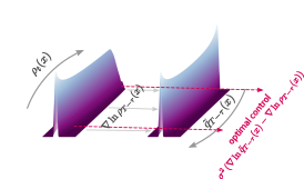
Figure 1: Schematic of the proposed control framework.

For flows without path costs $\left(U(x,t)\equiv 0\right)$, we express the particle dynamics as a system of ordinary differential equations (ODEs) [30]

$$dX^{(i)}_{t}=f(X^{(i)}_{t},t)\,dt-\nicefrac{{\sigma^{2}}}{{2}}\hat{\nabla}\ln\hat{\rho}_{t}(X^{(i)}_{t})\,dt,$$ (12)

where $\hat{\nabla}\ln\hat{\rho}_{t}(X^{(i)}_{t})$ denotes the estimated score function of the empirical distribution $\hat{\rho}_{t}(x)$.

For flows with path costs $\left(U(x,t)\neq 0\right)$, the flow dynamics in terms of operator exponentials reads

$$\rho_{t+\delta t}(x) =e^{\delta t({\cal{L}}_{f}-U(x,t))}\rho_{t}(x)$$ (13)

$$=e^{-\delta tU(x,t)}e^{\delta t{\cal{L}}_{f}}\rho_{t}(x)+\mathcal{O}((\delta t)^{2}).$$

We interpret Eq.(13) as the concatenation of two processes: a density propagation by the uncontrolled Fokker–Planck equation, followed by a multiplication by a factor $e^{-\delta tU(x,t)}$. To simulate this two-stage process for a time interval $\delta t$, we first evolve the particles following Eq.(12) to auxiliary positions $Y^{(i)}_{t}$ and assign to each particle $i$ a weight $\Omega_{i}(t)\propto e^{-\delta tU(Y^{(i)}_{t},t)}.$ To transform the weighted particles to unweighted ones, we employ the ensemble transform particle filter [31]. This method provides an optimal transport map that deterministically transforms an ensemble of weighted particles into an ensemble of uniformly weighted ones by maximising the covariance between the two ensembles.

Sparse kernel score function estimator.

To estimate the scores of the flows $\rho_{t}(x)$ and $\tilde{q}_{t}(x)$ for the particle evolution (Eq.(12)) and the estimation of optimal controls $u^{*}(x,t)$, we employ a sparse kernel score function estimator [30]. More precisely, we obtain each dimensional component $a\in[1,\dots,d]$ of $\nabla\ln\rho(x)$ from the solution of the variational problem of minimising the functional $\mathcal{I}_{\alpha}[h,\rho]$

$$\vspace{-0pt}{\partial_{\alpha}}\ln\rho(x)=\arg\min_{h}\;{\cal{I}}_{\alpha}[h,\rho]{(x)}=\arg\min_{h}\;\int\rho(x)\left(2\partial_{\alpha}h(x)+h^{2}(x)\right)dx.$$ (14)

To regularise this optimisation we assume that $h$ belongs to a Reproducing Kernel Hilbert Space associated with a radial basis function kernel, and employ a sparse kernel approximation by expressing $h$ as a linear combination of the kernel evaluated at $M\ll N$ inducing points $Z_{i}$, $h(x)=\sum_{i=1}^{M}b_{i}K(Z_{i},x)$. (See AppendixA.1 for the exact formulation of the estimator.)

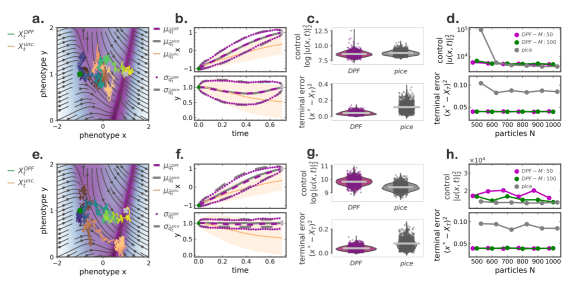
Figure 2: Deterministic particle flow (DPF) control provides optimal interventions to drive the system to target state (grey cross). (a.) Example controlled trajectory (blue-yellow) successfully reaches target, while an uncontrolled one (orange) remains in the vicinity of initial state for the same time interval. (b.) Agreement between summary statistics of marginal densities estimated from $1000$ trajectories controlled by DPF (purple) and PICE (grey) (transient mean $\mu_{\hat{q}_{t}}$ and standard deviation $\sigma_{\hat{q}_{t}}$). Orange indicates mean and standard deviation of $1000$ uncontrolled trajectories. (Used $N=400$ particles for DPF, and $N=500$ for PICE to obtain the optimal controls.) (c.) Comparison of (upper) (logarithmic) control energy, and (lower) deviation of terminal state from target for each controlled trajectory (dots) with interventions computed according to DPF (magenta) and PICE (grey). Light grey lines identify the mean of each quantity over the $1000$ trajectories. (d.)(upper) Control energy, and (lower) terminal error for increasing particle number $N$. (inducing point number for DPF magenta: $M=50$, green: $M=100$ ). Grey line indicates the performance of PICE in the same setting. (e.-h.) Same as (a.-d.) with additional path constraint $U((x,y),t)=10^{3}(y-1)^{2}$.

3 Numerical Experiments

We employed our method (deterministic particle flow control-DPF) on a model that can be thought of as describing the mean phenotype $(x,y)$ of a population evolving on a phenotypic landscape $F$ under adaptive pressures $f([x,y],t)=\nabla F(x,y)=\nabla((1-x)^{2}+(y-x^{2})^{2})$ and genetic drift represented by white noise [7].(See Appendix for more biological relevance.)

Starting from initial state $\textbf{x}_{0}=(-1,1)$, we evaluate our framework on two scenarios: one with only terminal constraints $\chi(\mathbf{x})=\delta(\mathbf{x}-\mathbf{x}^{*})$, with $\mathbf{x}^{*}=(1,1)$ (Figure 2(a.-d.)), and one with the same terminal constraints coupled with a path cost that limits fluctuations along the $y$ axis (Figure 2(e.-h.)). In both settings, we benchmark our method against the path integral cross entropy method (PICE) [24], by comparing summary statistics, control costs $\|u(\mathbf{x},t)\|^{2}_{2}$, and deviations from target $\|X_{T}-\mathbf{x}^{*}\|^{2}$ of $1000$ independent trajectories controlled by each framework (purple:DPF, grey:PICE).

Our method successfully controlled the system towards the predefined target ($\mathbf{x}^{*}$-grey cross) (Figure 2 a.,e.), and showed complete agreement with PICE in terms of the transient mean and standard deviation of the marginal densities $q_{t}(x)$ captured by the $1000$ trajectories controlled with each method. Comparing the control effort characterising the optimality of the interventions (Figure 2 c.,g.), both methods dissipated comparable energy with DPF showing slightly larger variance among individual trajectories. Nevertheless, by examining the terminal errors, DPF was consistently more accurate and precise in reaching the target. Comparing the performance of both methods for increasing particle number employed for obtaining the controls, our approach delivered more efficient controlled from PICE for small number of particles ($N=500$), while both methods were comparable for increasing particle number (Figure 2 d.). These results suggest that our method delivers equally optimal controls with PICE in one-shot, while it is also relatively more accurate in reaching the targets.

4 Conclusions

Forward-backward algorithms for smoothing densities have been extensively used in hidden Markov models. Here by relying on the duality between inference and control [32, 19, 33, 34], we borrowed ideas from the inference literature to derive non-iterative sampling schemes for constraining diffusive systems. By employing score function estimation, and recent deterministic approaches for solving Fokker–Planck equations, we proposed a non-iterative stochastic control framework that relies solely on deterministic particle dynamics. Our method interpolates between classical space-discretising PDE solutions that are inherently non-iterative, and stochastic Monte Carlo ’particle’ methods that rely on the Feynaman-Kac formula to obtain PDE solutions through sample paths.

The major limitation in applying our approach more broadly in higher dimensional systems is the curse of dimensionality. The number of particles required to provide enough evidence for accurate score estimation increases with system dimension, and more advanced methods of model reduction shall be combined with the present work. A further computational bottleneck when path constraints are pertinent is the computational complexity of ensemble transform particle filter algorithm ($\mathcal{O}(N^{3}\log N)$ [35]).Yet, there is room for improvement here by applying entropy regularised approaches for particle reweighting [36].

Appendix A Appendix

A.1 Score function estimator

The empirical formulation of the score estimator from $N$ particles representing an unknown density $\rho(x)$ is

$${\partial_{\alpha}}\ln\rho(x)\approx\sum_{i=1}^{M}\left(\sum^{M}_{k=1}B_{ik}(x)\sum^{N}_{l=1}\nabla_{X_{l}}K(X_{l},Z_{k})\right),$$ (15)

with $B_{ik}$ denoting the $i$-th row, and $k$-th column of the matrix $B(x)$ defined as

$$B(x)\doteq K(x,\mathcal{Z})\left[\lambda I+(K(\mathcal{Z},\mathcal{Z}))^{-1}(K(\mathcal{X},\mathcal{Z}))^{\top}(K(\mathcal{X},\mathcal{Z}))\right]^{-1}(K(\mathcal{Z},\mathcal{Z}))^{-1},$$ (16)

where $\mathcal{X}=\{X_{i}\}^{N}_{i=1}$ and $\mathcal{Z}=\{Z_{i}\}^{M}_{i=1}$ denote the sets of samples and inducing points respectively, while $I$ stands for an $M\times M$ identity matrix. (Here we set the regularising constant $\lambda=10^{-3}$). We used an gaussian kernel

$$K(x,x^{\prime})=\exp\left[-\frac{1}{2{l}^{2}}\|x-x^{\prime}\|^{2}\right],$$ (17)

where the lengthscale $l$ was set to two times the standard deviation of the particle ensemble for each time step.

A.2 Implementation details

Here we provide the algorithm for computing optimal interventions $u^{*}(x,t)$. Since the initial conditions for the flows $\rho_{t}(x)$ and $\tilde{q}_{t}(x)$ are delta functions centered around the initial and target state, $x_{0}$ and $x_{1}$, i.e $\rho_{0}(x)=\delta(x-x_{0})$ and $\tilde{q}_{t}(x)=\delta(x-x_{1})$, we employ a single stochastic step at the beginning of each (forward and time-reversed) flow propagation. Since the inducing point number $M$ employed in the gradient–log–density estimation is considerably smaller than sample number $N$, i.e., $M\ll N$, the overall computational complexity of a single gradient-log-density evaluation amounts to $\mathcal{O}\left(N\,M^{2}\right)$. We perform Euler integration for the ODEs, and Euler-Maruyama for stochastic simulations. For all numerical integrations we employ $dt=10^{-3}$ discretisation step. For the numerical experiments with path constraints, we solved the optimal transport problem with the implementation of FastEMD [37].

For some of the visualisations of our results we used the Seaborn [38] python toolbox.

References

- [1] Carsten Hartmann and Christof Schütte. Efficient rare event simulation by optimal nonequilibrium forcing. Journal of Statistical Mechanics: Theory and Experiment, 2012(11):P11004, 2012.
- [2] Raphaël Chetrite and Hugo Touchette. Variational and optimal control representations of conditioned and driven processes. Journal of Statistical Mechanics: Theory and Experiment, 2015(12):P12001, 2015.
- [3] Jin Won Kim and Prashant G Mehta. An optimal control derivation of nonlinear smoothing equations. In Proceedings of the Workshop on Dynamics, Optimization and Computation held in honor of the 60th birthday of Michael Dellnitz, pages 295–311. Springer, 2020.
- [4] Emanuel Todorov. Efficient computation of optimal actions. Proceedings of the National Academy of Sciences of the United States of America, 106(28):11478–11483, 2009.
- [5] Hilbert J Kappen. Linear theory for control of nonlinear stochastic systems. Physical Review Letters, 95(20):200201, 2005.
- [6] Daniel K Wells, William L Kath, and Adilson E Motter. Control of stochastic and induced switching in biophysical networks. Physical Review X, 5(3):031036, 2015.
- [7] Armita Nourmohammad and Ceyhun Eksin. Optimal evolutionary control for artificial selection on molecular phenotypes. Physical Review X, 11(1):011044, 2021.
- [8] Ziwei Zhong, Brandon G Wong, Arjun Ravikumar, Garri A Arzumanyan, Ahmad S Khalil, and Chang C Liu. Automated continuous evolution of proteins in-vivo. ACS synthetic biology, 9(6):1270–1276, 2020.
- [9] Ta-Chu Kao, Mahdieh S Sadabadi, and Guillaume Hennequin. Optimal anticipatory control as a theory of motor preparation: a thalamo-cortical circuit model. Neuron, 109(9):1567–1581, 2021.
- [10] Alexandre Iolov, Susanne Ditlevsen, and André Longtin. Stochastic optimal control of single neuron spike trains. Journal of Neural Engineering, 11(4):046004, 2014.
- [11] Stephen H Scott. Optimal feedback control and the neural basis of volitional motor control. Nature Reviews Neuroscience, 5(7):532–545, 2004.
- [12] Espen Bernton, Jeremy Heng, Arnaud Doucet, and Pierre E Jacob. Schrödinger Bridge Samplers. arXiv preprint arXiv:1912.13170, 2019.
- [13] Francisco Vargas, Pierre Thodoroff, Neil D Lawrence, and Austen Lamacraft. Solving Schrödinger Bridges via Maximum Likelihood. arXiv preprint arXiv:2106.02081, 2021.
- [14] Ioannis Exarchos and Evangelos A Theodorou. Stochastic optimal control via forward and backward stochastic differential equations and importance sampling. Automatica, 87:159–165, 2018.
- [15] Yang Song, Jascha Sohl-Dickstein, Diederik P Kingma, Abhishek Kumar, Stefano Ermon, and Ben Poole. Score-based generative modeling through stochastic differential equations. arXiv preprint arXiv:2011.13456, 2020.
- [16] Igor Vladimirovich Girsanov. On transforming a certain class of stochastic processes by absolutely continuous substitution of measures. Theory of Probability and Its Applications, 5(3):285–301, 1960.
- [17] Bernt Øksendal. Stochastic differential equations. Springer, 2003.
- [18] Evangelos A Theodorou and Emanuel Todorov. Relative entropy and free energy dualities: Connections to path integral and kl control. In 2012 IEEE 51st IEEE Conference on Decision and Control (cdc), pages 1466–1473. IEEE, 2012.
- [19] Hilbert J Kappen, Vicenç Gómez, and Manfred Opper. Optimal control as a graphical model inference problem. Machine Learning, 87(2):159–182, 2012.
- [20] Richard Bellman. Dynamic programming and Lagrange multipliers. Proceedings of the National Academy of Sciences of the United States of America, 42(10):767, 1956.
- [21] Wendell H Fleming. Exit probabilities and optimal stochastic control. Applied Mathematics and Optimization, 4(1):329–346, 1977.
- [22] Jochen Garcke and Axel Kröner. Suboptimal feedback control of PDEs by solving HJB equations on adaptive sparse grids. Journal of Scientific Computing, 70(1):1–28, 2017.
- [23] Mario Annunziato and Alfio Borzì. A Fokker–Planck control framework for multidimensional stochastic processes. Journal of Computational and Applied Mathematics, 237(1):487–507, 2013.
- [24] Hilbert Johan Kappen and Hans Christian Ruiz. Adaptive importance sampling for control and inference. Journal of Statistical Physics, 162(5):1244–1266, 2016.
- [25] Wei Zhang, Han Wang, Carsten Hartmann, Marcus Weber, and Christof Schuette. Applications of the cross-entropy method to importance sampling and optimal control of diffusions. SIAM Journal on Scientific Computing, 36(6):A2654–A2672, 2014.
- [26] Nicolas Macris and Raffaele Marino. Solving non-linear Kolmogorov equations in large dimensions by using deep learning: a numerical comparison of discretization schemes. arXiv preprint arXiv:2012.07747, 2020.
- [27] Zongyi Li, Nikola Kovachki, Kamyar Azizzadenesheli, Burigede Liu, Kaushik Bhattacharya, Andrew Stuart, and Anima Anandkumar. Fourier neural operator for parametric partial differential equations. International Conference on Learning Representations, 2020.
- [28] Yariv Ephraim and Neri Merhav. Hidden markov processes. IEEE Transactions on Information Theory, 48(6):1518–1569, 2002.
- [29] Leonard E Baum, Ted Petrie, George Soules, and Norman Weiss. A maximization technique occurring in the statistical analysis of probabilistic functions of Markov chains. The Annals of Mathematical Statistics, 41(1):164–171, 1970.
- [30] Dimitra Maoutsa, Sebastian Reich, and Manfred Opper. Interacting particle solutions of Fokker–Planck equations through gradient–log–density estimation. Entropy, 22(8):802, 2020.
- [31] Sebastian Reich. A nonparametric ensemble transform method for Bayesian inference. SIAM Journal on Scientific Computing, 35(4):A2013–A2024, 2013.
- [32] Emanuel Todorov. General duality between optimal control and estimation. In 2008 47th IEEE Conference on Decision and Control, pages 4286–4292. IEEE, 2008.
- [33] Sergey Levine. Reinforcement learning and control as probabilistic inference: Tutorial and review. arXiv preprint arXiv:1805.00909, 2018.
- [34] Hagai Attias. Planning by probabilistic inference. In International Workshop on Artificial Intelligence and Statistics, pages 9–16. PMLR, 2003.
- [35] Dimitris Bertsimas and John N Tsitsiklis. Introduction to linear optimization, volume 6. Athena Scientific Belmont, MA, 1997.
- [36] Adrien Corenflos, James Thornton, George Deligiannidis, and Arnaud Doucet. Differentiable particle filtering via entropy-regularized optimal transport. In International Conference on Machine Learning, pages 2100–2111. PMLR, 2021.
- [37] Ofir Pele and Michael Werman. Fast and robust earth mover’s distances. In 2009 IEEE 12th International Conference on Computer Vision, pages 460–467. IEEE, September 2009.
- [38] Michael L Waskom. Seaborn: statistical data visualization. Journal of Open Source Software, 6(60):3021, 2021.