Logsig-RNN: a novel network for robust and efficient skeleton-based action recognition

Abstract

This paper contributes to the challenge of skeleton-based human action recognition in videos. The key step is to develop a generic network architecture to extract discriminative features for the spatio-temporal skeleton data. In this paper, we propose a novel module, namely Logsig-RNN, which is the combination of the log-signature layer and recurrent type neural networks (RNNs). The former one comes from the mathematically principled technology of signatures and log-signatures as representations for streamed data, which can manage high sample rate streams, non-uniform sampling and time series of variable length. It serves as an enhancement of the recurrent layer, which can be conveniently plugged into neural networks. Besides we propose two path transformation layers to significantly reduce path dimension while retaining the essential information fed into the Logsig-RNN module. (The network architecture is illustrated in Figure 1 (Right).) Finally, numerical results demonstrate that replacing the RNN module by the Logsig-RNN module in SOTA networks consistently improves the performance on both Chalearn gesture data and NTU RGB+D 120 action data in terms of accuracy and robustness. In particular, we achieve the state-of-the-art accuracy on Chalearn2013 gesture data by combining simple path transformation layers with the Logsig-RNN. Codes are available at https://github.com/steveliao93/GCN_LogsigRNN.

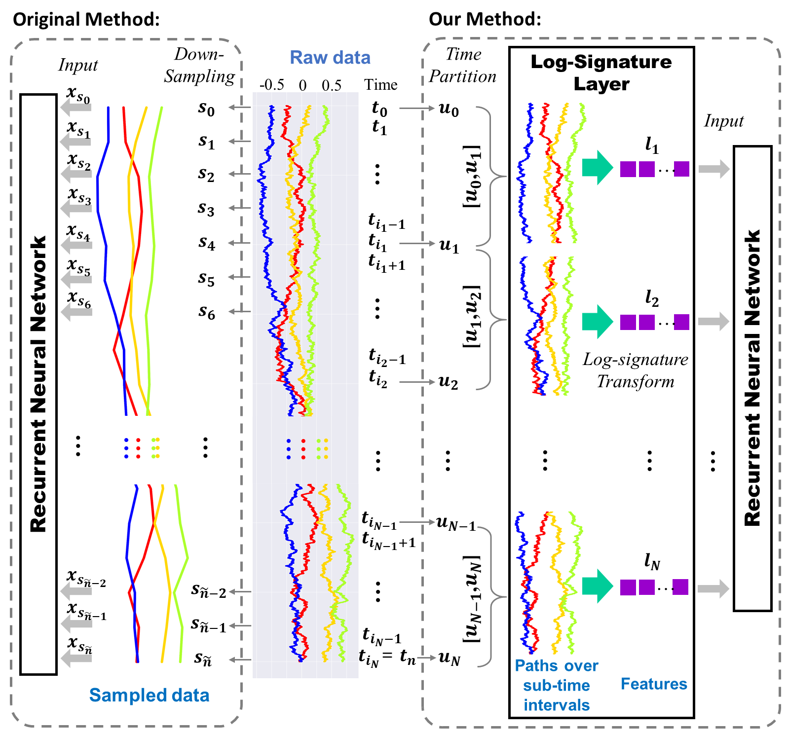
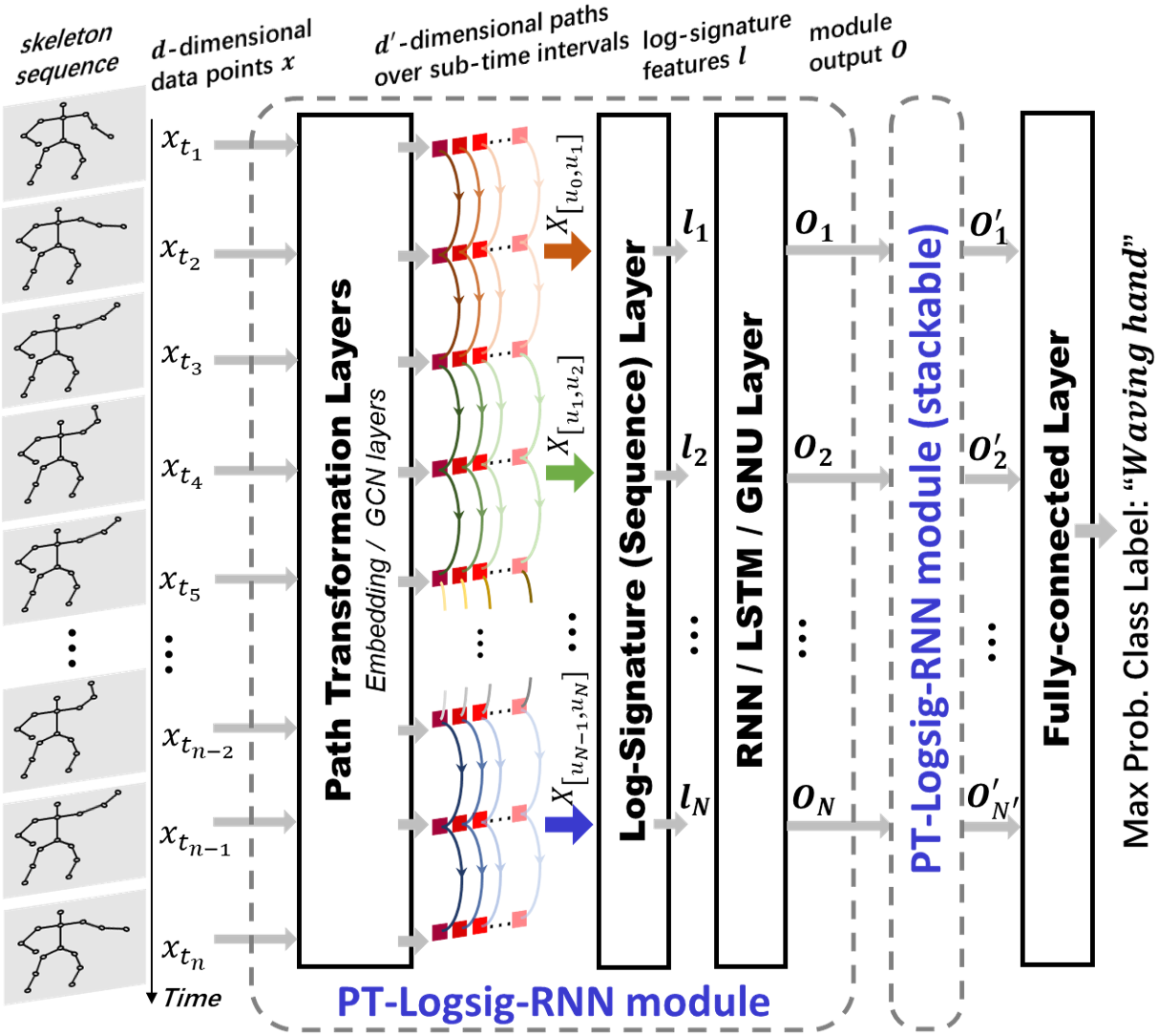
Figure 1: (Left) Comparison of Logsig-RNN and RNN; (Right) Pipeline of the PT-Logsig-RNN module for skeleton-based human action recognition. This stackable module consists of Path Transformation Layers, followed by the Log-Signature Layer and an RNN-type layer.

Keywords Skeleton-based action recognition  $\cdot$ Recurrent neural network  $\cdot$ Deep learning  $\cdot$ Log-signature  $\cdot$ Rough path theory

1 Introduction

Human action recognition (HAR) in videos is a classical and challenging problem in computer vision with a wide range of applications in human-computer interfaces and communications. Low-cost motion sensing devices, e.g. Microsoft Kinect, and reliable pose estimation methods, are both leading to an increase in popularity of research and development on skeleton-based HAR (SHAR). Compared with RGB-D HAR, skeleton-based methods are robust to illumination changes and have benefits of data privacy and security.

Although vast literature is devoted to SHAR Lo Presti and La Cascia (2016); Wang et al. (2019a); Ren et al. (2020), the challenge remains open due to two main issues: (1) how to extract discriminative representations for the high dimensional spatial structure of skeletons; (2) how to model the temporal dynamics of motion.

With the increasing development and impressive performance of deep learning models e.g. Recurrent Neural Networks (RNN) Lev et al. (2016); Liu et al. (2016, 2018); Shahroudy et al. (2016); Wang and Wang (2017), Convolutional Neural Networks (CNN) Caetano et al. (2019); Chéron et al. (2015); Ke et al. (2018); Li et al. (2018); Liu et al. (2019a); Liu and Yuan (2018), and Graph Convolutional Networks (GCN) Li et al. (2019a); Shi et al. (2019), data-driven deep features have gained increasing attention in SHAR Ren et al. (2020). However, these methods are often data greedy and computationally expensive, and not well adapted to data of different sizes/lengths. For example, when the lengths of data sequences are long and diverse, long-short term memory networks (LSTMs) either suffer from tremendous training cost with heuristic padding or are forced to down-sample/re-sample the data, which potentially misses the microscopic information.

To address some of the difficulties and better capture the temporal dynamics, we propose a simple but effective neural network module, namely Logsig-RNN, by blending the Log-signature (Sequence) Layer with the RNN layer, as shown in Figure 1 (Left). The log-signature, which was originally introduced in rough path theory in the field of stochastic analysis, is an effective mathematical tool to summarize and vectorize complex un-parameterized streams of multi-modal data over a coarse time scale with a low dimensional representation, reducing the number of timesteps in the RNN. The properties of the log-signature also allow to handle time series with variable length without the use of padding and provide robustness to missing data. This allows the following RNN layer to learn more expressive deep features, leading to a systematic method to treat the complex time series data in SHAR.

The spatial structure in SHAR methods is commonly modelled using coordinates of joints Fan et al. (2016); Jhuang et al. (2013); Yang and Tian (2014), using body parts to model the articulated system Evangelidis et al. (2014); Li and Leung (2016); Shahroudy et al. (2015) or by hybrid methods using information from both joints and body parts Ke et al. (2017); Li et al. (2018). Inspired by Li et al. (2018) and Liu et al. (2020), we investigate combining the flexible Logsig-RNN with Path Transformation Layers (PT) which include an Embedding Layer (EL) to reduce the spatial dimension of pure joint information and a vanilla Graph Convolutional Layer (GCN) to learn to implicitly capture the discriminative joints and body parts.

Our pipeline for SHAR is illustrated in Figure 1 (Right). With quantitative analysis on Chalearn2013 gesture dataset and NTU RGB+D 120 action dataset, we validated the efficiency and robustness of Logsig-RNN and the effects of the Path Transformation layers.

2 Related Works on Signature Feature

The signature feature (SF) of a path, originated from rough path theory Lyons (1998), was introduced as universal feature for time-series modelling Levin et al. (2013) and has been successfully applied to machine learning (ML) tasks, e.g. financial data analysis Gyurkó et al. (2013); Lyons et al. (2014), handwriting recognition Diehl (2013); Graham (2013); Yang et al. (2016a); Xie et al. (2018), writer identification Yang et al. (2016b), signature verification Lai et al. (2017), psychiatric analysis Arribas et al. (2018), speech emotion recognition Wang et al. (2019b) as well as action classification Ahmad et al. (2019); Király and Oberhauser (2016); Li et al. (2019b); Yang et al. (2017). These SF-based methods can be grouped into the whole-interval manner and sliding-window manner. The whole-interval manner regards data streams of various lengths as paths over the entire time interval; then the SFs of fixed dimensions are computed to encode both global and local temporal dependencies Levin et al. (2013); Diehl (2013); Lai et al. (2017); Arribas et al. (2018); Wang et al. (2019b); Yang et al. (2017); Li et al. (2019b). The sliding-window manner computes the SFs over window-based sub-intervals which are viewed as local descriptors and are further aggregated by deep networks Graham (2013); Yang et al. (2016a, b); Xie et al. (2018); Li et al. (2017). Our method falls into the second category using disjoint sliding windows. There are few works on using the log-signature, rather than the signature, in ML applications Li et al. (2017); Kidger et al. (2021). In this paper, we demonstrate the properties, efficiency, and robustness of the log-signature compared with the signature. Recent work Kidger et al. (2019) proposed to use the signature transformation as a layer rather than as a feature extractor. We propose a Log-signature (Sequence) Layer with impressive advantages in temporal modelling to improve RNNs. To our best knowledge, it is the first of the kind to (1) integrate the log-signature sequence with RNNs (2) as a differentiable layer which can be used anywhere within a larger model, instead of using the log signature as feature extractor. In particular, the output of the LogsigRNN is of the same shape as its input with a reduced time dimension.

3 The Log-Signature of a Path

Let $E:=\mathbb{R}^{d}$, $J=[S,T]$ and $X:J\rightarrow E$ be a continuous path endowed with a norm denoted by $|\cdot|$. In practice we may only observe $X$ built at some fine scale out of time stamped values $X^{\hat{\mathcal{D}}}=[X_{t_{1}},X_{t_{2}},\cdots,X_{t_{n}}]$, where $\hat{\mathcal{D}}=(t_{1},\cdots,t_{n})$. Throughout this paper, we embed the discrete time series $X^{\hat{\mathcal{D}}}$ to a continuous path of bounded variation by linear interpolation for a unified treatment (See detailed discussion in Section 4 of Levin et al. (2013)). Therefore, we focus on paths of bounded variation. In this section, we introduce the definition of the signature/log-signature. Then we summarize the key properties of the log-signature, which make it an effective, compact and high order feature of streamed data over time intervals. Lastly, we highlight the comparison between the log-signature and the signature. Further discussions and demo codes on the (log)-signature can be found in the supplementary material.

3.1 The (log)-signature of a path

The background information and practical calculation of the signature as a faithful feature set for un-parameterized paths can be found in Kidger et al. (2019); Levin et al. (2013); Chevyrev and Kormilitzin (2016). We introduce the formal definition of the signature in this subsection.

Definition 3.1 (Total variation).

The total variation of a continuous path $X:J\to E$ is defined on the interval $J$ to be $||X||_{J}=\sup_{\mathcal{D}\subset J}\sum_{j=0}^{r-1}\left|X_{t_{j+1}}-X_{t_{j}}\right|$, where the supremum is taken over any time partition of $J$, i.e. $\mathcal{D}=(t_{1},t_{2},\cdots,t_{r})$.

Any continuous path $X:J\to E$ with finite total variation, i.e. $||X||_{J}<\infty$, is called a path of bounded variation. Let $BV(J,E)$ denote the range of any continuous path mapping from $J$ to $E$ of bounded variation.

Let $T((E))$ denote the tensor algebra space endowed with the tensor multiplication and componentwise addition, in which the signature and the log signature of a path take values.

Definition 3.2 (The Signature of a Path).

Let $X\in BV(J,E)$. Define the $k^{th}$ level of the signature of the path $X_{J}$ as $\mathbf{X}^{k}_{J}=\int_{S}^{T}\dots\int_{S}^{u_{2}}dX_{u_{1}}\otimes\dots\otimes dX_{u_{n}}.$ The signature of $X$ is defined as $S(X_{J})=(1,\mathbf{X}_{J}^{1},\dots,\mathbf{X}_{J}^{k},\dots)$. Let $S_{k}(X_{J})$ denote the truncated signature of $X$ of degree $k$, i.e. $S_{k}(X_{J})=(1,\mathbf{X}_{J}^{1},\dots,\mathbf{X}_{J}^{k}).$

Then we proceed to define the logarithm map in $T((E))$ in terms of a tensor power series as a generalization of the scalar logarithm.

Definition 3.3 (Logarithm map).

Let $a=(a_{0},a_{1},\cdots)\in T((E))$ be such that $a_{0}=1$ and $t=a-1$. Then the logarithm map denoted by $\log$ is defined as follows:

$$\log(a)=\log(1+t)=\sum_{n=1}^{\infty}\frac{(-1)^{n-1}}{n}t^{\otimes n},\forall a\in T((E)).$$ (1)

Definition 3.4 (The Log Signature of a Path).

For $X\in BV(J,E)$, the log signature of a path $X$ denoted by $lS(X_{J})$ is the logarithm of the signature of the path $X$. Let $lS_{k}(X_{J})$ denote the truncated log signature of a path $X$ of degree $k$.

The first level of the log-signature of a path $X$ is the increment of the path $X_{T}-X_{S}$. The second level of the log-signature is the signed area enclosed by $X$ and the chord connecting the end and start of the path $X$. There are three open-source python packages esig Lyons et al. , iisignature Jeremy and Benjamin. (2018) and signatory Kidger and Lyons (2020) to compute the log-signature.

3.2 Properties of the log-signature

Uniqueness: By the uniqueness of the signature and bijection between the signature and log-signature, it is proved that the log-signature determines a path up to tree-like equivalence Hambly and Lyons (2010). The log-signature encodes the order information of a path in a graded structure. Note that adding a monotone dimension, like the time, to a path can avoid tree-like sections.
Invariance under time parameterization: We say that a path $\tilde{X}:J\rightarrow E$ is the time re-parameterization of $X:J\rightarrow E$ if and only if there exists a non-decreasing surjection $\lambda:J\rightarrow J$ such that $\tilde{X}_{t}=X_{\lambda(t)}$, $\forall t\in J$. Let $X\in BV(J,E)$ and a path $\tilde{X}:J\rightarrow E$ be a time re-parameterization of $X$. Then it is proved that the log-signatures of $X$ and $\tilde{X}$ are equalLyons (1998). This is illustrated in figure 2, where speed changes result in different time series representation but the same log-signature feature. This is beneficial as human motions are invariant under the change of video frame rates. The log-signature feature can remove the redundancy caused by the speed of traversing the path, which brings massive dimensionality reduction.

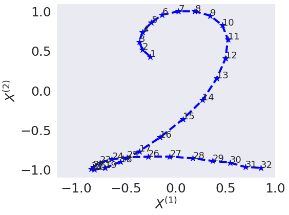
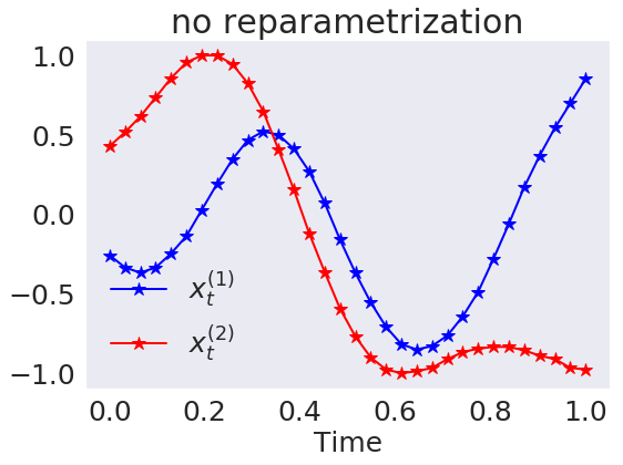
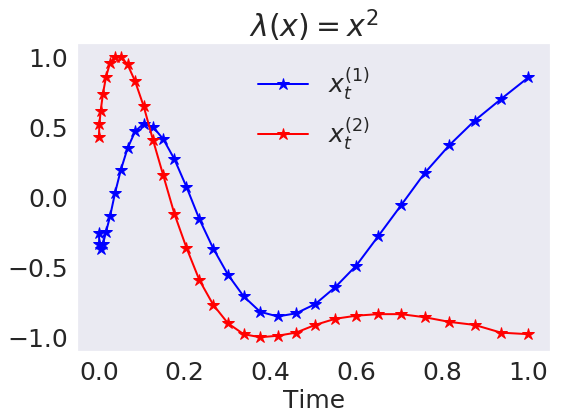
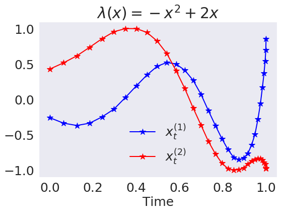
Figure 2: The first figure represents the trajectory of the digit $2$, and the rest of figures plot the coordinates of the pen locations against time via different speed respectively, which share the same signature and log signature given in the first subplot.

 
Irregular time series: The truncated log-signature feature provides a robust descriptor of fixed dimension for time series of variable length, uneven time spacing and with missing data. For example, given a pen digit trajectory, random sub-sampling results in new trajectories of variable length and non-uniform spacing. In this case, the mean absolute percentage error (MAPE) of the log-signature is small (see Figure 3 in supplementary material).

3.3 Comparison between signature and log-signature

The logarithm map is bijective on the domain $\{a\in T((E))|a_{0}=1\}$. Thus the log-signature and the signature is one-to-one. Therefore, the signature and log-signature share all the properties covered in the previous subsection. In the following, we highlight important differences between the signature and the log-signature.

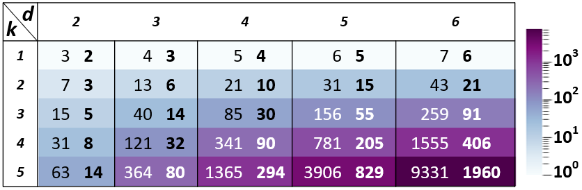
Figure 3: The dimension comparison between the signature and log-signature (in bold) of a $d$-dimensional path of degree $k$.

The log-signature is a parsimonious representation for the signature feature, whose dimension is lower than that of the signature in general. For $d>2$, the dimension of the signature of a $d$-dimension path up to degree $k$ is $\frac{d^{k+1}-1}{d-1}$, and the dimension of the corresponding log-signature is equal to the necklace polynomial on $(d,k)$Reizenstein and Graham (2018). Figure 3 shows that the larger $d$ and $k$, the greater dimension reduction the log-signature brings over the signature (the colour represents the dimension gap between signature and the log signature). In contrast to the signature, the log-signature does not have universality, and thus it needs to be combined with non-linear models for learning.

4 PT-Logsig-RNN Network

In this section, we propose a simple, compact and efficient PT-Logsig-RNN Network for SHAR, which is composed of (1) path transformation layers, (2) the Logsig-RNN module and (3) a fully connected layer. The overall PT-Logsig-RNN model is depicted in Figure 1 (Right). We start by introducing the Log-Signature Layer and follow with the core module of our model, the Logsig-RNN module. In the end, we propose useful path transformation layers to further improve the performance of the Logsig-RNN module in SHAR tasks.

4.1 Log-Signature Layer

We propose the Log-Signature (Sequence) Layer, which transforms an input data stream to a sequence of log-signatures over sub-time intervals. More specifically, consider a $d$-dimensional stream $x\in BV(J,E)$ and let $\mathcal{D}:=(u_{k})_{k=0}^{N}$ be a time partition of $J$.

Definition 4.1 (Log-Signature (Sequence) Layer).

A Log-Signature Layer of degree $M$ associated with $\mathcal{D}$ is a mapping from $BV(J,E)$ to $\mathbb{R}^{N\times d_{ls}}$ such that $\forall x\in BV(J,E)$, $x\mapsto(l_{k}^{M})_{k=0}^{N-1}$, where $l_{k}^{M}$ is the truncated log signature of $x_{[u_{k},u_{k+1}]}$ of degree $M$, i.e. $l_{k}^{M}=lS_{M}(x_{[u_{k},u_{k+1}]})$. Here $d_{ls}$ is the dimension of the log-signature of a $d$-dimensional path of degree $M$.

In practice, the input stream $x$ is usually only observed at a finite collection of time points $\hat{\mathcal{D}}$, which can be non-uniform, high frequency and sample-dependent. By interpolation, embedding $x^{\hat{\mathcal{D}}}$ to the path space allows the Log-Signature Layer to treat each sample stream over $\mathcal{D}$ in a unified way. The output dimension of the Log-Signature Layer is $(N,d_{ls})$, which does not depend on the time dimension of the input streams. A higher frequency of input data would not cause any dimension issue, but it makes the computation of $l_{k}$ more accurate. The Log-Signature Layer can shrink the time dimension of the input stream effectively, while preserving local temporal information by using the log-signatures.

It is noted that the Log-Signature Layer does not have any trainable parameters, but allows backpropagation through it. We extend the work on the backpropagation algorithm of single log-signatures in Reizenstein and Graham (2018) to log-signature sequences. Our implementation can accommodate time series samples of variable length over sub-time intervals, which may not be directly handled by the Log-Signature layer in the signatory packageKidger and Lyons (2020).

4.2 Logsig-RNN Network

Firstly, we introduce the conventional recurrent neural network. It is composed of three types of layers, i.e. the input layer $(x_{t})_{t}$, the hidden layer $(h_{t})_{t}$ and the output layer $(o_{t})_{t}$. A RNN takes an input sequence $x^{\hat{\mathcal{D}}}=(x_{t_{i}})_{i=1}^{T}$ and computes an output $(o_{t})_{t=1}^{T}\in\mathbb{R}^{T\times e}$ via $h_{t}=\sigma(Ux_{t}+Wh_{t-1}),o_{t}=q(Vh_{t})$, where $U$, $W$ and $V$ are model parameters, and $\sigma$ and $q$ are activation functions. Let $\mathcal{R}_{\Theta}((x_{t})_{t})$ denote the RNN model with $(x_{t})_{t}$ as the input and $\Theta:=\{U,W,V\}$ its parameter set. It is noted that this represents all the recurrent type neural networks, including LSTM, GRU, etc. Then we propose the following Logsig-RNN model.

Model 4.1 (Logsig-RNN Network).

Given $\mathcal{D}:=(u_{k})_{k=0}^{N}$, a Logsig-RNN network computes a mapping from an input path $x\in BV(J,E)$ to an output defined as follows:

• Compute $(l_{k})_{k=0}^{N-1}$ as the output of the Log-Signature Layer of degree $M$ associated with $\mathcal{D}$ for an input $x$.

• The output layer is computed by $\mathcal{R}_{\Theta}((l_{k})_{k=0}^{N-1})$, where $\mathcal{R}_{\Theta}$ is a RNN type network.

The Logsig-RNN model (depicted in Figure 1 (Left)) is a natural generalization of conventional RNNs. When $\mathcal{D}$ coincides with timestamps of the input data, the Logsig-RNN Model with $M=1$ is the RNN model with the increments of the data as input. One main advantage of our method is to reduce the time dimension of the RNN model significantly as we use the principled, non-linear and compact log-signature features to summarize the data stream locally. It leads to higher accuracy and efficiency compared with the standard RNN model. Logsig-RNN can overcome the limitation of Sig-OLR Levin et al. (2013) on stability and efficiency issues by using compact log-signature features and more effective non-linear RNN models. Compared with conventional RNNs the Logsig-RNN model has the same input and output structure.

4.3 Path Transformation Layers

To more efficiently and effectively exploit the spatio-temporal structure of the path, we further investigate the use of two main path transformation layers (i.e. Embedding Layer and Graph Convolutional Layer) in conjunction with the Log-Signature Layer.

A skeleton sequence $X$ can be represented as a $n\times F\times D$ tensor (landmark sequence) and a $F\times F$ matrix $\mathcal{A}$ (bone information), where $n$ is the number of frames in the sequence, $F$ is the number of joints in the skeleton, $D$ is the coordinate dimension and $\mathcal{A}$ is the adjacency matrix to denote whether two joints have a bone connection or not.

Embedding Layer (EL) In the literature, many models only use landmark data without explicit bone information. One can view a skeleton sequence as a single path of high dimension($d$) (e.g. a skeleton of 25 3D joints has $d=F\cdot D=75$). Since the dimension of the truncated log-signature grows fast w.r.t. $d$, we add a linear Embedding Layer before the Log-Signature Layer to reduce the spatial dimension and avoid this issue. Motivated by Li et al. (2018), we first apply a linear convolution with kernel dimension 1 along the time and joint dimensions to learn a joint level representation. Then we apply full convolution on the second and third coordinates to learn the interaction between different joints for an implicit representation of skeleton data. The output tensor of EL has the shape $n\times d_{el}$, where $d_{el}$ is a hyper-parameter to control spatial dimension reduction. One can view the embedding layer as a learnable path transformation that can help to increase the expressivity of the (log)-signature.

In practice, the Embedding Layer is more effective when subsequently adding the Time-Incorporated Layer (TL) and the Accumulative Layer (AL). The details of TL and AL can be found in Section 5 in the appendix. For simplicity we will use EL to denote the Embedding Layer composed with TL and AL in the below numerical experiments.

Graph Convolutional Layer (GCN) Recently, graph-based neural networks have been introduced and achieved SOTA accuracy in several SHAR tasks due to their ability to extract spatial information by incorporating additional bone information using graphs. We demonstrate how a GCN and the Logsig-RNN can be combined to form the GCN-Logsig-RNN to model spatio-temporal information.

First, we define the GCN layer on the skeleton sequence. Let $G_{\theta}$ denote a graph convolutional operator $F\times D\rightarrow F\times\tilde{D}$ associated with $\mathcal{A}$ by mapping $x$ to $(\Gamma^{-\frac{1}{2}}(\mathcal{A}+I)\Gamma^{-\frac{1}{2}})x\theta$, where $\Gamma^{ii}=\sum_{j}(\mathcal{A}^{ij}+I^{ij})$, and $I$ is the identity matrix. Then we extend $G_{\theta}$ to the skeleton sequence by applying $G_{\theta}$ to each frame $X_{t}$, i.e. $G_{\theta}:X=(X_{t})_{t=1}^{n}\mapsto(G_{\theta}(X_{t}))_{t=1}^{n}$ to obtain an output as a sequence of graphs of time dimension $n$ with the adjacency matrix $\mathcal{A}$.

Next we propose the below GCN-Logsig-RNN to combine GCN with the Logsig-RNN. Let $\hat{X}^{(i)}_{t}\in\mathbb{R}^{\tilde{D}}$ denote the features of the $i^{th}$ joint of the GCN output $G_{\theta}(X_{t})$ at time $t$. For each $i^{th}$ joint, $\hat{X}^{(i)}=(\hat{X}^{(i)}_{t})_{t=1}^{n}$ is a $\tilde{D}$-dimensional path. We apply the Logsig-RNN to $\hat{X}^{(i)}$ as the feature sequence of each $i^{th}$ joint, and hence obtain a sequence of graphs whose feature dimension is equal to the log-signature dimension and whose time dimension is the number of segments in Logsig-RNN. This in particular also allows for the module to be stacked.

5 Numerical Experiments

We evaluate the proposed EL-Logsig-LSTM model on two datasets: (1) Charlearn 2013 data, and (2) NTU RGB+D 120 data. Chalearn 2013 dataset Escalera et al. (2013) is a publicly available dataset for gesture recognition, which contains 11,116 clips of 20 Italian gestures performed by 27 subjects. Each body consists of 20 3D joints. NTU RGB+D 120 Liu et al. (2019b) is a large-scale benchmark dataset for 3D action recognition, which consists of $114,480$ RGB+D video samples that are captured from 106 distinct human subjects for 120 action classes. 3D coordinates of 50 joints in each frame are used in this paper. In our experiments, we validate the performance of our model using only the skeleton data of the above datasets.

5.1 Chalearn2013 data

State-of-the-art performance: We apply the EL-Logsig-LSTM model to Chalearn2013 and achieve state-of-the-art (SOTA) classification accuracy shown in Table 1 of the 5-fold cross validation results. The EL-Logsig-LSTM ($M=2,N=4$) with data augmentation achieves performance comparable to the SOTA Liao et al. (2019).

(a) Accuracy comparison
Methods	Accuracy(%)	Data Aug.
Deep LSTM Shahroudy et al. (2016)	87.10	$-$
Two-stream LSTM Wang and Wang (2017)	91.70	$\surd$
ST-LSTM + Trust Gate Liu et al. (2018)	92.00	$\surd$
3s_net_TTM Li et al. (2019b)	92.08	$\surd$
Multi-path CNNLiao et al. (2019)	93.13	$\surd$
LSTM0	90.92	$\times$
LSTM0 (+data aug.)	91.18	$\surd$
EL-Logsig-LSTM	91.77 $\pm$ 0.34	$\times$
EL-Logsig-LSTM(+data aug.)	92.94 $\pm$ 0.21	$\surd$
GCN-Logsig-LSTM	91.92 $\pm$ 0.28	$\times$
GCN-Logsig-LSTM(+data aug.)	92.86 $\pm$ 0.23	$\surd$

(b) Effects of EL
Methods	$D_{el}$	Accuracy(%)	# Trainable weights
With EL	10	91.09	120,594
	20	92.92	213,574
	30	93.38	357,954
	40	93.10	553,734
	50	93.33	800,914
	60	93.30	1,099,494
W/O EL	-	91.51	985,458

    (c) Effects of number of Segments ($N$) $N$ 2 4 8 Accuracy 92.10$\pm$0.04 92.94$\pm$0.21 92.69$\pm$0.11 $N$ 16 32 64 Accuracy 92.87$\pm$0.15 91.66$\pm$0.39 91.50$\pm$0.39

Table 1: The accuracy comparison and sensitivity analysis on Chalearn2013. (a) The number after $\pm$ is the standard deviation of the accuracy. (b) $D_{el}$ is the spatial dimension of EL output.

Investigation of path transformation layers: To validate the effects of EL, we compare the test accuracy and number of trainable weights in our network with and without EL on Chalearn 2013 data. Table 1 (b) shows that the addition of EL increases the accuracy by $1.87$ percentage points (pp) while reducing the number of trainable weights by over $60\%$. Let $D_{el}$ denote the spatial dimension of the output of EL. We can see that even introducing EL without a reduction in dimensionality, i.e. setting $D_{el}$ to the original spatial dimension of 60, improves the test accuracy. Decreasing the dimensionality can lead to further improvements, with the best results in our experiments at $D_{el}=30$ with a test accuracy of $93.38\%$. A further decrease of $D_{el}$ leads to the performance deteriorating. The high accuracy of our model using EL to reduce the original spatial dimension from $60$ to $D_{el}=30$ suggests that EL can learn implicit and effective spatial representations for the motion sequences. AL and TL contribute a 0.86 pp gain in test accuracy to the EL-Logsig-LSTM model.

Investigation of different segment numbers in Logsig-LSTM: Table 1 (c) shows that increasing the number of segments ($N$) up to certain threshold increases the test accuracy, and increasing $N$ further worsens the model performance. For Chalearn2013, the optimal $N$ is $4$ and the optimal network architecture is depicted in Table A.1 in the supplement material.

5.2 NTU RGB+D 120 data

For NTU 120 data, we apply the EL-Logsig-LSTM, GCN-Logsig-LSTM and a stacked two-layer GCN-Logsig-LSTM(GCN-Logsig-LSTM²) to demonstrate that the Logsig-RNN can be conveniently plugged into different neural networks and achieve competitive accuracy.

Among non-GCN models, for X-Subject protocol, our EL-Logsig-LSTM model outperforms other methods, while it is competitive with Caetano et al. (2019) and Liu and Yuan (2018) for X-Setup. The latter leverages the informative pose estimation maps as additional clues. Table 2 (Left) shows the ablation study of EL-Logsig-LSTM For the X-Subject task, adding EL layer results in a 0.7 pp gain over the baseline and the Logsig layer further gives a 5.9 pp gain.

Methods	X-Subject(%)	X-Setup(%)
ST LSTMLiu et al. (2016)	55.7	57.9
FSNetLiu et al. (2019a)	59.9	62.4
TS Attention LSTMLiu et al. (2018)	61.2	63.3
Pose Evolution MapLiu and Yuan (2018)	64.6	66.9
SkelemotionCaetano et al. (2019)	67.7	66.9
LSTM (baseline)	60.9 $\pm$ 0.47	57.6 $\pm$ 0.58
EL-LSTM	61.6 $\pm$ 0.32	60.0 $\pm$ 0.35
EL-Logsig-LSTM	67.7 $\pm$ 0.38	66.9 $\pm$ 0.47

Methods	X-Subject(%)	X-Setup(%)
RA-GCNSong et al. (2021)	81.1	82.7
4s Shift-GCNCheng et al. (2020)	85.9	87.6
MS-G3D NetLiu et al. (2020)	86.9	88.4
PA-Res-GCNSong et al. (2020)	87.3	88.3
(GCN-LSTM)	69.4 $\pm$ 0.46	71.4 $\pm$ 0.30
(GCN-LSTM)2	72.1 $\pm$ 0.53	74.9 $\pm$ 0.27
GCN-Logsig-LSTM	70.9 $\pm$ 0.22	72.4 $\pm$ 0.33
(GCN- Logsig-LSTM)2	75.8 $\pm$ 0.35	78.0 $\pm$ 0.46

 

Table 2: Comparison of the accuracy ($\pm$ standard deviation) on NTU RGB+D120 Data.

When changing the EL to GCN in EL-Logsig-LSTM, we improved the accuracy by 3.2 pp and 5.5 pp for X-Subject and X-Setup tasks respectively. By stacking two layers of the GCN-Logsig-LSTM, we further improve the accuracy by 4.9 pp and 5.6 pp. The SOTA GCN models (Liu et al. (2020); Song et al. (2020)) have achieved superior accuracy, which is about 11 pp higher than our best model. This may result from the use of multiple input streams (e.g. joint, bones and velocity) and more complex network architecture (e.g. attention modules and residual networks). Notice that our EL-Logsig-LSTM is flexible enough to allow incorporating other advanced techniques or combining multimodal clues to achieve further improvement.

5.3 Robustness Analysis

To test the robustness of each method in handling missing data and varying frame rate, we construct new test data by randomly discarding/repeating a certain percentage ($r$) of frames from each test sample, and evaluate the trained models on the new test data. Figure 4 (Left) shows that the proposed EL-Logsig-LSTM exhibit only very small drops in accuracy on Chalearn2013 as $r$ increases while the accuracy of the baseline drops significantly. We start to see a more significant drop in accuracy in our models only as we reach a drop rate of $50\%$. Figure 4 (Right) shows that the same is true for the proposed GCN-Logsig-LSTM model on the NTU data. Compared with GCN-LSTM (baseline) and the SOTA model MSG3D Net Liu et al. (2020) it is clearly more robust, at a drop rate of 50% or more it even outperforms MSG3D Net which has a 10 pp higher accuracy than our model at $r=0$. This demonstrates that both EL-Logsig-LSTM and GCN-Logsig-LSTM are significantly more robust to missing data than previous models.

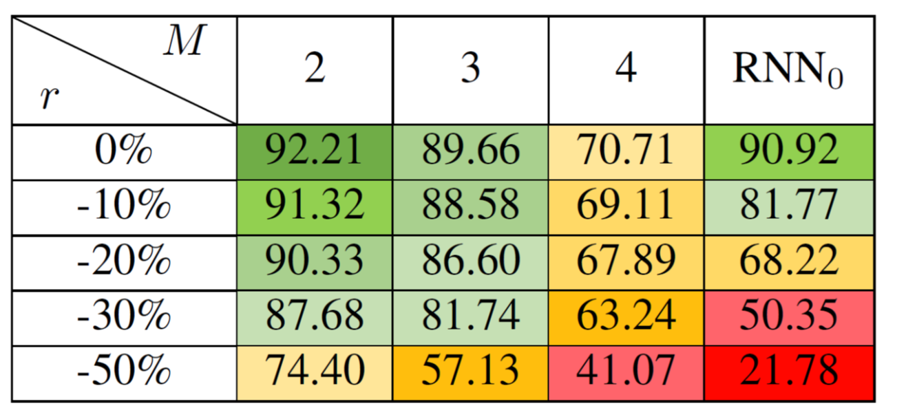
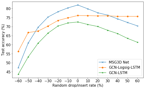
Figure 4: The accuracy (%) on the new test sets with various drop/insert rates ($r$). (Left) Chalearn2013. $N=4$, and no data augmentation is used. (Right) NTU RGB+D 120 data.

5.4 Efficiency Analysis

To demonstrate that the log-signature can help reduce the computational cost of backpropagating through many timesteps associated with RNN-type models we compare the training time and accuracy of a standard single LSTM block with a Logsig-LSTM using the same LSTM component on the ChaLearn dataset. To evaluate the efficiency as the length of the input sequence grows we linearly interpolate between frames to generate longer input sequences. We can see in the results in Figure 5 that, as the length of the input sequence grows, the time to train the Logsig-LSTM grows much slower than that of the standard LSTM. Moreover, the Logsig-LSTM retains its accuracy while the accuracy of the LSTM drops significantly as the input length increases. This shows that the addition of the log-signature helps with capturing long-range dependencies in the data by efficiently summarizing local time intervals and thus reducing the number of timesteps in the LSTM.

We also compare the performance of the log signature and the discrete cosine transformation (DCT), which was used in Mao et al. (2019) for reduction of the temporal dimension. Both transformations can be computed as a pre-processing step. As can be seen in Figure 5 in this case the log-signature leads to slightly longer training time than DCT due to a larger spatial dimension, but achieves a considerably higher accuracy. If the transformation is computed at training time the cost of DCT is comparable to the log-signature.

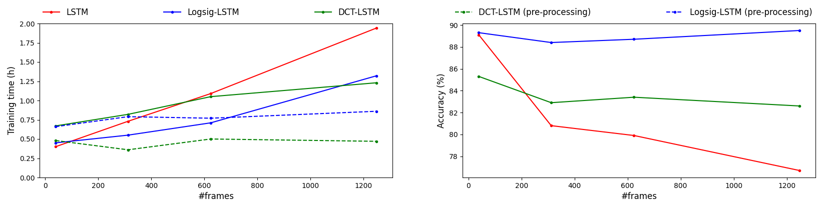
Figure 5: Comparison of training time and accuracy of standard LSTM and Logsig-LSTM.

6 Conclusion

We propose an efficient and compact end-to-end EL-Logsig-RNN network for SHAR tasks, providing a consistent performance boost of the SOTA models by replacing the RNN with the Logsig-RNN. As an enhancement of the RNN layer, the proposed Logsig-RNN module can reduce the time dimension, handle irregular time series and improve the robustness against missing data and varying frame rates. In particular, EL-Logsig-RNN achieves SOTA accuracy on Chalearn2013 for gesture recognition. For large-scale action data, the GCN-Logsig-RNN based models significantly improve the performance of EL-Logsig-RNN. Our model shows better robustness in handling varying frame rates. It merits further research to improve the combination with GCN-based models to further improve the accuracy while maintaining robustness.

Appendix

The (log)-signature of a path is a core mathematical object in rough path theory, which is a branch of stochastic analysis. In this appendix, we give a brief overview of the signature and log signature of a path, and their properties which are useful in the context of machine learning. Besides we provide illustrative examples via the python notebook in the supplementary material. In the following, for concreteness, we focus on paths of bounded variation, but the definition of the signature can be generalized to paths of finite $p$-variation. Interested readers can refer to Lyons et al. (2007) for a rigorous introduction of the (log)-signature of a path.

Appendix A The signature of a path

Let us recall the definition of the signature of a path. Let $J:=[S,T]$ denote a compact interval and $E:=\mathbb{R}^{d}$. $BV(J,E)$ denotes the space of all continuous paths of finite length from $J$ to $E$.

Definition A.1 (The Signature of a Path).

Let $X\in BV(J,E)$. Let $I=(i_{1},i_{2},\cdots,i_{n})$ be a multi-index of length $n$ where $i_{j}\in\{1,\cdots,d\},\forall j\in\{1,\cdots,n\}$. Define the coordinate signature of the path $X_{J}$ associated with the index $I$ as follows:

$$X^{I}_{J}=\underset{\underset{u_{1},\dots,u_{k}\in J}{u_{1}<\dots<u_{k}}}{\int\dots\int}dX_{u_{1}}^{(i_{1})}\dots dX_{u_{n}}^{(i_{2})}.$$

The signature of $X$ is defined as follows:

$$S(X)_{J}=(1,\mathbf{X}_{J}^{1},\dots,\mathbf{X}_{J}^{k},\dots)$$ (2)

where $\displaystyle\mathbf{X}_{J}^{k}=\underset{\underset{u_{1},\dots,u_{k}\in J}{u_{1}<\dots<u_{k}}}{\int\dots\int}dX_{u_{1}}\otimes\dots\otimes dX_{u_{k}}=(X^{I}_{J})_{I=(i_{1},\cdots,i_{k})},\forall k\geq 1$.

Let $S_{k}(X)_{J}$ denote the truncated signature of $X$ of degree $k$, i.e.

$$S_{k}(X)_{J}=(1,\mathbf{X}_{J}^{1},\dots,\mathbf{X}_{J}^{k}).$$ (3)

The signature of a path has a geometric interpretation. The first level signature $\mathbf{X}_{J}^{1}$ is the increment of the path $X$, i.e. $X_{T}-X_{S}$, while the second level signature represents the signed area enclosed by the curve $X$ and the cord connecting the start and end points of the path $X$.

The signature of $X$ arises naturally as the basis function to represent the solution to linear controlled differential equation based on the Picard’s iteration Lyons (1998). It plays the role of non-commutative monomials on the path space. In particular, if $X$ is a one-dimensional path, the $k^{th}$ level of the signature of $X$ can be computed explicitly by induction for every $k\in\mathbb{N}$ as follows

$$\mathbf{X}_{J}^{k}=\frac{(X_{T}-X_{S})^{k}}{k!}.$$ (4)

The signature of a $d$-dimensional linear path is given explicitly in the below lemma.

Lemma A.1.

Let $X:[S,T]\rightarrow E$ be a linear path. Then

$$S^{n}(X)=\frac{(X_{T}-X_{S})^{\otimes n}}{n!}.$$ (5)

Equivalently speaking, for any multi-index $I=(i_{1},\cdots,i_{n})$,

$$S^{I}=\frac{\prod_{j=1}^{n}(X_{T}^{(i_{j})})}{n!}.$$ (6)

The signature of a path can be interpreted as a solution to the controlled differential equation driven by a path in the tensor algebra space.

Theorem A.1.

Lyons et al. (2007) Let $X\in BV([0,T],E)$. Define $f:T^{(n)}\rightarrow L(E,T^{n}(E))$ by

$$f(a_{0},a_{1},\cdots,a_{n})x=(0,a_{0}\otimes x,a_{1}\otimes x,\cdots,a_{n-1}\otimes x).$$ (7)

Then the unique solution to the differential equation

$$dS_{t}=f(S_{t})dX_{t},S_{0}=(1,0,\cdots,0),$$ (8)

is the path $S:[0,T]\rightarrow T^{(n)}(E)$ defined for all $t\in[0,T]$ by

$$S_{t}=S_{n}(X_{[0,t]})=(1,\mathbf{X}_{[0,t]}^{1},\dots,\mathbf{X}_{[0,t]}^{n})).$$

Formally the signature of the path $X_{0,t}$ as a function from $[0,T]$ to $T((E))$ is the solution to the following equation

$$dS(X)_{[0,t]}=S(X_{[0,t]})\otimes dX_{t},S(X_{[0,0]})=1.$$

A.1 Multiplicative Property

The signature of paths of finite length (bounded variation) has the multiplicative property, also called Chen’s identity.

Definition A.2.

Let $X\in BV([0,s],E)$ and $Y\in BV([s,t],E)$ be two continuous paths. Their concatenation is the path denoted by $X*Y\in BV([0,t],E)$ defined by

$$(X*Y)_{u}=\begin{cases}X_{u},&u\in[0,s],\\ Y_{u}-Y_{s}+X_{s},&u\in[s,t].\end{cases}$$

Theorem A.2 (Chen’s identity).

. Let $X\in BV([0,s],E)$ and $Y\in BV([s,t],E)$. Then

$$S(X*Y)=S(X)\otimes S(Y).$$

Chen’s identity asserts that the signature is a homomorphism between the path space and the signature space.

The multiplicative properties of the signature allows us to compute the truncated signature of a piecewise linear path.

Lemma A.2.

Let $X$ be a $E$-valued piecewise linear path, i.e. $X$ is the concatenation of a finite number of linear paths, and in other words there exists a positive integer $l$ and linear paths $X_{1},X_{2},\cdots,X_{l}$ such that $X=X_{1}*X_{2}*\cdots*X_{l}$. Then

$$S(X)=\otimes_{i=1}^{l}\exp(X_{i}).$$ (9)

A.2 Uniqueness of the signature

Let us start with introducing the definition of the tree-like path.

Definition A.3 (Tree-like Path).

A path $X\in BV(J,E)$ is tree-like if there exists a continuous function $h:J\rightarrow[0,+\infty)$ such that $h(S)=h(T)=0$ and such that, for all $s,t\in J$ with $s\leq t$,

$$||X_{t}-X_{s}||\leq h(s)+h(t)-2\inf_{u\in[s,t]}h(u).$$

Intuitively a tree-like path is a trajectory in which there is a section where the path exactly retraces itself. The tree-like equivalence is defined as follows: we say that two paths $X$ and $Y$ are the same up to the tree-like equivalence if and only if the concatenation of $X$ and the inverse of $Y$ is tree-like. Now we are ready to characterize the kernel of the signature transformation.

Theorem A.3 (Uniqueness of the signature).

Let $X\in BV(J,E)$ . Then $S(X)$ determines $X$ up to the tree-like equivalence defined in Definition A.3.Hambly and Lyons (2010)

Theorem A.3 shows that the signature of the path can recover the path trajectory under a mild condition. The uniqueness of the signature is important, as it ensures it to be a discriminative feature set of un-parameterized streamed data.

Remark A.1.

A simple sufficient condition for the uniqueness of the signature of a path of finite length is that one component of $X$ is monotone. Thus the signature of the time-joint path determines its trajectory (see Levin et al. (2013)).

A.3 Invariance under time parameterization

Lemma A.3 (Invariance under time parameterization).

Lyons et al. (2007) Let $X\in V_{1}(J,E)$ and a path $\tilde{X}:J\rightarrow E$ be a time re-parameterization of $X$. Then

$$S(X_{J})=S(\tilde{X}_{J}).$$ (10)

Re-parameterizing a path inside the interval does not change its signature. As can be seen in Figure 2, speed changes result in different time series representation but the same signature feature. It means that signature feature can reduce dimension massively by removing the redundancy caused by the speed of traversing the path. It is very useful for applications where the output is invariant w.r.t. the speed of an input path, e.g. online handwritten character recognition and video classification.

A.4 Shuffle Product Property

We introduce a special class of linear forms on $T((E))$; Suppose $(e^{*}_{n_{1}},\cdots,e^{*}_{n_{d}},\cdots)$ are elements of $E^{*}$. We can introduce coordinate iterated integrals by setting $X^{(i)}_{u}:=\langle e^{*}_{i},X_{u}\rangle$, and rewriting $\langle e_{i_{1}}^{*}\otimes\cdots\otimes e_{i_{n}}^{*},S(X)\rangle$ as the scalar iterated integral of coordinate projection. In this way, we realize the $n^{th}$ degree coordinate iterated integrals as the restrictions of linear functionals in $E^{\otimes n}$ to the space of signatures of paths. If $(e_{1},\cdots,e_{d})$ is a basis for a finite dimensional space $E$, and $(e_{1}^{*},\cdots,e_{d}^{*})$ is a basis for the dual $E^{*}$ it therefore follows that

$$\mathbf{X}_{J}=\sum_{\begin{subarray}{c}k\geq 0\\ i_{1},\cdots,i_{k}\\ \in 1,2,\cdots,d\}\end{subarray}}\underset{\underset{u_{1},\dots,u_{k}\in J}{u_{1}<\dots<u_{k}}}{\int\dots\int}dX_{u_{1}}^{(i_{1})}\otimes\dots\otimes dX_{u_{k}}^{(i_{k})}e_{n_{1}}\otimes\cdots\otimes e_{n_{k}}.$$

Theorem A.4 (Shuffle Algebra).

The linear forms on $T((E))$ induced by $T(E^{*})$, when restricted to the range $S(BV([0,T],E)$ of the signature, form an algebra of real valued functions of bounded variation.

The proof can be found in page 35 in Lyons et al. (2007). The proof is based on the Fubini theorem, and it is to show that for any $e^{*},f^{*}\in T(E^{*})$, such that for all $\mathbf{a}\in S(\mathcal{V}^{p}([0,T],E)$,

$$e^{*}(\mathbf{a})f^{*}(\mathbf{a})=(e^{*}\shuffle f^{*})(\mathbf{a})$$ (11)

A.5 Universality of the signature

Any functional on the path can be rewritten as a function on the signature based on the uniqueness of the signature (Theorem A.3). The signature of the path has the universality property, i.e. that any continuous functional on the signature can be well approximated by linear functionals on the signature (Theorem A.5)Levin et al. (2013).

Theorem A.5 (Signature Approximation Theorem).

Suppose $f:S_{1}\rightarrow\mathbb{R}$ is a continuous function, where $S_{1}$ is a compact subset of $S(BV(J,E))$. Then $\forall\varepsilon>0$, there exists a linear functional $L\in T((E))^{*}$ such that

$$\sup_{a\in S_{1}}||f(a)-L(a)||\leq\varepsilon.$$ (12)

Proof.

It can be proved by the shuffle product property of the signature and the Stone-Weierstrass Theorem. ∎

Appendix B The log-signature of a path

Before introducing the log-signature, we define the Lie algebra, which the log-signature takes value in.

B.1 Lie algebra and Lie series

If $F_{1}$ and $F_{2}$ are two linear subspaces of $T((E))$, let us denote by $[F_{1},F_{2}]$ the linear span of all the elements of the form $[a,b]$, where $a\in F_{1}$ and $b\in F_{2}$. Consider the sequence $(L_{n})_{n\geq 0}$ of subspaces of $T((E))$ defined recursively as follows:

$$L_{0}=0;\forall n\geq 1,L_{n}=[E,L_{n-1}].$$ (13)

Definition B.1.

The space of Lie formal series over $E$, denoted as $\mathcal{L}((E))$ is defined as the following subspace of $T((E))$:

$$\mathcal{L}((E))=\{l=(l_{0},\cdots,l_{n},\cdots)|\forall n\geq 0,l_{n}\in L_{n}\}.$$ (14)

Theorem B.1 (Theorem 2.23 Lyons et al. (2007)).

Let $X\in BV(J,E)$. Then the log-signature of $X$ is a Lie series in $\mathcal{L}((E))$.

B.2 The bijection between the signature and log-signature

Similar to the way of defining the logarithm of a tensor series, we have the exponential mapping of the element in $T((E))$ defined in a power series form.

Definition B.2 (Exponential map).

Let $a=(a_{0},a_{1},\cdots)\in T((E))$. Define the exponential map denoted by $\exp$ as follows:

$$\exp(a)=\sum_{n=0}^{\infty}\frac{a^{\otimes n}}{n!}.$$ (15)

Lemma B.1.

The inverse of the logarithm on the domain $\{a\in T((E))|a_{0}\neq 0\}$ is the exponential map.

Theorem B.2.

The dimension of the space of the truncated log signature of $d$-dimensional path up to degree $n$ over $d$ letters is given by:

$$\mathcal{DL}_{n}=\frac{1}{n}\sum_{d|n}\mu(d)q^{n|d}$$

where $\mu$ is the Mobius function, which maps $n$ to

$$\left\{\begin{array}[]{ll}0,&\mbox{if $n$ has one or more repeated prime factors}\\ 1,&\mbox{if $n=1$}\\ (-1)^{k}&\mbox{if $n$ is the product of k distinct prime numbers}\end{array}\right.$$

The proof can be found in Corollary 4.14 p. 96 of Reutenauer (2003).

B.3 Calculation of the log-signature

Let’s start with a linear path. The log signature of a linear path $X_{J}$ is nothing else, but the increment of the path $X_{T}-X_{S}$.

The Baker-Cambpell-Hausdorff (BCH) formula gives a general method to compute the log-signature of the concatenation of two paths, which uses the multiplicativity of the signature and the free Lie algebra. It provides a way to compute the log-signature of a piecewise linear path by induction.

Theorem B.3.

For any $S_{1},S_{2}\in\mathcal{L}((E))$

$$Z=log(e^{S_{1}}e^{S_{2}})=\sum_{\begin{subarray}{c}n\geq 1\\ p_{1},...,p_{n}\geq 0\\ q_{1},....q_{n}\geq 0\\ p_{i}+q_{i}>0\end{subarray}}\frac{(-1)^{n+1}}{n}\frac{1}{p_{1}!q_{1}!...p_{n}!q_{n}!}r(S_{1}^{p_{1}}S_{2}^{q_{1}}...S_{1}^{p_{n}}S_{2}^{q_{n}})$$ (17)

where $r:A^{*}\rightarrow A^{*}$ is the right-Lie-bracketing operator, such that for any word $w=a_{1}...a_{n}$

$$r(w)=[a_{1},...,[a_{n-1},a_{n}]...].$$

This version of BCH is sometimes called the Dynkin’s formula.

Proof.

See remark of appendix 3.5.4 p. 81 in Reutenauer (2003). ∎

B.4 Uniqueness of the log-signature

Like the signature, the log-signature has the uniqueness stated in the following theorem.

Theorem B.4 (Uniqueness of the log-signature).

Let $X\in BV(J,E)$ . Then $lS(X)$ determines $X$ up to the tree-like equivalence defined in Definition A.3.

Theorem B.4 shows that the signature of the path can recover the path trajectory under a mild condition.

Lemma B.2.

A simple sufficient condition for the uniqueness of the log-signature of a path of finite length is that one component of $X$ is monotone.

Appendix C Comparison of the Signature and Log-signature

Both the signature and log-signature take the functional view on discrete time series data, which allows a unified way to treat time series of variable length and missing data. For example, we chose one pen-digit data of length 53 and simulate 1000 samples of modified pen trajectories by dropping at most 16 points from it, to mimic the missing data of variable length case (See one example in Figure 6). Figure 7 shows that the mean absolute relative error of the signature and log-signature of the missing data is no more than $6\%$. Besides, the log-signature feature is more robust against missing data, and it is of lower dimension compared with the signature feature.

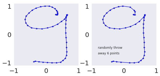
Figure 6: (Left) The chosen pen trajectory of digit 9. (Right) The simulated path by randomly dropping at most 16 points of the pen trajectory on the left.

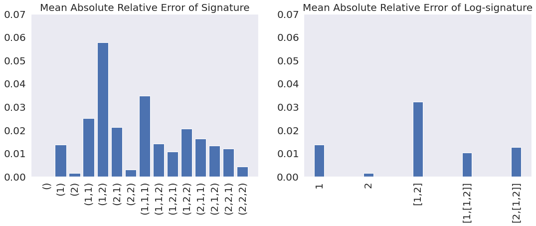
Figure 7: Signature and Log-Signature Comparison for the missing data case.

Figure 8: Signature and Log-Signature Comparison for the missing data case.

Appendix D Backpropagation of the Log-Signature Layer

In this section, we provide the detailed derivation of backpropagation through time in our paper. Following the notations in Section 4 of our paper, $l_{k}:=l_{k}^{M}$ denotes the log-signatures of a path $x^{\hat{\mathcal{D}}}$ over time partition $[u_{k},u_{k+1}]$ of degree $M$. Let us consider the derivative of the scalar function $F$ on $(l_{k})_{k=1}^{N}$ with respect to path $x^{\hat{\mathcal{D}}}$, given the derivatives of $F$ with respect to $(l_{k})_{k=1}^{N}$. W.l.o.g assume that $\hat{\mathcal{D}}\subset\mathcal{D}$. By the Chain rule, it holds that

$$\frac{\partial F((l_{1},\cdots,l_{N}))}{\partial x_{t_{i}}}=\sum_{k=1}^{N}\frac{\partial F(l_{1},\cdots,l_{N})}{\partial l_{k}}\frac{\partial l_{k}}{\partial x_{t_{i}}}.$$ (18)

where $k\in\{1,\cdots,N\}$ and $i\in\{0,1,\cdots,n\}$.

If $t_{i}\notin[u_{k-1},u_{k}]$, $\frac{\partial l_{k}}{\partial x_{t_{i}}}=0;$ otherwise $\frac{\partial l_{k}}{\partial x_{t_{i}}}$ is the derivative of the single log-signature $l_{k}$ with respect to path $x_{u_{k-1},u_{k}}$ where $t_{i}\in\mathcal{D}\cap[u_{k-1},u_{k}]$. The log signature $lS(x^{\hat{\mathcal{D}}})$ with respect to $x_{t_{i}}$ is proved differentiable and the algorithm of computing the derivatives is given in Jeremy (2019), denoted by $\triangledown_{x_{t_{i}}}LS(x^{\hat{\mathcal{D}}})$. This is a special case for our log-signature layer when $N=1$. In general, for any $N\in\mathbb{Z}^{+}$, it holds that $\forall i\in\{0,1,\cdots,n\}$ and $k\in\{1,\cdots,N\}$,

$$\frac{\partial l_{k}}{\partial x_{t_{i}}}=\mathbf{1}_{t_{i}\in[u_{k-1},u_{k}]}\triangledown_{x_{t_{i}}}LS(x_{u_{k-1},u_{k}}).$$ (19)

The backpropagation of the Log-Signature Layer can be implemented using Equation (18) and (19).

Appendix E Other Path Transformation Layers

In this section, we introduce two other useful Path Transformation Layers which are often accompanied with the Embedding Layer in the PT-Logsig-RNN to improve the performance.

Accumulative Layer. Accumulative Layer (AL) maps the input sequence $(X_{t_{i}})_{i=1}^{n}$ to its partial sum sequence $Y_{t_{i}}$, where $Y_{t_{i}}=\sum_{j=1}^{i}X_{t_{j}}$, and $i=1,\cdots,n$. One advantage of using the Accumulative Layer along with Log-Signature Layer is to extract the quadratic variation and other higher order statistics of an input path $X$ effectively Ni (2015).

Time-incorporated Layer. Time-incorporated Layer (TL) is to add the time dimension to the input $(X_{t_{i}})_{i=1}^{n}$; in formula, the output is $(t_{i},X_{t_{i}})_{i=1}^{n}$. As speed information is informative in most of SHAR tasks, e.g. distinguish running and walking, the log-signature of the time-incorporated transformation of a path can preserve such information.

Appendix F Numerical Experiments

Network Architecture of PT-Logsig-RNN on Chalearn2013 data can be found in Table 3.

Layer		Output shape	Description
Input		$(n,20,3)$	Input with $n$ time steps
	Conv2D	$(n,20,32)$	Kernel size=$1\times 1\times 32$
Embedding	Conv2D	$(n,20,16)$	Kernel size=$3\times 1\times 16$
Layer	Flatten	$(n,320)$	Flatten spatial dimensions
	Conv1D	$(n,30)$	Kernel size=$1\times 304\times 30$
Accumulative Layer (AL)		$(n,30)$	Partial sum on the series
Time-incorporated Layer (TL)		$(n,31)$	Add temporal dimension
Logsig Layer		$(N,496)$	$M=2,N=4$ after tuning
Add Starting Points		$(N,527)$	Starting points of TL output
LSTM		$(N,128)$	Return sequential output
Output		$20$

Table 3: Architecture of the PT-Logsig-RNN on Chalearn 2013

References

- Lo Presti and La Cascia [2016] Liliana Lo Presti and Marco La Cascia. 3d skeleton-based human action classification. Pattern Recognition, 53(C):130–147, 2016.
- Wang et al. [2019a] Lei Wang, Du Q Huynh, and Piotr Koniusz. A comparative review of recent kinect-based action recognition algorithms. IEEE Transactions on Image Processing, 29:15–28, 2019a.
- Ren et al. [2020] Bin Ren, Mengyuan Liu, Runwei Ding, and Hong Liu. A survey on 3d skeleton-based action recognition using learning method. arXiv preprint arXiv:2002.05907, 2020.
- Lev et al. [2016] Guy Lev, Gil Sadeh, Benjamin Klein, and Lior Wolf. Rnn fisher vectors for action recognition and image annotation. In European Conference on Computer Vision, pages 833–850. Springer, 2016.
- Liu et al. [2016] Jun Liu, Amir Shahroudy, Dong Xu, and Gang Wang. Spatio-temporal lstm with trust gates for 3d human action recognition. In ECCV, pages 816–833, 2016. ISBN 978-3-319-46487-9.
- Liu et al. [2018] Jun Liu, Guanghui Wang, Ling yu Duan, Kamila Abdiyeva, and Alex ChiChung Kot. Skeleton-based human action recognition with global context-aware attention lstm networks. IEEE TIP,, 27:1586–1599, 2018.
- Shahroudy et al. [2016] Amir Shahroudy et al. Ntu rgb+d: A large scale dataset for 3d human activity analysis. In CVPR, 06 2016. doi:10.1109/CVPR.2016.115.
- Wang and Wang [2017] Hongsong Wang and Liang Wang. Modeling temporal dynamics and spatial configurations of actions using two-stream recurrent neural networks. CVPR,, pages 3633–3642, 2017.
- Caetano et al. [2019] Carlos Caetano, Jessica Sena, François Brémond, Jefersson A Dos Santos, and William Robson Schwartz. Skelemotion: A new representation of skeleton joint sequences based on motion information for 3d action recognition. In 2019 16th IEEE International Conference on Advanced Video and Signal Based Surveillance (AVSS), pages 1–8. IEEE, 2019.
- Chéron et al. [2015] Guilhem Chéron, Ivan Laptev, and Cordelia Schmid. P-cnn: Pose-based cnn features for action recognition. In Proceedings of the IEEE international conference on computer vision, pages 3218–3226, 2015.
- Ke et al. [2018] Q. Ke, M. Bennamoun, S. An, F. Sohel, and F. Boussaid. Learning clip representations for skeleton-based 3d action recognition. IEEE TIP,, 27(6):2842–2855, June 2018. ISSN 1057-7149. doi:10.1109/TIP.2018.2812099.
- Li et al. [2018] Chao Li, Qiaoyong Zhong, Di Xie, and Shiliang Pu. Co-occurrence feature learning from skeleton data for action recognition and detection with hierarchical aggregation. In Proceedings of the 27th International Joint Conference on Artificial Intelligence, pages 786–792, 2018.
- Liu et al. [2019a] Jun Liu, Amir Shahroudy, Gang Wang, Ling-Yu Duan, and Alex C. Kot. Skeleton-based online action prediction using scale selection network. IEEE TPAMI, 02 2019a. doi:10.1109/TPAMI.2019.2898954.
- Liu and Yuan [2018] Mengyuan Liu and Junsong Yuan. Recognizing human actions as the evolution of pose estimation maps. In CVPR, pages 1159–1168, 2018.
- Li et al. [2019a] Maosen Li, Siheng Chen, Xu Chen, Ya Zhang, Yanfeng Wang, and Qi Tian. Actional-structural graph convolutional networks for skeleton-based action recognition. In Proceedings of the IEEE Conference on Computer Vision and Pattern Recognition, pages 3595–3603, 2019a.
- Shi et al. [2019] Lei Shi, Yifan Zhang, Jian Cheng, and Hanqing Lu. Skeleton-based action recognition with directed graph neural networks. In Proceedings of the IEEE Conference on Computer Vision and Pattern Recognition, pages 7912–7921, 2019.
- Fan et al. [2016] Jiayi Fan, Zhengjun Zha, and Xinmei Tian. Action recognition with novel high-level pose features. In 2016 IEEE International Conference on Multimedia & Expo Workshops (ICMEW), pages 1–6. IEEE, 2016.
- Jhuang et al. [2013] Hueihan Jhuang, Juergen Gall, Silvia Zuffi, Cordelia Schmid, and Michael J Black. Towards understanding action recognition. In Proceedings of the IEEE international conference on computer vision, pages 3192–3199, 2013.
- Yang and Tian [2014] Xiaodong Yang and YingLi Tian. Effective 3d action recognition using eigenjoints. Journal of Visual Communication and Image Representation, 25(1):2–11, 2014.
- Evangelidis et al. [2014] Georgios Evangelidis, Gurkirt Singh, and Radu Horaud. Skeletal quads: Human action recognition using joint quadruples. In 2014 22nd International Conference on Pattern Recognition, pages 4513–4518. IEEE, 2014.
- Li and Leung [2016] Meng Li and Howard Leung. Multiview skeletal interaction recognition using active joint interaction graph. IEEE Transactions on Multimedia, 18(11):2293–2302, 2016.
- Shahroudy et al. [2015] Amir Shahroudy, Tian-Tsong Ng, Qingxiong Yang, and Gang Wang. Multimodal multipart learning for action recognition in depth videos. IEEE transactions on pattern analysis and machine intelligence, 38(10):2123–2129, 2015.
- Ke et al. [2017] Qiuhong Ke, Senjian An, Mohammed Bennamoun, Ferdous Sohel, and Farid Boussaid. Skeletonnet: Mining deep part features for 3-d action recognition. IEEE signal processing letters, 24(6):731–735, 2017.
- Liu et al. [2020] Z. Liu, H. Zhang, Z. Chen, Z. Wang, and W. Ouyang. Disentangling and unifying graph convolutions for skeleton-based action recognition. In 2020 IEEE/CVF Conference on Computer Vision and Pattern Recognition (CVPR), pages 140–149, 2020. doi:10.1109/CVPR42600.2020.00022.
- Lyons [1998] Terry J Lyons. Differential equations driven by rough signals. Revista Matemática Iberoamericana,, 14(2):215–310, 1998.
- Levin et al. [2013] Daniel Levin, Terry Lyons, and Hao Ni. Learning from the past, predicting the statistics for the future, learning an evolving system. arXiv preprint arXiv:1309.0260, 2013.
- Gyurkó et al. [2013] Lajos Gergely Gyurkó, Terry Lyons, Mark Kontkowski, and Jonathan Field. Extracting information from the signature of a financial data stream. arXiv preprint arXiv:1307.7244, 2013.
- Lyons et al. [2014] Terry Lyons, Hao Ni, and Harald Oberhauser. A feature set for streams and an application to high-frequency financial tick data. In ACM International Conference on Big Data Science and Computing, page 5, 2014.
- Diehl [2013] Joscha Diehl. Rotation invariants of two dimensional curves based on iterated integrals. arXiv preprint arXiv:1305.6883, 2013.
- Graham [2013] Benjamin Graham. Sparse arrays of signatures for online character recognition. arXiv preprint arXiv:1308.0371, 2013.
- Yang et al. [2016a] Weixin Yang, Lianwen Jin, Dacheng Tao, Zecheng Xie, and Ziyong Feng. Dropsample: A new training method to enhance deep convolutional neural networks for large-scale unconstrained handwritten chinese character recognition. Pattern Recognition, 58:190–203, 2016a.
- Xie et al. [2018] Zecheng Xie, Zenghui Sun, Lianwen Jin, Hao Ni, and Terry Lyons. Learning spatial-semantic context with fully convolutional recurrent network for online handwritten chinese text recognition. IEEE TPAMI,, 40(8):1903–1917, 2018.
- Yang et al. [2016b] Weixin Yang, Lianwen Jin, and Manfei Liu. Deepwriterid: An end-to-end online text-independent writer identification system. IEEE Intelligent Systems, 31(2):45–53, 2016b.
- Lai et al. [2017] Songxuan Lai, Lianwen Jin, and Weixin Yang. Online signature verification using recurrent neural network and length-normalized path signature descriptor. In 2017 14th IAPR International Conference on Document Analysis and Recognition (ICDAR), volume 1, pages 400–405. IEEE, 2017.
- Arribas et al. [2018] Imanol Perez Arribas, Guy M Goodwin, John R Geddes, Terry Lyons, and Kate EA Saunders. A signature-based machine learning model for distinguishing bipolar disorder and borderline personality disorder. Translational psychiatry, 8(1):1–7, 2018.
- Wang et al. [2019b] Bo Wang, Maria Liakata, Hao Ni, Terry Lyons, Alejo J Nevado-Holgado, and Kate Saunders. A path signature approach for speech emotion recognition. In Interspeech 2019, pages 1661–1665. ISCA, 2019b.
- Ahmad et al. [2019] Tasweer Ahmad, Lianwen Jin, Jialuo Feng, and Guozhi Tang. Human action recognition in unconstrained trimmed videos using residual attention network and joints path signature. IEEE Access, 7:121212–121222, 2019.
- Király and Oberhauser [2016] Franz J Király and Harald Oberhauser. Kernels for sequentially ordered data. arXiv preprint arXiv:1601.08169, 2016.
- Li et al. [2019b] Chenyang Li, Xin Zhang, Lufan Liao, Lianwen Jin, and Weixin Yang. Skeleton-based gesture recognition using several fully connected layers with path signature features and temporal transformer module. In AAAI, pages 8585–8593, 2019b.
- Yang et al. [2017] Weixin Yang, Terry Lyons, Hao Ni, Cordelia Schmid, Lianwen Jin, and Jiawei Chang. Leveraging the path signature for skeleton-based human action recognition. arXiv preprint arXiv:1707.03993, 2017.
- Li et al. [2017] Chenyang Li, Xin Zhang, and Lianwen Jin. Lpsnet: A novel log path signature feature based hand gesture recognition framework. In 2017 IEEE International Conference on Computer Vision Workshops (ICCVW), pages 631–639, 2017. doi:10.1109/ICCVW.2017.80.
- Kidger et al. [2021] Patrick Kidger, James Morrill, James Foster, and Terry Lyons. Neural controlled differential equations for irregular time series. In International Conference on Machine Learning (ICML), 2021.
- Kidger et al. [2019] Patrick Kidger, Patric Bonnier, Imanol Perez Arribas, Cristopher Salvi, and Terry Lyons. Deep signature transforms. In Advances in Neural Information Processing Systems, volume 32, 2019.
- Chevyrev and Kormilitzin [2016] Ilya Chevyrev and Andrey Kormilitzin. A primer on the signature method in machine learning. arXiv preprint arXiv:1603.03788, 2016.
- [45] Terry Lyons, Djalil Chafai, Stephen Buckley, Greg Gyurko, and Arend Janssen. Esig on pypi derived from coropa: Computational rough paths software library. https://github.com/datasig-ac-uk/esig,https://github.com/terrylyons/libalgebra, http://coropa.sourceforge.net/. [Online].
- Jeremy and Benjamin. [2018] Reizenstein Jeremy and Graham Benjamin. The iisignature library: efficient calculation of iterated-integral signatures and log signatures. arXiv preprint arXiv:1802.08252., 2018.
- Kidger and Lyons [2020] Patrick Kidger and Terry Lyons. Signatory: differentiable computations of the signature and logsignature transforms, on both cpu and gpu. arXiv preprint arXiv:2001.00706, 2020.
- Hambly and Lyons [2010] B.M. Hambly and Terry Lyons. Uniqueness for the signature of a path of bounded variation and the reduced path group. Annals of Mathematics,, 171(1):109–167, 2010.
- Reizenstein and Graham [2018] Jeremy Reizenstein and Benjamin Graham. The iisignature library: efficient calculation of iterated-integral signatures and log signatures. arXiv preprint arXiv:1802.08252, 2018.
- Escalera et al. [2013] Sergio Escalera, Jordi Gonzàlez, Xavier Baró, Miguel Reyes, Oscar Lopes, Isabelle Guyon, Vassilis Athitsos, and Hugo Jair Escalante. Multi-modal gesture recognition challenge 2013: dataset and results. In ICMI, 2013.
- Liu et al. [2019b] Jun Liu, Amir Shahroudy, Mauricio Perez, Gang Wang, Ling-Yu Duan, and Alex C. Kot. Ntu rgb+d 120: A large-scale benchmark for 3d human activity understanding. IEEE TPAMI, 2019b. doi:10.1109/TPAMI.2019.2916873.
- Liao et al. [2019] Lufan Liao, Xin Zhang, and Chenyang Li. Multi-path convolutional neural network based on rectangular kernel with path signature features for gesture recognition. In 2019 IEEE Visual Communications and Image Processing (VCIP), pages 1–4. IEEE, 2019.
- Liu et al. [2018] J. Liu, A. Shahroudy, D. Xu, A. C. Kot, and G. Wang. Skeleton-based action recognition using spatio-temporal lstm network with trust gates. IEEE TPAMI,, 40(12):3007–3021, Dec 2018. ISSN 0162-8828. doi:10.1109/TPAMI.2017.2771306.
- Song et al. [2021] Yi-Fan Song, Zhang Zhang, Caifeng Shan, and Liang Wang. Richly activated graph convolutional network for robust skeleton-based action recognition. IEEE Transactions on Circuits and Systems for Video Technology, 31(5):1915–1925, 2021. doi:10.1109/TCSVT.2020.3015051.
- Cheng et al. [2020] Ke Cheng, Yifan Zhang, Xiangyu He, Weihan Chen, Jian Cheng, and Hanqing Lu. Skeleton-based action recognition with shift graph convolutional network. In Proceedings of the IEEE/CVF Conference on Computer Vision and Pattern Recognition (CVPR), June 2020.
- Song et al. [2020] Yi-Fan Song, Zhang Zhang, Caifeng Shan, and Liang Wang. Stronger, faster and more explainable: A graph convolutional baseline for skeleton-based action recognition. In Proceedings of the 28th ACM International Conference on Multimedia, MM ’20, page 1625–1633, New York, NY, USA, 2020. Association for Computing Machinery. ISBN 9781450379885. doi:10.1145/3394171.3413802. URL https://doi.org/10.1145/3394171.3413802.
- Mao et al. [2019] Wei Mao, Miaomiao Liu, Mathieu Salzmann, and Hongdong Li. Learning trajectory dependencies for human motion prediction. In Proceedings of the IEEE/CVF International Conference on Computer Vision, pages 9489–9497, 2019.
- Lyons et al. [2007] Terry J Lyons, Michael Caruana, and Thierry Lévy. Differential equations driven by rough paths. Springer, 2007.
- Reutenauer [2003] Christophe Reutenauer. Free lie algebras. In Handbook of algebra, volume 3, pages 887–903. Elsevier, 2003.
- Jeremy [2019] Reizenstein Jeremy. Iterated-Integral Signatures in Machine Learning. PhD thesis, 2019.
- Ni [2015] Hao Ni. A multi-dimensional stream and its signature representation. arXiv preprint arXiv:1509.03346, 2015.