AxoNN: An asynchronous, message-driven parallel framework for extreme-scale deep learning

Abstract

In the last few years, the memory requirements to train state-of-the-art neural networks have far exceeded the DRAM capacities of modern hardware accelerators. This has necessitated the development of efficient algorithms to train these neural networks in parallel on large-scale GPU-based clusters. Since computation is relatively inexpensive on modern GPUs, designing and implementing extremely efficient communication in these parallel training algorithms is critical for extracting the maximum performance. This paper presents AxoNN, a parallel deep learning framework that exploits asynchrony and message-driven execution to schedule neural network operations on each GPU, thereby reducing GPU idle time and maximizing hardware efficiency. By using the CPU memory as a scratch space for offloading data periodically during training, AxoNN is able to reduce GPU memory consumption by four times. This allows us to increase the number of parameters per GPU by four times, thus reducing the amount of communication and increasing performance by over 13%. When tested against large transformer models with 12–100 billion parameters on 48–384 NVIDIA Tesla V100 GPUs, AxoNN achieves a per-GPU throughput of 49.4–54.78% of theoretical peak and reduces the training time by 22-37 days (15–25% speedup) as compared to the state-of-the-art.

I Introduction

In recent years, the field of deep learning has been moving toward training extremely large neural networks (NNs) for advancing the state-of-the-art in areas such as computer vision and natural language processing (NLP) [1, 2, 3]. This surge in popularity of large NNs has been propelled by the availability of large quantities of data and the increasing computational capabilities of hardware such as GPUs. However, the memory requirements to train such networks have far exceeded the DRAM capacities of modern hardware accelerators. This has necessitated the development of efficient algorithms to train neural networks in parallel on large-scale GPU-based clusters.

Computation is relatively inexpensive on modern GPUs and has outpaced the increase in network bandwidth on GPU-based clusters with size. Hence, the design and implementation of efficient communication algorithms is critical to prevent starvation of GPUs waiting for data to compute on. Contemporary frameworks for parallel deep learning suffer from a number of shortcomings in this regard. Some of them employ bulk synchronous parallel algorithms to divide the computation of each layer across GPUs [4, 2]. The synchronization step in these algorithms can be time-consuming as it employs collective communication on the outputs of each layer, which are fairly large in size. Other frameworks try to divide contiguous subsets of layers across GPUs [5, 6, 7]. Data is then exchanged between consecutive GPUs using point-to-point communication. In this setting, such implementations fail to exploit the potential of overlapping communication and computation due to the use of blocking communication primitives and static scheduling of layer operations.

In this paper, we present AxoNN, a parallel deep learning framework that exploits asynchrony and message-driven execution to schedule neural network operations on each GPU, thereby reducing GPU idle time and maximizing hardware efficiency. To achieve asynchronous message-driven execution, we implement AxoNN’s communication backend using CUDA-aware MPI with GPU-Direct support. While the general consensus among other frameworks [5, 6, 7] has been to use NCCL [8] or Gloo [9] for point-to-point communication, we find that MPI is more suitable for this task because it offers higher intra-node bandwidth and supports non-blocking primitives, which are great for asynchrony. This gives AxoNN an edge over other frameworks in terms of performance. To the best of our knowledge, this is the first work to exploit implement message-driven execution for parallel deep learning, with prior work using static scheduling schemes due to the constraints of synchronous communication.

Neural networks with extremely large number of parameters like the GPT-3 [3] architecture require a correspondingly large number of GPUs often ranging in the hundreds. At such large GPU counts, there is a notable drop in hardware efficiency due to increasing communication to computation ratios [5]. To mitigate this problem, AxoNN implements an intelligent memory optimization algorithm that enables it to reduce the number of GPUs required to train a single instance of a neural network by four times. This is made possible by using the CPU memory as a scratch space for offloading data periodically during training and prefetching it intelligently whenever required. To extend training to a large number of GPUs, we employ data parallelism wherein multiple instances of the neural network are trained in an embarrassingly parallel manner [10]. When evaluated against a 12 billion parameter transformer [11] neural network, our memory optimizations yield a performance improvement of over 13%.

We demonstrate the scalability of our implementation and compare its performance with that of existing state-of-the-art parallel deep learning frameworks - Megatron-LM [5] and DeepSpeed [6, 12]. Our experiments show that AxoNN comprehensively outperforms other frameworks in both weak scaling and strong scaling settings. When tested against large GPT-style [3] transformer models with 12, 24, 50 and 100 billion parameters on 48, 96, 192 and 384 NVIDIA Tesla V100 GPUs respectively, AxoNN achieves an impressive per-GPU throughput of 49.4–54.78% of theoretical peak and reduces the training time by 22-37 days as compared to the next best framework – DeepSpeed. Our framework can thus help researchers save time and resources in their experiments.

Our contributions can be summarized as follows:

• We propose a MPI-based point-to-point communication backend for parallel deep learning that exploits asynchrony to overlap communication with computation and thus increase hardware efficiency.

• We also implement a message-driven scheduler that enables the scheduling of neural network operations in the order in which their data dependencies are met.

• We develop a proof that explains the reasons for inefficiency of certain parallel deep learning algorithms at scale. We then propose a novel memory optimization algorithm that mitigates this issue by using the CPU memory as a scratch space to offload and prefetch data intelligently.

• We present a user-friendly, open-source implementation of AxoNN, which places minimal programming burden on the end-user, similar to the familiar single GPU PyTorch programming environment.

II Background on deep learning

This section provides a background on training neural networks, and different modes of parallelism in deep learning.

II-A Definitions and basics of training neural networks

We now describe the basic terminology and the layout of a typical neural network training procedure.

Neural networks: are parameterized function approximators. Their popularity stems from their flexibility to approximate a plethora of functions on high dimensional input data. The training algorithm iteratively adjusts the values of the parameters to fit the input data accurately. We collectively refer to the entire parameter vector of the neural network as $\vec{\theta}$.

Layers: Computation of a neural network is divided into layers. Each layer consumes the output of its previous layer. The first layer operates directly on the input. The output of the last layer is the final output of the neural network. The outputs of intermediate layer are called activations. We refer to a neural network with N layers as $(l_{0},l_{1},l_{2},...l_{N-1})$, where $l_{i}$ stands for the $i^{th}$ layer. $\vec{\theta_{i}}$ and $\vec{a_{i}}$ refer to the parameters and activations of the $i^{th}$ layer respectively.

Loss: is a scalar which defines how well a given set of parameters of a neural network $\vec{\theta}$ approximate the input dataset. The task of training is essentially a search for the value of $\vec{\theta}$, which minimizes the loss function - $L(X,\vec{\theta})$, where $X$ is the input dataset.

Forward and backward pass: A neural network first computes the activations for each layer and subsequently the loss function for a given $(X,\vec{\theta})$. This is called the forward pass. After that it computes the gradient of the loss w.r.t. the parameters i.e. $\nabla\vec{\theta}=\frac{dL(X,\vec{\theta})}{d\vec{\theta}}$ via the backpropagation algorithm [13]. This is called the backward pass.

Optimizer: The optimizer uses $\nabla\vec{\theta}$ to update $\vec{\theta}$ to a value that incrementally reduces the value of $L(X,\vec{\theta})$. A training run includes repeated forward pass, backward passes followed by the optimizer step to iteratively update $\vec{\theta}$ to a desirable value which fits the data better. Deep learning optimizers maintain a state vector $\vec{s_{opt}}$ of size $\mathcal{O}(|\vec{\theta}|)$ which is usually a running history of past gradient vectors. The updated $\vec{\theta}$ is a function of $\vec{s_{opt}}$ and $\nabla\vec{\theta}$.

Batch: Training algorithms do not use the entire dataset $X$ for computing the loss. Instead mutually exclusive and exhaustive subsets called batches of the dataset are repeatedly sampled for training. The cardinality of a batch is called the batch size.

Mixed precision: Mixed precision training involves keeping two copies of the network parameters in single and half precision [14]. Forward and backward passes are done in half precision to boost performance. However, the optimizer step is applied to the single precision copy of the weight. To prevent underflow during the calculation of half precision gradients, the loss is typically scaled up by multiplication with a large number called the scaling factor. The optimizer first converts the half precision gradients into full precision and then descales them to obtain their true value. Mixed precision computation can take advantage of the fast Tensor Cores present in modern hardware accelerators such as the NVIDIA V100 and A100 GPUs. We refer to half precision parameters and gradients as $\vec{\theta_{16}}$ and $\nabla\vec{\theta_{16}}$ respectively and their full precision counterparts as $\vec{\theta}$ and $\nabla\vec{\theta}$ respectively.

II-B Modes of parallelism in deep learning

Algorithms for parallel deep learning fall into three categories - data parallelism, intra-layer parallelism and inter-layer parallelism. Frameworks that rely on more than one kind of parallelism are said to be implementing hybrid parallelism.

Data parallelism: In data parallelism, identical copies of the model parameters are distributed among GPUs. Input batches are divided into equal sized chunks and consumed by individual GPUs for computation, which proceeds independently on each GPU. After that a collective all-reduce communication is initiated to average the parameter gradients on each rank. The average gradients are used to update the local copies of the network parameters. Due to its embarrassingly parallel nature, data parallelism scales very efficiently in practice. However, vanilla data parallelism is restricted by the need to fit the entire model in a single GPU. To overcome this restriction, it has to be combined with inter-layer and intra-layer parallelism for training extremely large neural networks such as GPT-3 [3].

Intra-layer parallelism: divides the computation of each layer of the neural network on multiple GPUs. Each GPU is responsible for partially computing the output activation of a layer. These partial outputs are pieced together using a collective communication primitive like all-gather or all-reduce to be used for the computation of the next layer. For example, Megatron-LM [2, 5] shards the various matrix multiplications of a transformer [11] layer across GPUs. While saving memory, it is prohibited by expensive collective communication after computing the output activations. Typically, intra-layer parallelism cannot scale efficiently beyond the confines of GPUs inside a node connected via a high-speed inter-connect like NVLink [5].

Inter-layer parallelism: divides the layers of a neural network among worker GPUs. To achieve parallelism, an input batch is divided into smaller microbatches. Forward and backward passes for different microbatches can thus proceed on different GPUs concurrently. Inter-layer parallelism is often called as pipelining and the set of GPUs implementing it are called the pipeline. Prior work has shown that inter-layer parallelism is inefficient for a large number of GPUs in the pipeline due to an increase in the idle time in the pipeline [5]. Figure 1 illustrates the working of inter-layer parallelism.

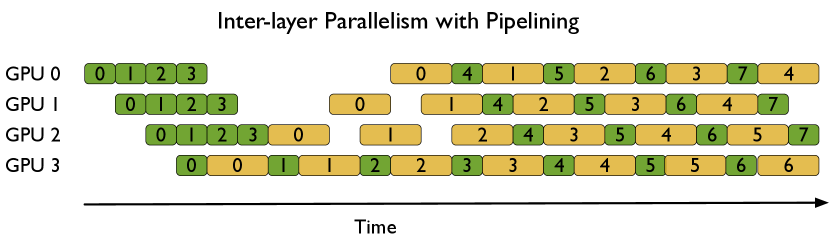
Figure 1: Inter-layer parallelism on four GPUs. The green and yellow boxes represent the forward and backward passes of a microbatch respectively. The numbers inside each box represent the microbatch number. We assume that the backward pass takes twice as much time as the forward pass.

Hybrid parallelism: Data parallelism is often combined with either or both of intra-layer or inter-layer parallelism to realize hybrid parallelism. For example, Megatron-LM [5] and DeepSpeed [12, 6] combine all three forms of parallelism to train large transformer neural networks [11] at extreme scale. This form of parallelism has been called 3D parallelism in literature. Prior work [15, 5] has shown 3D parallelism as the fastest method for training large scale neural networks.

III Designing a parallel deep learning framework

We now present the design of our new framework. AxoNN combines inter-layer parallelism and data parallelism to scale parallel training to a large number of GPUs.

III-A A hybrid approach to parallel training

The central idea behind AxoNN’s hybrid parallelization of neural networks is to create a hierarchy of compute resources (GPUs) by dividing them into equally sized groups. Each group of GPUs can be treated as a unit that has a full copy of the network similar to a single GPU in the case of pure data parallelism. Each group works on different shards of a batch concurrently to provide data parallelism. GPUs within each group are used to parallelize the computation associated with processing a batch shard using inter-layer parallelism. In the case of AxoNN, we arrange GPUs in a virtual 2D grid topology as shown in Figure 2. GPUs in each row form a group and are used to implement inter-layer parallelism within each group. The groups together are used to provide data parallelism by processing different shards of a batch in parallel. We use $\mathit{G_{data}}$ and $\mathit{G_{inter}}$ to denote the number of data-parallel groups and the number of GPUs inside each data-parallel group respectively.

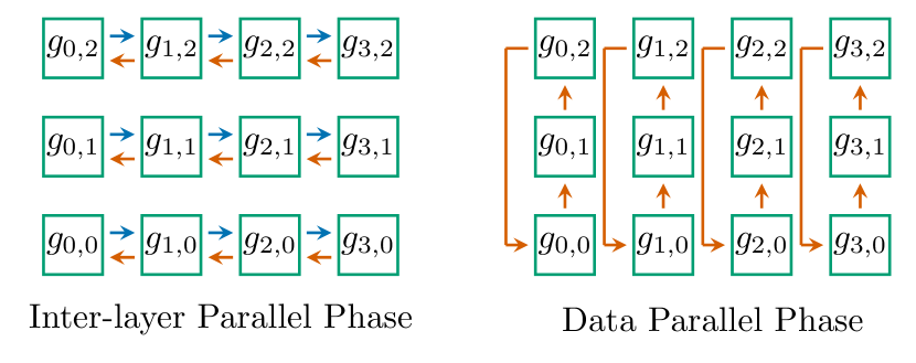
Figure 2: AxoNN uses hybrid parallelism that combines inter-layer and data parallelism. In this example, we train a neural network on 12 GPUs in a $4\times 3$ configuration (4-way inter-layer parallelism and 3-way data parallelism). The blue and red arrows represent communication of activations and gradients respectively. In inter-layer parallelism, these gradients are w.r.t. the output activations, whereas in data parallelism, these gradients are w.r.t. the network parameters.

Algorithm 1 AxoNN’s hybrid training algorithm for GPU $g^{i,j}$ in a $G_{\mathit{inter}}\times G_{\mathit{data}}$ configuration

1:function train(neural_network, dataset …)

2:    nn_shard $\leftarrow$ instantiate neural network shard for $g^{i,j}$

3:    while training has not finished do

4:         next_batch $\leftarrow$ get next batch from dataset

5:         batch_shard $\leftarrow$ get batch shard for $g^{i,j}$

6:         data_parallel_step(nn_shard, batch_shard …)

7:         run the optimizer

8:    end while

9:end function

10:

11:function data_parallel_step(nn_shard, batch_shard …)

12:    inter_layer_parallel_step(nn_shard, batch_shard …)

13:    All-reduce on nn_shard.$\nabla\vec{\theta}$

14:end function

Algorithm 1 explains the working of AxoNN’s parallel algorithm from the point of view of one of the GPUs $g^{i,j}$ in the 2D virtual grid. Training begins in the train function (line 1) which takes a neural network specification and a training dataset as its arguments. For each GPU, we first instantiate a neural network shard (contiguous subset of layers) that GPU $g^{i,j}$ will be responsible for in the inter-layer phase (line 12). In the main training loop (lines 3-7), we divide the input batch into $G_{\mathit{data}}$ shards (line 5) and run the data parallel step on the corresponding shard of $g^{i,j}$. The data parallel step first calls the inter-layer parallel step followed by an all-reduce on the gradients of the network shard. In the optimizer phase, we run a standard optimizer used in deep learning such as Adam [16] as described in Section II-A. Next, we provide details about the inter-layer and data-parallel phases in AxoNN.

III-B Data parallel phase

We outline AxoNN’s data parallel phase in Algorithm 1. The central idea of AxoNN’s data parallelism is to divide the computation of a batch by breaking it into $G_{\mathit{data}}$ equal sized shards and assigning each individual shard to a row of GPUs in Figure 2 (line 5). Each row of GPUs then initiates the inter-layer parallel phase on their corresponding batch shards (line 12). On completion of the inter-layer parallel phase, GPUs in a column of Figure 2 issue an all-reduce on the gradients ($\nabla\vec{\theta}$) of their network shards (line 13). This marks the completion of the data parallel phase, after which we run the optimizer to update the weights (line 7).

III-C Inter-layer parallel phase

The algorithm for the inter-layer parallel phase in AxoNN is described in Algorithm 2. We first divide the batch shard into equal sized microbatches (line 2). The size of each microbatch is a user-defined hyperparameter. We define the $\mathit{pipeline\_limit}$ as the maximum number of microbatches that can be active in the pipeline. To make sure computation can concurrently happen on all GPUs we first inject $\mathit{pipeline\_limit}$ number of microbatches into the pipeline (lines 4-6) by scheduling their forward passes on each of the first GPUs in a row of Figure 2 (line 6). The output of the forward pass is then communicated to the next GPU (line 7). We call lines 3-9 the warmup phase. Once, the pipeline has been initialized with enough microbatches, we enter the steady state of the computation (lines 11-31).

Algorithm 2 AxoNN’s inter-layer parallelism for GPU $g^{i,j}$ in a $G_{\mathit{inter}}\times G_{\mathit{data}}$ configuration

1:function inter_layer_parallel_step(nn_shard, batch_shard …)

2:    microbatches $\leftarrow$ divide batch_shard into microbatches

3:    if $i=0$ then

4:         for $\_$ in $\mathit{pipeline\_limit}$ do

5:             next_microbatch $\leftarrow$ microbatches.pop( )

6:             output $\leftarrow$ nn_shard.Forward(next_microbatch)

7:             Send(output, $g^{i+1,j}$)

8:         end for

9:    end if

10:    

11:    while messages to receive do

12:         msg $\leftarrow$ Receive( )

13:         if msg.source $=$ ${g^{i-1,j}}$ then

14:             output $\leftarrow$ nn_shard.Forward(msg)

15:             if $i=n_{inter}-1$ then

16:                 output $\leftarrow$ nn_shard.Backward(1)

17:                 Send(output, $g^{i-1,j}$)

18:             else

19:                 Send(output, $g^{i+1,j}$)

20:             end if

21:         else if msg.source $=$ ${g^{i+1,j}}$ then

22:             output $\leftarrow$ nn_shard.Backward(msg)

23:             if $i=0$ then

24:                 next_microbatch $\leftarrow$ microbatches.pop( )

25:                 output $\leftarrow$ nn_shard.Forward(next_microbatch)

26:                 Send(output, $g^{i+1,j}$)

27:             else

28:                 Send(output, $g^{i-1,j}$)

29:             end if

30:         end if

31:    end while

32:end function

In the steady state, each GPU repeatedly receives messages (line 12) and starts the computation for a forward or backward pass of the network shard depending on if the message is received from a GPU before or after it in its row (lines 15 and 21). If the source is $g^{i-1,j}$ (line 13), a forward pass computation is done using the received message (line 14). We then send the output of the forward pass to GPU $g^{i+1,j}$ (line 19) unless GPU $g^{i,j}$ is the last GPU in the pipeline (line 15). If GPU $g^{i,j}$ is the last GPU in the pipeline, it initiates the backward pass. Similarly if the source of the message is $g^{i+1,j}$ (line 21), the GPU starts the backward pass computation. Once that is complete, we send the output to $g^{i-1,j}$ (line 28) if GPU $g^{i,j}$ is not the first GPU in the pipeline. If it is the first GPU, we inject a new microbatch into the pipeline by initiating its forward pass (lines 24-26). This ensures that the pipeline always has a steady number of microbatches equal to the $pipeline\_limit$ in its steady state. This process repeats until all of the messages for all microbatches of the batch shard have been received and processed (line 11).

IV Implementation of AxoNN

In this section, we provide details of the implementation of AxoNN in Python using MPI, NCCL [8], and PyTorch [17]. AxoNN is designed to be run on GPU-based clusters ranging from a single node with multiple GPUs to a large number of multi-GPU nodes. Following the MPI model, AxoNN launches one process to manage each GPU. Each process is responsible for scheduling communication and computation on its assigned GPU. We use PyTorch for implementing and launching computational kernels on the GPU. AxoNN relies on mixed-precision trainingfor improved hardware utilization [14].

GPUs consume data at a very high rate. As an example, the peak half-precision performance of V100 GPUs on Summit is a staggering 125 Tflop/s. Ensuring that the GPUs constantly have data to compute on requires designing an efficient inter-GPU communication backend, both for inter-layer and data parallelism. We use NVIDIA’s GPUDirect technology, which removes redundant copying of data to host memory and thus decreases the latency of inter-GPU communication. We use CUDA-aware MPI for point-to-point communication in the inter-layer parallel phase. In the data parallel phase, we use NCCL for collective communication. We provide explanations for our choices in the sections below.

IV-A Inter-layer parallel phase

We first fix the $\mathit{pipeline\_limit}$ to $G_{\mathit{inter}}$ for our implementation of inter-layer parallelism. This ensures that all the GPUs in the pipeline can compute concurrently while placing a low memory overhead for storing activations. When implementing the point-to-point sends and receives in Algorithm 1, we had a choice between CUDA-aware MPI and NVIDIA’s NCCL library, both of which invoke GPUDirect for inter-GPU communication. We compared the performance of the two libraries for point-to-point and collective operations on Summit using the OSU Micro-benchmarks v5.8 [18].

Figure 3 compares the performance of MPI and NCCL for intra-node (GPUs on the same node) and inter-node (GPUs on different nodes) point-to-point messages (the osu_latency ping pong benchmark). Typical sizes of messages exchanged during point-to-point communication in deep learning workloads are in the range of 1–50 MB. In Figure 3, we see nearly identical inter-node latencies. However, MPI clearly outperforms NCCL for intra-node communication. Further, NCCL point-to-point communication primitives block on the communicating GPUs until a handshake is completed. MPI on the other hand allows the user to issue sends/receives without blocking other computation kernels on the GPU. We thus implement AxoNN’s asynchronous point-to-point communication backend using MPI.

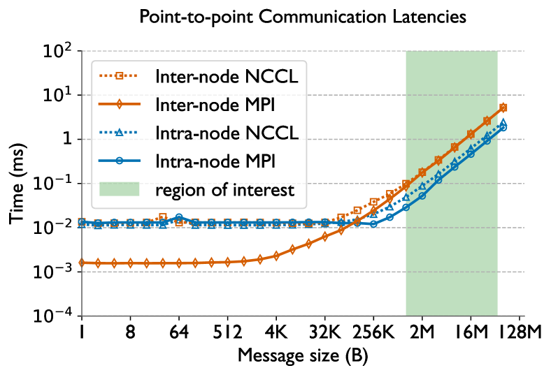
Figure 3: Execution time for point-to-point messages in MPI and NCCL on Summit using the OSU Micro-benchmarks v5.8 [18]. We use two GPUs on the same and different nodes for the intra- and inter-node experiments respectively.

We build our implementation of inter-layer parallelism on top of MPI4Py [19], a library which provides Python bindings for the MPI standard. We use MPI_Isend and MPI_Irecv to implement the Send and Receive methods mentioned in Algorithm 1. The MPI_Irecv s are issued preemptively at the beginning of a forward or backward pass to overlap the reception of the next message with the computation and thus achieve asynchronous messaging. In lines 13 and 21 of Algorithm 2, we have already shown how AxoNN is designed to support message driven scheduling for inter-layer parallelism. Combined with the asynchronous point-to-point communication backend discussed in this section, we are able to realize our goal of asynchronous message driven scheduling for improving hardware utilization.

IV-B Data parallel phase

We again had a choice between MPI and NCCL for the all-reduce operation in the data-parallel phase and we decided to make that choice based on empirical evidence. Figure 4 presents the performance of the all-reduce operation using MPI and NCCL. In this case, intra-node refers to performing the collective over all six GPUs of a single node and inter-node refers to performing it over 12 GPUs on two nodes. The results demonstrates the significantly better performance of NCCL (dashed lines) over MPI for collective communication. This makes NCCL the clear choice for AxoNN’s collective communication backend.

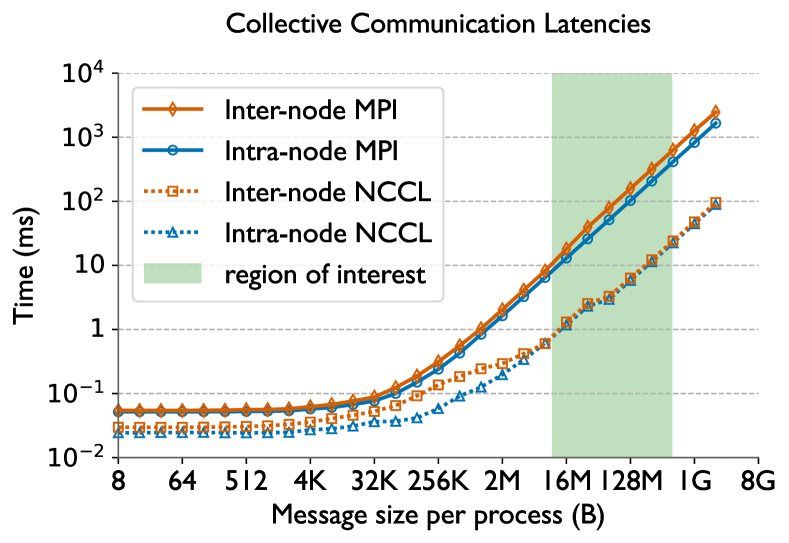
Figure 4: Execution time for an All-reduce operation in MPI and NCCL on Summit using the OSU Micro-benchmarks v5.8 [18]. We use six and twelve GPUs for the intra-node and inter-node experiments respectively.

Our implementation of data parallelism uses NCCL for the all-reduce operation over half-precision parameter gradients. We avoid using full-precision gradients to reduce communication times. To prevent overflow in the all-reduce operation, we pre-divide the loss by the total number of microbatches in the input batch. We use PyTorch’s torch.distributed API [10] for making NCCL all-reduce function calls.

V Memory and performance optimizations

In this section, we discuss optimizations that are critical to the memory utilization and performance of AxoNN. We implement these optimizations on top of the basic version of our framework discussed in Section IV. We verify their efficacy by conducting several experiments on a 12 billion parameter transformer neural network [11] on 48 NVIDIA V100 GPUs. Section VI-B provides the exact architectural hyperparameters of this model in Table I, and describes how these hyperparameters affect the computational and memory requirements of a transformer. For all the experiments in this section, the batch size and sequence length are fixed at 2048 and 512 respectively, and we use mixed-precision training [14] with the Adam optimizer [16].

V-A Memory optimizations for reducing activation memory

Gradient checkpointing reduces the amount of memory used to store activations by only storing the output activations of a subset of layers during the forward pass [20] . For a neural network with N layers $(l_{1},l_{2},..l_{N})$, this subset of layers is defined as $S_{\mathit{ckp}}=(l_{\mathit{ac}},l_{2\cdot\mathit{ac}},l_{3\cdot\mathit{ac}}....l_{N})$, where $\mathit{ac}$ is a tunable hyperparameter with the constraint that it should be a factor of N. Activations for layers that are not checkpointed are regenerated during their backward pass. For inter-layer parallelism, it can be shown that the maximum activation memory occupied per GPU with $\mathit{ac}$ as the gradient checkpointing hyperparameter is:

$$\mathrm{M_{activation}}\propto G_{\mathit{inter}}\times\left(\frac{N}{G_{\mathit{inter}}\times\mathit{ac}}\right)+1+ac$$ (1)

The value $\mathit{ac}=\sqrt{N}$ leads to the lowest value of $\mathrm{M_{activation}}$. We thus set the value of $ac$ to the factor of $\frac{N}{G_{\mathrm{inter}}}$ (the number of layers on each GPU) closest to $\sqrt{N}$. To the best of our knowledge, our work is the first to derive an optimal value of this hyperparameter for inter-layer parallelism. We implement gradient checkpointing using the torch.utils.checkpoint API provided by PyTorch [17].

V-B Memory optimizations for reducing $G_{\mathit{inter}}$ and improving performance of the inter-layer parallel phase

Narayanan et al. show empirically that the performance of inter-layer parallelism deteriorates with increasing values of ${G_{\mathit{inter}}}$ [5]. They attribute this to an increase in the idle time in the warmup phase with increasing ${G_{\mathit{inter}}}$. Below, we show analytically that it is not only the warmup phase, but the entire inter-layer parallel phase which suffers from inefficiency with increasing ${G_{\mathit{inter}}}$ by virtue of rising communication to computation ratios.

Lemma V.1

Given a neural network, batch size, and number of GPUs, the total amount of communication per GPU in the inter-layer parallel phase is proportional to $\mathit{G_{inter}}$.

Proof: The total amount of input data a GPU computes on reduces as the number of GPUs used for data parallelism increases. Hence, the amount of data per GPU is inversely proportional to $\mathit{G_{data}}$ given a fixed total number of GPUs that are split between data and inter-layer parallelism. It also follows that the amount of data computed on per GPU is directly proportional to $\mathit{G_{inter}}$. Assuming that the output activations of each layer of the neural network have the same size, the amount of point-to-point communication per GPU only depends on the amount of input data it consumes and not on the number of layers it houses. Thus the total amount of communication is directly proportional to $\mathit{G_{inter}}$.

Lemma V.2

Given a neural network, batch size, and number of GPUs, the total amount of computation per GPU in the inter-layer parallel phase is independent of $\mathit{G_{inter}}$.

Proof: We have shown in Lemma V.1 that the total amount of input data a GPU computes on is directly proportional to $\mathit{G_{inter}}$. Since layers are sharded evenly among the $\mathit{G_{inter}}$ GPUs of a row in Figure 2, the total amount of computation per instance of the input is inversely proportional to $\mathit{G_{inter}}$. Thus the total amount of computation per GPU is independent of $\mathit{G_{inter}}$.

Theorem V.3

Given a neural network, batch size, and number of GPUs, the ratio of the total amount of computation to communication in the inter-layer parallel phase is inversely proportional to $\mathit{G_{inter}}$.

Proof: Directly follows from Lemmas V.1 and V.2.

We thus expect the efficiency of inter-layer parallelism to decrease with increasing $\mathit{G_{inter}}$ due to an increase in the ratio of communication to computation. We empirically verify this phenomenon by studying the effect of varying $G_{\mathit{inter}}$ on performance. We gather the time spent in the inter-layer parallel phase for processing a batch of input using our reference transformer neural network for values of $G_{\mathit{inter}}=[6,12,24,48]$. The corresponding value of $G_{\mathit{data}}$ is automatically set to be $\frac{48}{G_{\mathit{inter}}}$. We fix the microbatch size and batch size to 1 and 2048 respectively. We also remove the optimizer states so that we do not run out of memory for lower values of $G_{\mathit{inter}}$. Figure 5 illustrates the results of our experiment. As expected, we observe significant gains in performance with decreasing $G_{\mathit{inter}}$.

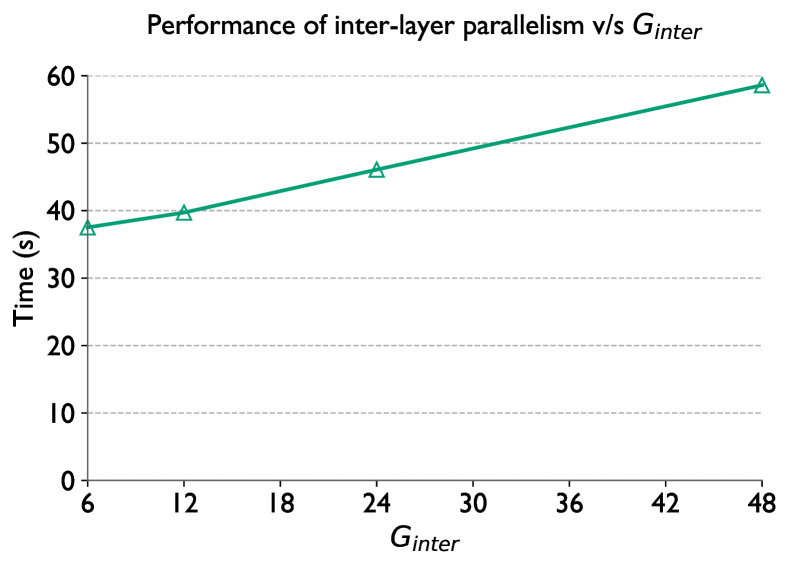
Figure 5: Time spent in the inter-layer parallel phase for a single batch for different values of ${G_{\mathit{inter}}}$ when training a 12 billion parameter transformer model on 48 GPUs of Summit.

Theorem V.3 thus provides a motivation to optimize the implementation by reducing the number of GPUs used for inter-layer parallelism. However, a smaller value of $G_{\mathit{inter}}$ requires the entire network to fit on a smaller number of GPUs, which increases the number of parameters per GPU. This increases the memory requirements per GPU. Lets say the number of parameters per GPU is $\phi=|\vec{\theta}|$ and we are using the Adam optimizer [16] which stores two state variables per parameter. The memory required to store model parameters, gradients and the optimizer states comes out to be $20\phi$ ($4\phi$ bytes each for $\vec{\theta}$ and $\nabla\vec{\theta}$, $2\phi$ bytes each for $\vec{\theta_{16}}$ and $\nabla\vec{\theta_{16}}$, and $8\phi$ bytes for $\vec{s_{opt}}$). Note that this analysis does not include memory required fori storing activations.

At $G_{\mathit{inter}}=6$ on our reference transformer, this would amount to 40 GB memory per GPU which is 2.5 times more than the 16 GB DRAM capacity of Summit’s V100 GPUs. To solve this problem, we introduce a novel memory optimization algorithm that reduces the amount of memory required to store the model parameters and optimizer states by five times.

Implementation: In our memory optimization, only the half precision model parameters ($\vec{\theta_{16}}$) and gradients ($\nabla\vec{\theta_{16}}$) reside on the GPU. Everything else is either moved to the CPU ($\vec{s_{opt}}$ and $\vec{\theta}$) or deleted entirely ($\nabla\vec{\theta}$) before the training begins. The training procedure requires $\vec{s_{opt}}$ and $\vec{\theta}$ on the GPU in the optimizer phase. We save memory by not fetching the entire $\vec{\theta}$ and $\vec{s_{opt}}$ arrays to the GPU, but only small equal sized chunks at a time. We call these chunks buckets and their size as the bucket-size ($\mathit{bsize}$). After fetching a bucket of $\vec{s_{opt}}$ and $\vec{\theta}$, we run the optimizer step on this data and offload it back to the CPU. GPU Memory is saved by reusing buffers across buckets.

The total memory footprint of the optimizer is only $16\mathit{bsize}$ now ($4\mathit{bsize}$ and $8\mathit{bsize}$ for the $\vec{\theta}$ and $\vec{s_{opt}}$ buckets respectively and another $4\mathit{bsize}$ for descaling the half precision gradients). With our memory optimizations, the total memory requirements to store model parameters and optimizier states is now $4\phi+16\mathit{bsize}$, down from $20\phi$. As $bsize\ll\phi$, this amounts to a 5$\times$ saving in memory utilization. Since the activation memory is unaffected the total memory saved should obviously be less than this number. With $G_{\mathit{inter}}=24$, $G_{\mathit{data}}=2$, microbatch size 1 and $bsize=16$ million our total memory usage for the reference transformer reduces four fold in practice - from 520 GB to 130.24 GB.

Next, we use our memory optimization algorithm with $bsize=16$ million to reduce $G_{\mathit{inter}}$ from 24 to 6, and study the performance implications. We expect an increase in the time it takes to complete the data parallel phase, because both the amount of data and number of GPUs participating in the all-reduce increases four fold. Figure 6 compares AxoNN’s performance with and without the memory optimizations. We notice an improvement of 13 percent in the absolute batch timings. While the time for the data parallel phase increases from 0.62s to 4.32s, the corresponding performance gain in the pipelining phase (46.08s v/s 34.05s) compensates for this increase. We expect higher speedups for larger values of batch size, which are typical in large scale model training.

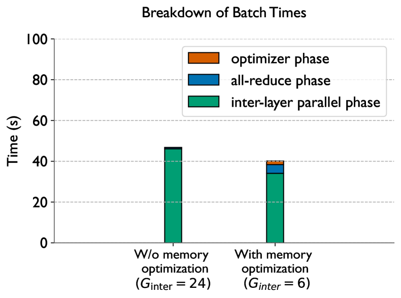
Figure 6: AxoNN’s performance for a single batch with and without our memory optimization on a 12 billion parameter transformer on 48 GPUs

V-C Overlapping all-reduce & optimizer phases for performance

After optimizing the inter-layer parallel phase, we turned our attention to the less time consuming all-reduce and optimizer phases. We observed that the all-reduce phase (in blue) takes 2.5 times longer than the optimizer phase (in green) (right bar in the Figure 6 plot). We hypothesize that by interleaving their executions, we could overlap data movement between the CPU and the GPU in the optimizer phase with the expensive collective communication of the data parallel phase. We explain our approach for enabling this overlap below.

Implementation: The main idea here is to issue the all-reduce call into smaller operations over chunks of the half precision gradients ($\nabla\vec{\theta_{16}}$). For convenience, we keep the size of the chunk as $k\times\mathit{bsize}$, where we call $k$ as the all-reduce coarsening factor. As soon as an all-reduce on a chunk finishes, we enqueue the optimizer step for the corresponding $k$ buckets and start the all-reduce of the next chunk. The key to achieving overlap is to use separate CUDA streams for the optimizer and the all-reduce. Figure 7 shows an Nvidia Nsight Sytems profile of our implementation.

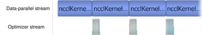
Figure 7: An Nsight profile of AxoNN training a 12 billion parameter transformer model on 48 GPUs shows the interleaving of the all-reduce and optimizer phases for a single batch. The two rows represent separate CUDA streams for the optimizer and all-reduce.

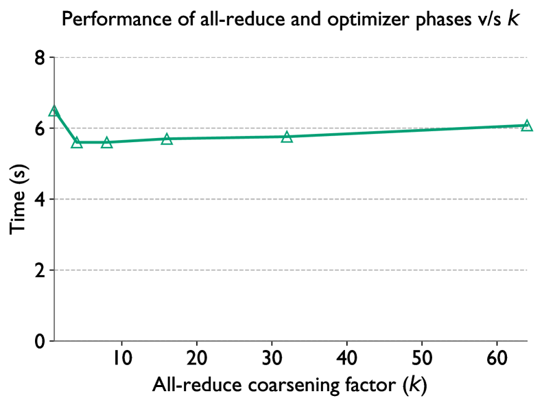
Figure 8: Combined execution time of optimizer and all-reduce phases for a single batch versus the coarsening factor, $k$, for the all-reduce.

We study the variation of the time it takes to finish the combined data parallel and optimizer phases with $k$ in Figure 8. At $k=1$, we observe high overheads due to too many all-reduce calls. Infact, performance is even worse than the case where we had no overlap between the two phases. We observe optimum behavior at two and four. Beyond that, we encounter increasing latencies since increasing $k$ makes the algorithm gravitate towards sequential behavior.

VI Experimental setup

This section provides an overview of our empirical evaluation of AxoNN against the current state-of-the-art frameworks in parallel deep learning. Along with comparing performance, we also verify the correctness of our implementation by training a neural network to completion and reporting the loss curves. We conduct all of our experiments on Oak Ridge National Laboratory’s Summit Cluster. Each node of Summit consists of two Power 9 CPUs each connected to 3 NVIDIA V100 GPUs via NVLink interconnects. The peak intra and inter-node bandwidth for GPU communication is 50 GB/s and 12.5 GB/s respectively. Each V100 GPU has 16 GB DRAM and a peak half precision throughput of 125 Tflop/s.

VI-A Choice of frameworks

We compare AxoNN with two frameworks implementing 3D parallelism (intra-layer, inter-layer, and data parallelism), namely - Megatron-LM [5] and DeepSpeed [6, 12], both of which have successfully demonstrated impressive performance when scaled to models with as many as trillion parameters. Both these frameworks augment Shoeybi et al.’s intra-layer parallelism [2] with a NCCL based implementation of inter-layer parallelism. Additionally, DeepSpeed uses the ZeRO [12] family of memory optimizations which distribute optimizer states across data parallel GPUs.

VI-B Choice of neural networks

We conduct our strong and weak scaling experiments on GPT-like [1, 3] transformer [11] neural networks on the task of causal language modeling. For a fair comparison, we use Megatron-LM’s extremely efficient implementation of the transformer kernel for all the three frameworks. A transformer can be parameterized by three hyperparameters - number of layers, hidden size, and number of attention heads. For more details about the transformer architecture, we refer the reader to Vaswani et al. [11]. We first verify the correctness of our implementation by training GPT-2 small [1] (110 million parameters)- to completion. Table I lists the transformer models and the corresponding GPU counts used in our weak scaling runs. We start with a 12 billion parameter transformer on 48 GPUs (8 nodes) and scale up to a 100 billion parameter transformer on 384 GPUs (64 nodes). We choose 48 GPUs as the starting point as it was the least number of GPUs the three frameworks could all train the 12 billion parameter transformer without running out of memory. For strong scaling, we choose the 12 billion parameter transformer from Table I and vary the number of GPUs from 48 to 384.

TABLE I: Details about the transformers models used in the weak scaling study

		Parameters		Hidden	Attention
Nodes	GPUs	(in Billions)	Layers	Dimension	Heads
8	48	12	48	4512	24
16	96	24	48	6336	36
32	192	50	96	6528	48
64	384	100	96	9360	60

VI-C Dataset and hyperparameters

The batch size and number of parameters are the two most important quantities that affect hardware performance. We thus perform two separate experiments that vary the batch size and number of parameters independently with increasing GPU counts. Since the dataset size is fixed, both these experiments neatly translate to a strong scaling and weak scaling setup. We note that it is absolutely imperative not to vary both these quantities together, otherwise they can artificially inflate performance numbers. Thus we fix the batch size for the weak scaling run at 16384. For the strong scaling experiments, we vary the batch size linearly, starting with 4096 for 48 GPUs (8 nodes) and scaling upto 32768 for 384 GPUs (48 nodes). We train all our models on the wikitext-103 [21] dataset which consists of around 100 million English words sourced from more than 28000 Wikipedia articles. We fix the sequence length and vocabulary size at 512 and 51200 respectively. We use the Adam optimizer [16] with learning rate 0.001, $\beta_{1}=0.9$, $\beta_{2}=0.999$ and 0.01 as the decoupled weight decay regularization [22] coefficient. We tune $G_{\mathit{inter}}$, $G_{\mathit{intra}}$, and $G_{\mathit{data}}$ for Megatron-LM and DeepSpeed. For AxoNN we just tune $G_{\mathit{inter}}$ and $G_{\mathit{data}}$ since it does not implement intra-layer parallelism. For AxoNN’s memory optimizations we fix $bsize$ to 4 million and $k$ to 4.

VI-D Metrics

We use two metrics in our experiments - namely expected training time and the percentage of peak half precision throughput. Both of these are metrics derived from the average batch time, which we calculate by training for eleven batches and averaging the timings of the last ten. In accordance with the training regime employed for GPT-3 [3], we define the expected training time as the total time it would take to train a transformer on a total of 300 billion tokens. Let $b$, $s$, $l$, $h$, $V$, $t$ be the batch size, sequence length, number of layers, hidden size, vocabulary size, and the average batch time respectively. Then the estimated training time can be estimated from the batch time as follows:

$$\mathit{estimated\_training\_time}=3e10^{11}\frac{t}{bs}$$ (2)

We derive the average flop/s by using Narayanan et al.’s lower bound for flops in a batch for a transformer [5]:

$$\mathit{flop/s}=\frac{96bslh^{2}}{t}(1+\frac{s}{6h}+\frac{V}{16lh})$$ (3)

Dividing this by the total peak half precision throughput of all the GPUs used for training (on Summit this is 125 Tflop/s per GPU) yields the percentage of peak throughput.

VII Results

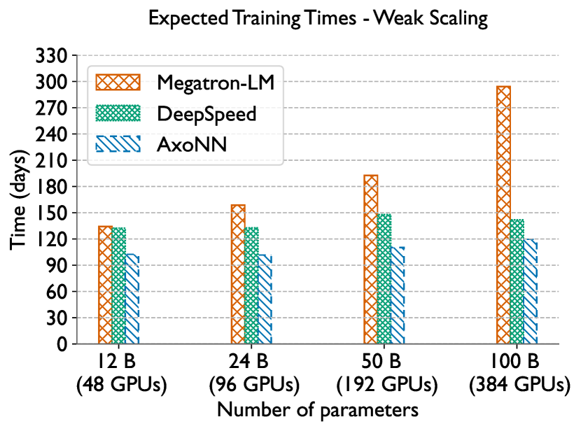
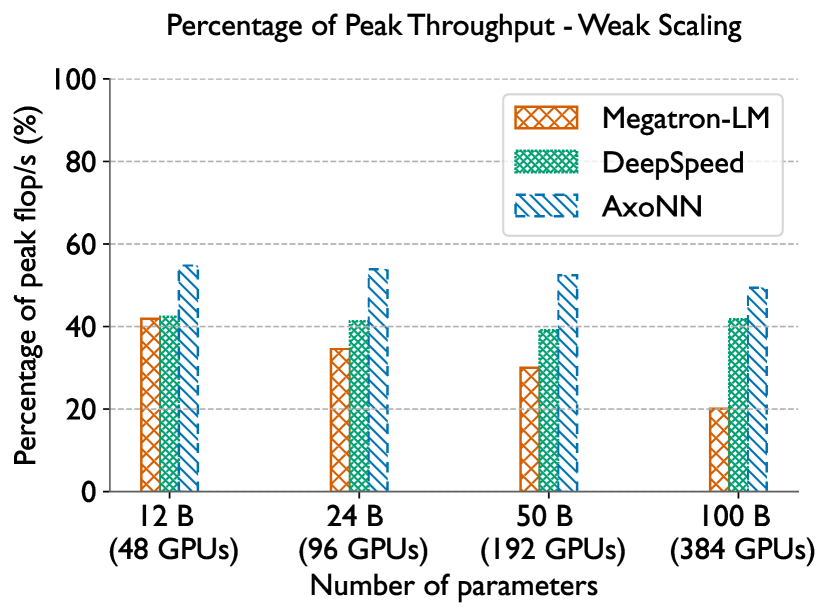
Figure 9: Plots comparing the weak scaling performance of AxoNN with other frameworks: expected training times (left) and % of peak GPU throughput (right).

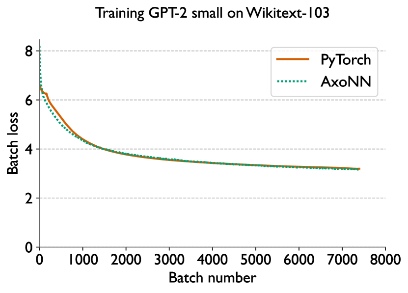
Figure 10: Loss curves for training GPT-2 small on the wikitext-103 dataset. We run AxoNN on 12 GPUs ($G_{\mathit{inter}}=2$) and PyTorch on a single GPU.

We now present the results of the experiments outlined in the previous section.

VII-A Training validation

It is critical to ensure that parallelizing the training process does not adversely impact its convergence. Diverging training loss curves are a sign of undetected bugs in the implementation or statistical inefficiency of the parallel algorithm. To validate the accuracy of our parallel implementation, we train the 110 million parameter GPT-2 small to completion using PyTorch on a single GPU and using AxoNN on 12 GPUs with $G_{\mathit{inter}}=2$. Figure 10 shows the training loss for PyTorch, and AxoNN and we can see that the loss curves are identical. This validates our AxoNN implementation.

VII-B Weak scaling performance

To be fair to each framework, we tune various hyperparameters for each framework on each GPU count and use the best values for reporting performance results. Table II lists the optimal hyperparameters we obtain in our tuning experiments for each framework in the weak scaling experiment. Across all model sizes, AxoNN uses four to eight times the number of GPUs for data parallelism as compared to Megatron-LM. This number is identical for AxoNN and DeepSpeed for the 12 billion and 24 billion parameter models but for the larger 50 and 100 billion parameter models, AxoNN uses twice as many GPUs for data parallelism as DeepSpeed. Since data parallelism is embarrassingly parallel, this ends up substantially improving AxoNN’s performance.

TABLE II: Optimal hyperparameter values obtained from tuning experiments for the weak scaling studies.

No. of Params. (billions)	Framework	Micro Batch Size	$G_{\mathit{intra}}$	$G_{\mathit{inter}}$	$G_{\mathit{data}}$
12	AxoNN	8	-	6	8
	DeepSpeed	2	3	2	8
	Megatron-LM	8	3	16	1
24	AxoNN	4	-	12	8
	DeepSpeed	2	3	4	8
	Megatron-LM	1	3	16	2
50	AxoNN	4	-	24	8
	DeepSpeed	1	3	16	4
	Megatron-LM	8	6	32	1
100	AxoNN	2	-	48	8
	DeepSpeed	1	3	32	4
	Megatron-LM	4	12	32	1

Figure 9 (left) presents a performance comparison of the three frameworks in the weak scaling experiment. When compared with the next best framework - DeepSpeed, AxoNN decreases the estimated training time by over a month for the 12, 24 and 50 billion parameter models and 22 days for the 100 billion parameter model. For the 100 billion parameter model, AxoNN is faster than DeepSpeed by 1.18$\times$ and Megatron-LM by 2.46$\times$! This is significant for deep learning research as it allows us to train larger models faster. Even at identical values of $G_{\mathit{data}}$ for the 12 and 24 billion parameter models, AxoNN surpasses DeepSpeed because of our asynchronous, message-driven implementation of inter-layer parallelism. These results suggest that AxoNN could scale to training trillion parameter neural networks on thousands of GPUs in the future. AxoNN also delivers an impressive 49-54% of peak half precision throughput on Summit GPUs, outperforming DeepSpeed (39-42%) and Megatron-LM (21-41%) (see Figure 9, right).

VII-C Strong scaling performance

As with weak scaling, we first tuned hyperparameters for each framework for strong scaling experiments. For these experiments we see all the three frameworks using the same values of $G_{\mathit{inter}}$, $G_{\mathit{intra}}$ (not applicable for AxoNN) as Table II and scale the value of $G_{data}$ with increasing GPU counts. This is a testament to data parallelism’s near perfect scaling behavior due to its embarrassingly parallel nature. Figure 11 compares the strong scaling performance of the three frameworks. Once again, AxoNN again outperforms both DeepSpeed and Megatron-LM by 11.47 and 18.14% respectively on 384 GPUs.

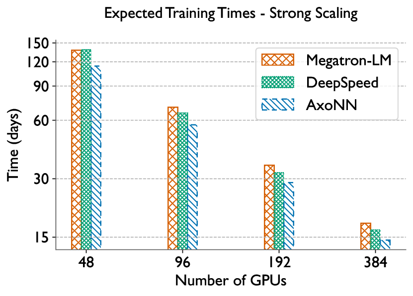
Figure 11: Plots comparing the strong scaling performance of AxoNN with other frameworks: training times for the 12 billion parameter transformer model.

VIII Related work

Due to it’s simplicity and embarrassingly parallel nature, data parallelism has been the most commonly adopted algorithm in parallel deep learning research. Initial frameworks gravitated towards asynchronous data parallelism with parameter servers [23, 24]. Chen et al however established that asynchronous data parallelism does not work on a large number of GPUs [25]. The ensuing discrepancy between model weights on each GPU ends up hurting the rate of convergence. Subsequently, modern implementations of data parallelism are synchronous and do not employ central parameter servers [10, 26, 2, 5, 12, 15]. These frameworks average gradients using all-reduce communication primitives in a bulk synchronous fashion after the backward pass of a batch is completed. With advances in interconnect technology and communication libraries [8], the cost of synchronous all-reduce communication has drastically reduced, making data parallelism the most effective algorithm for scaling neural network training on 100s of GPUs.

Data parallelism needs to be combined with one or both of intra-layer and inter-layer parallelism when the memory requirements of a neural network exceed the DRAM capacity of a GPU. The exponentially increasing parameter sizes of modern neural networks [1, 3] have made it absolutely critical to develop efficient algorithms for intra-layer and inter-layer parallelism. While a number of frameworks have been proposed for intra-layer parallelism [4, 2], frequent collective communication calls after the computation of each layer prevents them from scaling beyond a small number of GPUs connected by NVLink. Algorithms for inter-layer parallelism fall into two categories based on the type of pipelining they implement: namely pipelining with flushing [27, 5, 6, 28] or pipelining without flushing [7, 29]. Under the former approach, worker GPUs update their weights only after all of the microbatches of a batch have been flushed out of the pipeline. While this maintains strict optimizer semantics, constant flushing leads to inefficient hardware utilization. This problem is greatly exacerbated at higher GPU counts. Pipelining without flushing was proposed as a remedy for this problem. In this approach a constant number of microbatches are always present in the pipeline. Each GPU updates their weights asynchronously after completing the backward pass of a microbatch. While this leads to increased hardware utilization, the departure from exact optimizer semantics ends up hurting model convergence severely. Again, greater the GPU count the more severe this problem is. Subsequently, modern parallel deep learning frameworks have adopted pipelining with flushing for realizing inter-layer parallelism.

To counteract the extreme memory requirements of modern neural networks, Rajbhandari et al. have augmented data parallelism with a number of memory optimizations (ZeRO [12], ZeRO-Offload [30], ZeRO-Infinity [15]). ZeRO distributes optimizer states, parameters and gradients across data-parallel GPUs. ZeRO-Offload and ZeRO-Infinity are targeted towards extremely memory scarce environments. To reduce GPU memory utilization they offload data to the CPU or NVMe.

IX Conclusion

In this work, we presented a new highly scalable parallel framework for deep learning, called AxoNN. We have demonstrated that AxoNN utilizes available hardware resources efficiently by exploiting asynchrony and message-driven scheduling. We augmented AxoNN with a novel memory optimization algorithm that not only provided a four-fold savings in GPU memory utilization, but also boosted performance by over 13%. In both strong and weak scaling experiments, AxoNN outperformed the state-of-the-art for training large multi-billion parameter transformer models. We believe that AxoNN will allow deep learning researchers to save valuable resources and time in their training runs. Our results give us hope that we can use AxoNN to train transformer models with more than one trillion parameters on thousands of GPUs. We plan to open-source the weights of these trained models for the benefit of the research community.

References

- [1] A. Radford, J. Wu, R. Child, D. Luan, D. Amodei, and I. Sutskever, “Language models are unsupervised multitask learners,” 2019.
- [2] M. Shoeybi, M. Patwary, R. Puri, P. LeGresley, J. Casper, and B. Catanzaro, “Megatron-lm: Training multi-billion parameter language models using model parallelism,” 2020.
- [3] T. B. Brown, B. Mann, N. Ryder, M. Subbiah, J. Kaplan, P. Dhariwal, A. Neelakantan, P. Shyam, G. Sastry, A. Askell, S. Agarwal, A. Herbert-Voss, G. Krueger, T. Henighan, R. Child, A. Ramesh, D. M. Ziegler, J. Wu, C. Winter, C. Hesse, M. Chen, E. Sigler, M. Litwin, S. Gray, B. Chess, J. Clark, C. Berner, S. McCandlish, A. Radford, I. Sutskever, and D. Amodei, “Language models are few-shot learners,” CoRR, vol. abs/2005.14165, 2020. [Online]. Available: https://arxiv.org/abs/2005.14165
- [4] N. Shazeer, Y. Cheng, N. Parmar, D. Tran, A. Vaswani, P. Koanantakool, P. Hawkins, H. Lee, M. Hong, C. Young, R. Sepassi, and B. Hechtman, “Mesh-tensorflow: Deep learning for supercomputers,” in Advances in Neural Information Processing Systems, S. Bengio, H. Wallach, H. Larochelle, K. Grauman, N. Cesa-Bianchi, and R. Garnett, Eds., vol. 31. Curran Associates, Inc., 2018. [Online]. Available: https://proceedings.neurips.cc/paper/2018/file/3a37abdeefe1dab1b30f7c5c7e581b93-Paper.pdf
- [5] D. Narayanan, M. Shoeybi, J. Casper, P. LeGresley, M. Patwary, V. Korthikanti, D. Vainbrand, P. Kashinkunti, J. Bernauer, B. Catanzaro, A. Phanishayee, and M. Zaharia, “Efficient large-scale language model training on GPU clusters,” CoRR, vol. abs/2104.04473, 2021. [Online]. Available: https://arxiv.org/abs/2104.04473
- [6] Microsoft, “3d parallelism with megatronlm and zero redundancy optimizer,” https://github.com/microsoft/DeepSpeedExamples/tree/master/Megatron-LM-v1.1.5-3D_parallelism, 2021.
- [7] D. Narayanan, A. Harlap, A. Phanishayee, V. Seshadri, N. Devanur, G. Granger, P. Gibbons, and M. Zaharia, “Pipedream: Generalized pipeline parallelism for dnn training,” in ACM Symposium on Operating Systems Principles (SOSP 2019), October 2019. [Online]. Available: https://www.microsoft.com/en-us/research/publication/pipedream-generalized-pipeline-parallelism-for-dnn-training/
- [8] NVIDIA, “Nccl,” https://docs.nvidia.com/deeplearning/nccl/user-guide/docs/overview.html.
- [9] Facebook, “Gloo,” https://github.com/facebookincubator/gloo.
- [10] S. Li, Y. Zhao, R. Varma, O. Salpekar, P. Noordhuis, T. Li, A. Paszke, J. Smith, B. Vaughan, P. Damania, and S. Chintala, “Pytorch distributed: Experiences on accelerating data parallel training,” Proc. VLDB Endow., vol. 13, no. 12, p. 3005–3018, Aug. 2020. [Online]. Available: https://doi.org/10.14778/3415478.3415530
- [11] A. Vaswani, N. Shazeer, N. Parmar, J. Uszkoreit, L. Jones, A. N. Gomez, L. Kaiser, and I. Polosukhin, “Attention is all you need,” CoRR, vol. abs/1706.03762, 2017. [Online]. Available: http://arxiv.org/abs/1706.03762
- [12] S. Rajbhandari, J. Rasley, O. Ruwase, and Y. He, “Zero: Memory optimizations toward training trillion parameter models,” in Proceedings of the International Conference for High Performance Computing, Networking, Storage and Analysis, ser. SC ’20. IEEE Press, 2020.
- [13] D. E. Rumelhart, G. E. Hinton, and R. J. Williams, “Learning Representations by Back-propagating Errors,” Nature, vol. 323, no. 6088, pp. 533–536, 1986. [Online]. Available: http://www.nature.com/articles/323533a0
- [14] P. Micikevicius, S. Narang, J. Alben, G. Diamos, E. Elsen, D. Garcia, B. Ginsburg, M. Houston, O. Kuchaiev, G. Venkatesh, and H. Wu, “Mixed precision training,” in International Conference on Learning Representations, 2018. [Online]. Available: https://openreview.net/forum?id=r1gs9JgRZ
- [15] S. Rajbhandari, O. Ruwase, J. Rasley, S. Smith, and Y. He, “Zero-infinity: Breaking the gpu memory wall for extreme scale deep learning,” ser. SC ’21. New York, NY, USA: Association for Computing Machinery, 2021. [Online]. Available: https://doi.org/10.1145/3458817.3476205
- [16] D. P. Kingma and J. Ba, “Adam: A method for stochastic optimization,” in 3rd International Conference on Learning Representations, ICLR 2015, San Diego, CA, USA, May 7-9, 2015, Conference Track Proceedings, Y. Bengio and Y. LeCun, Eds., 2015. [Online]. Available: http://arxiv.org/abs/1412.6980
- [17] A. Paszke, S. Gross, F. Massa, A. Lerer, J. Bradbury, G. Chanan, T. Killeen, Z. Lin, N. Gimelshein, L. Antiga, A. Desmaison, A. Kopf, E. Yang, Z. DeVito, M. Raison, A. Tejani, S. Chilamkurthy, B. Steiner, L. Fang, J. Bai, and S. Chintala, “Pytorch: An imperative style, high-performance deep learning library,” in Advances in Neural Information Processing Systems, H. Wallach, H. Larochelle, A. Beygelzimer, F. d'Alché-Buc, E. Fox, and R. Garnett, Eds., vol. 32. Curran Associates, Inc., 2019. [Online]. Available: https://proceedings.neurips.cc/paper/2019/file/bdbca288fee7f92f2bfa9f7012727740-Paper.pdf
- [18] O. S. University, “Osu micro-benchmarks 5.8,” http://mvapich.cse.ohio-state.edu/benchmarks/.
- [19] L. Dalcin and Y.-L. L. Fang, “mpi4py: Status update after 12 years of development,” Computing in Science Engineering, vol. 23, no. 4, pp. 47–54, 2021.
- [20] T. Chen, B. Xu, C. Zhang, and C. Guestrin, “Training deep nets with sublinear memory cost,” 2016.
- [21] S. Merity, C. Xiong, J. Bradbury, and R. Socher, “Pointer sentinel mixture models,” CoRR, vol. abs/1609.07843, 2016. [Online]. Available: http://arxiv.org/abs/1609.07843
- [22] I. Loshchilov and F. Hutter, “Fixing weight decay regularization in adam,” CoRR, vol. abs/1711.05101, 2017. [Online]. Available: http://arxiv.org/abs/1711.05101
- [23] T. Chilimbi, Y. Suzue, J. Apacible, and K. Kalyanaraman, “Project adam: Building an efficient and scalable deep learning training system,” in 11th USENIX Symposium on Operating Systems Design and Implementation (OSDI 14). Broomfield, CO: USENIX Association, Oct. 2014, pp. 571–582. [Online]. Available: https://www.usenix.org/conference/osdi14/technical-sessions/presentation/chilimbi
- [24] J. Dean, G. S. Corrado, R. Monga, K. Chen, M. Devin, Q. V. Le, M. Z. Mao, M. Ranzato, A. Senior, P. Tucker, K. Yang, and A. Y. Ng, “Large scale distributed deep networks,” in NIPS, 2012.
- [25] J. Chen, R. Monga, S. Bengio, and R. Jozefowicz, “Revisiting distributed synchronous sgd,” in International Conference on Learning Representations Workshop Track, 2016. [Online]. Available: https://arxiv.org/abs/1604.00981
- [26] A. Sergeev and M. D. Balso, “Horovod: fast and easy distributed deep learning in tensorflow,” 2018.
- [27] Y. Huang, Y. Cheng, A. Bapna, O. Firat, D. Chen, M. Chen, H. Lee, J. Ngiam, Q. V. Le, Y. Wu, and z. Chen, “Gpipe: Efficient training of giant neural networks using pipeline parallelism,” in Advances in Neural Information Processing Systems, H. Wallach, H. Larochelle, A. Beygelzimer, F. d'Alché-Buc, E. Fox, and R. Garnett, Eds., vol. 32. Curran Associates, Inc., 2019. [Online]. Available: https://proceedings.neurips.cc/paper/2019/file/093f65e080a295f8076b1c5722a46aa2-Paper.pdf
- [28] M. Tanaka, K. Taura, T. Hanawa, and K. Torisawa, “Automatic graph partitioning for very large-scale deep learning,” in 35th IEEE International Parallel and Distributed Processing Symposium, IPDPS 2021, Portland, OR, USA, May 17-21, 2021. IEEE, 2021, pp. 1004–1013. [Online]. Available: https://doi.org/10.1109/IPDPS49936.2021.00109
- [29] B. Yang, J. Zhang, J. Li, C. Re, C. Aberger, and C. De Sa, “Pipemare: Asynchronous pipeline parallel dnn training,” in Proceedings of Machine Learning and Systems, A. Smola, A. Dimakis, and I. Stoica, Eds., vol. 3, 2021, pp. 269–296. [Online]. Available: https://proceedings.mlsys.org/paper/2021/file/6c8349cc7260ae62e3b1396831a8398f-Paper.pdf
- [30] J. Ren, S. Rajbhandari, R. Y. Aminabadi, O. Ruwase, S. Yang, M. Zhang, D. Li, and Y. He, “Zero-offload: Democratizing billion-scale model training,” CoRR, vol. abs/2101.06840, 2021. [Online]. Available: https://arxiv.org/abs/2101.06840