Neural Relightable Participating Media Rendering

Abstract

Learning neural radiance fields of a scene has recently allowed realistic novel view synthesis of the scene, but they are limited to synthesize images under the original fixed lighting condition. Therefore, they are not flexible for the eagerly desired tasks like relighting, scene editing and scene composition. To tackle this problem, several recent methods propose to disentangle reflectance and illumination from the radiance field. These methods can cope with solid objects with opaque surfaces but participating media are neglected. Also, they take into account only direct illumination or at most one-bounce indirect illumination, thus suffer from energy loss due to ignoring the high-order indirect illumination. We propose to learn neural representations for participating media with a complete simulation of global illumination. We estimate direct illumination via ray tracing and compute indirect illumination with spherical harmonics. Our approach avoids computing the lengthy indirect bounces and does not suffer from energy loss. Our experiments on multiple scenes show that our approach achieves superior visual quality and numerical performance compared to state-of-the-art methods, and it can generalize to deal with solid objects with opaque surfaces as well.

1 Introduction

From natural phenomenons like fog and cloud to ornaments like jade artworks and wax figures, participating media objects are pervasive in both real life and virtual content like movies or games. Inferring the bounding geometry and scattering properties of participating media objects from observed images is a long-standing problem in both computer vision and graphics. Traditional methods addressed the problem by exploiting specialized structured lighting patterns [1, 2, 3] or using discrete representations [4]. These methods, however, require the bounding geometry of participating media objects to be known.

Learning neural radiance fields or neural scene representations [5, 6, 7] has achieved remarkable progress in image synthesis. They are able to optimize the representations with the assistance of a differentiable ray marching process. However, these methods are mostly designed for novel view synthesis and have baked in materials and lighting into the radiance fields or surface color. Therefore, they can hardly support downstream tasks such as relighting and scene editing. Recent work [8, 9] has taken initial steps to disentangle the lighting and materials from radiance. For material, their methods are primarily designed for solid objects with opaque surfaces, thus they assume an underlying surface at each point with a normal and a BRDF. The assumed prior, however, does not apply to non-opaque participating media which has no internal surfaces. For lighting, neural reflectance field [8] simulates direct illumination from a single point light, whereas NeRV [9] handles direct illumination and one-bounce indirect illumination. They generally suffer from the energy loss issue due to ignoring the high-order indirect illumination. However, indirect lighting from multiple scattering plays a significant role in the final appearance [10] of participating media.

In this paper, we propose a novel neural representation for learning relightable participating media. Our method takes as input a set of posed images with varying but known lighting conditions and designs neural networks to learn a disentangled representation for the participating media with physical properties, including volume density, scattering albedo and phase function parameter. To synthesize images, we embed a differentiable physically-based ray marching process in the framework. In addition, we propose to simulate global illumination by embedding the single scattering and multiple scattering estimation into the ray marching process, where single scattering is simulated by Monte Carlo ray tracing and the incident radiance from multiple scattering is approximated by spherical harmonics (SH). Without supervising with ground-truth lighting decomposition, our method is able to learn a decomposition of direct lighting and indirect lighting in an unsupervised manner.

Our comprehensive experiments demonstrate that our method achieves better visual quality and higher numerical performance compared to state-of-the-art methods. Meanwhile, our method can generalize to handle solid objects with opaque surfaces. We also demonstrate that our learned neural representations of participating media allow relighting, scene editing and insertion into another virtual environment. To summarize, our approach has the following contributions:

1. We propose a novel method to learn a disentangled neural representation for participating media from posed images and it is able to generalize to solid objects.

2. Our method deals with both single scattering and multiple scattering and enables the unsupervised decomposition of direct illumination and indirect illumination.

3. We demonstrate flexibility of the learned representation of participating media for relighting, scene editing and scene compositions.

2 Related Work

Neural scene representations.

Neural scene representations [11, 7, 6] are important building blocks for the recent progress in synthesizing realistic images. Different from representations of components such as ambient lighting and cameras [12, 13, 14] of scenes, neural scene representation [11] learns an embedding manifold from 2D images and scene representation networks [7] aim to infer the 3D context of scenes from images. Classic explicit 3D representations, such as voxels [15, 16, 6], multiplane images [17, 18] and proxy geometry [19] are exploited to learn neural representations for specific purposes. These explicit representations generally suffer from the intrinsic resolution limitation. To sidestep the limitation, most recent approaches shift towards implicit representations, like signed distance fields [20, 21], volumetric occupancy fields [22, 23, 24, 25], or coordinate-based neural networks [26, 7, 27, 28]. By embedding a differentiable rendering process like ray marching [6, 5] or sphere tracing [7, 29] into these implicit representations, these methods are capable of optimizing the scene representations from observed images and synthesizing novel views after training. While they generally show improved quality compared to interpolation based novel view synthesis methods [30, 31], the learned representations are usually texture colors and radiance, without separating lighting and materials. By contrast, we propose to learn a neural representation with disentangled volume density, scattering properties and lighting, which allow the usages in relighting, editing and scene composition tasks.

Volume geometry and properties capture.

Acquiring geometry and scattering properties of participating media has long been of the interest to the computer vision and graphics community. Early methods utilize sophisticated scanning and recording devices [32, 2] and specialized lighting patterns [3, 1] to capture volume density. Computational imaging methods [33, 34] frame the inference of scattering properties from images as an inverse problem, but they require that the geometries of objects are known. Based on the differentiable path tracing formulation [35], the inverse transport method [36] incorporates a differentiable light transport [37] module within an analysis-by-synthesis pipeline to infer scattering properties, but it aims for known geometries and homogeneous participating media. In contrast, our method learns the geometries and scattering properties of participating media simultaneously and our method can deal with both homogeneous and heterogeneous participating media.

Relighting.

Neural Radiance Field (NeRF) [5] and its later extensions [38] encode the geometry and radiance into MLPs and leverage ray marching to synthesize new views. While they achieve realistic results, they are limited to synthesize views under the same lighting conditions as in training. To mitigate this, appearance latent code [39, 40] are used to condition on the view synthesis. Recent approaches [8, 9] decompose materials and lighting by assuming an opaque surface at each point, but this does not apply to participating media. After training, density and materials can be extracted [41] to render new views using Monte Carlo methods [42, 43, 44]. Instead, our method models participating media as a field of particles that scatter and absorb light, which are in accordance with its nature. Neural reflectance field [45, 8] requires collocated cameras and lights during training and simulates only direct illumination. NeRV [9] and OSF [46] simulate merely one-bounce indirect light transport because of the prohibitive computation cost for long paths. However, ignoring the high-order indirect illumination leads to the potential problem of energy loss. By contrast, we use Monte Carlo ray tracing to compute direct lighting and propose to learn a spherical harmonic field for estimating the complete indirect lighting. The PlenOctree [47] uses spherical harmonics to represent the outgoing radiance field as in NeRF, but it does not allow relighting. With both direct illumination and indirect illumination properly estimated, our method enables a principled disentanglement of volume density, scattering properties, and lighting.

3 Background

Volume rendering.

The radiance carried by a ray after its interaction with participating media can be computed based on the radiative transfer equation [48]

$$L_{o}\left(\bm{r}_{0},\bm{r}_{d}\right)=\int_{0}^{\infty}\tau\left(\bm{r}(t)\right)\sigma\left(\bm{r}(t)\right)L\left(\bm{r}(t),-\bm{r}_{d}\right)\mathop{}\!\mathrm{d}t.$$ (1)

Here, $\bm{r}$ is a ray starting from $\bm{r}_{0}$ along the direction $\bm{r}_{d}$ and $\bm{r}(t)=\bm{r}_{o}+t\cdot{r}_{d}$ denotes a point along the ray at the parametric distance $t$. $L_{o}$ is the received radiance at $\bm{r}_{0}$ along $\bm{r}_{d}$. $\sigma$ denotes the extinction coefficient that is referred to as volume density. The $\tau\left(\bm{r}(t)\right)$ is the transmittance between $\bm{r}(t)$ and $\bm{r}_{0}$ and it can be computed by $\exp\left(-\int_{0}^{t}\sigma(\bm{r}(s))\mathop{}\!\mathrm{d}s\right)$. The $L(\cdot)$ inside the integral stands for the in-scattered radiance towards $\bm{r}_{0}$ along $-\bm{r}_{d}$. NeRF [5] models the in-scattered radiance $L$ (Eq. 1) as a view dependent color $c$, but it ignores the underlying scattering event and incident illumination. Since the learned radiance field of NeRF bakes in the lighting and materials, it allows merely view synthesis under the original fixed lighting, without the support for relighting.

Ray marching.

The integral in Equation 1 can be solved with the numerical integration method, ray marching [49]. This is generally done by casting rays into the volume and taking point samples along each ray to collect volume density and color values [5, 6]. The predicted color of a ray is computed by $L_{o}\left(\bm{r}_{0},\bm{r}_{d}\right)=\sum_{j}\tau_{j}\cdot\alpha_{j}\cdot L\left(\bm{r}(t_{j}),-\bm{r}_{d}\right)$, where $\alpha_{j}=1-\exp\left(-\sigma_{j}\cdot\delta_{j}\right)$, $\delta_{j}=\|t_{j+1}-t_{j}\|_{2}$ and $\tau_{j}=\prod_{i=1}^{j-1}(1-\alpha_{i})$.

4 Neural Relightable Participating Media

In this work, we aim to learn neural representations of participating media with disentangled volume density and scattering properties. We model the participating media as a field of particles that absorb and scatter light-carrying rays. Below we first describe our disentangled neural representation based on a decomposition with single scattering and multiple scattering. Then, we depict our neural network design, followed by details of a volume rendering process for synthesizing images and the details of training.

4.1 Lighting Decomposition

We firstly write the in-scattered radiance $L\left(\bm{r}(t),-\bm{r}_{d}\right)$ in Equation 1 as an integral of light-carrying spherical directions over a $4\pi$ steradian range

$$L\left(\bm{r}(t),-\bm{r}_{d}\right)=\int_{\Omega_{4\pi}}S\left(\bm{r}(t),-\bm{r}_{d},\omega_{i}\right)L_{in}(\bm{r}(t),\omega_{i})\mathop{}\!\mathrm{d}\omega_{i},$$ (2)

where $L_{in}$ is the incident radiance at $\bm{r}(t)$ from the direction $\omega_{i}$. $S(\cdot)$ is a scattering function which determines the portion of lighting that is deflected towards the $-\bm{r}_{d}$. Previous methods [8, 9, 41] assume a surface prior with a normal at every point and account for $2\pi$ hemispherical incident directions. Accordingly, they define the scattering function $S$ as a BRDF function. This assumption, however, can hardly match the participating media objects which have no internal surfaces and normals. By contrast, we deal with light-carrying directions over the full $4\pi$ steradian range. Specifically, we define $S=a(\bm{r}(t))\cdot\rho(-\bm{r}_{d},\omega_{i},g)$ to account for the scattering over the full spherical directions. Here, $a(\bm{r}(t))$ is the scattering albedo. $\rho$ is the Henyey-Greenstein (HG) [50] phase function that decides the scattering directionality (Appendix A), where $g$ is an asymmetry parameter in $(-1,1)$. For brevity, we omit $g$ in the notation of $\rho$. Then, we can rewrite the radiance of ray $\bm{r}$ as the disentangled form:

$$L_{o}\left(\bm{r}_{0},\bm{r}_{d}\right)=\int_{0}^{\infty}\tau\left(\bm{r}(t)\right)\sigma\left(\bm{r}(t)\right)\int_{\Omega_{4\pi}}a(\bm{r}(t))\rho(-\bm{r}_{d},\omega_{i})L_{in}(\bm{r}(t),\omega_{i})\mathop{}\!\mathrm{d}\omega_{i}\mathop{}\!\mathrm{d}t,$$ (3)

from which the volume density $\sigma$ decides the geometries, and the albedo $a$ along with the phase function $\rho$ controls the scattering of rays. We propose to train neural networks to learn the volume density and scattering properties.

To compute $L_{o}$, we additionally need to estimate $L_{in}$ (Eq. 3). This can be conducted by recursively substituting the $L_{o}$ into $L_{in}$ and expressing the radiance for a pixel $k$ as an integral over all paths $P_{k}=\int_{\Psi}g_{k}(\bar{x})d\mu(\bar{x})$, where $\bar{x}$ is a light-carrying path, $g_{k}$ denotes a measurement contribution function, $\mu$ is the measure for the path space, and $\Psi$ is the space of paths with all possible lengths. $P_{k}$ is then computed by a summation of the contributions of all paths. The contribution of a path with length $i$ can be written as

$$P_{k,i}=\int_{l_{1}}\int_{\Omega}\cdots\int_{l_{i-1}}\int_{\Omega}L_{e}\left(x(t_{i-1})\right)V\left(x(t_{i-1}),\omega_{i-1}\right)\mathcal{T}(P_{k,i})\mathop{}\!\mathrm{d}t_{1}\mathop{}\!\mathrm{d}\omega_{1}\cdots\mathop{}\!\mathrm{d}t_{i-1}\mathop{}\!\mathrm{d}\omega_{i-1},$$ (4)

where $x(t_{i-1})$ is a point along the $(i-1)$-th ray segment with the length $l_{i-1}$, $\omega_{i-1}$ is the scattering direction in the space $\Omega$ and $\omega_{0}=\bm{r}_{d}$, $L_{e}$ denotes the emitted radiance towards $x(t_{i-1})$ from a light source, $V$ accounts for the transmittance between $x(t_{i-1})$ and the light source, $\mathcal{T}(P_{k,i})=\prod_{j=1}^{i-1}V(x(t_{j}),\omega_{j})\sigma(x(t_{j}))\cdot\prod_{j=1}^{i-1}\rho(-\omega_{j-1},\omega_{j})a(x(t_{j}))$ is called the path throughput. Volumetric path tracing [44] utilizes Monte Carlo method to estimate the integral but its computational cost increases quickly when using high sampling rates of paths with many bounces. To reduce the cost, NeRV [9] truncates the paths and only considers up to one indirect bounce, namely $i=3$ in Eq. 4. This, however, leads to energy loss since high-order indirect illumination are neglected.

Instead of tracing infinitely long paths or truncating the paths, we propose to decompose the in-scattered radiance $L$ in Eq. 1 as $L=L_{s}+L_{m}$, where $L_{s}$ is the single-scattering contribution and $L_{m}$ denotes the multiple-scattering contribution. Therefore, $L_{o}$ can be split into two integrals: $L_{o,s}=\int_{0}^{\infty}\tau\left(\bm{r}(t)\right)\sigma\left(\bm{r}(t)\right)L_{s}\mathop{}\!\mathrm{d}t$ and $L_{o,m}=\int_{0}^{\infty}\tau\left(\bm{r}(t)\right)\sigma\left(\bm{r}(t)\right)L_{m}\mathop{}\!\mathrm{d}t$, that can be evaluated separately.

Single scattering.

To compute the $L_{o,s}$, we evaluate the following integral at each sample point $\bm{r}(t)$ along the camera ray $\bm{r}$

$$L_{s}=\int_{\Omega_{4\pi}}a(\bm{r}(t))\rho(-\bm{r}_{d},\omega_{i})L_{e}(\bm{r}(t),\omega_{i})V(\bm{r}(t),\omega_{i})\mathop{}\!\mathrm{d}\omega_{i}.$$ (5)

Here, $L_{e}$ is the emitted radiance from a light source to the point $\bm{r}(t)$ and $V$ is the transmittance between $\bm{r}(t)$ and a light source. The transmittance can be computed with another integral of volume density as described in Section 3, but computing the integral for all points leads to high computation cost during training and inference. Therefore, we train a visibility neural network to regress the transmittance value as done in [9].

Multiple scattering.

For $L_{o,m}$, we evaluate the $L_{m}=\int_{\Omega_{4\pi}}a(\bm{r}(t))\rho(-\bm{r}_{d},\omega_{i})L_{in}(\bm{r}(t),\omega_{i})d\omega_{i}$. $L_{m}$ aggregates the incoming radiance of rays that have been scattered at least once in the participating media. Since the distribution of incident radiance from multiple scattering is generally smooth, we propose to represent the incident radiance $L_{in}$ as a spherical harmonics expansion: $L_{in}(\omega_{i})=\mathcal{F}\left(\sum_{l=0}^{l_{max}}\sum_{m=-l}^{l}c_{l}^{m}Y_{l}^{m}(\omega_{i})\right)$, where $l_{max}$ is the maximum spherical harmonic band, $c_{l}^{m}\in\mathbb{R}^{3}$ are spherical harmonic coefficients for the RGB spectrum, $Y_{l}^{m}$ are spherical harmonic basis functions and $\mathcal{F}(x)=\max(0,x)$. Therefore, we compute the multiple-scattering contribution with

$$L_{m}=\int_{\Omega_{4\pi}}a(\bm{r}(t))\rho(-\bm{r}_{d},\omega_{i})\cdot\mathcal{F}\left(\sum_{l=0}^{l_{max}}\sum_{m=-l}^{l}c_{l}^{m}Y_{l}^{m}(\omega_{i})\right)d\omega_{i}.$$ (6)

Figure 1: Visualization of path bounces.

We employ a neural network to learn spherical harmonic coefficients. By using spherical harmonics for the incident radiance from multiple scattering, we sidestep the lengthy extension of the path integral (Eq. 4). Since we introduce the approximation of multiple scattering at the primary rays, we sidestep the explosion of rays. Figure 1 visualizes the explosion of rays when computing indirect illumination under an environment lighting. Multiple shadow rays are needed to account for the directional emission from the light source. The brute-force ray splitting approach leads to explosion of rays and is impractical. NeRV reduces the ray count by tracing up to one indirect bounce, but it has a complexity of $\mathcal{O}(M\cdot N)$, where $M$ is the number of first indirect bounces (red) and $N$ is the number of shadow rays (blue). Our method uses spherical harmonics to handle indirect illumination as a whole and its complexity is $\mathcal{O}(k\cdot M)$, where $k$ is the sampling rates along the primary rays.

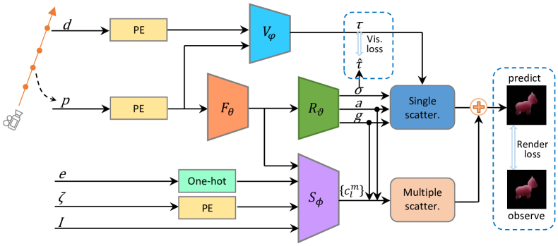
Figure 2: Our overall architecture for learning neural participating media. “PE” denotes the positional encoding and “one-hot” denotes the one-hot encoding. The rendering loss and the visibility loss correspond to the summands in Eq. 9.

Network architectures.

Figure 2 presents our overall architecture. Our neural networks are based on the coordinate-based MLP strategy, and we use frequency-based positional encoding [5, 51] $E$ to map an input coordinate $p$ to a higher dimensional vector $E(p)$ before sending it to the neural networks. Specifically, we use the MLP $R_{\vartheta}$ to predict volume density $\sigma$ (1D), scattering albedo $a$ (3D), and asymmetry parameter $g$ (1D). Meanwhile, we employ the MLP $S_{\phi}$ to learn spherical harmonic coefficients $c_{l}^{m}$. Here, $S_{\phi}$ is conditioned on the point light location $\zeta$, the point light intensity $I$, and a binary indicator $e$ which is one-hot encoded to indicate the existence of environment lighting. Since both the property network $R_{\vartheta}$ and the SH network $S_{\phi}$ takes as input the encoded coordinate, we introduce a feature network $F_{\theta}$ to predict shared features for downstream MLPs. To get the visibility for shadow rays, we train another MLP $V_{\varphi}$, which takes in the encoded direction $d$ in addition to the encoded coordinate $p$, to learn visibility values for the estimation of single scattering. In summary, we have

$$R_{\vartheta}:F_{\theta}(E(p))\rightarrow(\sigma,a,g)\quad S_{\phi}:(e,\zeta,I,F_{\theta}(E(p)))\rightarrow\{c_{l}^{m}\}\quad V_{\varphi}:(\bm{r}(t),E(d))\rightarrow\tau.$$ (7)

Note that the above $R_{\vartheta}$ learns per-location asymmetry parameter $g$ (Appendix A). Yet, for scenes with a single participating media object, we use a singe $g$ and optimize it during training.

4.2 Volume Rendering

Based on the above decomposition, we employ ray marching (Sec. 3) to numerically estimate $L_{o,s}$ and $L_{o,m}$. Hence, the final radiance $L_{o}$ of the camera ray $\bm{r}$ in Eq. 1 can be computed as:

$$L_{o}\left(\bm{r}\right)=\Sigma_{j=1}^{N}\tau\left(\bm{r}(t)\right)\left(1-\exp\left(-\sigma\left(\bm{r}(t)\right)\cdot\delta t_{j}\right)\right)\left(L_{s}+L_{m}\right),$$ (8)

where we sample $N=64$ query points in a stratified way along the ray $\bm{r}$ and $\delta t_{j}=\|\bm{r}(t_{j+1})-\bm{r}(t_{j})\|_{2}$ is the step size. For each point sample, we query the MLPs to obtain its scattering properties and SH coefficients for computing single scattering and multiple scattering.

We compute single scattering at a point based on Eq. 5. We shoot shadow rays towards light sources to get the emitted radiance $L_{e}$ according to the light types. For environment lighting, we sample $64$ directions stratified over a sphere around the point to obtain incident radiance. For a point light, we directly connect the query point to the light source. To account for the attenuation of light radiance, we query $V_{\varphi}$ to get the visibility to the light source from the query point.

For multiple scattering, we uniformly sample $K=64$ random incident directions over the sphere around each query point, evaluate the incident radiance $L_{in}$ along each direction using the learned spherical harmonic coefficients, and estimate the integral in Eq. 6 with a Monte Carlo integration $L_{m}=1/K\sum_{i=1}^{K}a\rho(\omega_{i})L_{in}(\omega_{i})$. For brevity, we omit the $\bm{r}$ notation. Note that the visibility towards the light source is not needed in the computation.

4.3 End-to-end Learning

Based on the fully differentiable pipeline, we can end-to-end learn a neural representation for each scene. The learning requires a set of posed RGB images and their lighting conditions. During each training iteration, we trace primary rays through the media. Along each primary ray, we estimate single scattering using shadow rays and compute multiple scattering contribution via the learned spherical harmonic coefficients as described in Sec. 4.2. We optimize the parameters of $F_{\theta}$, $R_{\vartheta}$, and $S_{\phi}$ by minimizing a rendering loss between the predicted radiance $L_{o}(\bm{r})$ from ray marching and the radiance $\hat{L}_{o}(\bm{r})$ from input images. To train the visibility network $V_{\varphi}$, we use the transmittance $\hat{V}_{\vartheta}$ computed from the learned volume density as the ground truth and minimize the visibility loss between the prediction $V_{\varphi}$ and the ground truth. Therefore, our loss function includes two parts:

$$\mathcal{L}=\sum_{\bm{r}\in\mathcal{R}}\|\Gamma({L}_{o}(\bm{r}))-\Gamma(\hat{L}_{o}(\bm{r}))\|_{2}^{2}+\mu\cdot\sum_{\bm{r}\in\mathcal{R},t}\|V_{\varphi}(\bm{r}(t),\bm{r}_{d})-\hat{V}_{\vartheta}(\bm{r}(t),\bm{r}_{d})\|_{2}^{2},$$ (9)

where $\Gamma(L)=L/(1+L)$ is a tone mapping function, $\mathcal{R}$ is a batch of camera rays and $\mu=0.1$ is the hyperparameter to weight the visibility loss.

4.4 Implementation Details

Our feature MLP $F_{\theta}$ has 8 fully-connected ReLU (FC-ReLU) layers with 256 channels per layer. The downstream $S_{\phi}$ consists of 8 FC-ReLU layers with 128 channels per layer, whereas the $R_{\vartheta}$ uses one such layer with 128 channels. The visibility MLP $V_{\varphi}$ has 4 FC-ReLU layers with 256 channels per layer. We set the maximum positional encoding frequency to $2^{8}$ for coordinates $p$, $2^{1}$ for directions $d$, and $2^{2}$ for the 3D location of the point light.

We train all neural networks together to minimize the loss (Eq. 9). We use the Adam [52] optimizer with its default hyperparameters and schedule the learning rate to decay from $1\times 10^{-4}$ to $1\times 10^{-5}$ over 200K iterations. For each iteration, we trace a batch of $1200$ primary rays. Note we stop the gradients from the visibility loss to the property network and the feature network so that they do not compromise the learning to match the visibility network.

5 Experiments

We firstly evaluate our method by comparing it with state-of-the-art methods on simultaneous relighting and view synthesis. Then, we demonstrate that our learned neural representations allow flexible editing and scene compositions, followed by ablation studies of this approach. Please refer to the appendices for additional results.

5.1 Experiment Settings

Compared methods.

We compare our method with state-of-the-art baselines [8, 9]. They are designed for scenes with solid objects and do not trivially extend to handle participating media, so we implement them with the new functionality to handle participating media. Please refer to the Appendix D for the implementation details.

Datasets.

We produce datasets from seven synthetic participating media scenes. The Cloud scene is heterogeneous media and the others are homogeneous media. Bunny4-VaryA and Buddha3 are set with spatially varying albedo. Bunny4-VaryG and Buddha3 are configured with spatially varying asymmetry parameters. Each scene is individually illuminated with two lighting conditions. The first one “point” has a white point light with varying intensities sampled within $50\sim 900$ and its location is randomly sampled on spheres with the radius ranging from $3.0$ to $5.0$; The second one “env + point” contains a fixed environment lighting and a randomly sampled white point light. Each dataset contains $180$ images, from which we use $170$ images for training and the remaining for validation. In addition, we prepare a test set with $30$ images for each scene to test the trained models. Each test image is rendered with a new camera pose and a new white point light that is located on a sphere of the radius $4.0$. Since Bi’s method [8] requires a collocated camera and light during training, we additionally generated such datasets for it. For the “env + point” datasets, we randomize the usage of environment lighting across images and record a binary indicator for each image.

5.2 Results

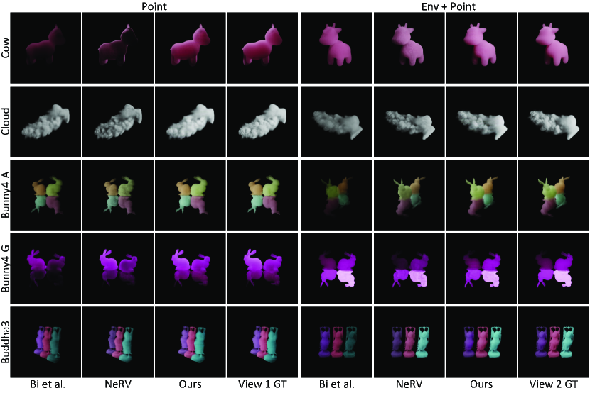
Figure 3: Qualitative comparisons of simultaneous view synthesis and relighting. The training illumination for the left half is “point” which contains a single point light. The training illumination for the right half is “env + point”. GT denotes the ground truth image.

Table 1: Quantitative comparisons on the test data for training on the “point” illumination. We measure image qualities with PSNR ($\uparrow$), SSIM ($\uparrow$) and ELPIPS ($\downarrow$) [53]. ELPIPS values below have a scale of $\times 10^{-2}$. Note the tabulated values are the mean values over all images of a test set.

Point	Cow			Cloud			Bunny4-VaryA			Bunny4-VaryG			Buddha3
Method	PSNR	SSIM	ELPIPS	PSNR	SSIM	ELPIPS	PSNR	SSIM	ELPIPS	PSNR	SSIM	ELPIPS	PSNR	SSIM	ELPIPS
Bi et al.	24.70	0.958	0.465	20.92	0.921	0.783	27.29	0.960	0.378	29.40	0.971	0.334	29.47	0.970	0.299
NeRV	25.20	0.960	0.540	25.68	0.949	0.526	27.67	0.969	0.306	26.76	0.968	0.419	28.69	0.969	0.315
Ours	34.20	0.983	0.184	33.51	0.974	0.302	34.75	0.980	0.189	33.86	0.981	0.257	33.77	0.975	0.245

Table 2: Quantitative comparisons on the test data for training on the “env + point” datasets.

Env+Point	Cow			Cloud			Bunny4-VaryA			Bunny4-VaryG			Buddha3
Method	PSNR	SSIM	ELPIPS	PSNR	SSIM	ELPIPS	PSNR	SSIM	ELPIPS	PSNR	SSIM	ELPIPS	PSNR	SSIM	ELPIPS
Bi et al.	24.84	0.960	0.501	22.18	0.934	0.709	26.65	0.958	0.464	30.03	0.974	0.285	23.41	0.938	0.679
NeRV	27.83	0.974	0.413	26.07	0.950	0.476	28.18	0.968	0.301	27.97	0.975	0.339	28.99	0.969	0.299
Ours	33.32	0.982	0.209	32.64	0.969	0.353	34.47	0.979	0.191	34.09	0.982	0.243	34.03	0.975	0.261

Relighting comparisons.

We show the qualitative comparisons of simultaneous relighting and view synthesis on the test data in Fig. 3. The left half is trained with the “point” lighting condition, whereas the right half is trained with the “env + point”. Bi’s method shows artifacts in each case as it has no mechanisms to simulate the multiple scattering that significantly affects the appearance of participating media. NeRV handles the environment illumination properly but shows artifacts on the participating media objects. Our method achieves realistic results on all test sets with either homogeneous media or heterogeneous media. Table 1 and Table 2 present the corresponding quantitative measurements, where our method overtakes the compared methods on each test set.

Using the same batch size, our training with 200K iterations on a Nvidia Quadro RTX 8000 GPU takes one day, whereas Bi’s method and NeRV takes 22h and 46h. For a $400\times 400$ image, our average inference time is $7.9$s, while Bi’s method and NeRV takes $53.2$s and $21.9$s, respectively.

Learned lighting decomposition.

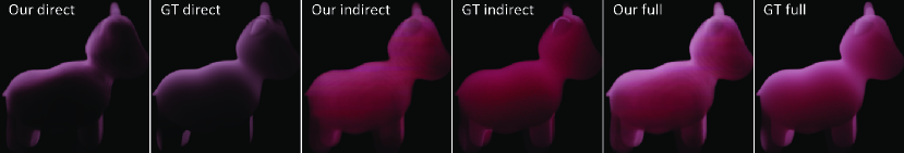
Figure 4: Lighting decompositions.

Without using any ground-truth lighting decomposition data, our method is able to learn the decomposition of lighting in an unsupervised way. Figure 4 presents our decomposed results on a test view of the Cow scene, with the single-scattering component (direct lighting) and the multiple-scattering component (indirect lighting), and the corresponding ground-truth images.

Scene editing and scene composition.

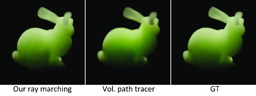
Figure 5: Ray marching vs. volume path tracing.

Our method learns neural representations for the participating media scenes. After training, we can query the neural networks to obtain the volume density, the albedo, and the phase function parameter. This allows flexible editing to achieve desired effects or insertion into a new virtual environment for content creation. In addition, we can leverage a standard rendering engine to render these data. Figure 5 compares the rendering of the learned Bunny with ray marching using the neural network and with a volumetric path tracer. To render with the path tracer, we first queried the neural network to obtain 128 x 128 x 128 data volumes of volume density and albedo. Both rendered results are visually similar to the ground truth. Figure 6 demonstrates an editing of the red channel of the albedo to achieve the red cloud and another editing of the volume density to make the cloud thinner.

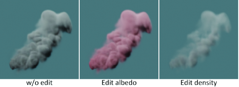
Figure 6: Edit the learned cloud.

We show in Fig. 7 that we can compose a scene consisting of our learned cow and a gold sculpture described by traditional meshes and materials (Fig. 7 bottom). Similarly, we can construct a scene composed entirely of our learned objects (Fig. 7 top). To render the composed scenes, we slice out discrete volumes with a resolution $128\times 128\times 128$ from the volume density field and the albedo field and conduct the Monte Carlo rendering in Mitsuba [54].

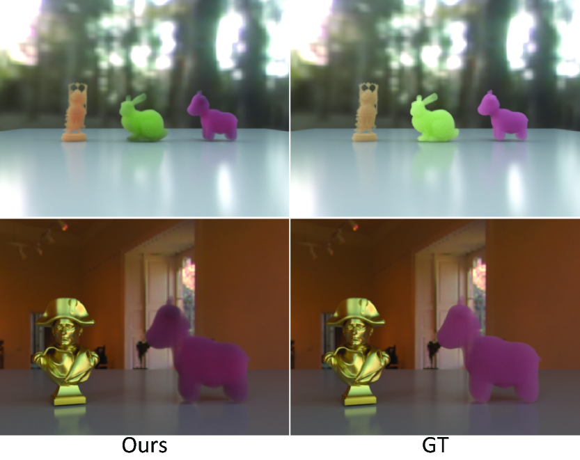
Figure 7: Scene compositions.

Scene of solid objects.

Beyond the scenes with participating media, our method can be used for scenes with solid objects. Figure 8 shows a comparison between our method and the baselines on the Dragon scene which contains glossy opaque surfaces. “Ours+BRDF” is a variant of our method that uses SH for indirect illumination, but adopts a classical BRDF model [55] and trains the neural network to predict parameters of the BRDF model as in [8, 9]. Bi’s method produces an overexposed appearance and the shadow on the floor gets faint. Our method achieves a smooth appearance and higher numerical metrics, whereas “Ours + BRDF” recovers the highlights on the glossy dragon better.

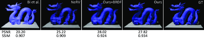
Figure 8: Comparisons on a test view of the solid Dragon with glossy surfaces. PSNR and SSIM metrics for this view are listed below images. The training illumination is from a single point light and the test illumination is a new white point light.

5.3 Ablation Studies

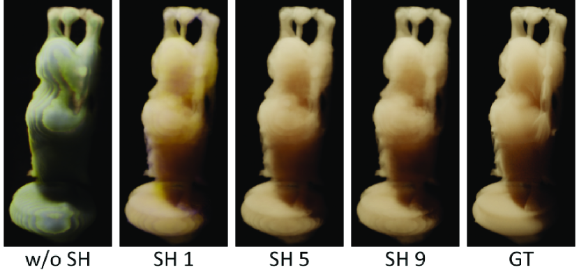
	PSNR$\uparrow$	SSIM$\uparrow$	ELPIPS$\downarrow$	Time (s)
w/o SH	25.91	0.9301	0.683	3.91
SH-1	32.53	0.9728	0.175	5.16
SH-3	32.70	0.9739	0.159	5.75
SH-5	32.87	0.9743	0.154	7.91
SH-7	32.80	0.9740	0.152	13.00
SH-9	32.61	0.9739	0.157	16.58

Figure 9: Image quality and mean inference timings of different number of spherical harmonic bands. ELPIPS metrics have a scale of $10^{-2}$. The full images, including the SH-3 and SH-7, are documented in Appendix E.

Spherical harmonic bands.

We analyze the effect of the maximum spherical harmonics band $l_{max}$ of Eq. 6 based on the Buddha scene. Figure 9 compares the same test view of each case on the left and tabulates the average quality measurements over the test set on the right. Removing the spherical harmonics from our method leads to quality drop and color shift is observed in its result. Based on the numerical metrics and inference timings, we select the $l_{max}=5$ for other experiments.

Scattering function.

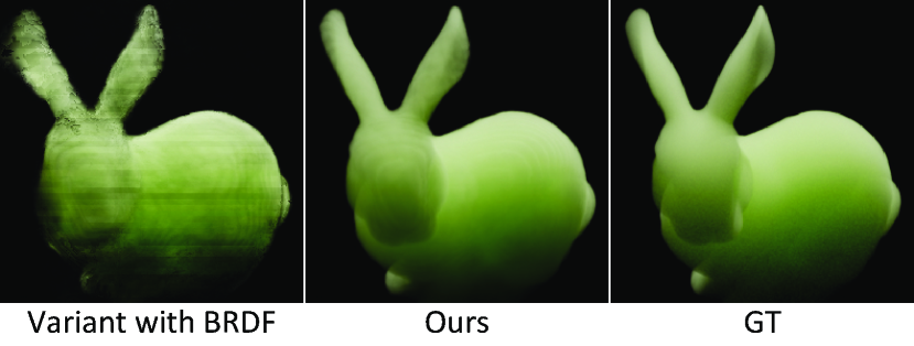
Figure 10: Compare Ours+BRDF and Ours with phase function.

We show in Fig. 8 that our method with the HG phase function can be applied to a scene of solid objects. In addition, we conduct an ablation by applying the variant “Ours+BRDF” to the Bunny scene of participating media. Figure 10 shows that the variant has difficulty in learning the volume density and leads to many cracks, while the proposed method performs robustly on this scene.

6 Limitations and Future Work

Real-world scenes.

In this work, we learn neural representations from synthetic datasets with varying but known lighting conditions. Also, the camera poses are available to the method. It would be interesting to extend this method to handle participating media captured from real-world scenes with unknown lighting conditions and unknown camera poses. In that case, the illumination and camera poses of the scenes need to be estimated in the first place.

Glossy reflections.

For scenes with glossy solid objects (Fig. 8), our method tends to reproduce a smooth appearance and the glossy highlights are not as sharp as the ground truth. An avenue for future research would be to develop methods to recover the glossy reflections better.

Generalizability.

Our ray marching with the trained neural network generalizes well to unseen light intensities and light locations that are in the range of the training data. That said, its generalization is in an interpolation manner. For light intensities and light locations that are outside of the training range, the generalization quality of the neural network gradually decreases. Please refer to the Appendix H for the analysis on the generalization quality.

Media within refractive boundaries.

Our method achieves realistic results for participating media without refractive boundaries, like cloud, fog, and wax figure. Applying our method to participating media within refractive boundaries, like wine in a glass, entails further work as the refractive boundaries cause ambiguities due to deflecting the camera rays and the light rays.

7 Conclusion

We have proposed a novel method for participating media reconstruction from observed images with varying but known illumination. We propose to simulate direct illumination with Monte Carlo ray tracing and approximate indirect illumination with learned spherical harmonics. This enables our approach to learn to decompose the illumination as direct and indirect components in an unsupervised manner. Our method learns a disentangled neural representation with volume density, scattering albedo and phase function parameters for participating media, and we demonstrated its flexible applications in relighting, scene editing and scene compositions.

Appendices

Appendix A Phase Function Details

Our phase function for participating media (Sec. 4.1) is the Henyey-Greenstein (HG) function [50]

$$p(\omega_{o},\omega_{i},g)=\frac{1}{4\pi}\frac{1-g^{2}}{\left(1+g^{2}+2g\cos{\theta}\right)^{3/2}},$$ (10)

where $\theta$ is the angle between the outgoing direction $\omega_{o}$ and the incident direction $\omega_{i}$. For the notations of directions, we use the convention that both the incident and outgoing rays point away from a scattering location. $g$ is called the asymmetry parameter that is in $(-1,1)$. A positive $g$ value is for forward scattering, a negative $g$ value is for backward scattering, and the zero value is for isotropic scattering.

Same as in [8, 9], our BRDF function for the experiment on solid objects (Sec. 5.2) is the analytical model [55] which combines a specular component using the ggx distribution [56] and a diffuse component.

Appendix B Spherical Harmonics Details

In Sec. 4.1 of the main paper, we propose to represent the incident radiance due to multiple scattering with spherical harmonics. Spherical Harmonics (SH) are orthonormal basis defined on complex numbers over the unit sphere. Since our radiance function is defined in the real number domain, our SH basis functions $Y_{l}^{m}(\omega_{i})\left(0\leq l\leq l_{max},-l\leq m\leq l\right)$ in Eq. 6 are real spherical harmonic functions

$$Y_{l}^{m}(\theta_{i},\phi_{i})=\begin{cases}\sqrt{2}K_{l}^{m}\cos(m\phi_{i})P_{l}^{m}(\cos\theta_{i})&\text{$m>0$}\\ K_{l}^{m}P_{l}^{m}(\cos\theta_{i})&\text{$m=0$}\\ \sqrt{2}K_{l}^{m}\sin(-m\phi_{i})P_{l}^{-m}(\cos\theta_{i})&\text{$m<0$,}\end{cases}$$ (11)

where $(\theta_{i},\phi_{i})$ are the spherical coordinates of the direction $\omega_{i}$ that is in the Cartesian coordinate system, $K_{l}^{m}=\sqrt{\frac{(1+2l)}{4\pi}\frac{(l-\left|m\right|)!}{(l+\left|m\right|)!}}$ is a normalization factor, and $P_{l}^{m}$ are the associated Legendre polynomials. Then, the incident radiance function $\widetilde{L}(\omega_{i})$ can be computed using the SH basis

$$\widetilde{L}(\omega_{i})=\mathcal{F}\left(\sum_{l=0}^{l_{max}}\sum_{m=-l}^{l}c_{l}^{m}Y_{l}^{m}(\omega_{i})\right),$$ (12)

where $c_{l}^{m}\in\mathbb{R}^{3}$ are SH coefficients, $l_{max}$ is the maximum SH band, and $\mathcal{F}(x)=\max(0,x)$ ensures non-negative incident radiance.

In each training iteration, we sample $K=64$ random incident directions $\{\omega_{i}\}_{i=1}^{K}$ and evaluate the $Y_{l}^{m}(\omega_{i})$. To reduce the computational cost, we reuse these incident directions and the evaluated $Y_{l}^{m}(\omega_{i})$ for all point samples along the primary rays of this batch.

Appendix C Additional Implementation Details of Our Method

Training details.

We end-to-end train our model to learn a separate neural representation of each scene. In each training iteration, we randomly draw a batch of $1200$ primary rays across all training views. Our visibility network is trained to match the learned scene geometry by the property network, so it is optimized according to the visibility values computed from the volume density, without requiring ground-truth visibility. We cut off the gradient from the render loss to the visibility network. Meanwhile, we cut off the gradient from the visibility loss to the property network so that it does not degrade its learning of the volume density.

Inference details.

Our inference uses the same setting as the training. We draw $64$ point samples along each camera ray to query our model. The number of incident directions for computing indirect illumination is $64$. We set the number of shadow rays to $1$ for the point light, whereas we use $32$ shadow rays for the environment lighting.

Appendix D Implementation details of the two baselines

For our comparisons, we implemented the Neural Reflectance Field [8] and NeRV [9] as our baselines. Since they were designed for scenes with solid objects, we adapt them to cope with participating media.

Our implementation of the Neural Reflectance Field [8] baseline uses the same neural network architecture and positional encoding as in the original paper. Specifically, we implement the dual-network design with a coarse network and a fine network. Each neural network is an MLP consisting of $14$ fully-connected ReLU layers with $256$ neurons per layer. Also, we apply frequency-based positional encoding to transform the input 3D coordinates with a maximum frequency $2^{10}$. Different from the eight-channel output in the original paper, we have a four-channel output consisting of a 1-D volume density and a 3-D scattering albedo. Along each ray, we draw $64$ stratifed point samples for the coarse network and $128$ point samples for the fine network.

In our implementation of the NeRV [9] baseline, we utilize an MLP with $8$ fully-connected ReLU layers to compute the physical properties. Each layer has $256$ neurons. In addition, we employ a visibility MLP [9] to compute a 1-D visibility and a 1-D expected termination depth. The visibiliy MLP firstly processes the encoded coordinates using $8$ fully-connected ReLU layers with $256$ neurons per layer to get an 8-D output. The output, concatenated with the encoded directions, is further processed by $4$ fully-connected ReLU layers with $128$ neurons per layer. The maximum positional encoding frequencies for 3D coordinates and directions are $2^{7}$ and $2^{4}$, respectively. Along each camera ray, we take $64$ stratified samples, same as in our method. We trace one shadow ray for the point light source and $32$ shadow rays for the environment lighting. For the “point” illumination, we uniformly take $128$ random directions for the first indirect bounces at the termination depth along a ray. For the “env + point” illumination, we set the number of first indirect bounces to $32$.

Appendix E Additional images for the spherical harmonic band ablation

In the ablation study of the maximum spherical harmonic band (Sec. 5.3), we show the results of SH-$1$, SH-$5$, and SH-$9$. We present the full comparison with SH-3 and SH-5 in Fig. 11. The quantitative metrics are listed in the right table of Fig. 9 (Sec. 5.3). Note that SH-5 achieves the qualitative result that is similar to SH-7 and SH-9, but SH-5 gives higher numerical performance than others (Fig. 11).

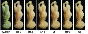
Figure 11: Qualitative comparisons of different settings of the maximum spherical harmonic band from SH-$1$ to SH-$9$. “w/o SH” denotes without using spherical harmonics and “GT” denotes the ground truth.

Appendix F Additional quantitative results for participating media scenes

F.1 Scenes trained on the “point”

Table 3 presents additional numerical results for the single Bunny and Buddha scenes when using the “point” training illumination. Each test view has a new point light. The tabulated values are the mean values over images of the test set. Our approach outperforms the two baselines quantitatively.

Table 3: Quantitative comparisons on the test data. Image qualities are measured with PSNR ($\uparrow$), SSIM ($\uparrow$) and ELPIPS ($\downarrow$) [53]. ELPIPS values have a scale of $\times 10^{-2}$.

Point	Bunny			Buddha
Method	PSNR	SSIM	ELPIPS	PSNR	SSIM	ELPIPS
Bi et al.	22.46	0.933	0.720	23.62	0.951	0.518
NeRV	24.57	0.951	0.627	25.47	0.959	0.432
Ours	33.49	0.982	0.209	32.87	0.974	0.154

F.2 Scenes trained on the “env + point”

Accordingly, Table 4 presents quantitative results for the Bunny and the Buddha scenes when they are trained with the “env + point” illumination. Each test view has a single novel point light. Our method numerically performs better than the baselines.

Table 4: Quantitative comparisons on the Bunny and the Buddha scene when they are trained with the “env + point” illumination. The PSNR ($\uparrow$), SSIM ($\uparrow$) and ELPIPS ($\downarrow$) [53] values are averaged over all images of a test set. ELPIPS values have a scale of $\times 10^{-2}$.

Env+Point	Bunny			Buddha
Method	PSNR	SSIM	ELPIPS	PSNR	SSIM	ELPIPS
Bi et al.	22.82	0.935	0.709	24.20	0.956	0.466
NeRV	25.24	0.959	0.597	27.36	0.968	0.345
Ours	32.93	0.980	0.293	32.74	0.976	0.204

Appendix G Quantitative results for scenes of solid objects

In Table 5, we show the quantitative results on the Dragon scene and the Armadillo scene that contain glossy solid objects. Bi’s method and the NeRV method use the parameter settings as described in Appendix D. Our method retains the same parameter settings as those for the participating media scenes. “Ours + BRDF” is a variant of our method that uses a BRDF function as the scattering function. We experimentally set its maximum spherical harmonic band to $1$ and set the highest positional encoding frequency to $2^{7}$. Our method achieves higher quantitative metrics compared to the baselines and the variant.

Figure 8 of the main paper shows a comparison on one test view of the Dragon scene. Bi’s method recovers the highlights on surfaces, but it produces an overexposed appearance and leads to faint shadows. Our method produces a smooth appearance and properly cast the shadow according to the novel lighting.

Table 5: Quantitative comparisons on two scenes with glossy solid objects. The scenes are trained with the “point” illumination and tested under novel lighting. The PSNR ($\uparrow$), SSIM ($\uparrow$) and ELPIPS ($\downarrow$) [53] are the averaged value over a test set. ELPIPS values have a scale of $\times 10^{-2}$.

	Dragon			Armadillo
Method	PSNR	SSIM	ELPIPS	PSNR	SSIM	ELPIPS
Bi et al.	19.60	0.897	1.358	19.19	0.897	1.243
NeRV	26.60	0.917	0.902	25.32	0.893	1.034
Ours + BRDF	28.32	0.931	0.692	26.46	0.917	0.847
Ours	28.50	0.942	0.564	26.60	0.924	0.753

Appendix H Generalization quality

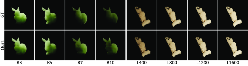
Figure 12: Qualitative comparisons of generalization on light location and light intensity.

Bunny	Light distance (m)
	3	5	7	10
PSNR	31.39	29.87	23.14	16.96
SSIM	0.970	0.965	0.922	0.865
ELPIPS	0.359	0.388	0.923	1.740

Buddha	Light intensity
	400	800	1200	1600
PSNR	32.82	33.04	31.91	28.47
SSIM	0.982	0.984	0.981	0.974
ELPIPS	0.204	0.195	0.219	0.235

Figure 13: Quantitative results for investigating the generalization on the light locations and light intensities. ELPIPS metrics have a scale of $10^{-2}$.

Generalization quality for light distance.

We used the Bunny scene in this experiment. During training, the point light’s distance to the center of the bunny is stratified sampled from the range $(3,5)$. We then build four test sets, each with 20 views; we set the point light’s distance for the test sets as $3$, $5$, $7$, and $10$, individually. The light intensity is set to 600. We run the trained neural network on each test set. The image results are presented on the left of Fig. 12 and the numerical performance is shown in the left table of Fig. 13. The trained neural network performs relatively well when the test point light’s distance is close to those in training, and the numerical performance gradually drops when the test point light moves away from the training manifold.

Generalization quality for light intensity.

We used the Buddha scene in this experiment. The training intensity values were stratified sampled from $50$ to $900$. We generate four test sets with the same 20 camera views. The point light is put at a distance $4$ for all test sets. Also, we set the test light intensity as $400$, $800$, $1200$, and $1600$, respectively. Same as before, we run the trained neural network on each test set. The graphical comparisons and numerical metrics are shown on the right of Fig. 12 and Fig. 13. We observed that the trained neural network achieves high numerical performance when the test light intensity is within the range of the training intensity. For testing intensity outside of the training range, the numerical performance decreases.

References

- Gu et al. [2008] Jinwei Gu, Shree Nayar, Eitan Grinspun, Peter Belhumeur, and Ravi Ramamoorthi. Compressive structured light for recovering inhomogeneous participating media. In European Conference on Computer Vision, pages 845–858. Springer, 2008.
- Hawkins et al. [2005] Tim Hawkins, Per Einarsson, and Paul Debevec. Acquisition of time-varying participating media. ACM Transactions on Graphics (ToG), 24(3):812–815, 2005.
- Fuchs et al. [2007] Christian Fuchs, Tongbo Chen, Michael Goesele, Holger Theisel, and Hans-Peter Seidel. Density estimation for dynamic volumes. Computers & Graphics, 31(2):205–211, 2007.
- Hasinoff and Kutulakos [2007] Samuel W Hasinoff and Kiriakos N Kutulakos. Photo-consistent reconstruction of semitransparent scenes by density-sheet decomposition. IEEE Transactions on Pattern Analysis and Machine Intelligence, 29(5):870–885, 2007.
- Mildenhall et al. [2020] Ben Mildenhall, Pratul P Srinivasan, Matthew Tancik, Jonathan T Barron, Ravi Ramamoorthi, and Ren Ng. NeRF: Representing scenes as neural radiance fields for view synthesis. In European Conference on Computer Vision, pages 405–421. Springer, 2020.
- Lombardi et al. [2019] Stephen Lombardi, Tomas Simon, Jason Saragih, Gabriel Schwartz, Andreas Lehrmann, and Yaser Sheikh. Neural volumes: learning dynamic renderable volumes from images. ACM Transactions on Graphics (TOG), 38(4):1–14, 2019.
- Sitzmann et al. [2019a] Vincent Sitzmann, Michael Zollhöfer, and Gordon Wetzstein. Scene representation networks: Continuous 3D-structure-aware neural scene representations. In Advances in Neural Information Processing Systems, pages 1121–1132, 2019a.
- Bi et al. [2020a] Sai Bi, Zexiang Xu, Pratul Srinivasan, Ben Mildenhall, Kalyan Sunkavalli, Miloš Hašan, Yannick Hold-Geoffroy, David Kriegman, and Ravi Ramamoorthi. Neural reflectance fields for appearance acquisition. arXiv preprint arXiv:2008.03824, 2020a.
- Srinivasan et al. [2021] Pratul P Srinivasan, Boyang Deng, Xiuming Zhang, Matthew Tancik, Ben Mildenhall, and Jonathan T Barron. NeRV: Neural reflectance and visibility fields for relighting and view synthesis. In Proceedings of the IEEE/CVF Conference on Computer Vision and Pattern Recognition, pages 7495–7504, 2021.
- Mukaigawa et al. [2010] Yasuhiro Mukaigawa, Yasushi Yagi, and Ramesh Raskar. Analysis of light transport in scattering media. In 2010 IEEE Computer Society Conference on Computer Vision and Pattern Recognition, pages 153–160. IEEE, 2010.
- Eslami et al. [2018] SM Ali Eslami, Danilo Jimenez Rezende, Frederic Besse, Fabio Viola, Ari S Morcos, Marta Garnelo, Avraham Ruderman, Andrei A Rusu, Ivo Danihelka, Karol Gregor, et al. Neural scene representation and rendering. Science, 360(6394):1204–1210, 2018.
- Satilmis et al. [2016] Pinar Satilmis, Thomas Bashford-Rogers, Alan Chalmers, and Kurt Debattista. A machine-learning-driven sky model. IEEE Computer Graphics and Applications, 37(1):80–91, 2016.
- Zheng and Zheng [2017a] Quan Zheng and Changwen Zheng. NeuroLens: Data-driven camera lens simulation using neural networks. Computer Graphics Forum, 36(8):390–401, 2017a.
- Zheng and Zheng [2017b] Quan Zheng and Changwen Zheng. Adaptive sparse polynomial regression for camera lens simulation. The Visual Computer, 33(6-8):715–724, 2017b.
- Sitzmann et al. [2019b] Vincent Sitzmann, Justus Thies, Felix Heide, Matthias Nießner, Gordon Wetzstein, and Michael Zollhofer. DeepVoxels: Learning persistent 3D feature embeddings. In Proceedings of the IEEE/CVF Conference on Computer Vision and Pattern Recognition, pages 2437–2446, 2019b.
- Peng et al. [2020] Songyou Peng, Michael Niemeyer, Lars Mescheder, Marc Pollefeys, and Andreas Geiger. Convolutional occupancy networks. In Computer Vision–ECCV 2020: 16th European Conference, Glasgow, UK, August 23–28, 2020, Proceedings, Part III 16, pages 523–540. Springer, 2020.
- Flynn et al. [2019] John Flynn, Michael Broxton, Paul Debevec, Matthew DuVall, Graham Fyffe, Ryan Overbeck, Noah Snavely, and Richard Tucker. DeepView: View synthesis with learned gradient descent. In Proceedings of the IEEE/CVF Conference on Computer Vision and Pattern Recognition, pages 2367–2376, 2019.
- Zhou et al. [2018] Tinghui Zhou, Richard Tucker, John Flynn, Graham Fyffe, and Noah Snavely. Stereo magnification: learning view synthesis using multiplane images. ACM Transactions on Graphics (TOG), 37(4):1–12, 2018.
- Zhang et al. [2021] Xiuming Zhang, Sean Fanello, Yun-Ta Tsai, Tiancheng Sun, Tianfan Xue, Rohit Pandey, Sergio Orts-Escolano, Philip Davidson, Christoph Rhemann, Paul Debevec, et al. Neural light transport for relighting and view synthesis. ACM Transactions on Graphics (TOG), 40(1):1–17, 2021.
- Park et al. [2019] Jeong Joon Park, Peter Florence, Julian Straub, Richard Newcombe, and Steven Lovegrove. DeepSDF: Learning continuous signed distance functions for shape representation. In Proceedings of the IEEE/CVF Conference on Computer Vision and Pattern Recognition, pages 165–174, 2019.
- Chabra et al. [2020] Rohan Chabra, Jan E Lenssen, Eddy Ilg, Tanner Schmidt, Julian Straub, Steven Lovegrove, and Richard Newcombe. Deep local shapes: Learning local SDF priors for detailed 3D reconstruction. In European Conference on Computer Vision, pages 608–625. Springer, 2020.
- Chen and Zhang [2019] Zhiqin Chen and Hao Zhang. Learning implicit fields for generative shape modeling. In Proceedings of the IEEE/CVF Conference on Computer Vision and Pattern Recognition, pages 5939–5948, 2019.
- Mescheder et al. [2019] Lars Mescheder, Michael Oechsle, Michael Niemeyer, Sebastian Nowozin, and Andreas Geiger. Occupancy networks: Learning 3D reconstruction in function space. In Proceedings of the IEEE/CVF Conference on Computer Vision and Pattern Recognition, pages 4460–4470, 2019.
- Liu et al. [2020a] Lingjie Liu, Jiatao Gu, Kyaw Zaw Lin, Tat-Seng Chua, and Christian Theobalt. Neural sparse voxel fields. Advances in Neural Information Processing Systems, 33, 2020a.
- Saito et al. [2019] Shunsuke Saito, Zeng Huang, Ryota Natsume, Shigeo Morishima, Angjoo Kanazawa, and Hao Li. PIFu: Pixel-aligned implicit function for high-resolution clothed human digitization. In Proceedings of the IEEE/CVF International Conference on Computer Vision, pages 2304–2314, 2019.
- Xu et al. [2019] Qiangeng Xu, Weiyue Wang, Duygu Ceylan, Radomir Mech, and Ulrich Neumann. DISN: Deep implicit surface network for high-quality single-view 3D reconstruction. Advances in Neural Information Processing Systems, 32:492–502, 2019.
- Sitzmann et al. [2020] Vincent Sitzmann, Julien Martel, Alexander Bergman, David Lindell, and Gordon Wetzstein. Implicit neural representations with periodic activation functions. Advances in Neural Information Processing Systems, 33, 2020.
- Zheng et al. [2020] Quan Zheng, Vahid Babaei, Gordon Wetzstein, Hans-Peter Seidel, Matthias Zwicker, and Gurprit Singh. Neural light field 3D printing. ACM Transactions on Graphics (TOG), 39(6):1–12, 2020.
- Liu et al. [2020b] Shaohui Liu, Yinda Zhang, Songyou Peng, Boxin Shi, Marc Pollefeys, and Zhaopeng Cui. DIST: Rendering deep implicit signed distance function with differentiable sphere tracing. In Proceedings of the IEEE/CVF Conference on Computer Vision and Pattern Recognition, pages 2019–2028, 2020b.
- Srinivasan et al. [2017] Pratul P Srinivasan, Tongzhou Wang, Ashwin Sreelal, Ravi Ramamoorthi, and Ren Ng. Learning to synthesize a 4D RGBD light field from a single image. In Proceedings of the IEEE International Conference on Computer Vision, pages 2243–2251, 2017.
- Srinivasan et al. [2019] Pratul P Srinivasan, Richard Tucker, Jonathan T Barron, Ravi Ramamoorthi, Ren Ng, and Noah Snavely. Pushing the boundaries of view extrapolation with multiplane images. In Proceedings of the IEEE/CVF Conference on Computer Vision and Pattern Recognition, pages 175–184, 2019.
- Goesele et al. [2004] Michael Goesele, Hendrik P. A. Lensch, Jochen Lang, Christian Fuchs, and Hans-Peter Seidel. DISCO: Acquisition of translucent objects. In ACM SIGGRAPH 2004 Papers, pages 835–844, New York, NY, USA, 2004. Association for Computing Machinery.
- Gkioulekas et al. [2016] Ioannis Gkioulekas, Anat Levin, and Todd Zickler. An evaluation of computational imaging techniques for heterogeneous inverse scattering. In European Conference on Computer Vision, pages 685–701. Springer, 2016.
- Gkioulekas et al. [2013] Ioannis Gkioulekas, Shuang Zhao, Kavita Bala, Todd Zickler, and Anat Levin. Inverse volume rendering with material dictionaries. ACM Transactions on Graphics (TOG), 32(6):1–13, 2013.
- Azinovic et al. [2019] Dejan Azinovic, Tzu-Mao Li, Anton Kaplanyan, and Matthias Nießner. Inverse path tracing for joint material and lighting estimation. In Proceedings of the IEEE/CVF Conference on Computer Vision and Pattern Recognition, pages 2447–2456, 2019.
- Che et al. [2020] Chengqian Che, Fujun Luan, Shuang Zhao, Kavita Bala, and Ioannis Gkioulekas. Towards learning-based inverse subsurface scattering. In 2020 IEEE International Conference on Computational Photography (ICCP), pages 1–12. IEEE, 2020.
- Zhang et al. [2019] Cheng Zhang, Lifan Wu, Changxi Zheng, Ioannis Gkioulekas, Ravi Ramamoorthi, and Shuang Zhao. A differential theory of radiative transfer. ACM Transactions on Graphics (TOG), 38(6):1–16, 2019.
- Dellaert and Yen-Chen [2020] Frank Dellaert and Lin Yen-Chen. Neural volume rendering: NeRF and beyond. arXiv preprint arXiv:2101.05204, 2020.
- Martin-Brualla et al. [2021] Ricardo Martin-Brualla, Noha Radwan, Mehdi SM Sajjadi, Jonathan T Barron, Alexey Dosovitskiy, and Daniel Duckworth. NeRF in the wild: Neural radiance fields for unconstrained photo collections. In Proceedings of the IEEE/CVF Conference on Computer Vision and Pattern Recognition, pages 7210–7219, 2021.
- Schwarz et al. [2020] Katja Schwarz, Yiyi Liao, Michael Niemeyer, and Andreas Geiger. GRAF: Generative radiance fields for 3D-aware image synthesis. Advances in Neural Information Processing Systems, 33, 2020.
- Boss et al. [2021] Mark Boss, Raphael Braun, Varun Jampani, Jonathan T Barron, Ce Liu, and Hendrik Lensch. NeRD: Neural reflectance decomposition from image collections. In Proceedings of the IEEE/CVF International Conference on Computer Vision, pages 12684–12694, 2021.
- Jarosz et al. [2011] Wojciech Jarosz, Derek Nowrouzezahrai, Iman Sadeghi, and Henrik Wann Jensen. A comprehensive theory of volumetric radiance estimation using photon points and beams. ACM Transactions on Graphics (TOG), 30(1):1–19, 2011.
- Zheng and Zheng [2015] Quan Zheng and Chang-Wen Zheng. Visual importance-based adaptive photon tracing. The Visual Computer, 31(6):1001–1010, 2015.
- Novák et al. [2018] Jan Novák, Iliyan Georgiev, Johannes Hanika, and Wojciech Jarosz. Monte Carlo methods for volumetric light transport simulation. Computer Graphics Forum, 37(2):551–576, 2018.
- Bi et al. [2020b] Sai Bi, Zexiang Xu, Kalyan Sunkavalli, Miloš Hašan, Yannick Hold-Geoffroy, David Kriegman, and Ravi Ramamoorthi. Deep reflectance volumes: Relightable reconstructions from multi-view photometric images. In Computer Vision–ECCV 2020: 16th European Conference, Glasgow, UK, August 23–28, 2020, Proceedings, Part III 16, pages 294–311. Springer, 2020b.
- Guo et al. [2020] Michelle Guo, Alireza Fathi, Jiajun Wu, and Thomas Funkhouser. Object-centric neural scene rendering. arXiv preprint arXiv:2012.08503, 2020.
- Yu et al. [2021] Alex Yu, Ruilong Li, Matthew Tancik, Hao Li, Ren Ng, and Angjoo Kanazawa. PlenOctrees for real-time rendering of neural radiance fields. In ICCV, 2021.
- Lafortune and Willems [1996] Eric P Lafortune and Yves D Willems. Rendering participating media with bidirectional path tracing. In Eurographics Workshop on Rendering Techniques, pages 91–100. Springer, 1996.
- Kniss et al. [2003] Joe Kniss, Simon Premoze, Charles Hansen, Peter Shirley, and Allen McPherson. A model for volume lighting and modeling. IEEE Transactions on Visualization and Computer Graphics, 9(2):150–162, 2003.
- Henyey and Greenstein [1941] Louis G Henyey and Jesse Leonard Greenstein. Diffuse radiation in the galaxy. The Astrophysical Journal, 93:70–83, 1941.
- Tancik et al. [2020] Matthew Tancik, Pratul P. Srinivasan, Ben Mildenhall, Sara Fridovich-Keil, Nithin Raghavan, Utkarsh Singhal, Ravi Ramamoorthi, Jonathan T. Barron, and Ren Ng. Fourier features let networks learn high frequency functions in low dimensional domains. NeurIPS, 2020.
- Kingma and Ba [2015] Diederik P. Kingma and Jimmy Ba. Adam: A method for stochastic optimization. In Yoshua Bengio and Yann LeCun, editors, 3rd International Conference on Learning Representations, ICLR 2015, San Diego, CA, USA, May 7-9, 2015, Conference Track Proceedings, 2015.
- Kettunen et al. [2019] Markus Kettunen, Erik Härkönen, and Jaakko Lehtinen. E-LPIPS: robust perceptual image similarity via random transformation ensembles. arXiv preprint arXiv:1906.03973, 2019.
- Jakob [2010] Wenzel Jakob. Mitsuba renderer, 2010. http://www.mitsuba-renderer.org.
- Karis [2013] Brian Karis. Real shading in unreal engine 4. Proc. Physically Based Shading Theory Practice, 4:3, 2013.
- Walter et al. [2007] Bruce Walter, Stephen R. Marschner, Hongsong Li, and Kenneth E. Torrance. Microfacet models for refraction through rough surfaces. In Proceedings of the Eurographics Symposium on Rendering Techniques, Grenoble, France, 2007, pages 195–206. Eurographics Association, 2007.