Hidden Symmetry in 1D Localization

1. Introduction

For description of 1D disordered systems it is convenient to use the transfer matrix $T$, relating the amplitudes of plane waves on the left ($Ae^{ikx}+Be^{-ikx}$) and on the right ($Ce^{ikx}+De^{-ikx}$) of a scatterer,

$$\left(\begin{array}[]{cc}A\\ B\end{array}\right)\,=T\left(\begin{array}[]{cc}C\\ D\end{array}\right)\,.$$

In the presence time-reversal invariance, the matrix $T$ can be parametrized in the form [1]

$$T=\left(\begin{array}[]{cc}\!\!\!1/t\!&\!-r/t\!\!\\ \!\!-r^{*}/t^{*}\!&\!1/t^{*}\!\!\!\end{array}\right)\,=\left(\begin{array}[]{cc}\!\!\sqrt{\rho\!+\!1}\,e^{i\varphi}\!\!&\!\!\sqrt{\rho}\,e^{i\theta}\!\!\\ \!\!\sqrt{\rho}\,e^{-i\theta}\!\!&\!\!\sqrt{\rho\!+\!1}\,e^{-i\varphi}\!\!\end{array}\right)\,,$$

where $t$ and $r$ are the amplitudes of transmission and reflection, while $\rho=|r/t|^{2}$ is the dimensionless Landauer resistance [2]. For the successive arrangement of scatterers their transfer matrices are multiplied. For a weak scatterer its transfer matrix $T$ is close to the unit one, which allows to derive the differential evolution equations for its parameters, and in particular for the Landauer resistance $\rho$.

In the random phase approximation (when distributions of $\varphi$ and $\theta$ are considered as uniform) such equation for the distribution $P(\rho)$ has a form [3]–[8]

$$\frac{\partial P(\rho)}{\partial L}=D\,\frac{\partial}{\partial\rho}\left[\,\rho(1\!+\!\rho)\,\frac{\partial P(\rho)}{\partial\rho}\,\right]\,$$

and describes evolution of the initial distribution $P_{0}(\rho)=\delta(\rho)$ at zero length $L$ to the log-normal distribution in the large $L$ limit.

As shown in the paper [9], the distributions of phases $\varphi$ and $\theta$ change essentially, if semi-transparent boundaries are introduced between the disordered system and the ideal leads connected to it. Then the more general equation arises

$$\frac{\partial P(\rho)}{\partial L}=D\,\frac{\partial}{\partial\rho}\left[\,-\gamma(1\!+\!2\rho)P(\rho)+\rho(1\!+\!\rho)\,\frac{\partial P(\rho)}{\partial\rho}\,\right]\,,$$

which reduces to (2) in the random phase approximation. The latter approximation is working sufficiently good in the deep of the allowed band for the ”natural” ideal leads (made from the same material as a disordered system, but without impurities), as it is usually accepted in the theoretical papers (see references in [10, 11, 12]); a situation in the forbidden band is considered infrequently [13, 14, 15] and only on the level of the wave functions. To study the evolution of $P(\rho)$ for the arbitrary Fermi level position (including the forbidden band), one should explicitly introduce the foreign ideal leads made from the good metal; as a result, the still more general equation arises [16],

$$\frac{\partial P(\rho)}{\partial L}=D\,\frac{\partial}{\partial\rho}\left[\,-\gamma_{1}(1\!+\!2\rho)P(\rho)-\vphantom{\frac{1}{2}}\right.$$

$$\left.\,-2\gamma_{2}\sqrt{\rho(1\!+\!\rho)}P(\rho)+\rho(1\!+\!\rho)\,\frac{\partial P(\rho)}{\partial\rho}\,\right]\,,$$

whose coefficients are determined by the stationary phase distribution (see Eqs. 29, 31 below) in the large $L$ limit. Equation (4) reduces to (3) with $\gamma=\gamma_{1}+\gamma_{2}$ in the region of large $L$, when typical values of $\rho$ are large. Meanwhile, it becomes clear that the random phase approximation is violated due to internal reasons and a change of the boundary conditions is not essential for it. According to the paper [16], the distribution $P(\rho)$ in the limit of large $L$ has the log-normal form

$$P(\rho)=\frac{1}{\rho\sqrt{4\pi DL}}\exp\left\{-\frac{[\ln\rho-vL]^{2}}{4DL}\right\}\,$$

with $v=(2\gamma\!+\!1)D$, whose parameters are determined by the internal properties of the system, and does not depend on the boundary conditions. Fig.1 illustrates the dependence of the parameter $\gamma$ on the quantity ${\cal E}/W^{4/3}$, where ${\cal E}$ is the Fermi energy counted from the lower edge of the initial band, and $W$ is the amplitude of a random potetial; all energies are measured in the units of the hopping integral for the 1D Anderson model (see below Eq.9). One can see that the parameter $\gamma$ is formally always finite but takes small values in the deep of the allowed band, in correspondence with the random phase approximation.

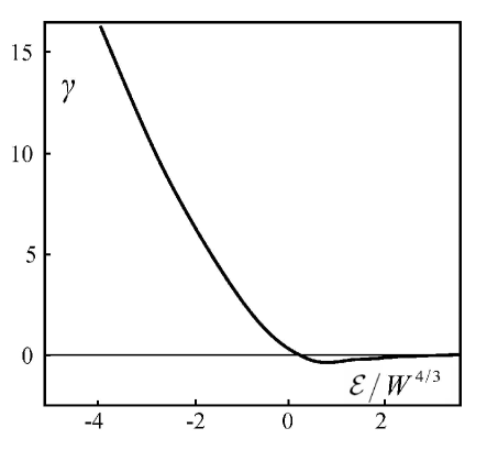
Figure 1: Parameter $\gamma$ in equation (2), corresponding to the limit of large $l$, as function of the energy ${\cal E}$, counted from the lower edge of the initial band.

One can see that two statements were made in the papers [9, 16], which look hardly compatible. On one hand, variation of the boundary conditions essentially affects the distribution of phases, which generally changes the parameters of the evolution equations (2–4) and even its structure. On the other hand, these changes have no influence on the form of the limiting distribution (5) in the large $L$ region. Validity of these two statements means that the system obeys a hidden symmetry, i.e. invariance of the physical quantities respective to a certain class of transformations. From the theoretical viewpoint, revelation of the hidden symmetry is of the evident interest, indicating the possibility of essential simplifications. From the practical point, one cannot differ the real physical effects from the fictive ones, if the nature of hidden invariance is not clarified. Revelation of this invariance appears to be very nontrivial and we demonstrate it below for a set of transformations discussed in Ref. [16] and related with a change of properties of the ideal leads attached to the system.

Let explain the origin of two indicated statements. Under a change of the boundary conditions, the transfer matrix $T$ transforms to $\tilde{T}=T_{l}TT_{r}$, where $T_{l}$ and $T_{r}$ are the edge matrices, related amplitudes of waves on the left and on the right of the corresponding interface. Thereby, the change of the boundary conditions leads to the linear transformation of the trasfer matrix elements. The linear transformation does not affect the growth exponents for the second and forth moments of the matrix elements, which can be found for a given matrix $T$ and hence are determined by internal properties of the system. Knowledge of these two exponents allows to establish ”the diffusion constant” $D$ and ”the drift velocity” $v$ in the limiting distribution (5), which consequently does not depend on the boundary conditions [16]; in particular, the behavior of the parameter $\gamma$ (Fig.1) was established in such way. 

Influence of boundary conditions on the distribution of phases can be easily demonstrated by introducing the point scatterers on the system boundaries, when

$$\tilde{T}=T_{l}TT_{r}\,,\qquad T_{l}=T_{r}=\left(\begin{array}[]{cc}1\!-\!i\chi&-i\chi\\ i\chi&1\!+\!i\chi\end{array}\right)\,.$$

Accepting the parametrization (1) for $\tilde{T}$, one has in the main order for large $\chi$

$$\sqrt{1\!+\!\rho}\,{\rm e}^{i\varphi}=-\chi^{2}\,T^{\prime}\,,\qquad\sqrt{\rho}\,{\rm e}^{i\theta}=-\chi^{2}\,T^{\prime}\,,$$

$$\sqrt{\rho}\,{\rm e}^{-i\theta}=\chi^{2}\,T^{\prime}\,,\qquad\sqrt{1\!+\!\rho}\,{\rm e}^{-i\varphi}=\chi^{2}\,T^{\prime}\,,$$

where $T^{\prime}=T_{11}\!-\!T_{12}\!+\!T_{21}\!-\!T_{22}$ and $T_{ij}$ are the elements of the $T$-matrix. For large $\chi$ we have $\rho\sim\chi^{4}$ and $1\!+\!\rho\approx\rho$, so it is easy to see that

$$\varphi=\pm\pi/2,\quad\theta=\pm\pi/2\qquad\mbox{\rm for}\,\quad\chi\to\infty\,.$$

Thereby, for large $\chi$ the phase variables $\varphi$ and $\theta$ are localized near values $\pm\pi/2$ independently of their distributions in the initial system.

Let discuss the character of invariance mentioned above. The change of the matrix $T$ with a system length $L$ is determined by relation $T_{L+\Delta L}=T_{L}\,T_{\Delta L}$, where the matrix $T_{\Delta L}$ is close to the unit one; it allows to derive the differential evolution equations. For the change of boundary conditions, let multiply this relation by $T_{l}$ and $T_{r}$, introducing the product $T_{r}T_{r}^{-1}=1$ between two multipliers; then the analogous relation $\tilde{T}_{L+\Delta L}=\tilde{T}_{L}\,T^{\prime}_{\Delta L}$ arises for the matrix $\tilde{T}_{L}=T_{l}T_{L}T_{r}$, where the matrix $T^{\prime}_{\Delta L}=T^{-1}_{r}T_{\Delta L}T_{r}$ is again close to the unit one. A passage from $T_{\Delta L}$ to $T^{\prime}_{\Delta L}$ changes the form of the evolution equations, while a passage from $T_{L}$ to $\tilde{T}_{L}$ changes the stationary phase distribution, which determines coefficients in Eq. 4 for $P(\rho)$. These two factors should compensate each other, in order the limiting distribution $P(\rho)$ remains invariant. However, such invariance is not evident from equations, and the general analysis of the situation looks problematically at the present time. Below we restrict ourselves by the partial case, when variation of the boundary conditions is related with the difference of the Fermi momentum $k$ in the ideal leads from the Fermi momentum $\bar{k}$ in the system under consideration [16].

As clear from experience of the paper [16], it is convenient to consider the energies incide the forbidden band of the initial crystal, while the description of the allowed band can be obtained by analytical continuation. For definiteness, we have in mind the 1D Anderson model

$$\Psi_{n+1}+\Psi_{n-1}+V_{n}\Psi_{n}=E\Psi_{n}\,$$

near the band edge, where it corresponds to discretization of the usual continuous Schroedinger equation.

A scatterer in the forbidden band is described by the pseudo-transfer matrix $t$, relating solutions on the left ($Ae^{\kappa x}+Be^{-\kappa x}$) and on the right ($Ce^{\kappa x}+De^{-\kappa x}$) of the scatterer. Succession of scatterers with amplitudes $V_{0}$, $V_{1}$, $V_{2}$, $\ldots$, $V_{n}$, arranged at the points $0$, $L_{1}$, $L_{1}\!+\!L_{2}$, $\ldots\,\,$, $L_{1}\!+\!L_{2}\!+\!\ldots\!+\!L_{n}$, is described by the matrix

$$t^{(n)}=t_{\epsilon_{0}}\,t_{\delta_{1}}\,t_{\epsilon_{1}}\,t_{\delta_{2}}\,t_{\epsilon_{2}}\,\ldots\,t_{\delta_{n}}\,t_{\epsilon_{n}}\,,$$

where

$$t_{\epsilon_{n}}=\left(\begin{array}[]{cc}1+\bar{\epsilon}_{n}&\bar{\epsilon}_{n}\\ -\bar{\epsilon}_{n}&1-\bar{\epsilon}_{n}\end{array}\right)\,,\qquad\bar{\epsilon}_{n}=\frac{V_{n}}{2\kappa a_{0}}\,,$$

$$t_{\delta_{n}}=\left(\begin{array}[]{cc}{\rm e}^{-\delta_{n}}&0\\ 0&{\rm e}^{\delta_{n}}\end{array}\right)\,,\qquad\delta_{n}=\kappa L_{n}\,$$

and $a_{0}$ is the lattice constant. To obtain the true transfer matrix $T^{(n)}=T_{l}\,\,t^{(n)}\,T_{r}$, we use the edge matrices

$$T_{l}=\left(\begin{array}[]{cc}l&l^{*}\\ l^{*}&l\end{array}\right)\,,\qquad T_{r}=\left(\begin{array}[]{cc}r&r^{*}\\ r^{*}&r\end{array}\right)\,,$$

$$l=\frac{1}{2}\left(1+\frac{\kappa}{ik}\right)\,,\qquad r=\frac{1}{2}\left(1+\frac{ik}{\kappa}\right)\,,$$

describing the attachment of the ideal leads made from the good metal with the Fermi momentum $k$. Introducing the product $T_{r}T_{l}=1$ between any two multipliers in Eq.10, we have

$$T^{(n)}=T_{\epsilon_{0}}\,T_{\delta_{1}}\,T_{\epsilon_{1}}\,T_{\delta_{2}}\,T_{\epsilon_{2}}\,\ldots\,T_{\delta_{n}}\,T_{\epsilon_{n}}\,,$$

where

$$T_{\epsilon_{n}}=T_{l}\,\,t_{\epsilon_{n}}\,T_{r}\,,\qquad T_{\delta_{n}}=T_{l}\,\,t_{\delta_{n}}\,T_{r}\,.$$

In the Anderson model all $\delta_{n}$ are equil, $\delta_{n}=\kappa a_{0}$, since the scatterers are present at each site of the lattice. Substituting (12), we have

$$T_{\epsilon_{n}}=\left(\begin{array}[]{cc}1\!-\!i\epsilon_{n}&-i\epsilon_{n}\\ i\epsilon_{n}&1\!+\!i\epsilon_{n}\end{array}\right)\,,\qquad\epsilon_{n}=\bar{\epsilon}_{n}\frac{\kappa}{k}=\frac{V_{n}}{2ka_{0}}\,,$$

$$T_{\delta}=\left(\begin{array}[]{cc}{\cal A}&{\cal B}\\ {\cal B}^{*}&{\cal A}^{*}\end{array}\right)\,=\left(\begin{array}[]{cc}\sqrt{1\!+\!\Delta^{2}}\,{\rm e}^{i\alpha}&i\Delta\\ -i\Delta&\sqrt{1\!+\!\Delta^{2}}\,{\rm e}^{-i\alpha}\end{array}\right)\,,$$

where the following parameters are introduced

$$\alpha=-\frac{1}{2}\left(\frac{k}{\kappa}-\frac{\kappa}{k}\right)\delta=\frac{\kappa^{2}-k^{2}}{2k}\,a_{0}\,,$$

$$\Delta=\frac{1}{2}\left(\frac{k}{\kappa}+\frac{\kappa}{k}\right)\delta=\frac{\kappa^{2}+k^{2}}{2k}\,a_{0}\,.$$

They are the regular functions of the energy ${\cal E}=-\kappa^{2}$ and can be analytically continued to the allowed band, where $\kappa=i\bar{k}$ and $\bar{k}$ is the Fermi momentum in our system. As usual, we accept that all $V_{n}$ are statistically independent, and $\langle V_{n}\rangle=0$, $\langle V^{2}_{n}\rangle=W^{2}$. Then the evolution equations will contain the quantity

$$\epsilon^{2}=\langle\epsilon^{2}_{n}\rangle=\frac{W^{2}}{4k^{2}a_{0}^{2}}\,,$$

which is independent of $\kappa$ and trivially continuated the the allowed band.

3. Evolution equations

Using the recurrence relation

$$T^{(n+1)}=T^{(n)}T_{\delta}T_{\epsilon}\,,$$

accepting parametrization (1) for $T^{(n)}$, and designating parameters of the matrix $T^{(n+1)}$ as $\tilde{\rho}$, $\tilde{\varphi}$, $\tilde{\theta}$, we have

$$\sqrt{1\!+\!\tilde{\rho}}\,{\rm e}^{i\tilde{\varphi}}=\sqrt{1\!+\!\rho}\,{\rm e}^{i\varphi}({\cal A}\!-\!i\epsilon{\cal C})+\sqrt{\rho}\,{\rm e}^{i\theta}({\cal B}^{*}\!+\!i\epsilon{\cal C}^{*})\,,$$

$$\sqrt{\tilde{\rho}}\,{\rm e}^{i\tilde{\theta}}=\sqrt{1\!+\!\rho}\,{\rm e}^{i\varphi}({\cal B}\!-\!i\epsilon{\cal C})+\sqrt{\rho}\,{\rm e}^{i\theta}({\cal A}^{*}\!+\!i\epsilon{\cal C}^{*})\,,$$

where ${\cal C}={\cal A}\!-\!{\cal B}$. In what follows we consider the limit

$$\delta\to 0\,,\quad\epsilon\to 0\,,\quad\delta/\epsilon^{2}=const$$

and retain the terms of the first order in $\delta$ and the second order in $\epsilon$. Squaring the modulus of one of equations, we have

$$\tilde{\rho}=\rho+{\cal D}\sqrt{\rho(1\!+\!\rho)}+\epsilon^{2}(1\!+\!2\rho)\,,\$$

where

$${\cal D}=2(\Delta-\epsilon)\sin{\psi}-2\epsilon^{2}\cos{\psi}\,,$$

and the combined phase variable is introduced

$$\psi=\theta-\varphi\,.$$

Now let take the product of the second equation (20) with the complex conjugated first equation

$$\sqrt{\tilde{\rho}(1\!+\!\tilde{\rho})}\,{\rm e}^{i\tilde{\psi}}=\sqrt{\rho(1\!+\!\rho)}\,\left[\left(1\!-\!2i\alpha\!+\!2i\epsilon\!-\!\epsilon^{2}\right)\,{\rm e}^{i\psi}-\right.$$

$$\left.-\epsilon^{2}\,{\rm e}^{-i\psi}\right]+(1\!+\!2\rho)\,\left(i\Delta\!-\!i\epsilon\!+\!\epsilon^{2}\right)\,.$$

Excluding $\tilde{\rho}$ using equation (22), we obtain the relation between $\tilde{\psi}$ and $\psi$

$$\tilde{\psi}=\psi+2\,(\epsilon\!-\!\alpha)+R\,(\Delta\!-\!\epsilon)\cos{\psi}+$$

$$+R\,\epsilon^{2}\sin{\psi}+(1\!-\!R^{2}/2)\,\epsilon^{2}\sin{2\psi}\,,$$

where

$$R=\frac{1\!+\!2\rho}{\sqrt{\rho(1\!+\!\rho)}}\,.$$

Using (22), (26) and following the scheme of the papers [9, 16], we come to the evolution equation for $P(\rho,\psi)$

$$\frac{\partial P}{\partial L}=\left\{\vphantom{\frac{1}{2}}\!\!-2\Delta\!\sin{\psi}\sqrt{\!\rho(\!1\!+\!\rho\!)}P+2\epsilon^{2}\!\sin\!^{2}{\psi}\rho(\!1\!+\!\rho\!)P^{\prime}_{\rho}+\right.$$

$$+\epsilon^{2}\left[(1\!-\!2\sin^{2}{\psi})(1\!+\!2\rho)-2\cos{\psi}\sqrt{\rho(1\!+\!\rho)}\right]P+$$

$$\left.+2\epsilon^{2}\sin{\psi}\left[\cos{\psi}(1\!+\!2\rho)-2\sqrt{\rho(1\!+\!\rho)}\right]P^{\prime}_{\psi}\right\}^{\prime}_{\rho}+$$

$$+\left\{(2\alpha\!-\!R\Delta\cos{\psi})P\vphantom{\frac{1}{2}}+\epsilon^{2}\sin{\psi}(R\!-\!2\cos{\psi})P\right.+$$

$$\left.+\frac{1}{2}\epsilon^{2}(2\!-\!R\cos{\psi})^{2}\,P^{\prime}_{\psi}\right\}^{\prime}_{\psi}\,.$$

The right hand side is a sum of full derivatives, which provides the conservation of probability. Integrating over $\psi$, we come to the evolution equation (4) with parameters [16]

$$D=2\epsilon^{2}\langle\sin^{2}{\psi}\rangle\,,\quad\gamma_{1}D=\epsilon^{2}\langle 1\!-\!2\sin^{2}{\psi}\rangle\,,\quad$$

$$\gamma_{2}D=\Delta\langle\sin{\psi}\rangle-\epsilon^{2}\langle\cos{\psi}\rangle\,,$$

which leads to the following result for the ”drift velocity” in Eq.5

$$v=2\Delta\langle\sin{\psi}\rangle+2\epsilon^{2}\langle 1\!-\!\cos{\psi}\rangle-2\epsilon^{2}\langle\sin^{2}{\psi}\rangle\,.$$

In the large $L$ limit, the typical values of $\rho$ are large, and one can set $R=2$. After it the solution of Eq.28 is factorized, $P(\rho,\psi)=P(\rho)P(\psi)$, and the equation for $P(\psi)$ is splitted off, giving the condition for the stationary distribution of the phase $\psi$

$$\epsilon^{2}\left(1\!-\!\cos{\psi}\right)^{2}P^{\prime}_{\psi}+\,\epsilon^{2}\sin{\psi}(1\!-\!\cos{\psi})P+$$

$$+\left(\alpha\!-\!\Delta\cos{\psi}\,\right)P=C_{0}\,,$$

where the constant $C_{0}$ is fixed by normalization. 

4. Transformation properties

The change of variables in Eq.31

$$u={\rm tg}\,\psi/2$$

and renormalization of probability $P\to P(1\!+\!u^{2})/2$, following from $P(\psi)d\psi=P(u)du$, reduce it to the simple form

$$u^{4}P^{\prime}_{u}+(2u^{3}+a+bu^{2})P=C_{0}\,,$$

where

$$a=\frac{\alpha-\Delta}{2\epsilon^{2}}\,,\qquad b=\frac{\alpha+\Delta}{2\epsilon^{2}}\,,$$

or inversely

$$\alpha=\epsilon^{2}(b+a)\,,\qquad\Delta=\epsilon^{2}(b-a)\,.$$

Equation (33) can be integrated in quadratures, but this quadrature is practically useless. It is more effective to investigate the transformation properties. If $P_{a,b}(u)$ is a solution of Eq.33, then the following relation is valid

$$P_{a,b}(u)=sP_{as^{3},bs}(su)\,.$$

It can be established, making the change $u=\tilde{u}/s$ and reducing the obtained equation to the initial form by redefinition of parameters $\tilde{a}=as^{3}$, $\tilde{b}=bs$; then $P_{a,b}(u)$ coincides with $P_{\tilde{a},\tilde{b}}(\tilde{u})$ to the constant factor, which is established from normalization. Using the relation

$$ab=\frac{\alpha^{2}-\Delta^{2}}{4\epsilon^{4}}=-\frac{\delta^{2}}{4\epsilon^{4}}\,,$$

one can see that the scale transformation $a\to as^{3}$, $b\to bs$ leads to renormalization $\epsilon\to\tilde{\epsilon}$, where

$$\tilde{\epsilon}=\epsilon\,s^{-1}=\bar{\epsilon}\,\frac{\kappa}{k}s^{-1}\,.$$

Substitution of (17) to (34) gives the initial values of the parameters $a$ and $b$

$$a=-\frac{\delta}{2\epsilon^{2}}\frac{k}{\kappa}\,,\qquad b=\frac{\delta}{2\epsilon^{2}}\frac{\kappa}{k}\,,$$

while the relations (35) allow to establish the change of parameters $\alpha\to\tilde{\alpha}$, $\Delta\to\tilde{\Delta}$ in the result of the scale transformation

$$\tilde{\alpha}=\frac{1}{2}\left(\frac{\kappa}{k}s^{-1}-\frac{k}{\kappa}s\right)\delta\,,\quad\tilde{\Delta}=\frac{1}{2}\left(\frac{\kappa}{k}s^{-1}+\frac{k}{\kappa}s\right)\delta\,.$$

Relations (38) and (40) show that transformation of all parameters $\alpha$, $\Delta$, $\epsilon^{2}$ entering the evolution equations reduces to the change

$$\frac{k}{\kappa}\rightarrow\frac{k}{\kappa}s\,,$$

which is equivalent to renormalization of the Fermi momentum in the ideal leads. Inversely, variation of the properties of the ideal leads results in the scale transformation of the distribution $P(u)$. However, it is not sufficient for invariance of parameters $v$ and $D$, since the simple scaling $\langle u^{n}\rangle\to s^{n}\langle u^{n}\rangle$ is a property of only power averages, while the actual averages entering to Eqs. 25, 26 are not of the power form

$$\left\langle\sin^{2}{\psi}\right\rangle=\left\langle\frac{4u^{2}}{(1+u^{2})^{2}}\right\rangle\,,\quad\left\langle 1\!-\!\cos{\psi}\right\rangle=\left\langle\frac{2u^{2}}{1+u^{2}}\right\rangle\,,$$

$$\left\langle\sin{\psi}\right\rangle=\left\langle\frac{2u}{1+u^{2}}\right\rangle\,.$$

Meanwhile, invariance of the combination $\epsilon^{2}\langle\sin^{2}{\psi}\rangle$, determinating the parameter $D$, demands namely the power scaling for the first quantity in Eq.42,

$$\langle\sin^{2}{\psi}\rangle\rightarrow s^{2}\langle\sin^{2}{\psi}\rangle\,,$$

as it is clear from (38). This controversial situation is resolved due to specific properties of the equation (33).

5. Invariance of parameters $D$ and $v$

Differentiating equation (33), multiplying it by $u^{k}$, and integrating in the infinite limits, we come to the recurrent relation

$$(k+2)I_{k+3}=bI_{k+2}+aI_{k}$$

for the integrals

$$I_{k}=\int u^{k}P(u)du\,.$$

If the even function $P(u)$ is used in Eq.44, then a simple relation occurs between the integrals $I_{2k}$, allowing to express them in terms of $I_{2}$,

$$bI_{2k+2}+aI_{2k}=0\,\,\rightarrow\,\,I_{2k+2}=(-a/b)^{k}I_{2}\,.$$

If the odd function $P(u)$ is used in Eq.44, then a simple relation occurs between the integrals $I_{2k+1}$, allowing to express them in terms of $I_{1}$,

$$bI_{2k+1}+aI_{2k-1}=0\,\,\rightarrow\,\,I_{2k+1}=(-a/b)^{k}I_{1}\,.$$

In fact, a solution of equation (33) is not odd, not even, and can be represented as a sum

$$P(u)=P_{odd}(u)+P_{even}(u)\,,$$

where both terms are present inevitably. Using the complete recurrent relation (44), one can see

$$I_{4}=(-a/b)I_{2}+(4/b)I_{5}\,,$$

$$I_{6}=(-a/b)^{2}I_{2}-(4a/b^{2})I_{5}+(6/b)I_{7}\,,$$

$$I_{8}=(-a/b)^{3}I_{2}+(4a^{2}/b^{3})I_{5}-(6a/b^{2})I_{7}+(8/b)I_{9}\,,$$

etc., so that

$$I_{2k+2}=(-a/b)^{k}I_{2}+{\rm odd\,\,\,terms}\,,$$

and analogously

$$I_{2k+1}=(-a/b)^{k}I_{1}+{\rm even\,\,\,terms}\,.$$

Let consider the first average in Eq.42

$$\left\langle\sin^{2}{\psi}\right\rangle=\int\frac{4u^{2}}{(1+u^{2})^{2}}P(u)du=$$

$$=\int\frac{4u^{2}}{(1+u^{2})^{2}}P_{even}(u)du=$$

$$=\int 4u^{2}\sum\limits_{k=0}^{\infty}(-1)^{k}(k+1)u^{2k}P_{even}(u)du=$$

$$=\sum\limits_{k=0}^{\infty}4(-1)^{k}(k+1)I_{2k+2}=$$

$$=\sum\limits_{k=0}^{\infty}4(-1)^{k}(k+1)(-a/b)^{k}I_{2}=4I_{2}\frac{b^{2}}{(a-b)^{2}}\,.$$

Since the averaging function is even, then $P_{odd}(u)$ can be omitted in Eq.48; expanding the averaging function in a series, we have the series of integrals $I_{2k}$, containing the even function $P_{even}(u)$, whose substitution to Eq.50 gives the simple relation (46) between integrals, allowing to sum the series. Thus

$$\left\langle\sin^{2}{\psi}\right\rangle_{a,b}=\frac{4b^{2}}{(a-b)^{2}}\int u^{2}P_{a,b}(u)du\,.$$

If the scale transformation (36) is produced in the course of calculations (52), then

$$\left\langle\sin^{2}{\psi}\right\rangle_{a,b}=\frac{4\tilde{a}^{2}}{(\tilde{a}-\tilde{b})^{2}}s^{-2}\int u^{2}P_{\tilde{a},\tilde{b}}(u)du\,,$$

where $\tilde{a}=as^{3}$, $\tilde{b}=bs$. If $s$ is chosen from condition $\tilde{a}=-\tilde{b}$, then the fraction becomes unity, and $s=\kappa/k$, as clear from (39); then the factor $s^{-2}$ compensates the difference between $\epsilon^{2}$ and $\bar{\epsilon}^{2}$, and we come to the result

$$\epsilon^{2}\left\langle\sin^{2}{\psi}\right\rangle_{a,b}=\bar{\epsilon}^{2}\int u^{2}P_{\tilde{a},-\tilde{a}}(u)du=\bar{\epsilon}^{2}\left\langle\sin^{2}{\psi}\right\rangle_{nat}\,.$$

The subscript $nat$ designates the ”naturalness” of the situation with $a=-b$; it corresponds to the condition $|\kappa|=k$, and according to [16] is distinguished: in the allowed band it corresponds to the ”natural” ideal leads, while in the forbidden band it corresponds to the maximal transparency of interfaces. In this situation, the quantity $\epsilon^{2}$ reduces to the quantity $\bar{\epsilon}^{2}$, determinated by the internal properties of the system. The scale transformation $P(u)\to sP(su)$ with large $s$ results in localization of the distribution in the small $u$ region, and the averaging function in Eq.52 can be replaced by $u^{2}$; in this case, the required invariance is established trivially.

Analogously, for the second average in Eq.42, we obtain

$$\left\langle 1\!-\!\cos{\psi}\right\rangle_{a,b}=\frac{2\tilde{a}^{2}}{\tilde{b}(\tilde{b}-\tilde{a})^{2}}s^{-2}\int u^{2}P_{\tilde{a},\tilde{b}}(u)du$$

and choosing $s$ from the condition $\tilde{a}=-\tilde{b}$, come to the result

$$\epsilon^{2}\left\langle 1\!-\!\cos{\psi}\right\rangle_{a,b}=\bar{\epsilon}^{2}\left\langle 1\!-\!\cos{\psi}\right\rangle_{nat}\,.$$

Now consider the third combination $\Delta\left\langle\sin{\psi}\right\rangle$ entering (26). Proceeding in the analogous manner, we have

$$\left\langle\sin{\psi}\right\rangle=\int\frac{2u}{1+u^{2}}P(u)du=\int\frac{2u}{1+u^{2}}P_{odd}(u)du=$$

$$=\int 2u\sum\limits_{k=0}^{\infty}(-1)^{k}u^{2k}P_{odd}(u)du=\sum\limits_{k=0}^{\infty}2(-1)^{k}I_{2k+1}=$$

$$=\sum\limits_{k=0}^{\infty}2(-1)^{k}(-a/b)^{k}I_{1}=2I_{1}\frac{b}{b-a}\,,$$

so

$$\left\langle\sin{\psi}\right\rangle_{a,b}=\frac{2b}{b-a}\int uP_{a,b}(u)du\,.$$

Substituting expressions (17),(39) to (59), we have

$$\Delta\left\langle\sin{\psi}\right\rangle_{a,b}=\delta\cdot\frac{\kappa}{k}\int uP_{a,b}(u)du\,,$$

which gives after the scale transformation (36)

$$\Delta\left\langle\sin{\psi}\right\rangle_{a,b}=\delta\cdot\frac{\kappa}{k}\,s^{-1}\int uP_{\tilde{a},\tilde{b}}(u)du\,.$$

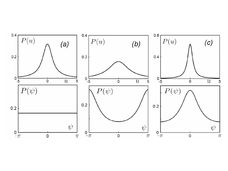
Figure 2: The change of the distribution $P(\psi)$ in the result of the scale transformation of the function $P(u)$, if the form of the latter corresponds to the random phase approximation

For $s=\kappa/k$ one has equality $\tilde{a}=-\tilde{b}$, and factors $\kappa/k$ and $s^{-1}$ compensate each other, so

$$\Delta\left\langle\sin{\psi}\right\rangle_{a,b}=\delta\cdot\left\langle\sin{\psi}\right\rangle_{nat}$$

and we have established invariance of all combinations entering the expressions (25,26) for $D$ and $v$.

6. Conclusion

In the present paper we have derived the equation for the stationary distribution of the phase variable $\psi$, which determinate the parameters of the limiting distribution (5) for $P(\rho)$, and establish independence of these parameters on the boundary conditions, as a consequence of the transformation properties of the equation for $P(\psi)$.

In the result of the present analysis we come to a very simple picture. The phase $\psi$ appears to be a ”bad” variable, while the ”correct” variable is $u={\rm tg}\,\psi/2$. The form of the distribution $P(u)$ is determined by the internal properties of the system and allows sufficiently strong variations for the radical change of parameters in the limiting distribution (5) as a function of the Fermi level (Fig.1). Variation of properies of the ideal leads, attached to the system, results in the scale transformation of the function $P(u)$, which does not affect the values of parameters $v$ and $D$ due to specific properties of equation (33).

On the qualitative level, variations of the distribution $P(\psi)$ in the result of the scale transformations of $P(u)$ are easily predictive and are illustrated in Fig.2. The distribution $P(\psi)$ is uniform, if $P(u)$ has a form $(1/\pi)(1+u^{2})^{-1}$ (Fig.2,a), which is valid in the deep of the allowed band ($\delta\gg\epsilon^{2}$) for the ”natural” ideal leads ($\kappa^{2}=-k^{2}$) and follows from equation (33) for $a=b$ in the main order in $\epsilon^{2}/\delta$. Widening of the distribution $P(u)$ leads to localization of $P(\psi)$ near the edges of the interval $(-\pi,\pi)$ (Fig.2,b), while narrowing leads to localization of $P(\psi)$ in the middle of the interval $(-\pi,\pi)$. (Fig.2,c). However, the rough visual form of the distribution $P(\psi)$ is not physically substantial due to invariance of parameters $v$ and $D$ respective the changes shown in Fig.2.

The discussed problems are not restricted by 1D systems, and analogous difficulties arise in the studies of the Lyapunov exponents in the framework of the generalized version [17] of the Dorokhov–Mello–Pereyra-Kumar equation [18, 19]. The minimal Lyapunov exponent determinates the critical properties of the Anderson transition (it is clear from the well-known numerical algorithm, see references in [17]), and the analogous hidden symmetry can be essential in the studies of the latter.

References

• [1] P. W. Anderson, D. J. Thouless, E. Abrahams, D. S. Fisher, Phys. Rev. B 22, 3519 (1980).
• [2] R. Landauer, IBM J. Res. Dev. 1, 223 (1957); Phil. Mag. 21, 863 (1970); Z. Phys. 68, 217 (1987).
• [3] V. I. Melnikov, Sov. Phys. Sol. St. 23, 444 (1981).
• [4] A. A. Abrikosov, Sol. St. Comm. 37, 997 (1981).
• [5] N. Kumar, Phys. Rev. B 31, 5513 (1985).
• [6] B. Shapiro, Phys. Rev. B 34, 4394 (1986).
• [7] P. Mello, Phys. Rev. B 35, 1082 (1987).
• [8] B. Shapiro, Phil. Mag. 56, 1031 (1987).
• [9] I. M. Suslov, J. Exp. Theor. Phys. 124, 763 (2017) [Zh. Eksp. Teor. Fiz. 151, 897 (2017)].
• [10] I. M. Lifshitz, S. A. Gredeskul, L. A. Pastur, Introduction to the Theory of Disordered Systems, Nauka, Moscow, 1982.
• [11] C. W. J. Beenakker, Rev. Mod. Phys. 69, 731 (1997).
• [12] X. Chang, X. Ma, M. Yepez, A. Z. Genack, P. A. Mello, Phys. Rev. B 96, 180203 (2017).
• [13] L. I. Deych, D. Zaslavsky, A. A. Lisyansky, Phys. Rev. Lett. 81, 5390 (1998).
• [14] L. I. Deych, A. A. Lisyansky, B. L Altshuler, Phys. Rev. Lett. 84, 2678 (2000); Phys. Rev. B 64, 224202 (2001).
• [15] L. I. Deych, M. V. Erementchouk, A. A. Lisyansky, Phys. Rev. Lett. 90, 126601 (2001).
• [16] I. M. Suslov, J. Exp. Theor. Phys. 129, 877 (2019) [Zh. Eksp. Teor. Fiz. 156, 950 (2019)].
• [17] I. M. Suslov, J. Exp. Theor. Phys. 127, 131 (2018) [Zh. Eksp. Teor. Fiz. 154, 152 (2018)].
• [18] O. N. Dorokhov, JETP Letters 36, 318 (1982).
• [19] P. A. Mello, P. Pereyra, N. Kumar, Ann. Phys. (N.Y.) 181, 290 (1988).