Laughlin’s topological charge pump in an atomic Hall cylinder
Abstract
The quantum Hall effect occuring in two-dimensional electron gases was first explained by Laughlin, who envisioned a thought experiment that laid the groundwork for our understanding of topological quantum matter. His proposal is based on a quantum Hall cylinder periodically driven by an axial magnetic field, resulting in the quantized motion of electrons. We realize this milestone experiment with an ultracold gas of dysprosium atoms, the cyclic dimension being encoded in the electronic spin and the axial field controlled by the phases of laser-induced spin-orbit couplings. Our experiment provides a straightforward manifestation of the non-trivial topology of quantum Hall insulators, and could be generalized to strongly-correlated topological systems.
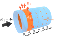
The quantization of Hall conductance observed in two-dimensional electronic systems subjected to a perpendicular magnetic field [1] is intimately linked to the non-trivial topology of Bloch bands [2] and the occurence of chiral edge modes protected from backscattering [3]. The first step in its undertanding was provided by Laughlin, who gave an elegant argument by considering a Hall system in a cylindrical geometry (Fig. 1) [4]. Besides the radial magnetic field yielding the Hall effect, this geometry authorizes an axial field , which does not pierce the surface but threads the cylinder with a flux . Varying the flux controls a quantized electronic motion along the tube, which is directly linked to the underlying band topology. Such quantization of transport was later generalized by Thouless to any physical system subjected to a slow periodic deformation [5], as implemented in electronic quantum dots [6, 7], photonic waveguides [8] and ultracold atomic gases [9, 10].
So far, the topology of magnetic Bloch bands has been revealed in planar systems only, by measuring the quantization of transverse response [1, 11, 12, 13] or observing chiral ballistic edge modes [14, 15, 16]. The realization of Laughlin’s pump experiment requires engineering periodic boundary conditions, which is challenging when using genuine spatial dimensions. The concept of a synthetic dimension encoded in an internal degree of freedom provides an interesting alternative [17, 18, 19], which recently led to the realization of synthetic Hall cylinders [20, 21, 22].
In this work, we use an ultracold gas of 162Dy atoms to engineer a Hall cylinder whose azimuthal coordinate is encoded in the electronic spin [23]. We manipulate the spin using coherent optical transitions, such that a triplet of internal states coupled in a cyclic manner emerges at low energy, leading to an effective cylindrical geometry [24]. The exchange of momentum between light and atoms leads to a spin-orbit coupling that mimics a radial magnetic field [25]. The phases of the laser electric fields also control an effective axial field , which we use to implement Laughlin’s thought experiment and reveal the underlying topology. The topological character of the ground Bloch band manifests as well in a complementary pump experiment driven by Bloch oscillations.
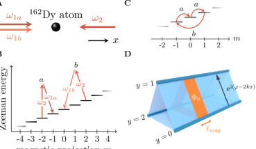
In our experimental protocol, we apply a magnetic field in order to lift the degeneracy between the magnetic sub-levels (with and integer ). Spin transitions of first and second order, i.e. and , are induced by resonant two-photon optical transitions, using a pair of laser beams counter-propagating along (Fig. 2A) [26]. The configuration of laser frequencies is chosen such that the atoms undergo a momentum kick upon either resonant process or shown in Fig. 2B. Here, is the photon momentum for the laser wavelength . The resulting spin-orbit coupling breaks continuous translation symmetry, but conserves the quasi-momentum , defined over the magnetic Brillouin zone , where and are the atomic mass and velocity. The atom dynamics is described by the Hamiltonian
| (1) | ||||
| (2) |
where and are the spin ladder operators, and are the strengths of the first and second-order transitions. The phase difference can be gauged away using a suitable spin rotation, such that we retain hereafter a single phase .
The combination of the two types of transitions induces non-trivial 3-cycles (Fig. 2B), with chiral dynamics in the cyclic variable – each step increasing by one unit. As explained in [24], one expects the emergence of a closed subsystem at low energy, spanned by three spin states , with and where expands on projection states with only. The states will be interpreted in the following as position eigenstates along a cyclic synthetic dimension of length . The operator involved in the spin coupling (2) then acts as a translation , with a hopping amplitude . The low-energy spin dynamics is described by the effective potential
| (3) |
Together with the kinetic energy , it describes the motion of a particle on a cylinder discretized along its circumference (see Fig. 2C). The complex phase mimics the Aharonov-Bohm phase associated with a radial magnetic field (assuming a particle charge ). It defines a magnetic length , such that the magnetic flux through a portion of cylinder of length equals the flux quantum .
Experimentally, we use a gas of about atoms, initially prepared at a temperature , such that the thermal momentum width is much smaller than the Brillouin zone extent, and interaction effects can be neglected on the timescale of our experiments. The atoms are adiabatically loaded in the ground Bloch band by ramping the light coupling parameters, and the mean quasi-momentum is controlled by applying a weak force after the loading (see the Supplementary Materials [26]). We simultaneously probe the distribution of velocity and spin projection . For this, we measure the atom distribution after time-of-flight in the presence of a magnetic field gradient, which separates the different magnetic sub-levels. A typical spin-resolved velocity distribution is shown in Fig. 3A.
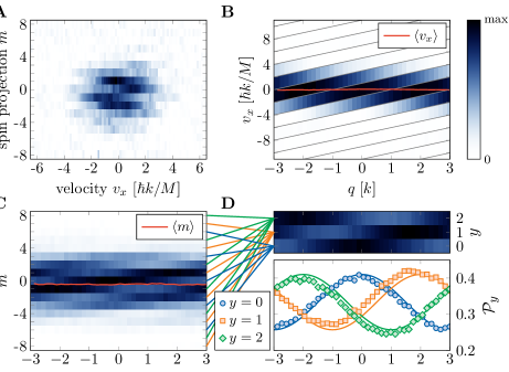
The velocity distribution, plotted in Fig. 3B as a function of , exhibits a period , similar to the case of a simple -lattice. The mean velocity , shown as a red line, remains close to zero. Since it is linked to the slope of the ground-band energy , this shows that the band is quasi-flat. In fact, the band’s flatness in protected from pertubations, such as external magnetic field fluctuations, by the zero net magnetization of the spin states – a similar effect has been used in another implementation of a Hall cylinder using dynamical decoupling techniques [22].
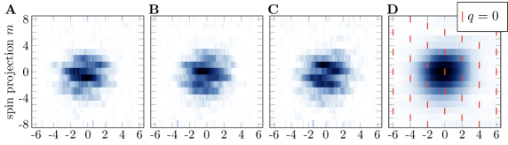
The probabilities of projection on each sub-level reveal a longer periodicity (Fig. 3C), corresponding to the full extent of the magnetic Brillouin zone. It experimentally confirms the spatial separation of magnetic orbitals introduced above. The measurements also give access to the probabilities of projection on the synthetic coordinate , by summing the ’s with (Fig. 3D). The -variation of these distributions reveals a chirality typical of the Hall effect: when increasing the momentum by , the distributions cycle along the synthetic dimension in a directional manner, as [27, 28]. We stress that such a drift does not occur on the mean spin projection , which remains close to zero (red line in Fig. 3C).
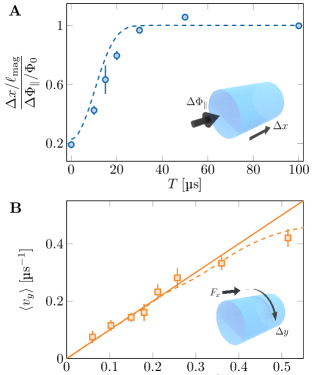
The adiabatic -drift occuring during Bloch oscillations provides a first insight into the topological character of the lowest energy band – similar to the quantized flow of Wannier function charge centers in Chern insulators [29]. To quantify this drift, we cannot rely on the mean position, which is ill-defined for a cyclic dimension [30]. Instead, it is reconstructed by integrating the anomalous velocity induced by the force driving the Bloch oscillation. For this purpose, we conduct a separate experiment, in which we suddenly switch off the force , such that the center-of-mass undergoes a cyclotron oscillation, with the - and -velocities oscillating in quadrature. More precisely, the rate of change of the -velocity gives access to the -velocity, via the exact relation
Hence, the velocity induced by the force is given by the initial slope of (Fig. 4B).
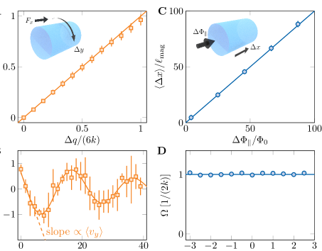
The center-of-mass drift , obtained upon integration of is shown in Fig. 4A. We find that it varies linearly with the quasi-momentum variation (Fig. 4A), such that the drift per Bloch oscillation cycle reads
| (4) |
consistent with a unit winding around the cylinder of circumference [26]. The rotation along occuring over a Bloch oscillation cycle is thus quantized, providing a first manifestation of the non-trivial band topology.
We now characterize the global band topology by implementing Laughlin’s charge pump experiment, and extend the protocol to reveal the local geometrical properties. To simulate the axial magnetic field used to drive the pump, we interpret the complex phase involved in the -hoppings (see equation 3) as the Peierls phase associated with the field threading the cylinder with a flux
| (5) |
We vary by adjusting the phase difference between the laser electric fields involved in the spin transitions.
We drive the pump by slowly ramping the phase , and measure the induced shift of the center-of-mass along the real dimension . The experiment is performed for various values of the quasi-momentum uniformly spanning the magnetic Brillouin zone. The -averaged drift, shown in Fig. 4C, is consistent with a linear variation
in agreement with the expected quantization of transport by the Chern number . The pump adiabaticity is checked by repeating the experiment for various speeds of the flux ramp, and measuring identical responses for slow enough ramps [26].
Our experiments also give access to the anomalous drift of individual momentum states , proportional to the Berry curvature that quantifies the local geometrical properties of quantum states [31]. As shown in Fig. 4D, the measured Berry curvature is flat within error bars, consistent with theory, which predicts with negligible variation. The flatness of the Berry curvature is a consequence of the continuous translation symmetry along , making our system similar to continuous two-dimensional systems with flat Landau levels. In contrast, discrete lattice systems, such as Hofsdtater and Haldane models [32, 33], or previous implementations of synthetic Hall cylinders [20, 21, 22], exhibit dispersive bands with inhomogeneous Berry curvatures.
We have shown that implementing a quantum Hall cylinder gives direct access to the underlying topology of Bloch bands. Our realization of Laughlin’s pump protocol could be generalized to interacting atomic systems, which are expected to form strongly correlated topological states of matter at low temperature. In particular, at fractional fillings, one expects the occurrence of charge density waves as one-dimensional precursors of two-dimensional fractional quantum Hall states [34]. The pumped charge would then be quantized to a rational value, revealing the charge fractionnalization of elementary excitations [35].
References
- v. Klitzing et al. [1980] K. v. Klitzing, G. Dorda, and M. Pepper, New Method for High-Accuracy Determination of the Fine-Structure Constant Based on Quantized Hall Resistance, Phys. Rev. Lett. 45, 494 (1980).
- Thouless et al. [1982] D. J. Thouless, M. Kohmoto, M. P. Nightingale, and M. den Nijs, Quantized Hall Conductance in a Two-Dimensional Periodic Potential, Phys. Rev. Lett. 49, 405 (1982).
- Halperin [1982] B. I. Halperin, Quantized Hall conductance, current-carrying edge states, and the existence of extended states in a two-dimensional disordered potential, Phys. Rev. B 25, 2185 (1982).
- Laughlin [1981] R. B. Laughlin, Quantized Hall conductivity in two dimensions, Phys. Rev. B 23, 5632 (1981).
- Thouless [1983] D. J. Thouless, Quantization of particle transport, Phys. Rev. B 27, 6083 (1983).
- Switkes et al. [1999] M. Switkes, C. M. Marcus, K. Campman, and A. C. Gossard, An Adiabatic Quantum Electron Pump, Science 283, 1905 (1999).
- Watson et al. [2003] S. K. Watson, R. M. Potok, C. M. Marcus, and V. Umansky, Experimental Realization of a Quantum Spin Pump, Phys. Rev. Lett. 91, 258301 (2003).
- Kraus et al. [2012] Y. E. Kraus, Y. Lahini, Z. Ringel, M. Verbin, and O. Zilberberg, Topological States and Adiabatic Pumping in Quasicrystals, Phys. Rev. Lett. 109, 106402 (2012).
- Lohse et al. [2016] M. Lohse, C. Schweizer, O. Zilberberg, M. Aidelsburger, and I. Bloch, A Thouless quantum pump with ultracold bosonic atoms in an optical superlattice, Nat. Phys. 12, 350 (2016).
- Nakajima et al. [2016] S. Nakajima, T. Tomita, S. Taie, T. Ichinose, H. Ozawa, L. Wang, M. Troyer, and Y. Takahashi, Topological Thouless pumping of ultracold fermions, Nat. Phys. 12, 296 (2016).
- Dean et al. [2013] C. R. Dean, L. Wang, P. Maher, C. Forsythe, F. Ghahari, Y. Gao, J. Katoch, M. Ishigami, P. Moon, M. Koshino, T. Taniguchi, K. Watanabe, K. L. Shepard, J. Hone, and P. Kim, Hofstadter’s butterfly and the fractal quantum Hall effect in moiré superlattices, Nature 497, 598 (2013).
- Ponomarenko et al. [2013] L. A. Ponomarenko, R. V. Gorbachev, G. L. Yu, D. C. Elias, R. Jalil, A. A. Patel, A. Mishchenko, A. S. Mayorov, C. R. Woods, J. R. Wallbank, M. Mucha-Kruczynski, B. A. Piot, M. Potemski, I. V. Grigorieva, K. S. Novoselov, F. Guinea, V. I. Fal’ko, and A. K. Geim, Cloning of Dirac fermions in graphene superlattices, Nature 497, 594 (2013).
- Aidelsburger et al. [2015] M. Aidelsburger, M. Lohse, C. Schweizer, M. Atala, J. T. Barreiro, S. Nascimbene, N. Cooper, I. Bloch, and N. Goldman, Measuring the Chern number of Hofstadter bands with ultracold bosonic atoms, Nat. Phys. 11, 162 (2015).
- Wang et al. [2009] Z. Wang, Y. Chong, J. D. Joannopoulos, and M. Soljačić, Observation of unidirectional backscattering-immune topological electromagnetic states, Nature 461, 772 (2009).
- Hafezi et al. [2013] M. Hafezi, S. Mittal, J. Fan, A. Migdall, and J. Taylor, Imaging topological edge states in silicon photonics, Nat. Photonics 7, 1001 (2013).
- Rechtsman et al. [2013] M. C. Rechtsman, J. M. Zeuner, Y. Plotnik, Y. Lumer, D. Podolsky, F. Dreisow, S. Nolte, M. Segev, and A. Szameit, Photonic Floquet topological insulators, Nature 496, 196 (2013).
- Celi et al. [2014] A. Celi, P. Massignan, J. Ruseckas, N. Goldman, I. B. Spielman, G. Juzeliūnas, and M. Lewenstein, Synthetic Gauge Fields in Synthetic Dimensions, Phys. Rev. Lett. 112 (2014).
- Mancini et al. [2015] M. Mancini, G. Pagano, G. Cappellini, L. Livi, M. Rider, J. Catani, C. Sias, P. Zoller, M. Inguscio, M. Dalmonte, and L. Fallani, Observation of chiral edge states with neutral fermions in synthetic Hall ribbons, Science 349, 1510 (2015).
- Stuhl et al. [2015] B. K. Stuhl, H.-I. Lu, L. M. Aycock, D. Genkina, and I. B. Spielman, Visualizing edge states with an atomic Bose gas in the quantum Hall regime, Science 349, 1514 (2015).
- Han et al. [2019] J. H. Han, J. H. Kang, and Y. Shin, Band Gap Closing in a Synthetic Hall Tube of Neutral Fermions, Phys. Rev. Lett. 122, 065303 (2019).
- Li et al. [2018] C.-H. Li, Y. Yan, S. Choudhury, D. B. Blasing, Q. Zhou, and Y. P. Chen, A Bose-Einstein condensate on a synthetic Hall cylinder, arXiv:1809.02122 (2018).
- Liang et al. [2021] Q.-Y. Liang, D. Trypogeorgos, A. Valdés-Curiel, J. Tao, M. Zhao, and I. B. Spielman, Coherence and decoherence in the Harper-Hofstadter model, Phys. Rev. Research 3, 023058 (2021).
- Chalopin et al. [2020] T. Chalopin, T. Satoor, A. Evrard, V. Makhalov, J. Dalibard, R. Lopes, and S. Nascimbene, Probing chiral edge dynamics and bulk topology of a synthetic Hall system, Nat. Phys. 16, 1017 (2020).
- Fabre et al. [2021] A. Fabre, J.-B. Bouhiron, T. Satoor, R. Lopes, and S. Nascimbene, Simulating two-dimensional dynamics within a large-size atomic spin, arXiv:2110.05269 (2021).
- Dalibard et al. [2011] J. Dalibard, F. Gerbier, G. Juzeliūnas, and P. Öhberg, Colloquium : Artificial gauge potentials for neutral atoms, Rev. Mod. Phys. 83, 1523 (2011).
- [26] Materials and methods are available as supplementary materials.
- Yan et al. [2018] Y. Yan, S.-L. Zhang, S. Choudhury, and Q. Zhou, Emergent periodic and quasiperiodic lattices on surfaces of synthetic Hall tori and synthetic Hall cylinders, arXiv:1810.12331 (2018).
- Anderson et al. [2020] R. P. Anderson, D. Trypogeorgos, A. Valdés-Curiel, Q.-Y. Liang, J. Tao, M. Zhao, T. Andrijauskas, G. Juzeliūnas, and I. B. Spielman, Realization of a deeply subwavelength adiabatic optical lattice, Phys. Rev. Research 2, 013149 (2020).
- Taherinejad et al. [2014] M. Taherinejad, K. F. Garrity, and D. Vanderbilt, Wannier center sheets in topological insulators, Phys. Rev. B 89, 115102 (2014).
- Lynch [1995] R. Lynch, The quantum phase problem: A critical review, Physics Reports 256, 367 (1995).
- Lu et al. [2016] H.-I. Lu, M. Schemmer, L. M. Aycock, D. Genkina, S. Sugawa, and I. B. Spielman, Geometrical Pumping with a Bose-Einstein Condensate, Phys. Rev. Lett. 116, 200402 (2016).
- Hofstadter [1976] D. R. Hofstadter, Energy levels and wave functions of Bloch electrons in rational and irrational magnetic fields, Phys. Rev. B 14, 2239 (1976).
- Haldane [1988] F. D. M. Haldane, Model for a Quantum Hall Effect without Landau Levels: Condensed-Matter Realization of the ”Parity Anomaly”, Phys. Rev. Lett. 61, 2015 (1988).
- Tao and Thouless [1983] R. Tao and D. J. Thouless, Fractional quantization of Hall conductance, Phys. Rev. B 28, 1142 (1983).
- Laughlin [1999] R. B. Laughlin, Nobel lecture: Fractional quantization, Rev. Mod. Phys. 71, 863 (1999).
- Cohen-Tannoudji and Dupont-Roc [1972] C. Cohen-Tannoudji and J. Dupont-Roc, Experimental Study of Zeeman Light Shifts in Weak Magnetic Fields, Phys. Rev. A 5, 968 (1972).
- Luo et al. [2020] X.-W. Luo, J. Zhang, and C. Zhang, Tunable flux through a synthetic Hall tube of neutral fermions, Phys. Rev. A 102, 063327 (2020).
Acknowledgments
We thank Jean Dalibard for insightful discussions and careful reading of the manuscript, and Thomas Chalopin for discussions at an early stage of this work. Funding: This work is supported by European Union (grant TOPODY 756722 from the European Research Council). Author contributions: A.F., J.B.B. and T.S. carried out the experiments, supervised by R.L. and S.N. All authors were involved in the data analysis and contributed to the manuscript.
Materials and methods
I Implementation of spin couplings
To implement the spin-orbit coupling, we apply a magnetic field along that induces a Zeeman splitting between the successive magnetic levels . The spin dynamics is driven by two-photon optical transitions, using a pair of laser beams as shown in Fig. 2A. Each beam is linearly polarized, along and for the laser beams 1 and 2, which propagate along and , respectively. Their waist is much larger than the rms size of the atomic gas, such that the light intensity can be considered uniform.
The laser frequencies are set close to the atomic resonance of wavelength (red detuning from resonance ), coupling the electronic ground state of angular momentum to an excited level with . The proximity to an isolated optical transition leads to spin-dependent light shifts, which we use here to induce resonant spin transitions. Each beam produces a quadratic energy shift of the magnetic sub-levels proportional to [36], which we cancel by setting the polarization angle to .
In order to induce the first- and second-order spin transitions, the laser 2 is monochromatic at frequency , while the laser 1 has two frequency components and (Fig. 2A). The component is set close to , leading to the process () that drives a spin transition while imparting a velocity recoil , where is the one-photon recoil velocity. The other frequency component is close to , inducing the second process () with a spin transition and a recoil (Fig. 2B). Our experiments are performed with spin coupling amplitudes and .
II Band structure and topology
II.1 Band structure
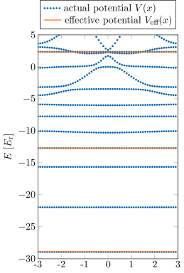
We show in Fig. S1 the structure of magnetic Bloch bands calculated for the couplings and used in our experiment, with either the actual potential or the effective potential involving the three spin states only. The band structure of the effective model matches well several bands of , including the ground band. The bands that are not reproduced correspond to excitations of the system outside the three spin states. They manifest the existence of an additional degree of freedom aside from the and dynamics, which could be used in future experiments to engineer more complex topological systems [24]. This degree of freedom remains frozen in our experiments, and it plays no role in the interpretation of our results.
II.2 Topological character of the ground band
We recall the expression of the Hamiltonian
| (S1) | ||||
| (S2) |
describing the atom dynamics. The quasi-momentum being a conserved quantity, the dynamics can be reduced to a Hamiltonian parametrized by the couple , which varies on the torus and . The topological character of the ground band is determined by the value of the Chern number [2, 37]
where we introduce the Berry curvature
with the velocities and , and we introduce the Bloch state of the band , of energy . The ground band corresponds to the index . In our system, Bloch states of the same band and quasi-momentum , but different , can be mapped on each other by a spatial translation. Hence, they share the same Berry curvature, which thus only depends on . Integrating over , we get the relation used in the main text
For the couplings and used in the experiment, the Berry curvature is extremely flat, equal to for all momenta with a relative variation less than . Its integral over the Brillouin zone yields a Chern number .
III Loading of the ground band
III.1 Control of the Zeeman field and quasi-momentum
The preparation of Bloch states of the ground band with a given quasi-momentum uses additional control parameters provided by setting the laser frequencies away from the Zeeman resonance conditions. We define the detunings and . The time dependency of the Hamiltonian can be suppressed with the right choice of transformations. First, we consider the atom motion in a reference frame moving at velocity with respect to the laboratory frame. Second, we apply a gauge transform defined by the unitary operator with . Using the rotating wave approximation to suppress fast-oscillating terms, we obtain a static Hamiltonian
| (S3) |
where is defined in (2) in the main text and plays the role of a Zeeman field. When is set to zero, this Hamiltonian reduces to the one considered in the main text, given by (1). A time-dependent frame velocity results in an inertial force along the real dimension , which we use to drive Bloch oscillations in our system.
III.2 Protocol for the ground-band loading
The preparation of the ground state of the Hamiltonian (1) with and is realized as follows. We set the initial laser frequencies such that the frame velocity cancels, and the Zeeman field is set to . This value is large enough to ensure that the gas is almost fully polarized in . The atoms have a zero mean velocity , such that the mean quasi-momentum reads .
To load the ground band of the desired Hamiltonian with , we first increase the light intensities to their final values in . We then ramp the Zeeman field towards zero in . This ramp duration is a compromise to ensure adiabaticity while minimizing spin-changing collisions occuring on the timescale of a few milliseconds. The minimum value of the gap to the first excited band sets the timescale for adiabaticity , much shorter that the chosen ramp duration. We confirm the ramp adiabaticity using a numerical simulation of the atom dynamics, which predicts an overlap with the ground band after the ramp above 97%.
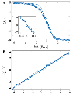
The adiabatic loading is checked by probing the system as a function of . For , we expect the system to exhibit a non-zero magnetization . Its measurement, shown in Fig. S2A, agrees well with theory.
The final step in the state preparation is the application of a force to induce Bloch oscillations. The mean quasi-momentum evolves as , which we use to prepare the desired quasi-momentum state. We show in Fig. S2B the measured values of quasi-momentum during a Bloch oscillation, which agrees well with the expected variation. Bloch oscillations are also used to study the topological Hall response, by measuring the velocity along the synthetic dimension induced by the force (see main text).
IV Characterization of the ground band
The study of the ground band properties are based on the measurement of spin-resolved velocity distributions. For a Bloch state of quasi-momentum , the velocity takes discrete values only, at
| (S4) |
In our system, the thermal broadening of momentum leads to a continuous velocity distribution (Fig. S3A,B,C). Importantly, the equation (S4) shows that different quasi-momentum states contribute to distinct velocities in the spin-resolved velocity distribution. The thermal broadening can thus be deconvolved, leading to the velocity and spin distributions resolved in quasi-momentum shown in Fig. 3B,C. In practice, in order to treat all quasi-momenta on equal footing, we first average the spin-resolved velocity distributions measured for various values of uniformly spanning the first Brillouin zone. We then deconvolve the data by selecting the velocity components of a given from the averaged distribution, according to (S4) (Fig. S3D).
V Transverse response in Bloch oscillation experiments
We discuss in the main text the adiabatic -drift occuring during a Bloch oscillation driven by a force . In the weak force limit, one expects the mean velocity to be proportional to the force and to the Berry curvature , as
| (S5) |
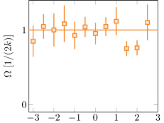
We show in Fig. S4 the measured Berry curvature for various values of the mean quasi-momentum . The measurements are consistent with a flat Berry curvature – similar to the measurements with the Laughlin pump protocol, albeit with larger error bars here due to the differentiation operation used to extract the velocity from the -velocity oscillations (Fig. 4B). The adiabaticity criterion required for the linear relation (S5) to apply is discussed in section VI.2.
The adiabatic -drift acquired for a duration reads
| (S6) | ||||
| (S7) |
where we used . The drift accumulated over a period thus reads
| (S8) | ||||
| (S9) |
where is the Chern number. This expression links the quantization of the rotation along during a Bloch oscillation to the Chern number characterizing the ground-band topology.
VI Adiabaticity of topological pumps
The quantization of topological pumps requires the pump control parameters to be varied adiabatically. We present here a study of adiabaticity of the two topological pumps considered in the main text.
VI.1 Laughlin pump adiabaticity
The Laughlin pump is driven by inserting a longitudinal magnetic flux . The flux is increased linearly in time at a rate , after a ramp-up phase of the rate using an s-shaped profile of duration . We show in Fig. S5A the mean atom displacement as a function of the ramp time . For slow ramps , the displacement is compatible with the value given by the Berry curvature . Deviations are observed for faster ramps in agreement with a numerical simulation of the atom dynamics. The measurements shown in Fig. 4A are performed with a ramp duration in the adiabatic regime.
VI.2 Bloch oscillation adiabaticity
The other topological pump studied in our work consists in the motion along the synthetic dimension induced by a force along the real dimension . We show in Fig. S5B the mean velocity as a function of . For , the -velocity varies linearly with , in agreement with the expected adiabatic response. The deviations observed for larger forces are well accounted for by a numerical simulation of the atom dynamics. The measurements shown in Fig. 4B use a force , well in the adiabatic regime.
VII Bandgap measurements
We studied the low-energy excitations of the system, which are of two types: the excitations described by the effective Hall cylinder model, which assume the spin state to remain in the 3-dimensional manifold, and the excitations leaving this subspace.
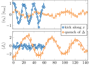
In order to probe excitations of the effective Hall cylinder model, we apply a kick along using a short pulse of the force , which does not affect the spin degree of freedom. As shown in Fig. S6, we measure an oscillation of the mean velocity , associated to an energy gap of , close to the expected value of (corresponding to the gap to the third excited band of the full model, see Fig. S1). During this evolution, the magnetization remains close to zero, as expected for an excitation within the spin states.
We also studied the excitation to the first excited band, which involves spin states outside the manifold. To promote the system to this band, we prepare the ground state with a non-zero Zeeman field , such that the system exhibits a non-zero magnetization . We then quench the Zeeman field to zero, and measure the subsequent evolution of the -velocity and magnetization. We measure an oscillation of the magnetization with a longer period, corresponding to a gap of , close to the expected value of .