Sparsity-Specific Code Optimization using Expression Trees

Abstract.

We introduce a code generator that converts unoptimized C++ code operating on sparse data into vectorized and parallel CPU or GPU kernels. Our approach unrolls the computation into a massive expression graph, performs redundant expression elimination, grouping, and then generates an architecture-specific kernel to solve the same problem, assuming that the sparsity pattern is fixed, which is a common scenario in many applications in computer graphics and scientific computing. We show that our approach scales to large problems and can achieve speedups of two orders of magnitude on CPUs and three orders of magnitude on GPUs, compared to a set of manually optimized CPU baselines. To demonstrate the practical applicability of our approach, we employ it to optimize popular algorithms with applications to physical simulation and interactive mesh deformation.

1. Introduction

The optimization of numerical code using combinations of algorithmic improvements and custom hardware played a core role in advancing computer graphics, enabling the move from the early days of rasterizing individual polygons in seconds to the modern era of raytracing entire scenes at interactive rates. With manufacturers building more specialized processors and increased parallelism in hardware, the path to optimizing code for a specific processor is becoming more complex.

In this work we focus on optimizing numerical code that is dominated by sparse operations. Algorithms in computer graphics, and geometry processing in particular, make heavy use of sparse matrices or can be easily formulated as operations on them. A reason for this fact is that we often study how global behavior of a system emerges from local interactions, which are inherently sparse. This observation generalizes to adjacent disciplines like finite element analysis in engineering and computer vision.

Arithmetic operations between sparse matrices can be quite costly and hard to optimize. In contrast to their dense counterparts, they cannot easily benefit from highly optimized BLAS or LAPACK dense matrix routines. Recent implementations (Intel, 2021; Nvidia, 2020; AMD, 2020) of sparse matrix operations, like the sparse matrix-matrix product, enable analyzing the sparsity structure of specific operands and the result in order to schedule an optimized parallel computation plan and preallocate memory. Executing this plan computes these operations efficiently as long as the sparsity structure does not change. Unfortunately, these optimized implementations are very limited. Nvidia’s cuSparse (Nvidia, 2020), for example, only supports products of sparse matrix in row-major format and does not allow implicitly transposing one of the factors. Sparse matrix addition is not supported directly; only accumulation of sparse matrix products of the same structure is possible. Even more restricting is the fact that compound operations are generally not supported. For example, the computation pattern for the operation $\mathbf{L}\mathbf{M}\mathbf{L}^{\top}+\mathbf{A}$, where all operators are sparse matrices, is also fixed but must be broken down into individual operations for the pre-analysis approach.

We take the idea of pre-analysis a step further and analyze full sparse expressions. We assume that we have a set of (sparse) input matrices that are combined to form an output matrix. Our method is not limited to a fixed set of arithmetic operations but allows for arbitrary manipulations and storage formats as long as they are implemented in C++ code. We build on ideas recently introduced with the EGGS system (Tang et al., 2020b). Like EGGS, we represent all values of the output matrix as expression trees encoding all operations necessary to compute the output values from the input values. We decompose, group, and optimize these expression trees to generate code that efficiently evaluates all trees. Our generated programs utilize expression unrolling, vectorization, parallelization, and regular memory accesses, both on CPU and GPU, to achieve 1–3 orders of magnitude in performance increase.

We extend EGGS in several ways. Instead of operating on entire output expression trees individually, we optimize complex sparse operations by operating on subtrees of finer granularity. This allows us to optimize a spectrum of applications where EGGS would fail to produce faster code. Additionally, we target GPUs and introduce several new optimization steps, including optimizing for coalesced memory accesses and aligned memory reads.

We additionally support sparse matrix construction. Assembling sparse matrices from individual entries can take a significant amount of time, sometimes even dominating linear system solves in finite element based simulations. In the context of physical simulation, for example, the current state of a simulation is characterized by position and velocity data. Our method can generate code that takes these values as input and constructs the final sparse system matrix in one step. In many cases, the sparse matrix is the Hessian of a non-linear energy, for example when employing Newton’s method. Our system supports constructing the Hessian directly from an energy formulation using symbolic automatic differentiation. We show that code generated by automatic differentiation is as efficient as code generated from a hand optimized implementation of the Hessian.

Storing runtime information in the form of expression trees allows us to generate fine tuned code; however, this approach comes with some disadvantages. A central limitation is the focus on static expressions which means that we have only limited support for branching based on non-constant numerical values. Moreover, the memory requirements for storing all expressions can be significant. We report peak memory usage of our code generator in Table 3 and demonstrate that our method is still able to scale to typical mesh resolutions. In terms of preprocessing time our system requires up to 30 minutes in extreme cases which makes it useful only if many instances of the code will be executed, for example in a commercial application. We believe that an optimized and parallelized implementation of our pipeline as well as improved expression caching can alleviate these problems. We elaborate on application areas in Section 3.3.

We validate our approach by automatically optimizing the performance of popular computer graphics algorithms, e.g. for mesh deformation (Sorkine and Alexa, 2007) and physical simulation (Baraff and Witkin, 1998), by using our approach on existing code. This automatic optimization only requires minor modifications to the original code in order to apply our approach.

1.1. Contributions

In this paper we present several algorithmic and technical contributions that improve upon EGGS (Tang et al., 2020b). The most important novel features are:

1. Expression decomposition. We introduce advanced expression decomposition (Section 4.2). By breaking down expression trees into smaller expressions that can be cached and reused, we address a central problem of EGGS: the lack of scalability in terms of expression complexity.

2. Memory optimization. We introduce several ways to optimize memory accesses (Section 4.8) and demonstrate their practical utility, especially when targeting GPUs.

3. Code optimization. We present new ways to optimize generated code using expression simplification (Section 4.5) and code transformation to facilitate vectorization (Section 4.8). Moreover, we support code generation for evaluating derivatives.

In an ablation study (Section 5.9) we demonstrate that all contributions cooperatively result in the significant speedups we report. Depending on the example and target device, the effects of individual optimizations vary.

We will publish the code of our system to facilitate further research. We consider our prototype implementation to be a proof of concept demonstrating that it is possible to accelerate a wide range of example programs even with limited scalability in terms of processing time, memory and code characteristics. We discuss those limitations (e.g. Section 3.3, Appendix F) and plan to continue development towards software applicable in even broader scenarios.

2. Related Work

Dense & sparse matrix libraries

Libraries for dense linear algebra (Anderson et al., 1999; Whaley and Dongarra, 1998; Guennebaud et al., 2010; Van Der Walt et al., 2011; Sanderson, 2010; Intel, 2021) have found wide adoption due to their ability to optimize computation using platform-specific code. One of the most popular recent packages is the BLIS (Van Zee and van de Geijn, 2015) library generator, which utilizes the combination of data movement specification and a single kernel definition to generate optimized code for dense matrix multiplication, using the approach by Goto and van de Geijn (2008).

Sparse matrices are increasingly important for applications, often written in languages such as MATLAB (2014), Julia (Bezanson et al., 2012), and with libraries like Eigen (Guennebaud et al., 2010), PETSc (Balay et al., 1997), Blaze (Iglberger et al., 2012), SciPy (Virtanen et al., 2020) and Boost uBLAS (Walter and Koch, 2007). Different libraries support different sparse matrix formats for different subsets of operations, with compressed sparse row/column (CSR/CSC) and coordinate (COO) being most common. For some applications, leveraging blocked structure within the sparse matrix can lead to better performance, as first demonstrated by OSKI and the parallel pOSKI libraries (Vuduc et al., 2005; Byun et al., 2012), which use the block CSR (BCSR) format to reduce memory traffic and better utilize registers. More recently, sparse neural networks (Liu et al., 2015) have made libraries for sparse computations important in machine learning. Tensorflow Sparse (Google, 2017) and TorchSparse (Tang et al., 2020a) introduce optimized sparse computations to existing machine learning frameworks.

Sparse linear algebra compilers

Compilers targeting sparse linear algebra generate customized code based on the linear algebra operation and data structure. Bik and Wijshoff (1993; 1994) and the Bernoulli project (Kotlyar et al., 1997) built compilers for certain sparse operations. More recently, Venkat et al. (2016) utilize the CHiLL polyhedral framework (Venkat et al., 2015) to optimize sparse matrix-vector operations using an inspector-executor approach and the polyhedral model (Feautrier, 1988; Pugh, 1991) to tailor runtime behavior to the specific matrix. The polyhedral model allows for compact representation and optimization of a program without resorting to explicit loop unrolling.

The taco tensor algebra (Kjolstad et al., 2017) compiler generalized previous approaches to sparse code generation to build a compiler that supports a wide variety of tensor formats (Chou et al., 2018) for generating mixed sparse and dense tensor algebra. The compiler has been extended to support Halide-style (Ragan-Kelley et al., 2012, 2013) separation of computation from scheduling, enabling taco to generate optimized code for both CPUs and GPUs (Senanayake et al., 2020). The techniques we present could be used to extend taco to support code generation tailored for specific sparsity patterns.

Sparsity-specific code generation

Prior work has applied polyhedral techniques to generate efficient sparsity-specific code by finding dense substructures within sparse matrices (Augustine et al., 2019) for SpMV. In contrast, our work extends beyond sparse matrix-vector multiplication. Sparsity-specific code generation techniques have also been used to speed up Cholesky factorization and backsolves (Cheshmi et al., 2018); the technique utilized for these solves analyzes dependencies between values in order to create an execution plan, while our technique relies on per-entry expression trees. Finally, while we build upon the CPU-specific code generation demonstrated by EGGS (Tang et al., 2020b), our technique extends and generalizes their approach to support GPUs and includes new optimizations to better utilize memory bandwidth and generate more efficient code. RXMesh (Mahmoud et al., 2021) uses a domain-specific strategy to partition meshes into contiguous patches, allowing GPUs to better utilize coalesced memory accesses. Our strategy optimizes memory access patterns by grouping expressions.

Domain specific languages for simulation & geometry processing

In recent years several domain specific languages (DSLs) for phyiscal simulation and geometry processing have been introduced. Their development is commonly motivated by the idea to separate the implementation of on algorithm operating on a (mesh) graph and its scheduling on a specific device, similar to Halide (Ragan-Kelley et al., 2012) for image processing. Simit (Kjolstad et al., 2016) and Ebb (Bernstein et al., 2016) provide languages that make it convenient to express global energies in terms of local contributions. This approach enables the user to focus on the actual energy formulation and automatically generate correct, efficient code for CPUs or GPUs. The Opt system (Devito et al., 2017) and its recent successor Thallo (Mara et al., 2021) follow a similar route but focus on the class of non-linear least squares problems. These methods can automatically evaluate the required Jacobians and generate complete solvers based on the Gauss-Newton or Levenberg-Marquardt algorithm. These method have a different focus compared to our approach. They strive to make the implementation of specific energies more convenient and focus on the optimization of solvers and very specific sparse operations. The power of these domain specific languages stems from their high level of abstraction making them convenient to use, at the cost of limited generality. Our approach, on the other hand, is agnostic to the fact that there may be an underlying mesh structure, and is potentially complementary to DSLs for specific uses of sparse matrices. The other key difference is that we do not try to generate efficient code for a specific type of optimization problem but rather for a specific problem instance.

3. Overview

Figure 1. Overview of our code optimization technique. Starting from an existing implementation we generate code that is optimized for a specific structure of input values. We target both, CPUs and GPUs.

In this section we first provide background information about concepts introduced in EGGS (Tang et al., 2020b) and used by our system. We then give an overview of the different stages of our method and elaborate on alternative implementation options. Finally we describe the scope of applications that benefit from our approach the most.

3.1. Background

We take C++ code containing algebraic operations on sparse matrices and their construction as input for our method. The operations can be implemented using Eigen (Guennebaud et al., 2010) or any other templated library in combination with custom code. We build upon the basic principles employed in the EGGS system and rely on the concept of expression trees to encode numerical computations. To facilitate the integration of such a system with existing algorithms, both EGGS’ and our approach replace numerical types (e.g., double) with a custom Symbolic class, which uses operator overloading to effectively build an expression tree for every output value, deferring the computations to a later stage. As an example, consider the following code implementing a simple function f:

⬇

Symbolic g(Symbolic a, Symbolic b) {

return a + b;

}

\parSymbolic f(Symbolic a, Symbolic b) {

return 2 * g(a, b) + sqrt(a);

}

Executing it with Symbolic arguments representing the variables a and b will return the expression tree depicted in the inset. If the

function f is part of an existing non templated code base, a minor change of the code is required: template f and g to support execution with floating point as well as with Symbolic arguments. Each instance is either a constant, variable or an operation on a set of child instances. All instances together with their parent/child relationships define a directed acyclic graph (DAG), a data structure commonly used in compiler design (Aho et al., 2013). We differentiate between the concept of expression tree and its efficient encoding as a DAG. Executing the function minipage[c]0.7

⬇

Symbolic h(Symbolic a, Symbolic b) {

x = a * (a + b);

return x * x;

}

Note that the leaf x are only stored once making it easy to identify common subexpressions. The full expression tree is not explicitly represented and would contain individual nodes for these expressions. While the trees of different output values may differ, they commonly share subtrees that have the same structure in the following sense: Two trees are structurally equivalent if they only differ by their leaves but not by the operations required to evaluate them. Consequently, we can compute the two results using the same piece of (optimized) code which we call kernel.

A common source for structurally similar expressions are sparse matrix operations. The inset shows the sparsity pattern of the Laplacian $\mathbf{L}$ of a mesh with 17 vertices. In order to compute the matrix product $\mathbf{L}^{2}=\mathbf{L}^{\top}\mathbf{L}$ efficiently, only the non-zero values of $\mathbf{L}^{2}$ are computed. Computing each element of $\mathbf{L}^{2}$ from the entries $l_{i}$ of $\mathbf{L}$ means evaluating expressions of the form

$$l_{p_{1}}l_{p_{2}}+\cdots+l_{p_{n-1}}l_{p_{n}},$$

where $p_{i}$ is an index referencing a particular entry of the input matrix. Since the matrix inherits its structure from a mesh, the length of these sums differ only within a certain range; in this case $n\in\{6,8,10,12,14,16,18\}$ takes on only 7 different values. Our method will generate code for computing the matrix product by running 7 vectorized kernels in parallel; one for each possible value of $n$. For $n=6$ the code for the kernel will have the following form

⬇

\parx[p[7*i]] = x[p[7*i+1]]*x[p[7*i+2]]

+ x[p[7*i+3]]*x[p[7*i+4]] + x[p[7*i+5]]*x[p[7*i+6]];

\par

This example does not feature any subexpressions that appear multiple times and can be efficiently handled by EGGS as well. The computation of $\mathbf{L}^{3}$, however, is more involved and causes EGGS to fail producing performant code (see Section 5.2) while our method succeeds.

3.2. System overview

A CPU kernel evaluating several instances of structurally equivalent expressions might look like the following code:

⬇

void k(double*x, double* c, int* p) {

for (int i = 0; i < 256; ++i) {

x[p[2*i]] = c[i] * sqrt(x[p[2*i+1]]);

}

}

Each loop iteration evaluates one of the 256 expression trees making up the group. The array c contains the constants. Kernels can significantly benefit from vectorization and parallelization, as we describe in Section 4.8. The goal of our method is to evaluate all expressions of a specific program using a small number of kernels. Since we compile fixed expression trees, our technique is limited in terms of conditional branching if the condition depends on numeric values, as we discuss in Section 4.7. Transforming a given piece of code together with a set of symbolic input and output values into an optimized program requires several steps (Figure 1). To provide an overview, we briefly describe them here and follow up with more details in the next section.

1. Symbolic execution (Section 4.7). The first step executes the code to be compiled. After this phase, each output variable contains an expression tree that can be used to produce the output value for an arbitrary assignment of the input variables. Optionally, we can compute symbolic derivatives for specific expressions (Section 4.9).

2. Expression decomposition (Section 4.2). After the execution phase we end up with a set of expressions. By counting the references to each node and analyzing their complexity we decide which subexpressions should be evaluated independently with their result stored in variables (intermediate expressions)

3. Expression grouping (Section 4.3). All outputs and intermediate expressions are grouped based on their structure. We can evaluate all group members using the same template expression by substituting the correct leaves. Kernels for each group are generated from these expressions. In order to facilitate parallelization no group member can depend on a result of another member. We enforce this property by splitting groups if necessary.

4. Leaf harvesting (Section 4.4). The expressions within a group differ only by their leaves. To identify the leaves, we traverse all group members and store variables and constants in a table with dimensions ‘number of expressions’ $\times$ ‘number of leaves’ for each group.

5. Expression optimization (Section 4.5). The template expression is hierarchically divided into subexpressions, similar to the expression decomposition stage. Each subexpression will be simplified using a set of algebraic simplification rules.

6. Code generation (Section 4.8). The last step produces code for a specific target architecture. To this end, we determine the memory locations to store the values of intermediate variables in order to optimize memory access patterns. The code is optimized for vectorization and parallelization.

3.3. Requirements for input code

Apart from being implemented using templates on the numeric type, an algorithm should posses a few characteristics in order to benefit from our approach.

• 1. Limited conditional branching. Branching should only depend on constant parameters such as matrix dimensions or should be formulated as a conditional assignment (Section 4.7).

• 2. Overhead amortization. Since the goal of our method is to compile code for a specific structure of input data, we will only see a benefit for applications that run enough instances with the same input structure to amortize the initial compilation cost.

• 3. Expression tree variation. The set of expression trees associated with the output values should feature a small set of unique expression tree structures to facilitate single instruction, multiple data (SIMD) parallelism and a small number of kernels.

Several applications in computer graphics, geometry processing, and scientific computing in particular exhibit precisely these properties. For instance, in the minimization of a non-linear energy defined for a mesh, each step of the iterative procedure requires the computation of the current energy value as well as derivative information, namely the gradient and Hessian. Sufficiently smooth energies will have gradients and Hessians expressed with minimal conditional branching. Another common property of energies is that they can be computed as the summations of local interactions between mesh elements in applications like bending, shearing, or stretching. Consequently, the Hessian is not only sparse, but the expression trees of their numeric values produce only a limited number of unique tree topologies based on the vertex degree. These properties make a large class of geometric optimization algorithms perfect candidates for our method. Even if algorithms do not qualify our method might still be applicable. Collision handling in physical simulation, for example, modifies system matrices locally in a way that is unknown at compile time. However, it is in many cases possible to modify a generated system matrix in a preprocess to reflect collision forces. In this situation our method would still optimize the bulk of computation and leave the parts that require conditional branching to the host code. In Section 5 we demonstrate that our approach can be applied to a variety of existing codebases. In the next section, we describe the details of our system.

4. Method

Efficiently handling massive expression trees requires carefully designed algorithms in order to maintain a sufficient degree of scalability. Here we describe the core ideas necessary to implement our method. Throughout we make use of established techiques like directed acyclic graphs and memoization.

4.1. Efficient tree processing

We need to be able to efficiently compare expression trees in terms of their structural and algebraic equivalence. Two trees are structurally equivalent (Section 4.1.1) if they are identical up to their leaves, which may contain different symbolic values or constants. Trees are algebraically equivalent (Section 4.1.2) if they evaluate to the same result. Structurally equivalent trees are algebraically equivalent if their leaves are identical; algebraic equivalent trees do not have to be structurally equivalent. To identify both types of tree equivalence, we leverage a hashing technique that does not require tree traversal. The idea is to compute hashes that only depend on the structure or algebraic equivalence class and identify them uniquely. This can be done by using hash functions generating hashes of sufficient length, like a variant of the secure hash algorithm (SHA), to reduce the collision probability to practically zero. The same concept is used in universally unique identifiers (UUIDs). Our implementation allows to optionally check for hash collisions and we did not find any for 64-bit hashes in our experiments. For other tasks in our pipeline, like dependency detection, tree traversals are not avoidable. In these cases we use selective post- or pre-order tree traversals (Section 4.1.5).

4.1.1. Structural hashing

Name: structureHash(SymbolicExpression x)

Output: Structural hash value for expression x.

if hashIsValid then // return hash if it has been computed. return h else

if Op(x) == Variable then h = variableHash else if Op(x) == Constant then h = constantHash else foreach c in Childs(x) do h = Hash(structureHash(c), h) end foreach

end if

return Hash(Hash(Op(x)), h) end if

ALGORITHM 1 Structure Hashing

To compute hashes identifying the structure of an expression we recursively combine subtree hashes. Algorithm 1 shows an implementation of this idea. The structural hash value of all leaf nodes is one of two fixed hash values: one for variables and one for constants. All other nodes represent arithmetic operations involving one or more child expressions. The function Hash produces a hash value based on its arguments. The structural hash of each expression is computed and stored as soon as the expression is generated. For commutative operations structural hashes are invariant under child permutation because we sort them by hash during construction.

4.1.2. Algebraic hashing

Algebraic hashing works similarly to structural hashing but serves a different purpose. If algebraic hashes of two expression trees are identical, they evaluate to the same numeric value. To this end, we only change the way hashes are computed for leaves. For variables, we compute a hash unique to its variable id. The hash for integer constants is their numerical value. Details and pseudocode can be found in Appendix A. The hash for expressions representing multiplication or addition are the product or sum of their operands. The special rules for commutative operations and constants allow us to identify expressions with vastly different tree structures that evaluate to the same value. For instance, the two expressions

$$2(x+y)(z+w)\quad\text{and}\quad 2xz+(2z+2w)y+xw+wx,$$

will have the same algebraic hash.

4.1.3. DAG compression

Using hashing we can implement memoized constructors. To this end we maintain a map relating hashes to expressions. Whenever a new expression is constructed we first check if an equivalent expression already exists and reuse it if possible.

4.1.4. Expression complexity

When optimizing expression trees, we make decisions based on expression complexity $c$. Whenever we construct an expression, we compute $c$ by combining the complexities of its children. For internal nodes, we sum the complexity of their children and add a constant cost based on the node’s type. These values can be adapted based on clock cycles needed for the operations on specific devices.

4.1.5. Expression traversal

Analyzing a set of expression trees cannot solely rely on hashing. We must traverse them to analyze dependencies or to identify the set of leaves for a group of structurally equivalent expressions. In principle, traversing trees can be done in several ways. For example, evaluating a symbolic tree for specific value assignments requires a post-order traversal. Substituting subexpressions by intermediate values, on the other hand, requires a pre-order traversal. In both cases, we proceed in a depth-first manner. We use memoization (Aho et al., 2013) which amounts to caching the results of visiting each DAG node and reuse them if possible. Without this method most of our processing steps would be infeasible, even for small programs.

4.2. Expression decomposition

[.+ [ [ b b ].+ [ 2 a ].+ ].* !1.5cm [ 3.1 a ].* ] [.+ [ [ c c ].+ [ 2 d ].+ ].* !1.5cm [ 2.7 d ].* ]

[.+ [ 2 [ $x_{0}$ $x_{1}$ ].+ ].* !1.5cm [ $c_{0}$ $x_{1}$ ].* ]

Figure 2. Two structurally equivalent trees can be evaluated using the optimized tree on the right. Several leafs are identical in each tree and can therefore be encoded by the same variable $x_{1}$. This enables specific simplifications. Constants can vary per instance ($c_{0}$) or be constant for all of them ($2$) and can therfore be encoded as a constant floating point value in the kernel template.

The constructed output expressions could be directly grouped and compiled into functions. This can be an effective strategy for some applications, as demonstrated by Tang et al. (2020b). Their approach analyzes each group’s template expression and stores the result of subtrees that appear multiple times in local variables. This method is limited in two principal ways. First, it does not decompose redundant subtrees further to detect common subtrees of subtrees — a situation that is actually quite common in practice. Second, subtrees shared among different output expressions cannot be precomputed. These two major shortcomings lead to higher computation times and result in a potentially excessive number of kernels. We introduce two levels of expression decomposition. On a local level we consider the template expression of each kernel. We identify subtrees that exceed a complexity threshold and appear multiple times in the expression. These subtrees will be evaluated only once with their result stored in a local stack variable for further reference. On a global level, we consider all output expressions and find subtrees that are shared by more than one of them potentially leading to faster execution times. Again we perform a hierarchical decomposition. Since these intermediates are used by different kernels and kernel instances, we have to store intermediate results in global memory where they can be reused by any expression referencing the corresponding subtree. To implement the two decomposition stages we make use of the DAG formed by the expressions.

4.2.1. Global decomposition

Intermediate expressions should have a few properties: They should be complex enough and should be referenced several times in order to justify the extra effort of storing and loading their results. To find a ‘good’ partition we adopt a greedy strategy. First we count how often each node is referenced when traversing the DAG starting at the output expressions. All nodes that have been referenced a sufficient number of times $t_{\text{ref}}$ (we use $t_{\text{ref}}=2$ in our experiments) are potential candidates to become intermediate expressions. Many intermediate candidates will be quite small considering that they reference other intermediates. We solve this problem by traversing the DAG again and greedily merge intermediates that are below a complexity threshold $t_{\text{compl}}$. The DAG now induces a dependency graph among all intermediate and output expressions which we can use to identify local intermediates. These are nodes that are referenced several times but only within a single output expression. In this situation we do not need to store and load a value from global memory but can evaluate the expression locally. We remove these intermediates and rely on the local decomposition phase to handle them.

4.2.2. Local decomposition

Each expression belonging to a kernel group can be evaluated using the same template expression. We employ local decomposition to identify redundant subexpressions similarly to the global decomposition step. Local intermediates do not have to be stored in global memory and can be directly written to local stack variables. The evaluation order for local intermediates is determined by computing a topological ordering of the dependency graph. In Section 5.9 we demonstrate that our local decomposition can lead to significant performance improvements and exceeds the capabilities of common compilers. Moreover, it allows for much more compact code.

4.2.3. Example

We demonstrate both kinds of decomposition using a toy example. We assume that we have three expressions that differ in structure forming three groups, each with one member only. The kernels generated from the respective template expressions are:

⬇

void k1() {out[0] = sqrt(a*a+b*b)+a;}

void k2() {

out[1] = c*(a+d)*sqrt(a*a+b*b)+c*(a+d)+sin(a+d);}

void k3() {out[2] = a*a+b*b+a*b;}

Global analysis will detect that the expression a*a+b*b appears two times as well, once as part of the first intermediate and once as part of the last output expression. Note that we count it only two times because we only traverse unique subtrees. While traversing the second output expression, we do not traverse the expression out[1], has some redundant subtrees: a+d appear multiple times. As a result we have

⬇

void i1() {r[0] = a*a+b*b;}

void i2() {r[1] = sqrt(r[0]);}

void k1() {out[0] = r[1]+a;}

void k2() {

double x0 = a+d;

double x1 = c*x0;

out[1] = x1*r[1]+x1+sin(x0);

}

void k3() {out[2] = r[0]+a*b;}

For this illustrative example we did not apply a complexity threshold. Introducing global intermediates makes it necessary to invoke the functions in a valid order. In this case i2() followed by the kernels in arbitrary order.

4.2.4. Explicit intermediate tagging

Our automatic decomposition steps consider expressions individually, however, it might make sense to group several expressions and evaluate them within the same kernel. A common scenario is the assembly of a sparse stiffness matrix from dense matrices that constitute per-element contributions. The stiffness matrix in a cloth simulation, for example, is assembled from $9\times 9$ blocks for each face. Each entry of this dense block might reuse a quantity (e.g. triangle area) that is not required in any other computation. At runtime the intermediate value representing triangle area has to be loaded 81 times – once for each element of the dense matrix. To solve this issue we offer to manually tag sets of values in the code as blocks. Tagged blocks will be considered as a compound expression and a quantity, like triangle area, will be stored in a local stack variable by the local decomposition stage. For all our experiments in Section 5 we explicitly state if and how we made use of tagging. As a toy example consider the following decomposition including one intermediate and two kernels, each with one instance only:

⬇

void i1() {r[0] = sqrt(a*a+b*b);}

void k1() {out[0] = b*r[0]+a;}

void k2() {out[1] = a*r[0]+b;}

If the two output variables have been tagged our system generates a single kernel:

⬇

void k() {

double y = sqrt(a*a+b*b);

out[0] = b*y+a;

out[1] = a*y+b;

}

This version avoids the costly loading and storing of a value from global memory.

4.3. Expression grouping

After global expression decomposition, we have a set of output and intermediate expressions. Our goal is to group them by structural hashes so that each group member can be evaluated using the same Kernel. Additionally, the group members need to obey the dependency graph (see Section 4.2). To this end we only group expressions if they have the same level in the dependency graph. the level of a node in the dependency graph is the length of the shortest path from any output expression to the node.

4.4. Leaf harvesting

The group members share the same expression tree structure and only differ by their leaves Figure 2, left). We harvest these leaves by traversing all trees at once, starting at the root and storing all leaves in a table (see Appendix B for a complete example). Trees can have millions of nodes. Therefore the implementation of the harvesting step makes benefits from the selective traversal introduced in Section 4.1.5.

4.5. Expression simplification

After identifying the leaves, we can form and optimize a template expression that will be used to evaluate the result for all group members. Since we identified some leaves that are always identical, we have unique optimization opportunities that are not available when compiling a function without any runtime information. Computing the determinant of a matrix, for example, can be heavily optimized if specific elements contain a zero for all group members. We implemented a set of algebraic simplification transformations, including factoring sums, reducing fractions, summand elimination and evaluation of constant expressions. We describe all of them in Appendix D. Some of the transformations eliminate obvious redundancies, like simplifying a squared norm, that most experienced programmers would try to avoid in the first place. However, optimization opportunities are likely when expressions combine results from independent function calls or for expressions that have been generated by symbolic automatic differentiation. The ability to simplify these expressions allows us to compete with hand-optimized code (Section 5.6.1). Expression transformations are guaranteed to result in arithmetically equivalent expressions; however, this does not mean that they are equivalent when evaluated using floating-point arithmetic. In many cases, this effect will result in an acceptable difference in the order of machine precision; however, it might also introduce (or even prevent) catastrophic numerical cancellation. To prevent the expression optimizer from introducing numerical cancellation, it is sufficient to disable the optimization of sums.

4.6. Symbolic type

We implemented our method in C++ without any external dependencies. A central challenge is memory management. Due to the possibly high redundancy of subtrees across all expression trees, we would like to store them only once. To store repeated expressions only once (DAG), our symbolic numeric type holds a reference counting smart pointer to a hidden datatype storing the actual expression data. Besides storing that reference, the numeric type is responsible for overloading the required operators. This way, using the same expression in the construction of multiple result values uses only one instance of the expression tree. We provide a basic implementation of our sec:memoized). To this end we optionally maintain a hash map relating algebraic hashes to expressions. When constructing a new expression we reuse equivalent existing expressions if possible. This variant is more costly due to hash map lookups but can provide a significantly lower memory footprint.

4.7. Symbolic program execution

In order to execute existing code with our symbolic type, all numeric types that directly depend on input data have to be symbolic too. Code that is already templated can directly be used in many cases. This applies to most of Eigen, for example. In all other cases, the numeric types in the code have to be replaced by template parameters (or the select(x, a, b) statements that implement conditional assignment. For numeric types this function template translates to the C++ statement x < 0 ? a : b. The templated code can be executed with symbolic as well as with numeric types in which case no overhead occurs. This makes the development and debugging of algorithms targeting GPUs and parallel CPU execution very convenient. During algorithm design a function can be tested with basic numeric types, finally calling the function with symbolic types allows to generate optimized code for a desired device.

4.8. Code generation

The final step of our pipeline generates the kernel code that will be executed on the target device. We can now exploit all the runtime information we have about the expression groups to target the target devices’ performance features efficiently. We compute all results of a group using two nested loops: an outer one that is executed in parallel and an inner one that facilitates vectorization. Additionally, we can optimize the memory layout of constant data as well as some variables. In the previous steps, we only identified (intermediate) variables and constants and their dependencies but have not decided on a specific position of this data in an array. Our method can use these degrees of freedom to optimize memory access. To illustrate code generation and variable placement we use a small toy example. We consider the template expression

⬇

y0 = c0 * x0 * x1 + 2 * c1 * x2 * sqrt(x0 * x1)

which has been optimized based on 256 group members.

Basic code generation

The symbolic form of the expression can be directly converted into the following kernel code

⬇

for (int i = 0; i < 256; ++i) {

double x0 = x[p[3 * i]];

double x1 = x[p[3 * i + 1]];

double x2 = x[p[3 * i + 2]];

double r = x0*x1;

x[1024 + i] = c[2*i]*r+2.*c[2*i+1]*x2*sqrt(r);

}

The optimizer detected the expression r. Access to variable data is available through the array c in consecutive order such that they can be easily accessed based on the loop index p that stores these addresses. An exception to the indirect addressing is the destination 1024 is chosen by the code generator.

Exploiting address coherence

Let us assume that the group we are considering originates from computing a per-vertex quantity based on three coordinates represented by $x_{0}$, $x_{1}$, and $x_{2}$. Chances are that their positions in memory, explicitly stored in minted[tabsize=4]cpp for (int i = 0; i ¡ 256; ++i) double x0 = x[p[i]]; double x1 = x[p[i] + 1]; double x2 = x[p[i] + 2]; double r = x0*x1; x[1024 + i] = c[2*i]*r+2.*c[2*i+1]*x2*sqrt(r); Consequently, we need to access only $1/3$ of all position indices, which helps limit the use of memory bandwidth at runtime as well as storage requirements.

Coalesced memory access

GPUs benefit tremendously from coalesced memory access. This means that memory access is consecutive across instances. The current memory layout for constants looks like this:

$0$	$1$	$2$	$3$	$4$	$5$	$6$	$7$	$\cdots$
$c_{0}^{0}$	$c_{1}^{0}$	$c_{0}^{1}$	$c_{1}^{1}$	$c_{0}^{2}$	$c_{1}^{2}$	$c_{0}^{3}$	$c_{1}^{3}$	$\cdots$

and the command c[2*i + 1] accesses the uneven elements. Since we are free to choose any order we can reorder to allow for coalesced access in the following way

$0$	$1$	$2$	$3$	$\cdots$	$256$	$257$	$258$	$259$	$\cdots$
$c_{0}^{0}$	$c_{0}^{1}$	$c_{0}^{2}$	$c_{0}^{3}$	$\cdots$	$c_{1}^{0}$	$c_{1}^{1}$	$c_{1}^{2}$	$c_{1}^{3}$	$\cdots$

and change the code accordingly

⬇

x[1024+i] = c[i]*r+2.*c[256+i]*x2*sqrt(r);

Now the constants are accessed consecutively across loop iterations resulting in the desired coalesced memory access. We perform the same reordering for access of the position array CPU vectorization and parallelization Finally we restructure the loop such that the C++ compiler can optimally combine vectorization and parallelization. To this end, we use two nested loops. The outer loop runs in parallel, either employing Intel threading building blocks (TBB) or OpenMP pragmas. The inner loop is automatically vectorized if we enable AVX2 auto vectorization, which supports 256 bit registers processing blocks of 4 doubles at the same time. The C++ compiler will not be able to verify that the data we load does not overlap with the memory address in which we store the result. If this were the case, the results would differ between vectorized and non-vectorized code. However, all group members are independent by construction, as detailed in Section 4.3, and we can safely tell the compiler to ignore possible dependencies using a pragma statement. For clang the final code after all optimization stages looks like this:

⬇

tbb::parallel_for(0, 64, [&](int i) {

#pragma ivdep

for(int j = 0; j < 4; ++j) {

double x0 = x[p[4*i+j]];

double x1 = x[p[4*i+j] + 1];

double x2 = x[p[4*i+j] + 2];

double r = x0*x1;

x[1024+4*i+j] = \ c[4*i+j]*r+2.*c[256+4*i+j]*x2*sqrt(r);

}

});

We initially tried to generate vectorized code using intrinsics directly. However, we found that compilers can generate code that is as efficient or better as long as we provide the correct pragmas. Additionally, relying on the C++ compiler allows our technique to automatically benefit from future or rarely supported vector instruction sets without modifying our code generator.

GPU parallelization

Since our method is based on the concept of grouping expressions into kernels, it is relatively easy to generate GPU kernels that can be compiled with Cuda or Hip. These compilers automatically generate a program that efficiently exploits vectorization in the form of wavefronts and parallelization, which makes our code generation even easier.

4.9. Symbolic differentiation

The technique of automatic differentiation has been used for decades to evaluate differentials of values produced by existing computer programs. The symbolic expression trees used in our system lend themselves to be used in conjunction with this established technique. More details on automatic differentiation can be found in the classic textbook of Griewank and Walther (2008). In contrast to operator overloading based forward- and reverse- mode automatic differentiation, we can analyze derivatives in our pipeline and do not have to rely on costly tape data structures at runtime. Since our system systematically caches common subexpressions of derivatives and function values, we automatically address the problem of exponential expression growth. A similar approach is employed in the Opt system (Devito et al., 2017). To generate symbolic derivatives, we follow the principle of reverse-mode automatic differentiation since we build derivative expressions by traversing the expression tree from its root. In Appendix C we provide pseudocode for our implementation.

5. Evaluation

We evaluate our method on a variety of examples. We compare to alternative methods including manual code optimization, EGGS (Tang et al., 2020b), and dedicated hardware libraries for basic sparse matrix arithmetic. We tested our generated code on different target architectures and compilers to demonstrate its versatility. For all experiments we enable the compiler to perform optimizations -O3 and use relaxed floating point rules --ffast-math as well as vectorization -mavx2, which allows us to attribute performance improvements to our method as opposed to the compiler itself. The following setups have been used

Intel	Intel 2.3 GHz 8-Core Intel Core i9, clang with tbb
AMD	AMD EPYC 1.5 GHz 32-Core, gcc with OpenMP
Vega 20	AMD Vega 20, 16 GB memory, 3840 ALUs, Hip
GTX 1080	GeForce GTX 1080, 8 GB memory, Cuda.

Our method performs consistently well on all platform/compiler combinations listed above. In all cases, we average timings over 100 runs. For the CPU performance, we measure the reference timings on the same machine using the same compiler settings that we use to time the optimized program. In Appendix Section F we list code generation timings and memory requirements. We compare against fairly optimized research code. In general it is not easy to define what code is considered to be optimized and in many cases there is potentially the option to employ a even higher degree of manual optimization. For this reason the speedups have to be considered in relation to the original implementation which we provide for our example applications. Our goal is to demonstrate what performance boosts are possible on typical code bases. We hope that users of our open source implementation will report performance boosts for a wider set of applications to get a broader picture of the potential of our method.

5.1. Sparse matrix operations

	100k	500K	1M
$(\alpha\mathbf{A}+\mathbf{B})^{\top}(\beta\mathbf{B}^{\top}+\mathbf{C})$	1s 225ms	8s 730ms	19s 514ms
$\mathbf{A}\mathbf{B}\mathbf{C}$	1s 803ms	11s 400ms	25s 408ms
$(\mathbf{A}+\mathbf{B})(\mathbf{A}\mathbf{B}+\mathbf{C})$	1s 528ms	10s 549ms	23s 938ms

Figure 3. We compare the speedups of our method and EGGS for the evaluation of sparse algebraic expressions. The reference timings (on AMD) of a direct Eigen implementation are provided in the table.

We compare our method with EGGS (Tang et al., 2020b) by repeating an experiment in that paper. We generate code to evaluate three arithmetic expressions using 32-bit floats involving sparse matrices $\mathbf{A},\mathbf{B},\mathbf{C}\in\mathds{R}^{n\times n}$ for $n=$ 100k, 500k, and 1M. All sparse matrices are generated by randomly choosing 6 non-zero elements per row. Both methods generate code based on operations of sparse Eigen matrices with custom template parameters for the numeric type. For this basic experiment, our method is very similar to EGGS because the expressions are relatively easy, and storing intermediate results is not necessary. All methods outperform Eigen by orders of magnitude. Our approach is faster than EGGS in all examples (Figure 3), which can be attributed to the optimized code generation and memory organization.

5.2. Structured sparse products

Randomized sparse matrices are a special case. When computing a simple sparse matrix product $\mathbf{R}=\mathbf{A}\mathbf{B}$, almost all non-zero values of the resulting matrix are computed by multiplying just a pair of matrix elements, one from $\mathbf{A}$ and another from $\mathbf{B}$. If matrices are structured, for example based on a triangle mesh like the cotan Laplacian, the situation is different. Each value in $\mathbf{R}$ will be the sparse inner product of two vectors that share more than one non-zero position. Consequently, more kernels will be generated by our approach. If we now consider the triple product $\mathbf{R}=\mathbf{A}\mathbf{B}\mathbf{C}$, the number of kernels will be even larger due to the different combinations these inner products can interact with elements of $\mathbf{C}$. Considering even more factors leads to combinatoric explosion. Our method circumvents this issue by identifying common subexpressions, which will include most of the results computed while performing the product of $\mathbf{A}$ and $\mathbf{B}$ in this example. To demonstrate this feature, we compute the matrix power $\mathbf{L}^{3}$ of the cotan operator $\mathbf{L}$ for meshes with $n=20k,50k$ and $200k$ vertices. In all cases, our method generates only 22 kernels while EGGS generates more than $10^{3}$, with even larger numbers for $n=50k$ and $200k$. This leads to excessive compilation times and slow execution performance.

Figure 4. We compare the performance of our method on different GPUs with the performance of a dedicated linear algebra library targeted at GPUs.

In Figure 4 we compare the performance of computing the matrix power $\mathbf{L}^{3}$ of our method on different GPUs with the performance of a dedicated linear algebra library targeted at GPUs (AMD, 2020). The library function analyses both products $\mathbf{L}^{2}=\mathbf{L}\mathbf{L}$ and $\mathbf{L}^{3}=\mathbf{L}^{2}\mathbf{L}$ in a preprocess and tries to find an optimal computation strategy (not included in the timings). Our method is faster on the same GPU while being far more general. All methods are orders of magnitude faster than Eigen and CPU versions of our code. The performance of our code is better on Vega 20 due to its higher number of ALUs.

5.3. Cotan operator construction

Figure 5. Speedups with respect to a standard implementation using 32- as well as 64-bit floating-point accuracy. For meshes with many vertices, the construction of the cotan Laplacian is computationally expensive. We report the timings of the original code in parenthesis. CPU timings in this figure were measured on the AMD processor.

Constructing the cotan Laplacian is a frequent operation in geometry processing. For three meshes of 200k, 500k, and 1M vertices, we generate code for the assembly of the sparse Laplacian and the corresponding barycentric mass matrix. We report speedups for float and double versions of the code in Figure 5. Constructing the operator proceeds in two phases. First, contributions for each face are computed and added to a list of (row, column, value) triplets. This triplet list is then used to construct the final sparse matrix. Since the final step takes up a significant amount of time, we report reference timings for the construction of the triplet list alone.

mesh size	200k	500k	1M
compute triplets only	64 ms	112 ms	223 ms
total time	159 ms	396 ms	782 ms

Because the structure of the sparse matrix is known at compile time for our method, we can generate code that does not suffer from this performance bottleneck.

5.3.1. Comparison to EGGS

For a mesh with 200k vertices we compare our method to EGGS. Since EGGS can not decompose the expressions for each matrix element, the generated code will compute a lot of redundant subtrees.

	reference	EGGS		ours
#threads	1	1	16	1	16
time	159ms	165ms	25ms	22ms	1.5ms

As a consquence, EGGS’ single-threaded performance is worse than the reference implementation. Our method automatically identifies redundant subtrees and computes them only once resulting in a 6$\times$ speedup (100 $\times$ when using 16 threads). The difference can be even more pronounced for more complex examples.

Figure 6. Construction of the dual volumetric Laplacian and mass matrix (Alexa et al., 2020). We compare to the implementation provided by the authors both, with and without final matrix assembly. All timings in this figure were taken on AMD.

5.4. Volumetric Laplacian

Recently Alexa et al. (2020) investigated Laplace operators for tetrahedral meshes and provided code for the construction of the volumetric dual Laplacian. We replaced all numeric types in the provided code and generate code for the construction of the Laplacian and Voronoi mass matrix for several tetrahedral meshes (7k, 20k, and 200k vertices). The code contains the computation of $3\times 3$ determinants and dense matrix inversions which leads to more complex expressions compared to the cotan operator example in the previous section. We report absolute timings in milliseconds and compare against the construction of the triplets with and without full sparse matrix construction (Figure 6). In all cases, our method is order(s) of magnitude faster. We observe that the GPU implementation provides performance benefits only if enough kernel instances (meshes with ¿7k vertices) are executed.

5.5. As-rigid-as-possible surface modeling

Figure 7. An iteration of as-rigid-as-possible surface deformation consists of the construction of a right hand side that is subsequently used to solve a linear system. Optimizing code by hand can significantly improve performance. We automatically generate optimized code that is even more efficient. All experiments in this figure were conducted on Intel.

As-rigid-as-possible surface modeling is an iterative method for deforming triangle meshes (Sorkine and Alexa, 2007). The algorithm proceeds by alternating two steps. In the local step, rotations are estimated for each vertex which involves the singular value decomposition (SVD) of $3\times 3$ matrices. The local rotations are used to build a dense matrix $\mathbf{B}\in\mathds{R}^{n\times 3}$ that is subsequently used to solve the linear system $\mathbf{L}\mathbf{X}=\mathbf{B}$ where $\mathbf{L}$ represents the cotan operator of the initial mesh. Since the system matrix is fixed as long as the boundary constraints of the deformation problem do not change, we can precompute a factorization. The deformation loop boils down to the construction of the right-hand side $\mathbf{B}$ and a linear solve by means of forward- and back substitution. We generate optimized code for the local step, including the construction of $\mathbf{B}$. Directly translating the code poses a problem since the SVD based on Jacobi rotations, as implemented in Eigen, contains a loop that checks for a convergence criterion. We adopt the strategy of the heavily optimized SVD implementation by McAdams et al. (2011) (fast SVD) and fix the loop count to $4$. Furthermore, we mark the input and output of the SVD computation as explicit intermediate values (detailed in Section 4.2.4), so that the full SVD computation is executed in a single kernel. In Figure 7 we compare to the original implementation as well as to an optimized version that employs the hand-vectorized optimized implementation of McAdams et al. (2011) and a version that has been additionally annotated with OpenMP’s #pragma omp parallel for to parallelize inner loops. These hand optimizations can significantly improve performance but are still outperformed by our code. For the experiment we used the armadillo mesh with 300k vertices. Due to the local nature of the algorithm, the timings scale almost linearly with mesh size. For reference, we report the time taken to perform forward- and back substitution for the three columns of $\mathbf{b}$ using Pardiso (Bollhöfer et al., 2020) (8 threads, Intel MKL). By using our method, it is possible to shift the bottleneck from the local step to the the linear system solve. The GPU implementation is able to reduce the computational load of this step to less than $10\%$ of the linear solve. The GPU timings include the memory transfer of the current geometry to the device and the transfer of the dense matrix $\mathbf{b}$ back to the host, which accounts for roughly one-third of the 3.7 ms. The GPU is particularly useful here since the amount of computation is relatively high compared to the amount of data transferred. Our method enables real-time interactive shape deformation for this relatively large mesh by increasing performance from 2.1 fps to 23.4 fps.

	Eigen Intel	Taco Intel	MKL Intel	MKL$\dagger$ Intel	ours$\dagger$ Intel	rocSparse$\dagger$ Vega	ours Vega	cuSPARSE$\dagger$ GTX	ours$\dagger$ GTX
$\mathbf{A}^{2}$	36ms	1.9ms	3.1ms	1.57ms	0.62ms	0.35ms	0.17ms	0.23ms	0.28ms
$\mathbf{A}^{3}$	106ms	5.8ms	10.6ms	5.2ms	3.98ms	1.31ms	0.49ms	0.52ms	1.03ms
$\mathbf{A}^{4}$	193ms	13.4ms	21.8ms	14.7ms	13.0ms	2.23ms	0.98ms	1.54ms	2.39ms
$\mathbf{L}\mathbf{M}\mathbf{L}^{\top}+\mathbf{K}$	1s36ms	261ms	464ms	197ms	156ms	13.6ms	3.89ms	-	16.8ms

Table 1. We compute powers of a sparse matrix $\mathbf{A}\in\mathds{R}^{50k\times 50k}$ and evaluate the sparse expression $\mathbf{L}\mathbf{M}\mathbf{L}^{\top}+\mathbf{K}$ with $\mathbf{L},\mathbf{M},\mathbf{K}\in\mathds{R}^{500k\times 500k}$. The matrices $\mathbf{A}$ and $\mathbf{L}$ are mesh Laplacians, $\mathbf{M}$ is a mass matrix and $\mathbf{K}$ contains six random non-zeros per row. We compute timings using several linear algebra packages on different devices. The $\dagger$ symbol indicates that the method uses problem specific precomputation like preallocation and scheduling (not included in the timings). Our method is competitive even though it is not specialized to matrix-matrix products in contrast to all other presented options.

5.6. Cloth simulation

Figure 8. Constructing the linear systems can dominate runtime for cloth simulation. We report the performance of the original code and versions generated using our system relative to the time it takes to factorize the matrix. Our method removes the bottleneck. Timings taken on Intel.

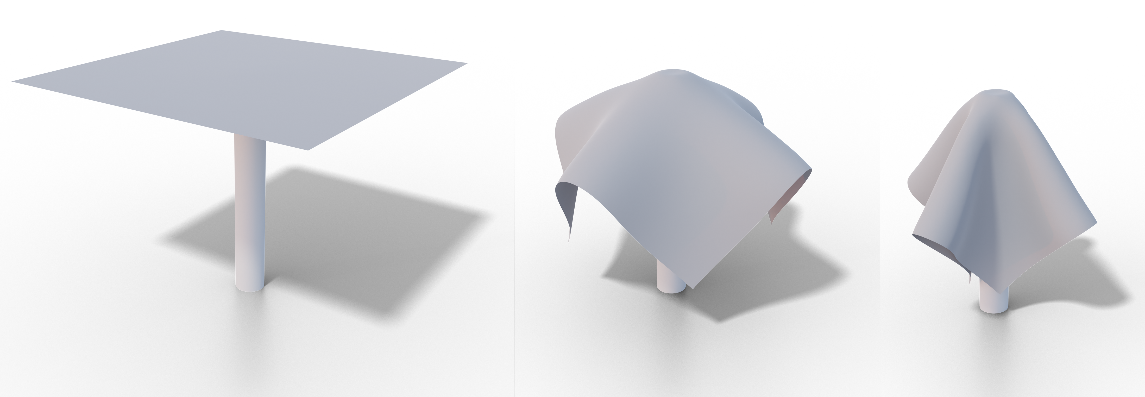
Figure 9. Several frames of a cloth simulation using the method of Baraff and Witkin (1998) as implemented by Wolff et al. (2021).

The classic cloth simulation method by Baraff and Witkin (1998) has been extended in several ways over the years and still enjoys popularity today. The method defines stretching, shearing, and bending energies that lead to damping and direct forces. The method is implicit and solves a linear system at each time step. However, the majority of the time is spent constructing the linear system, which poses a performance bottleneck. To demonstrate the practicality of our system for more complex computations, we generate code for assembling the system matrix and the right-hand side. To this end we run a templated version of an implementation provided by Wolff et al. (2021). The final system has the form

$$\mathbf{A}=\mathbf{M} -h(\mathbf{D}_{\mathrm{stretch}}+\mathbf{D}_{\mathrm{shear}}+\mathbf{D}_{\mathrm{bend}})$$

$$+h^{2}(\mathbf{K}_{\mathrm{stretch}}+\mathbf{K}_{\mathrm{shear}}+\mathbf{K}_{\mathrm{bend}})$$

where $\mathbf{M}$ is the mass matrix and $\mathbf{K}$ and $\mathbf{D}$ are stiffness and damping matrices, respectively. All matrices are constructed by combining dense per-element contributions and we tag these blocks for the stretch and shear energies explicitly (see Section 4.2.4). Computing the local Hessians of the stretch and shear energy takes 587ms for a mesh with 100k vertices using our reference implementation. Generating code without tagging improves runtime by a factor of 5 (104ms) while enabling the feature gives a factor of 40 (14.7ms) in speedup. All three measurements have been conducted on Intel using a single thread. In Figure 8 we compare the performance of our method with the original implementation. All timings are measured on our Intel machine and are reported relative to the time it takes to factor the system matrix (Pardiso, 8 threads, Intel MKL). With increasing mesh size, the relative time spent on factorization increases. In all cases, we can significantly improve the performance and remove the bottleneck of system construction. The GPU timings include data transfer from and to the device; thus, the system construction becomes a negligible part of the overall runtime.

5.6.1. Automatic differentiation of deformation energies

Figure 10. Our system offers two options to efficiently compute the Hessian and gradient of a deformation energy (Baraff and Witkin, 1998): We can either directly compile optimized code based on an existing implementation, or employ automatic differentiation based on a symbolic representation of the energy integrated over the mesh. Both versions are competitive and provide significant speedups over the original implementations (reference times in parenthesis). Timings taken on AMD.

Several parts of the system matrix and its right-hand side are constructed from gradients and Hessians of deformation energies. To demonstrate our symbolic auto differentiation feature, we focus on the sum of stretch and shear energies and compute their gradient and Hessian. This gives us two methods to generate code computing derivatives for a specific mesh: (1) We can directly generate derivative expressions based on the implemented energy using automatic differentiation or (2) we can use run the hand optimized code for constructing gradient and Hessian using our symbolic type just as in the previous experiment. In all cases, we achieve at least an order of magnitude performance increase. Interestingly, both versions are competitive with a slight benefit for direct compilation of hand-optimized code when using a single thread only. However, the differences in implementation complexity are huge since the energy formulation is typically quite simple compared to the gradient and Hessian.

5.7. Comparison to classic automatic differentiation

Figure 11. We compare to overloading based automatic differentiation (Jakob, 2010) and a direct code transformation strategy (Desai et al., 2020). All timings include the generation of Hessians and gradients per-face of a deformation energy for a mesh with 1M vertices. Due to our expression optimization techniques, we can outperform competing approaches even without enabling vectorization and parallelization. For the competing methods we run implementations provided by the authors of (Desai et al., 2020). CPU timings taken on Intel.

There exists a variety of automatic differentiation techniques. We compare here with implementations of the two most prevalent techniques, overloading based automatic differentiation (Jakob, 2010), also known as backpropagation, and direct source code transformation (Desai et al., 2020). We compare using a benchmark example provided by Desai et al. (2020) that computes local Hessians of the symmetric Dirichlet deformation energy (Figure 11). Our method outperforms both techniques. In contrast to Jakob (2010) we do not have to maintain data structures to keep track of derivatives at runtime. Storing intermediate results and optimization expressions also gives us an advantage over direct code transformation techniques such as Desai et al. (2020).

5.8. Comparison to linear algebra packages

Sparse matrix multiplication is supported by most linear algebra libraries and packages. We compare our method to competing methods on three platforms in Table 1. Highly optimized implementations of sparse matrix-matrix multiplication (spmm) can analyze a specific problem instance and try to find an optimal ordering and grouping of operations based on tiling strategies. These optimizations extensively use specific properties of matrix multiplication. Our method on the other hand is more general and is not aware of the fact that an spmm operation is computed. All methods that use problem specific optimizations in any form are marked with the $\dagger$ symbol (preprocessing is not included in the timings). All other methods use general purpose spmm methods. For MKL we include both variants: with preprocessing using the 2-stage matrix multiplication mkl_sparse_sp2m and without using mkl_sparse_spmm. Our method generates code that is faster than both versions. The taco compiler (Kjolstad et al., 2017) can generate optimized and parallelized code from very concise descriptions of sparse linear algebra operations. For the comparison we used a hand optimized schedule with explicit storage of intermediate results as suggested by the authors (Kjolstad et al., 2019). Taco significantly improves over Eigen’s and MKL’s performance. On Vega we are able to outperform AMD’s optimized sparse matrix algebra rocSparse (AMD, 2020). However, on GTX cuSPARSE (Nvidia, 2020) is about 50% faster than our method. Apart from the timings we note that our method shares the advantage of taco that optimized code is automatically generated for different variants of matrices and operation flavors (transposing factors, computing only specific elements etc.). MKL, rocSparse and cuSparse support only some of these variants using many parameters. Performing spmm with cuSparse, for example, requires three function calls with about 10 parameters each and the allocation and management of several buffers (Nvidia, 2020, 15.6.16).

5.9. Ablation study

		+	+	+	+	+	+	+	+
	reference (Intel)	group	explicit tagging	local decompose	global decompose	simplify	optimize memory	vectorize	parallelize (8 threads)	final speedup
Cloth Hessian, 20k vertices, float, values only
Intel	136ms	50ms	13ms	2.9ms	2.9ms	2.9ms	2.7ms	0.81ms	0.15ms	906x
Autodiff (Intel)	136ms	-	18ms	4.9ms	4.9ms	4.2ms	3.9ms	0.96ms	0.18ms	755x
Vega	136ms	28ms	0.16ms	0.16ms	0.16ms	0.15ms	0.04ms	-	-	3400x
Autodiff (Vega)	136ms	-	0.15ms	0.15ms	0.15ms	0.14ms	0.04ms	-	-	3400x
Cloth Hessian, 20k vertices, float, values and sparse matrix construction
Intel	200ms	50ms	18ms	7.5ms	7.5ms	7.5ms	7.1ms	5.8ms	1.4ms	142x
Autodiff (Intel)	200ms	-	24ms	10ms	10ms	9.0ms	8.8ms	6.4ms	1.4ms	142x
Vega	200ms	27ms	0.35ms	0.35ms	0.35ms	0.35ms	0.24ms	-	-	833x
Autodiff (Vega)	200ms	-	0.42ms	0.35ms	0.35ms	0.34ms	0.23ms	-	-	870x
Cotan Laplacian, 200k vertices, float
Intel	105ms	31ms	-	31ms	15ms	14ms	13ms	13ms	3.2ms	33x
Vega	105ms	1.62ms	-	1.53	0.57	0.56	0.48	-	-	219x
$\mathbf{L}^{3}$, sparse, $\mathbf{L}\in\mathds{R}^{50k\times 50k}$, float
Intel	145ms	29ms	-	28ms	12ms	12ms	12ms	11ms	4.3ms	34x
Vega	145ms	1484ms	-	1479ms	0.55ms	0.55ms	0.49ms	-	-	296x

Table 2. We performed an ablation study to assess the influence of our optimization steps. In each column we incrementally activate a new feature. We start with simple grouping, similar to EGGS (Tang et al., 2020b). Next we allow for manually tagging Section 4.2.4, local (per kernel) and global expression decomposition to precompute redundant subexpressions Section 4.2, expression simplification Section 4.5, memory optimizations as well as vectorization and parallelization Section 4.8. We report the overall speedup over the reference implementation measured on Intel. We report timings averaged over 100 iterations both for CPUs and a GPUs. For the computation of the stretch and shear energy from (Baraff and Witkin, 1998) we compare hand written code and code generated by symbolic automatic differentiation. For timings that show less than 5% performance improvement over the last optimization step we use the color gray. All experiments have been conducted on Intel with single precision. Speedups using double precision on AMD for the cotan and cloth Hessian example can be found in Figure 5 and Figure 10, respectively.

The performance gains achieved by our method are a result of the combination of several optimization steps (Section 4). We perform an ablation study to investigate how much effect the individual features have. To this end we activate them one by one until we arrive at the full method. The results are presented in Table 2. In all cases, the C++ compiler producing the final program is free to use all optimizations enabled with -O3 and auto vectorization. Consequently all performance improvements are due to our optimization steps. We show timings for the cloth example as well as for the construction of the cotan Laplacian and the computation of the third power of a sparse matrix. For the cloth energy Hessian we show two variants: using our method on hand optimized code and on expressions generated using symbolic automatic differentiation (Section 5.6.1). The experiments are conducted for the computation of the per-element Hessians with and without sparse matrix construction. The reason for showing these experiments individually is their different performance behavior. The per-element Hessian computation is highly parallel and compute intensive while matrix assembly requires many memory accesses to sum up entries of the local Hessians. In the following we elaborate on the effect individual optimization steps.

Grouping

The most basic approach is simple grouping. This means, we consider all output expressions as they are and sort them into structurally equivalent groups forming kernels. Unrolling these expressions already gives a considerable performance improvement; however, in many cases this produces an excessive amount of kernels that have a few instances only. For the last example, the computation of $\mathbf{L}^{3}$, basic grouping generates about 16 thousand kernels, most of them having one member only. The generated code files have a size of about 30 MB and need several hours to compile using clang. Since these kernels cannot easily be parallelized, they also do not profit from GPUs.

Explicit tagging

We use explicit tagging only for the cloth examples, where we introduce a single function call for tagging the per-element $9\times 9$ Hessian as intermediate (see Section 4.2.4). This ensures that they are all evaluated within one kernel making optimal use of local expression sharing. GPUs especially benefit from this step since the number of kernels and memory traffic are both greatly reduced.

Local decomposition

Using grouping with local decomposition roughly corresponds to the method implemented in EGGS (Tang et al., 2020b). Caching common subexpression per kernel is especially useful for compute bound programs running on the CPU. While C++ compilers implement similar techniques, they are not as powerful as our algebraic decomposition method as witnessed by the speedup generated by this step.

Global decomposition

Being able to compute subexpressions such that they can be reused by other kernels not only saves time but also allows for a smaller number kernels in many cases. For the computation of $\mathbf{L}^{3}$, for example, the number of kernels is only 21 instead of 16000 without decomposition. Automatic decomposition also enables the efficient use of GPUs int this case. We do not see a benefit for computing the Hessian because explicit tagging of local Hessians already decomposes the computation in a nearly optimal way. For all other examples we see more than a factor of two in performance difference.

Simplification

The effect of expression simplification shows only in compute-bound scenarios. It is especially helpful for expressions generated by symbolic automatic differentiation. Other examples are based on code that has been optimized by hand and therefore does not result in expressions with a lot of optimization potential.

Memory optimization

Optimizing memory access encompasses several optimizations described in Section 4.8. One of the most effective allows for coalesced memory access when writing intermediate values or loading position indices and constants. The GPU version of the first example benefits the most from this method. The optimizations are not as efficient for the full Hessian matrix construction because most memory accesses load intermediates that cannot be optimized. The reason is that the storage locations for intermediates have already been fixed by our system when writing their values.

Vectorization

We support vectorization by using nested loops and blocked coalesced memory access as described in Section 4.8. Again, compute-bound algorithms benefit the most from this feature. Note that auto-vectorization of the C++ compiler is activated for all tests but really makes a difference when used together with our vectorization-friendly code and memory optimizations.

Parallelization

Since all instances of a kernel can be evaluated independently, we can trivially employ parallelization and obtain considerable speedups. This also helps memory-bound application by using multiple memory controllers. The ablation study shows that the performance boosts due to different optimization steps vary depending on the device and type of algorithm. However, no optimization step decreases performance. Combining all stages makes for a versatile code optimization technique that tries to use features of the target device as efficiently as possible.

6. Limitations and Concluding Remarks

We introduced a compiler for algorithms with a static execution tree that shows that speedups of two to three orders of magnitude can be achieved by unrolling the computational tree, and then regrouping expressions in a hardware friendly way. Our reference implementation shows that this approach is very promising and practical. There are, however, a few engineering aspects that would require additional work to make this method more accessible. (1) The numerical types of the code need to be templates to be compatible with our symbolic type. Automatically replacing types for non-templated code would make our method even more practical. (2) The central limitation of our method is that it is time and memory expensive. Therefore it is useful if the code to be optimized is executed many times. For this paper our focus was on reducing the running time, however, code optimization time as well as memory consumption can likely be reduced by a significant factor by optimizing and parallelizing the pipeline and compressing expression trees. (3) The current compilation process is serial and not optimized. We believe that with more engineering the compilation time and memory requirements could be dramatically reduced. (4) Finally we would like to remove the need to automatically annotate dense blocks in order to evaluate several expressions in a single kernel. This could be achieved by searching all expression trees for potential dense blocks. We believe that the main avenue for future work, apart from the points listed below, is to extend our approach to target multiple processors and accelerators, while taking into account the latency in the channels connecting them. The idea is to add to the input a description of the system (for example, a pair of GPUs in the same machine connected via PCIExpress, or a collection of 10 workstations in a local ethernet network), and generate an optimal execution policy that distributes the data and computation across all the available resources by taking advantage of the knowledge of the entire computational graph. We believe this is an exciting direction that could dramatically lower the barrier for developing research code on heterogeneous HPC clusters using a combination of CPUs, GPUs, and TPUs.

6.1. Compiler pass vs. code generator

A key design decision for our tool was to build a code generator leveraging phased compilation, rather than integrating our methodology into an existing compiler infrastructure such as LLVM; for example, we could have used an approach similar to profile-guided optimization to first compile code with instrumentation that generates traces for a second compilation step. Integrating within LLVM would have some advantages, including implementations of several optimization techniques we utilize. Instead of generating C++ source code, such an approach could generate LLVM IR. Alternatively, we could have attempted a purely-static approach that, instead of utilizing a two-phase compilation approach, used the combination of input values and LLVM IR to interpret or otherwise symbolically determine expression trees based on the input values at compile-time. With this approach, we would need to either utilize LLVM’s own interpretation framework or write our own, along with infrastructure to read sparse values from input files. In either alternative design, much of the the framework would be similar to our code generator: we still would need to process expression trees or similar data structures, and perform expression grouping and leaf harvesting. Expression optimization could utilize existing pieces of the LLVM framework, but we would likely need to write our own passes as well. In addition, the alternate designs would require generating LLVM IR rather than strings. In the end, we rejected these alternatives due to the simple fact that they would require writing more code than for our approach. We leave integrating with LLVM or another compiler infrastructure, which could lead to additional speedups and wider applicability, to future work.

Appendix A Algebraic hashing

Name: algebraicHash(SymbolicExpression x)

Output: Algebraic hash value for expression x.

if hashIsValid then // return hash if it has been computed. return h else

if Op(x) == Variable then h = Hash(VariableIndex(x)) else if Op(x) == Constant then if isSmallInteger(Value(x)) then h = Value(x) else h = Hash(Value(x)) end if

else if Op(x) == Multiplication then h = 1

foreach c in Childs(x) do h *= algebraicHash(c) end foreach

else if Op(x) == Addition then h = 0

foreach c in Childs(x) do h += algebraicHash(c) end foreach

else foreach c in Childs(x) do h = Hash(algebraicHash(c), h) end foreach

end if

h = Hash(Hash(Op(x)), h)

return h end if

ALGORITHM 2 Algebraic Hashing

Algorithm 2 presents pseudo code for our algebraic hashing procedure descibed in Section 4.1.2. If two expressions have the same algebraic hash value, they will evaluate to the same value; however, there are equivalent expressions that can not be detected like $\sin(x+\pi/2)$ and $\cos(x)$.

Appendix B Leaf harvesting example

In the illustrated example (Figure 2), leaf harvesting would result in the following array of data which contains the specific variable or constant stored in the $6$ leaves of each group member.

	$l_{0}$	$l_{1}$	$l_{2}$	$l_{3}$	$l_{4}$	$l_{5}$
tree 1	b	b	2	a	3.1	a
tree 2	c	c	2	d	2.7	d
	$x_{0}$	$x_{0}$	2	$x_{1}$	$c_{0}$	$x_{1}$

$x_{0}$	$x_{1}$	$c_{0}$
b	a	3.1
c	d	2.7

From this data, we can see that leaves $l_{0}$, and $l_{1}$ always contain the same variable. The same is true for $l_{3}$ and $l_{5}$. Leaf $l_{3}$ always contains the uniform constant $2$ which can be hard-coded and leaf $l_{4}$ contains a varying constant that has to be read from memory. This analysis will reduce the use of memory bandwidth since we can avoid redundant loads or even avoid them completely (Section 4.6).

Appendix C Automatic differentiation

Name: differentiate(Symbolic x)

Output: Gradient of the expression x.

grad = (0, …, 0)

stack $\leftarrow$ (x, 1)

while not isEmpty(stack) do y = pop(stack)

switch op(y[0]) do case Add do stack $\leftarrow$ (left(y[0]), y[1])

stack $\leftarrow$ (right(y[0]), y[1]) end case

case Sub do stack $\leftarrow$ (left(y[0]), y[1])

stack $\leftarrow$ (right(y[0]), -y[1]) end case

case Mul do stack $\leftarrow$ (left(y[0]), y[1] * right(y[0]))

stack $\leftarrow$ (right(y[0]), y[1] * left(y[0])) end case

case Div do stack $\leftarrow$ (left(y[0]), y[1] / right(y[0]))

stack $\leftarrow$ (right(y[0]), -left(y[0]) / (right(y[0]) * right(y[0])) * y[1]) end case

case VAR do grad[varId(y[0])] += y[1] end case

end switch

end while

return grad

ALGORITHM 3 Differentiation of a symbolic expression.

In Algorithm 3 we outline a simple version of our reverse-mode differentiation implementation following the concise treatment of Baydin et al. (2018). The listing illustrates that it is quite simple to add symbolic differentiation capabilities based on our Symbolic type. Moreover, adding support for additional operations is trivial and amounts to adding a case statement that defines the derivative of an operation with respect to the operands. The algorithm traverses the derivatives from the expression tree root down to it’s leaves motivating the name reverse-mode differentiation. The functions left and right access the first and second child of an expression; the operator $\leftarrow$ pushes elements onto the stack.

figure	experiment	size	execute code	analyze expressions	generate	peak Mem.	compile (gcc)	binary
3	numeric_0	100k	1m 21s 458ms	2m 54s 911ms	1s 472ms	7.7GB	1s 149ms	36KB
3	numeric_1	100k	2m 3s 939ms	4m 35s 377ms	2s 435ms	11.7GB	1s 122ms	36KB
3	numeric_2	100k	1m 54s 64ms	3m 30s 903ms	1s 773ms	10.1GB	1s 88ms	36KB
3	numeric_0	500k	7m 41s 301ms	14m 55s 165ms	8s 564ms	38.7GB	1s 97ms	36KB
3	numeric_1	500k	11m 40s 599ms	22m 20s 401ms	11s 797ms	58.1GB	1s 58ms	36KB
3	numeric_2	500k	10m 56s 974ms	17m 14s 999ms	9s 547ms	50.7GB	1s 75ms	36KB
3	numeric_0	1M	15m 12s 281ms	30m 5s 612ms	17s 283ms	77.4GB	1s 43ms	36KB
3	numeric_1	1M	26m 5s 690ms	47m 6s 461ms	26s 563ms	116.2GB	1s 52ms	36KB
3	numeric_2	1M	21m 58s 634ms	34m 25s 969ms	20s 128ms	99.6GB	1s 49ms	36KB
5	cotan	1M	1m 39s 345ms	11m 27s 881ms	8s 300ms	40.9GB	1s 544ms	57KB
5	cotan	500k	48s 568ms	5m 24s 992ms	4s 131ms	19.9GB	1s 490ms	57KB
5	cotan	200k	20s 607ms	2m 17s 935ms	1s 930ms	8.2GB	1s 473ms	57KB
6	dual Laplace	100k	5m 1s 537ms	42m 14s 675ms	24s 175ms	136.0GB	7s 421ms	343KB
6	dual Laplace	20k	47s 852ms	7m 15s 740ms	4s 356ms	29.6GB	7s 473ms	327KB
6	dual Laplace	7k	16s 49ms	2m 23s 564ms	1s 415ms	10.0GB	7s 503ms	258KB
10	cloth Hessian AD	100k	19m 46s 671ms	6m 37s 590ms	83ms	122.9GB	1s 509ms	57KB
10	cloth Hessian AD	50k	9m 6s 206ms	2m 25s 926ms	37ms	56.6GB	1s 603ms	57KB
10	cloth Hessian AD	20k	4m 2s 526ms	51s 499ms	17ms	25.0GB	1s 516ms	57KB
10	cloth Hessian direct	100k	2m 44s 437ms	3m 5s 543ms	143ms	18.4GB	1s 515ms	61KB
10	cloth Hessian direct	50k	1m 31s 336ms	1m 12s 900ms	49ms	8.5GB	1s 397ms	58KB
10	cloth Hessian direct	20k	33s 512ms	24s 217ms	25ms	3.7GB	1s 587ms	58KB
11	symmetric Dirichlet	1M	7m 0s 371ms	8m 26s 669ms	556ms	135.2GB	1s 272ms	61KB
7	ARAP rhs	300k	5m 12s 580ms	6m 16s 664ms	506ms	34.3GB	3s 127ms	248KB
8	cloth full system	100k	4m 36s 584ms	6m 10s 303ms	6m 10s 303ms	37.0GB	4s 521ms	207KB
8	cloth full system	50k	2m 7s 959ms	3m 32s 458ms	3m 32s 458ms	17.0GB	4s 543ms	135KB
8	cloth full system	20k	55s 56ms	57s 404ms	57s 404ms	7.5GB	4s 521ms	131KB

Table 3. We break down system performance for different stages of our method as well as the use of resources for all our examples.

Appendix D Expression simplification

We implemented the following set of transformations, and we introduce each of them with a typical example.

Factorization

For every sum of products we find the largest set of factors that is contained in as many factors as possible. This enables the following algebraic transformation:

$$xyz+xwy+vxy+ux \rightarrow xy(z+w+v)+ux$$

$$\rightarrow x(y(z+w+v)+u).$$

The algorithm tries to factor out the largest expression $xy$ first even though it is not contained in all summands. Recursively calling the factorization routine allows us to further simplify the expression by factoring out $x$ as well.

Reducing fractions

We analyze each subtree that contains only multiplications and divisions. By first expanding it into a pure product we can perform the following type of simplification:

$$\frac{(x+y)z^{2}}{(x+y)^{2}w}\frac{w^{2}}{z} \rightarrow(x+y)z^{2}\frac{1}{(x+y)^{2}}\frac{1}{w}w^{2}\frac{1}{z}\rightarrow\frac{zw}{(x+y)}.$$

In this step, we also find reciprocals of square roots, which allows us to compute them using fast implementations like Cuda’s rsqrt if available.

Summand elimination

By analyzing all subtrees of additions in a similar way, we can perform the transformation

$$(x+x+y-2(y+x))\rightarrow 2x+y+(-2y)+(-2x)\rightarrow-y.$$

All products of constants with sums are expanded to group multiples of expressions. Negative sums are treated as the product of a sum with the constant $-1$.

Square root elimination

Square roots commonly appear when normalizing vectors or computing angles between them. We consolidate products and divisions of square roots in order to minimize computational effort. We can also eliminate square roots of squares that would appear in a naive implementation of the squared norm

$$\left\|\begin{pmatrix}x\\ y\end{pmatrix}\right\|^{2}=\sqrt{x^{2}+y^{2}}\sqrt{x^{2}+y^{2}}\rightarrow\sqrt{(x^{2}+y^{2})(x^{2}+y^{2})}\rightarrow x^{2}+y^{2}.$$

Constant expressions

Arithmetic hashing allows us to predict if a complex expression will evaluate to a constant value. This gives us a powerful tool to simplify expressions that cannot be explicitly transformed into a simpler version but still evaluate to a constant. The basic transformation

$$\frac{(x-y)^{2}+xy}{x^{2}-xy+y^{2}}\rightarrow 1$$

is only possible because the value hash of the expression evaluates to one.

Appendix E Data structures

Our implementation is build around the Symbolic type that is replacing floating point values. A basic, unoptimized definition of this type is presented in the following listing.

⬇

class Symbolic {

\parstruct SData {

int opCode;

vector<Symbolic> childs;

int variable_id;

double constant;

\parsize_t structureHash();

size_t algebraicHash();

unsigned complexity();

};

\parshared_ptr<SData> data;

\parpublic:

Symbolic(int opCode, vector<Symbolic>& operands);

Symbolic(double constant);

Symbolic(int variableType, int variableId);

Symbolic operator+(const Symbolic& b);

Symbolic operator+=(const Symbolic& b);

…

};

\parSymbolic operator+(const double f, Symbolic& b);

Symbolic operator+(Symbolic& b, const double f);

Symbolic operator+=(Symbolic& b, const double f);

Symbolic sqrt(Symbolic& s);

…

The Symbolic type itself only stores a shared pointer to the actual data which is implemented as a nested type. The class Symbolic is responsible for overloading the required arithmetic operators while library functions and arithmetic operations involving floating point values are overloaded externally. Using the shared pointers makes memory management convenient and allows to save on memory as trees representing a local variable are stored only once even though the variable might be involved in different operations.

Appendix F Code optimization timings

In Table 3 we show a breakdown of the time and resources our system needed in order to generate the final, optimized program for all examples shown in the paper. The timings do not depend on the target architecture. The execution phase runs the original program with symbolic types. The analysis includes expression decomposition and grouping, leaf harvesting, and expression optimization. Code generation writes the code file and constructs all position indices for indirect memory access. Compilation creates the final program based on the generated code (we use gcc in this case). Most time is spent analyzing the expressions and their dependencies since all subexpressions above the complexity threshold have to be considered, indexed, and eventually decomposed. Compilation times and the final binary size are largely independent of the problem size which is expected since the expression will decompose into very similar sets of groups; they will just contain more instances. A crucial limitation of our method is the high memory demand for storing all expression trees, however, we show examples with up to a million vertices which is, depending on the context, relatively large. Our code is in large parts not optimized and would benefit from parallelization and advanced memory optimization.

References

- (1)
- Aho et al. (2013) AV Aho, Monica S Lam, R Sethi, and JD Ullman. 2013. Compilers: Pearson New International Edition: Principles, Techniques, and Tools. Pearson.
- Alexa et al. (2020) Marc Alexa, Philipp Herholz, Maximilian Kohlbrenner, and Olga Sorkine-Hornung. 2020. Properties of Laplace Operators for Tetrahedral Meshes. Computer Graphics Forum (proceedings of SGP 2020) 39, 5 (2020), 12 pages. https://doi.org/10.1111/cgf.14068
- AMD (2020) AMD. 2020. rocmSPARSE. https://rocsparse.readthedocs.io/en/master/
- Anderson et al. (1999) E. Anderson, Z. Bai, C. Bischof, S. Blackford, J. Demmel, J. Dongarra, J. Du Croz, A. Greenbaum, S. Hammarling, A. McKenney, and D. Sorensen. 1999. LAPACK Users’ Guide (third ed.). Society for Industrial and Applied Mathematics, Philadelphia, PA.
- Augustine et al. (2019) Travis Augustine, Janarthanan Sarma, Louis-Noël Pouchet, and Gabriel Rodríguez. 2019. Generating Piecewise-Regular Code from Irregular Structures. In Proceedings of the 40th ACM SIGPLAN Conference on Programming Language Design and Implementation (Phoenix, AZ, USA) (PLDI 2019). Association for Computing Machinery, New York, NY, USA, 625–639. https://doi.org/10.1145/3314221.3314615
- Balay et al. (1997) Satish Balay, William D Gropp, Lois Curfman McInnes, and Barry F Smith. 1997. Efficient management of parallelism in object-oriented numerical software libraries. In Modern software tools for scientific computing. Springer, Birkhäuser Boston, 163–202.
- Baraff and Witkin (1998) David Baraff and Andrew Witkin. 1998. Large Steps in Cloth Simulation. In Proceedings of the 25th Annual Conference on Computer Graphics and Interactive Techniques (SIGGRAPH ’98). Association for Computing Machinery, New York, NY, USA, 43–54. https://doi.org/10.1145/280814.280821
- Baydin et al. (2018) Atilim Gunes Baydin, Barak A Pearlmutter, Alexey Andreyevich Radul, and Jeffrey Mark Siskind. 2018. Automatic differentiation in machine learning: a survey. Journal of machine learning research 18 (2018).
- Bernstein et al. (2016) Gilbert Louis Bernstein, Chinmayee Shah, Crystal Lemire, Zachary Devito, Matthew Fisher, Philip Levis, and Pat Hanrahan. 2016. Ebb: A DSL for Physical Simulation on CPUs and GPUs. 35, 2, Article 21 (may 2016), 12 pages. https://doi.org/10.1145/2892632
- Bezanson et al. (2012) Jeff Bezanson, Stefan Karpinski, Viral B. Shah, and Alan Edelman. 2012. Julia: A Fast Dynamic Language for Technical Computing.
- Bik and Wijshoff (1993) Aart JC Bik and Harry AG Wijshoff. 1993. Compilation techniques for sparse matrix computations. In Proceedings of the 7th international conference on Supercomputing. ACM, 416–424.
- Bik and Wijshoff (1994) Aart JC Bik and Harry AG Wijshoff. 1994. On automatic data structure selection and code generation for sparse computations. In Languages and Compilers for Parallel Computing. Springer, 57–75.
- Bollhöfer et al. (2020) Matthias Bollhöfer, Olaf Schenk, Radim Janalik, Steve Hamm, and Kiran Gullapalli. 2020. State-of-the-Art Sparse Direct Solvers. (2020), 3–33. https://doi.org/10.1007/978-3-030-43736-7_1
- Byun et al. (2012) Jong-Ho Byun, Richard Lin, Katherine A Yelick, and James Demmel. 2012. Autotuning sparse matrix-vector multiplication for multicore. EECS, UC Berkeley, Tech. Rep (2012).
- Cheshmi et al. (2018) Kazem Cheshmi, Shoaib Kamil, Michelle Mills Strout, and Maryam Mehri Dehnavi. 2018. ParSy: Inspection and Transformation of Sparse Matrix Computations for Parallelism. In Proceedings of the International Conference for High Performance Computing, Networking, Storage, and Analysis (Dallas, Texas) (SC ’18). IEEE Press, Piscataway, NJ, USA, Article 62, 15 pages. http://dl.acm.org/citation.cfm?id=3291656.3291739
- Chou et al. (2018) Stephen Chou, Fredrik Kjolstad, and Saman Amarasinghe. 2018. Format Abstraction for Sparse Tensor Algebra Compilers. Proc. ACM Program. Lang. 2, OOPSLA, Article 123 (Oct. 2018), 30 pages. https://doi.org/10.1145/3276493
- Desai et al. (2020) Deshana Desai, Etai Shuchatowitz, Zhongshi Jiang, Teseo Schneider, and Daniele Panozzo. 2020. ACORNS: An Easy-To-Use Code Generator for Gradients and Hessians. arXiv:2007.05094 [cs.MS]
- Devito et al. (2017) Zachary Devito, Michael Mara, Michael Zollhöfer, Gilbert Bernstein, Jonathan Ragan-Kelley, Christian Theobalt, Pat Hanrahan, Matthew Fisher, and Matthias Niessner. 2017. Opt: A Domain Specific Language for Non-Linear Least Squares Optimization in Graphics and Imaging. ACM Trans. Graph. 36, 5, Article 171 (oct 2017), 27 pages. https://doi.org/10.1145/3132188
- Feautrier (1988) Paul Feautrier. 1988. Array Expansion. In 2nd International Conference on Supercomputing (ICS’88). ACM, 429–441.
- Google (2017) Google. 2017. TensorFlow Sparse Tensors. https://www.tensorflow.org/api_guides/python/sparse_ops.
- Goto and van de Geijn (2008) Kazushige Goto and Robert A. van de Geijn. 2008. Anatomy of High-Performance Matrix Multiplication. ACM Trans. Math. Softw. 34, 3, Article 12 (May 2008), 25 pages.
- Griewank and Walther (2008) Andreas Griewank and Andrea Walther. 2008. Evaluating derivatives: principles and techniques of algorithmic differentiation. Vol. 105. Siam.
- Guennebaud et al. (2010) Gaël Guennebaud, Benoît Jacob, et al. 2010. Eigen v3. http://eigen.tuxfamily.org.
- Iglberger et al. (2012) Klaus Iglberger, Georg Hager, Jan Treibig, and Ulrich Rüde. 2012. High performance smart expression template math libraries. In 2012 International Conference on High Performance Computing Simulation (HPCS). 367–373. https://doi.org/10.1109/HPCSim.2012.6266939
- Intel (2021) Intel. 2021. Developer reference for Intel oneAPI Math Kernel Library - C. Technical Report. https://software.intel.com/content/dam/develop/external/us/en/documents/onemkl-developerreference-c.pdf.
- Jakob (2010) Wenzel Jakob. 2010. Mitsuba renderer. http://www.mitsuba-renderer.org.
- Kjolstad et al. (2019) Fredrik Kjolstad, Peter Ahrens, Shoaib Kamil, and Saman Amarasinghe. 2019. Tensor Algebra Compilation with Workspaces. (2019), 180–192. http://dl.acm.org/citation.cfm?id=3314872.3314894
- Kjolstad et al. (2017) Fredrik Kjolstad, Shoaib Kamil, Stephen Chou, David Lugato, and Saman Amarasinghe. 2017. The Tensor Algebra Compiler. Proc. ACM Program. Lang. 1, OOPSLA, Article 77 (Oct. 2017), 29 pages. https://doi.org/10.1145/3133901
- Kjolstad et al. (2016) Fredrik Kjolstad, Shoaib Kamil, Jonathan Ragan-Kelley, David Levin, Shinjiro Sueda, Desai Chen, Etienne Vouga, Danny Kaufman, Gurtej Kanwar, Wojciech Matusik, and Saman Amarasinghe. 2016. Simit: A Language for Physical Simulation. ACM Trans. Graphics (2016).
- Kotlyar et al. (1997) Vladimir Kotlyar, Keshav Pingali, and Paul Stodghill. 1997. A relational approach to the compilation of sparse matrix programs. In Euro-Par’97 Parallel Processing. Springer, 318–327.
- Liu et al. (2015) Baoyuan Liu, Min Wang, Hassan Foroosh, Marshall Tappen, and Marianna Pensky. 2015. Sparse Convolutional Neural Networks. In Proceedings of the IEEE Conference on Computer Vision and Pattern Recognition (CVPR).
- Mahmoud et al. (2021) Ahmed H. Mahmoud, Serban D. Porumbescu, and John D. Owens. 2021. RXMesh: A GPU Mesh Data Structure. ACM Transactions on Graphics 40, 4 (Aug. 2021). https://doi.org/10.1145/3450626.3459748
- Mara et al. (2021) Michael Mara, Felix Heide, Michael Zollhöfer, Matthias Nießner, and Pat Hanrahan. 2021. Thallo – Scheduling for High-Performance Large-Scale Non-Linear Least-Squares Solvers. ACM Trans. Graph. 40, 5, Article 184 (sep 2021), 14 pages. https://doi.org/10.1145/3453986
- MATLAB (2014) MATLAB. 2014. version 8.3.0 (R2014a). The MathWorks Inc., Natick, Massachusetts.
- McAdams et al. (2011) Aleka McAdams, Andrew Selle, Rasmus Tamstorf, Joseph Teran, and Eftychios Sifakis. 2011. Computing the singular value decomposition of 3x3 matrices with minimal branching and elementary floating point operations. Technical Report. University of Wisconsin-Madison Department of Computer Sciences.
- Nvidia (2020) Nvidia. 2020. cuSPARSE Library. Technical Report. https://docs.nvidia.com/cuda/pdf/CUSPARSE_Library.pdf.
- Pugh (1991) William Pugh. 1991. Uniform Techniques for Loop Optimization. In 5th International Conference on Supercomputing (ICS’91). ACM, 341–352.
- Ragan-Kelley et al. (2012) Jonathan Ragan-Kelley, Andrew Adams, Sylvain Paris, Marc Levoy, Saman Amarasinghe, and Frédo Durand. 2012. Decoupling Algorithms from Schedules for Easy Optimization of Image Processing Pipelines. ACM Trans. Graph. 31, 4, Article 32 (July 2012), 12 pages. https://doi.org/10.1145/2185520.2185528
- Ragan-Kelley et al. (2013) Jonathan Ragan-Kelley, Connelly Barnes, Andrew Adams, Sylvain Paris, Frédo Durand, and Saman Amarasinghe. 2013. Halide: A Language and Compiler for Optimizing Parallelism, Locality, and Recomputation in Image Processing Pipelines. In Proceedings of the 34th ACM SIGPLAN Conference on Programming Language Design and Implementation (Seattle, Washington, USA) (PLDI ’13). Association for Computing Machinery, New York, NY, USA, 519–530. https://doi.org/10.1145/2491956.2462176
- Sanderson (2010) Conrad Sanderson. 2010. Armadillo: An Open Source C++ Linear Algebra Library for Fast Prototyping and Computationally Intensive Experiments. Technical Report. NICTA.
- Senanayake et al. (2020) Ryan Senanayake, Changwan Hong, Ziheng Wang, Amalee Wilson, Stephen Chou, Shoaib Kamil, Saman Amarasinghe, and Fredrik Kjolstad. 2020. A Sparse Iteration Space Transformation Framework for Sparse Tensor Algebra. Proc. ACM Program. Lang. 4, OOPSLA, Article 158 (Nov. 2020), 30 pages. https://doi.org/10.1145/3428226
- Sorkine and Alexa (2007) Olga Sorkine and Marc Alexa. 2007. As-Rigid-As-Possible Surface Modeling. In Proceedings of EUROGRAPHICS/ACM SIGGRAPH Symposium on Geometry Processing. 109–116.
- Tang et al. (2020a) Haotian* Tang, Zhijian* Liu, Shengyu Zhao, Yujun Lin, Ji Lin, Hanrui Wang, and Song Han. 2020a. Searching Efficient 3D Architectures with Sparse Point-Voxel Convolution. In European Conference on Computer Vision.
- Tang et al. (2020b) Xuan Tang, Teseo Schneider, Shoaib Kamil, Aurojit Panda, Jinyang Li, and Daniele Panozzo. 2020b. EGGS: Sparsity-Specific Code Generation. Computer Graphics Forum 39, 5 (2020), 209–219. https://doi.org/10.1111/cgf.14080 arXiv:https://onlinelibrary.wiley.com/doi/pdf/10.1111/cgf.14080
- Van Der Walt et al. (2011) Stefan Van Der Walt, S Chris Colbert, and Gael Varoquaux. 2011. The NumPy array: a structure for efficient numerical computation. Computing in Science & Engineering 13, 2 (2011), 22–30.
- Van Zee and van de Geijn (2015) Field G. Van Zee and Robert A. van de Geijn. 2015. BLIS: A Framework for Rapidly Instantiating BLAS Functionality. ACM Trans. Math. Software 41, 3 (June 2015), 14:1–14:33. http://doi.acm.org/10.1145/2764454
- Venkat et al. (2015) Anand Venkat, Mary Hall, and Michelle Strout. 2015. Loop and Data Transformations for Sparse Matrix Code. In Proceedings of the 36th ACM SIGPLAN Conference on Programming Language Design and Implementation (Portland, OR, USA) (PLDI 2015). 521–532.
- Venkat et al. (2016) Anand Venkat, Mahdi Soltan Mohammadi, Hongbo Rong, Rajkishore Barik, Jongsoo Park, Michelle Mills Strout, and Mary Hall. 2016. Automating Wavefront Parallelization for Sparse Matrix Computations. In In Supercomputing (SC).
- Virtanen et al. (2020) Pauli Virtanen, Ralf Gommers, Travis E. Oliphant, Matt Haberland, Tyler Reddy, David Cournapeau, Evgeni Burovski, Pearu Peterson, Warren Weckesser, Jonathan Bright, Stéfan J. van der Walt, Matthew Brett, Joshua Wilson, K. Jarrod Millman, Nikolay Mayorov, Andrew R. J. Nelson, Eric Jones, Robert Kern, Eric Larson, C J Carey, İlhan Polat, Yu Feng, Eric W. Moore, Jake VanderPlas, Denis Laxalde, Josef Perktold, Robert Cimrman, Ian Henriksen, E. A. Quintero, Charles R. Harris, Anne M. Archibald, Antônio H. Ribeiro, Fabian Pedregosa, Paul van Mulbregt, and SciPy 1.0 Contributors. 2020. SciPy 1.0: Fundamental Algorithms for Scientific Computing in Python. Nature Methods 17 (2020), 261–272. https://doi.org/10.1038/s41592-019-0686-2
- Vuduc et al. (2005) Richard Vuduc, James W. Demmel, and Katherine A. Yelick. 2005. OSKI: A library of automatically tuned sparse matrix kernels. Journal of Physics: Conference Series 16, 1 (2005), 521+.
- Walter and Koch (2007) Joerg Walter and Mathias Koch. 2007. uBLAS. http://www.boost.org/libs/numeric/ublas/doc/index.htm
- Whaley and Dongarra (1998) R. Clint Whaley and Jack Dongarra. 1998. Automatically Tuned Linear Algebra Software. In SuperComputing 1998: High Performance Networking and Computing.
- Wolff et al. (2021) Katja Wolff, Philipp Herholz, Verena Ziegler, Frauke Link, Nico Brügel, and Olga Sorkine-Hornung. 2021. 3D Custom Fit Garment Design with Body Movement. arXiv:2102.05462 [cs.GR]