Cubature Method for Stochastic Volterra Integral Equations

Abstract

In this paper, we introduce the cubature formula for Stochastic Volterra Integral Equations. We first derive the stochastic Taylor expansion in this setting, by utilizing a functional Itô formula, and provide its tail estimates. We then introduce the cubature measure for such equations, and construct it explicitly in some special cases, including a long memory stochastic volatility model. We shall provide the error estimate rigorously. Our numerical examples show that the cubature method is much more efficient than the Euler scheme, provided certain conditions are satisfied.

MSC2020. 60H20, 65C30, 91G60

Keywords. Stochastic Volterra integral equations, cubature formula, stochastic Taylor expansion, fractional stochastic volatility model, rough volatility model

1 Introduction

Consider a stock price in a Brownian setting under risk neutral measure $\mathbb{P}$:

$$dS_{t}=S_{t}\sigma_{t}dB_{t},$$ (1.1)

In the Black-Scholes model, the volatility process $\sigma_{t}\equiv\sigma_{0}$ is a constant. There is a large literature on stochastic volatility models where $\sigma$ is also a diffusion process, see e.g. Fouque-Papanicolaou-Sircar-Solna [19]. Strongly supported by empirical studies, the fractional stochastic volatility models and rough volatility models have received very strong attention in recent years, where $\sigma$ satisfies the following Stochastic Volterra Integral Equation (SVIE):

$$\sigma_{t}=\sigma_{0}+\int_{0}^{t}K(t,r)V_{0}(\sigma_{r})dr+\int_{0}^{t}K(t,r)V_{1}(\sigma_{r})d\tilde{B}_{r}.$$ (1.2)

Here $\tilde{B}$ is another Brownian motion possibly correlated with $B$, $V_{i}$’s are appropriate deterministic functions, and the deterministic two time variable function $K$ has a Hurst parameter $H>0$ in the sense that $K(t,r)\sim(t-r)^{H-{1\over 2}}$ and $\partial_{t}K(t,r)\sim(t-r)^{H-{3\over 2}}$ when $t-r>0$ is small. Such a model was first proposed by Comte-Renault [10] for $H>{1\over 2}$, to model the long memory property of the volatility process. Another notable work is Gatheral-Jaisson-Rosenbaum [23], which finds market evidence that volatility’s high-frequency behavior could be modeled as a rough path with $H<{1\over 2}$. We remark that one special case of (1.2) is the fractional Brownian motion, where $V_{0}\equiv 0$ and $V_{1}\equiv 1$, see, e.g. Nualart [44].

Our goal of this paper is to understand and more importantly to numerically compute the option price in this market: assuming zero interest rate for simplicity,

$$\mathbb{E}[G(S_{T})].$$ (1.3)

Note that the volatility process $\sigma$ in (1.2) is in general neither a Markov process nor a semimartingale. Consequently, $S_{t}$ is highly non-Markovian, in the sense that one cannot Markovianize it by adding finitely many extra states, and correspondingly the option price is characterized as a path dependent PDE (PPDE, for short), see Viens-Zhang [51]. This imposes significant challenges, both theoretically and numerically. Indeed, compared to the huge literature on numerical methods for PDEs, there are very few works on efficient numerical methods for such PPDEs. Besides the standard Euler scheme Zhang [55], we refer to Wen-Zhang [53] for an improved rectangular method; Jacquier-Oumgari [31] and Ruan-Zhang [50] on numerical methods for high dimensional (nonlinear) PPDEs driven by SVIEs; Richard-Tan-Yang [48, 49] on discrete-time simulation schemes, including the Euler and Milstein schemes, and the corresponding Multi-Level Monte-Carlo method; Ma-Yang-Cui [41] by using Markov chain approximation; and Alfonsi-Kebaier [1], Bayer-Breneis [3], and Harms [29] by using Laplace transform for singular kernel functions. In recent years, there has also been a growing interest on the convergence analysis and error estimates for stochastic Volterra integral equations, see, e.g. Bayer-Fukasawa-Nakahara [4], Bayer-Hall-Tempone [5], Bonesini-Jacquier-Pannier [8], Friz-Salkeld-Wagenhofer [20], Fukasawa-Ugai [21], Gassiat [22], Li-Huang-Hu [35], and Nualart-Saikia [45]. In this paper, we propose the cubature method for the above option price (1.3). This is a deterministic method, and our numerical examples show that, under certain conditions, it is much more efficient than the simulation methods such as the Euler scheme.

The cubature method was first introduced by the seminal works Lyons-Victoir [40] and Litterer-Lyons [37] for diffusion processes, see also Gyurkó-Lyons [26], Litterer-Lyons [38], Ninomiya-Shinozaki [42], and Ninomiya-Victoir [43] for its extensive numerical implementations. The method builds upon the stochastic Taylor expansion for smooth $G$:

$$G(S_{T})=I_{N}+R_{N},$$ (1.4)

see, e.g. Kloeden-Platen [34], where $I_{N}$ is a linear combination of multiple integrals against the Brownian motion $B$ (typically in Stratonovich form), called the signatures of $B$, and $R_{N}$ is the remainder term. The main idea is to introduce a discrete measure $Q$ to match the expectations of the signatures: recalling that $\mathbb{E}=\mathbb{E}^{\mathbb{P}}$ is the expectation under $\mathbb{P}$,

$$\mathbb{E}[I_{N}]=\mathbb{E}^{Q}[I_{N}],$$ (1.5)

Then we will have an approximation $\mathbb{E}[G(S_{T})]\approx\mathbb{E}^{Q}[G(S_{T})]$. Since $Q$ is discrete and it is easy to compute the exact value of $\mathbb{E}^{Q}[G(S_{T})]$ (without involving simulations), the algorithm is very efficient, provided sufficient technical conditions to make the approximation error small enough.

In this paper we shall consider the general SVIE, see (2.1) below, and our goal is to approximate $\mathbb{E}[G(X_{T})]$. To introduce the cubature method for $X$, our first step is to derive the stochastic Taylor expansion in this setting. Note that (1.4) relies heavily on the Itô formula, but the solution $X$ to the SVIE is not a semimartinagle, which prohibits us from applying the Itô formula directly. To overcome this difficulty, we utilize an auxiliary two time variable process $\Theta^{s}_{t}$ introduced by Wang [52] and Viens-Zhang [51], see (2.6) below. This process satisfies $\Theta^{t}_{t}=X_{t}$ and enjoys the desired semimartingale property: for fixed $s$, the process $t\in[0,s]\mapsto\Theta^{s}_{t}$ is a semimartingale. In particular, [51] established a functional Itô formula, which enables us to derive the desired stochastic Taylor expansion, with more involved signatures for the SVIEs than the diffusion case. We then introduce a discrete cubature measure $Q$ for $X$, in the pirit of (1.4) and (1.5), and prove the following error estimate: for some constant $C_{N}$ which depends on the regularity of the coefficients,

$$\Big{|}\mathbb{E}[G(X_{T})]-\mathbb{E}^{Q}[G(X_{T})]\Big{|}\leq C_{N}T^{N+1\over 2}.$$ (1.6)

The above result is desirable only when $T$ is small. For general $T$, we follow the idea of [40, Theorem 3.3] and utilize the flow property of the path dependent value function established in [51]. To be precise, we consider a uniform partition of $[0,T]$: $0=T_{0}<\cdots<T_{M}=T$, and construct a cubature measure $Q_{m}$ on each subinterval $[T_{m},T_{m+1}]$. Let $Q$ be the independent composition of $\{Q_{m}\}_{0\leq m<M}$, we then have the following estimate:

$$\Big{|}\mathbb{E}[G(X_{T})]-\mathbb{E}^{Q}[G(X_{T})]\Big{|}\leq C_{N}{T^{N+1\over 2}\over M^{N-1\over 2}},$$ (1.7)

where $C_{N}$ is independent of $M$. The above estimate clearly converges to $0$ as $M\to\infty$.

We remark that, while our stochastic Taylor expansion can be developed for any kernel $K$ with Hurst parameter $H>0$, the cubature formula becomes much more subtle when $H<{1\over 2}$. In this paper we restrict to the case $H\geq{1\over 2}$, and leave the case $H<{1\over 2}$ to future study. For applications, we refer to Comte-Renault [10] for the long memory model with ${1\over 2}<H<1$, Gulisashvili-Viens-Zhang [24] for the integrated variance model with $1<H<2$, and El Omari [15] for the mixed fractional Brownian motion model with more general $H$. We also refer to Beran [6, Section 4.2] for applications in hydrology, Loussot-Harba-Jacquet-Benhamou-Lespesailles-Julien [39] for applications in image processing, Gupta-Singh-Karlekar [25] for applications in signal classification, Blu-Unser [7] for fractional spline estimators, and Perrin-Harba-Berzin Joseph-Iribarren-Bonami [47] for the theory of higher order fractional Brownian motions with general $H>1$. However, we should point out that our result does not cover the rough volatility models in Gatheral-Jaisson-Rosenbaum [23] with $0<H<{1\over 2}$. Moreover, the estimates (1.6) and (1.7) require the coefficients to be sufficiently smooth, as we will specify in the paper. In particular, the constant $C_{N}$ will depend on such regularity.

The efficiency of our cubature method comes down to the construction of the cubature measure $Q$ in (1.7), which will involve $(2W)^{M}$ deterministic paths for some constant $W$. When the dimension of $X$ is large, or when $N$ is large, the $W$ will be large; and when $T$ is large, in light of (1.7) we will require $M$ to be large. We refer to §7.5 for more precise comments on the efficiency issue. When all the conditions are satisfied so that $(2W)^{M}$ is at a reasonable level, our numerical examples show that the cubature method is much more efficient than the Euler scheme.

We should remark that the above efficiency issue was already present for the cubature method in the standard Brownian setting. There have been great efforts in the literature to overcome this difficulty and to apply the idea of the cubature method to more general models, see, e.g., Crisan-Manolarakis [11, 12], Crisan-McMurray [13], Raynal-Trillos [14], Filipović-Larsson-Pulido [16], Foster-Lyons-Oberhauser [17], Foster-Reis-Strange [18], and Hayakawa-Oberhauser-Lyons [30]. It will be very interesting to explore if these ideas can help to improve the cubature method in the Volterra framework. We would also like to mention the very interesting connection between the signature, the kernel method, and machine learning, see Chevyrev-Oberhauser [9], Kidger-Bonnier-Arribas-Salvi-Lyons [32], Kiraly-Oberhauser [33], Liao-Lyons-Yang-Ni [36], and the references therein.

Finally, we note that, while sharing many properties, the SVIE (1.2) is different from the following SDE driven by a fractional Brownian motion $B^{H}_{t}:=\int_{0}^{t}K(t,r)dr+\int_{0}^{t}K(t,r)d\tilde{B}_{r}$:

$$\sigma^{\prime}_{t}=\sigma_{0}+\int_{0}^{t}V_{0}(\sigma^{\prime}_{r})dr+\int_{0}^{t}V_{1}(\sigma^{\prime}_{r})dB^{H}_{r}.$$ (1.8)

We refer to Baudoin-Coutin [2] and Passeggeri [46] for some works on signatures for fractional Brownian motions, and Harang-Tindel [27, 28] on signatures defined for “ Volterra path”. We shall remark that, unlike our signature which is directly for the solution $\sigma_{t}$ to the SVIE (1.2) (instead of for the driving Brownian motion $\tilde{B}$), these signatures are for the driving fractional Brownian motion $B^{H}$ or “Volterra path” which has much simpler structure. In particular, their signatures do not lead to the desired stochastic Taylor expansion which is crucial for the cubature method.

The rest of the paper is organized as follows. In §2 we derive the stochastic Taylor expansions for the general SVIEs and prove the tail estimate. In §3 we introduce the cubature formula when $T$ is small, and in §4 we modify the cubature formula when $[0,T]$ is decomposed into $M$ parts. We construct the cubature measure $Q$ explicitly for a one dimensional SVIE in §5 , and for the $2$-dimensional fractional stochastic volatility model in §6. In §7 we present various numerical examples and compare its efficiency with the Euler scheme. Finally, we present some technical proofs in Appendix.

2 Stochastic Taylor expansions

Throughout this paper, let $(\Omega,{\cal F},\mathbb{F},\mathbb{P})$ be a filtered probability space, $B^{0}_{t}:=t$, and $B=(B^{1},\cdots,B^{d})$ a $d$-dimensional Brownian motion. Let $T>0$ be a fixed terminal time. We consider $d_{1}$-dimensional state process $X=(X^{1},\cdots,X^{d_{1}})$ solving the following SVIE under Stratonovich integration $\circ$ : given $x=(x_{1},\cdots,x_{d_{1}})\in\mathbb{R}^{d_{1}}$,

$$X^{i}_{t}=x_{i}+\sum_{j=0}^{d}\int_{0}^{t}K_{i}(t,r)V^{i}_{j}(X_{r})\circ dB^{j}_{r},\quad i=1,\cdots,d_{1},$$ (2.1)

and we are interested in the efficient numerical computation of

$$Y_{0}:=\mathbb{E}\big{[}G(X_{T})\big{]}.$$ (2.2)

Throughout the paper, the following hypotheses will always be enforced: for some $N\geq 1$ which will be specified in contexts,

(H0) Each $K_{i}:\{(t,r):0\leq r\leq t\leq T\}\to[0,\infty)$ is infinitely smooth on $\{r<t\}$, and either $K_{i}\equiv 1$ or $K_{i}$ has Hurst parameter $H_{i}>{1\over 2}$, that is, $K_{i}(t,r)\sim(t-r)^{H_{i}-{1\over 2}}$ and $\partial_{t}K_{i}(t,r)\sim(t-r)^{H_{i}-{3\over 2}}$ when $t-r>0$ is small.

(HN) The functions $V^{i}_{j},G\in C^{N}(\mathbb{R}^{d_{1}};\mathbb{R})$ with all the derivatives up to the order $N$ bounded.

For later purpose, we will also need the following stronger version of (H0).

(H0-N) Each $K_{i}:\{(t,r):0\leq r\leq t\leq T\}\to[0,\infty)$ is infinitely smooth on $\{r<t\}$, and either $K_{i}\equiv 1$ or $K_{i}$ has Hurst parameter $H_{i}>N+{1\over 2}$, in the sense that ${\partial^{\alpha+\beta}\over\partial t^{\alpha}\partial r^{\beta}}K_{i}(t,r)\sim(t-r)^{H_{i}-\alpha-\beta-{1\over 2}}$ when $t-r>0$ is small, for all integers $\alpha,\beta\geq 0$ such that $\alpha+\beta\leq N$.

Remark 2.1.

(i) When $K_{i}$ has Hurst parameter $H_{i}>{1\over 2}$, $X^{i}$ is Hölder-$(H_{i}\wedge 1-\varepsilon)$ continuous in $t$ for any small $\varepsilon>0$. This implies that $V(X^{i}_{t})\circ dB^{j}_{t}=V(X^{i}_{t})dB^{j}_{t}$ for any smooth function $V$, where $V(X^{i}_{t})dB^{j}_{t}$ denotes the Itô integral, and they coincide with the Young’s pathwise integral. On the other hand, when $K_{i}\equiv 1$, $X^{i}$ is clearly a semimartingale. So, letting $I_{0}$ denote the set of $i>0$ such that $K_{i}\equiv 1$, we may rewrite (2.1) in Itô’s form, and in particular they are wellposeded under (H0) and (H2):

$$X^{i}_{t}=x_{i}+\sum_{j=0}^{d}\int_{0}^{t}K_{i}(t,r)V^{i}_{j}(X_{r})dB^{j}_{r}+{1\over 2}\sum_{k\in I_{0}}\int_{0}^{t}K_{i}(t,r)\partial_{k}V^{i}_{j}(X_{r})V^{k}_{j}(X_{r})dr.$$ (2.3)

(ii) Consider a special case: $x_{1}=0$, $K_{1}\equiv 1$, $V^{1}_{0}\equiv 1$, $V^{1}_{j}\equiv 0$ for $j\geq 2$. Then we can easily see that $X^{1}_{t}=t$. So the system (2.1) actually covers the case that the coefficients $V^{i}_{j}$ depends on the time variable $t$.  

Remark 2.2.

(i) In fractional stochastic volatility models, where $X^{i}$ is interpreted as the volatility (or variance) process of certain underlying asset price, the assumption ${1\over 2}<H_{i}<1$ implies that the volatility has “long memory”, see Comte-Renault [10]. We also refer to [6, 7, 15, 24, 25, 39, 47] for applications and theory when $H_{i}>1$.

(ii) The case $H_{i}<{1\over 2}$, supported by the empirical studies in Gatheral-Jaisson-Rosenbaum [23], has received very strong attention in the mathematical finance literature in recent years. The singularity of $K_{i}$ in this case will make the theory much more involved, for example one may need to consider the weak solution to (2.1), and consequently the numerical algorithms will be less efficient. We shall leave this important and challenging case to future study.  

2.1 The functional Itô formula

Note that $X^{i}$ is not a semimartingale when $K_{i}\neq 1$, which prohibits us from applying many stochastic analysis tools such as the Itô formula directly. To get around of this difficulty, in this subsection we introduce a functional Itô formula, which is established in Viens-Zhang [51] but tailored for the purpose of this paper.

Denote $\mathbb{X}_{t}:=C^{0}([t,T];\mathbb{R}^{d_{1}})\cap C^{1}((t,T];\mathbb{R}^{d_{1}})$ for each $t\in[0,T]$, equipped with the uniform norm. For each $t\in[0,T]$ and $\phi:\mathbb{X}_{t}\to\mathbb{R}$, let $\partial_{\bf x}\phi$ denote the Fréchet derivative of $u$. That is, $\partial_{\bf x}\phi({\bf x}):\mathbb{X}_{t}\to\mathbb{R}$ is a linear mapping satisfying:

$$\phi({\bf x}+\eta)-\phi({\bf x})=\langle\partial_{\bf x}\phi({\bf x}),\eta\rangle+o(\|\eta\|),\quad\forall{\bf x},\eta\in\mathbb{X}_{t}.$$ (2.4)

Similarly we may define the second order derivate $\partial_{{\bf x}{\bf x}}\phi({\bf x})$ as a bilinear mapping on $\mathbb{X}_{t}\times\mathbb{X}_{t}$:

$$\langle\partial_{\bf x}\phi({\bf x}+\eta_{2}),\eta_{1}\rangle-\langle\partial_{\bf x}\phi({\bf x}),\eta_{1}\rangle=\langle\partial_{{\bf x}{\bf x}}\phi({\bf x}),(\eta_{1},\eta_{2})\rangle+o(\|\eta_{2}\|),\quad\forall\eta_{1},\eta_{2}\in\mathbb{X}_{t}.$$ (2.5)

We may continue to define higher order derivatives $\partial^{(n)}_{\bf x}\phi({\bf x})$ in an obvious manner, and let $C^{n}(\mathbb{X}_{t})$ denote the set of continuous functions $\phi:\mathbb{X}_{t}\to\mathbb{R}$ which has uniformly continuous derivatives up to order $n$. Moreover, as in [51] (see also an earlier work [52]), we introduce a two time variable process $\Theta^{s}_{t}=(\Theta^{1,s}_{t},\cdots,\Theta^{d_{1},s}_{t})$ for $0\leq t\leq s\leq T$:

$$\Theta_{t}^{i,s}=x_{i}+\sum_{j=0}^{d}\int_{0}^{t}K_{i}(s,r)V^{i}_{j}(X_{r})\circ dB_{r}^{j}.$$ (2.6)

This process enjoys the following nice properties:

• For fixed $s$, the process $t\!\in\![0,s]\!\to\!\Theta^{s}_{t}$ is an $\mathbb{F}$-progressively measurable semimartingale;

• For fixed $t$, the process $s\!\in\![t,T]\!\to\!\Theta^{s}_{t}$ is ${\cal F}_{t}$-measurable, continuous on $[t,T]$, infinitely smooth on $(t,T]$, and with “initial” condition $\Theta^{t}_{t}=X_{t}$. In particular, $\Theta_{t}\in\mathbb{X}_{t}$, a.s.

Then we have the following functional Itô formula, which is essentially the same as [51, Theorem 3.10], but in Stratonovic form instead of Itô form.

Proposition 2.3.

Let (H0) and (H2) hold and $\phi\in C^{2}(\mathbb{X}_{T^{\prime}})$ for some $0<T^{\prime}<T$. Then

$$d\phi(\Theta_{t}^{[T^{\prime},T]})=\sum_{i=1}^{d_{1}}\sum_{j=0}^{d}\langle\partial_{{\bf x}_{i}}\phi(\Theta_{t}^{[T^{\prime},T]}),K^{[T^{\prime},T]}_{i,t})\rangle V^{i}_{j}(X_{t})\circ dB^{j}_{t},\leavevmode\nobreak\ 0\leq t\leq T^{\prime}.$$ (2.7)

Here $\Theta_{t}^{[T^{\prime},T]}$ and $K^{[T^{\prime},T]}_{i,t}$ denote the paths $\Theta^{s}_{t},K_{i}(s,t)$, $s\in[T^{\prime},T]$, respectively.

We now turn to the problem (2.2). For any $t\in[0,T]$ and $\theta\in\mathbb{X}_{t}$, introduce

$$u(t,\theta)=\mathbb{E}[G(X^{t,\theta}_{T})],\quad X^{t,\theta,i}_{s}=\theta_{s}^{i}+\sum_{j=0}^{d}\int_{t}^{s}K_{i}(s,r)V^{i}_{j}(X^{t,\theta}_{r})\circ dB^{j}_{r},\leavevmode\nobreak\ i=1,\cdots,d_{1}.$$ (2.8)

Since $\theta$ is differentiable, by Remark 2.1 (i) it is clear that the above Volterra SDE is wellposed. Moreover,

$$u(T,\tilde{x})=G(\tilde{x}),\leavevmode\nobreak\ \forall\tilde{x}\in\mathbb{X}_{T}=\mathbb{R}^{d_{1}};\quad Y_{0}=u(0,x),\leavevmode\nobreak\ \mbox{where $x\in\mathbb{X}_{0}$ is a constant path},$$

and we have the following simple result, whose proof is postponed to Appendix.

Proposition 2.4.

Under (H0) and (HN), we have $u(t,\cdot)\in C^{N-1}(\mathbb{X}_{t})$ for any $t\in[0,T]$. Moreover, all the involved derivatives are bounded by $C_{N}e^{C_{N}T}$, where $C_{N}$ depends only on the parameters in (H0) and (HN).

2.2 The stochastic Taylor expansion

Fix $M\geq 1$, and set $T_{m}:=m\delta$, $m=0,\cdots,M$, where $\delta:=\delta_{M}:={T\over M}$. In this subsection we fix $m$ and consider the stochastic Taylor expansion of $u(T_{m+1},\cdot)$ at $T_{m}$. We first introduce some notation: for any $n\geq 1$ and $s\in[T_{m},T_{m+1}]$,

$$\mathbb{T}^{m}_{n}(s):=\big{\{}\vec{t}=(t_{1},\cdots,t_{n}):T_{m}\leq t_{n}\leq\cdots\leq t_{1}\leq s\big{\}},\quad t^{m}_{0}:=T_{m+1},\leavevmode\nobreak\ \mathbb{T}^{m}_{n}:=\mathbb{T}_{n}(t^{m}_{0}).$$ (2.9)

Assume $u(T_{m+1},\cdot)$ is sufficiently smooth, by (2.7) we have

$$\displaystyle u(T_{m+1},\Theta_{T_{m+1}}^{[T_{m+1},T]})=u(t^{m}_{0},\Theta_{t^{m}_{0}}^{[t^{m}_{0},T]})$$ (2.10)

$$\displaystyle=u(t^{m}_{0},\Theta^{[t^{m}_{0},T]}_{T_{m}})+\sum_{i_{1}=1}^{d_{1}}\sum_{j_{1}=0}^{d}\int_{T_{m}}^{t^{m}_{0}}{\big{\langle}}\partial_{{\bf x}_{i_{1}}}u(t^{m}_{0},\Theta^{[t^{m}_{0},T]}_{t_{1}}),K_{i_{1},t_{1}}^{[t^{m}_{0},T]}{\big{\rangle}}V_{j_{1}}^{i_{1}}(\Theta^{t_{1}}_{t_{1}})\circ dB_{t_{1}}^{j_{1}},$$

where we used the fact that $X_{t_{1}}=\Theta^{t_{1}}_{t_{1}}$. Now fix $t_{1}\in[T_{m},t^{m}_{0}]$, note that $t_{2}\in[T_{m},t_{1}]\mapsto\Theta^{t_{1}}_{t_{2}}$ is a semimartingale, and $\theta\in\mathbb{X}_{t^{m}_{0}}\mapsto\langle\partial_{{\bf x}_{i_{1}}}u(t^{m}_{0},\theta),K_{i_{1},t_{1}}^{[t^{m}_{0},T]})\rangle$ is in $C^{2}(\mathbb{X}_{t^{m}_{0}})$. Then

$$\displaystyle dV_{j_{1}}^{i_{1}}(\Theta^{t_{1}}_{t_{2}})=\sum_{i_{2}=1}^{d_{1}}\sum_{j_{2}=0}^{d}\partial_{x_{i_{2}}}V_{j_{1}}^{i_{1}}(\Theta^{t_{1}}_{t_{2}})K_{i_{2}}(t_{1},t_{2})V_{j_{2}}^{i_{2}}(X_{t_{2}})\circ dB_{t_{2}}^{j_{2}},$$

$$\displaystyle d{\big{\langle}}\partial_{{\bf x}_{i_{1}}}u(t^{m}_{0},\Theta^{[t^{m}_{0},T]}_{t_{2}}),K_{i_{1},t_{1}}^{[t^{m}_{0},T]}{\big{\rangle}}$$

$$\displaystyle=\sum_{i_{2}=1}^{d_{1}}\sum_{j_{2}=0}^{d}{\big{\langle}}\partial_{{\bf x}_{i_{1}}{\bf x}_{i_{2}}}u(t^{m}_{0},\Theta_{t_{2}}^{[t^{m}_{0},T]}),\leavevmode\nobreak\ (K_{i_{1},t_{1}}^{[t^{m}_{0},T]},K_{i_{2},t_{2}}^{[t^{m}_{0},T]}){\big{\rangle}}V_{j_{2}}^{i_{2}}(\Theta^{t_{2}}_{t_{2}})\circ dB_{t_{2}}^{j_{2}}.$$

Apply Itô’s formula and plug these into (2.10), we obtain

$$\displaystyle\!\!\!\!\!\!\!\!u(t^{m}_{0},\Theta_{t^{m}_{0}}^{[t^{m}_{0},T]})=u(t^{m}_{0},\Theta^{[t^{m}_{0},T]}_{T_{m}})+\sum_{i_{1}=1}^{d_{1}}\sum_{j_{1}=0}^{d}\int_{T_{m}}^{t^{m}_{0}}{\big{\langle}}\partial_{{\bf x}_{i_{1}}}u(t^{m}_{0},\Theta^{[t^{m}_{0},T]}_{T_{m}}),K_{i_{1},t_{1}}^{[t^{m}_{0},T]}{\big{\rangle}}V_{j_{1}}^{i_{1}}(\Theta_{T_{m}}^{t_{1}})\circ dB_{t_{1}}^{j_{1}}$$

$$\displaystyle\!\!\!\!\!\!\!\!\leavevmode\nobreak\ +\sum_{i_{1},i_{2}=1}^{d_{1}}\sum_{j_{1},j_{2}=0}^{d}\int_{\mathbb{T}^{m}_{2}}\Big{[}\big{\langle}\partial_{{\bf x}_{i_{1}}{\bf x}_{i_{2}}}u(t^{m}_{0},\Theta_{t_{2}}^{[t^{m}_{0},T]}),(K_{i_{1},t_{1}}^{[t^{m}_{0},T]},K_{i_{2},t_{2}}^{[t^{m}_{0},T]})\big{\rangle}\leavevmode\nobreak\ V_{j_{1}}^{i_{1}}(\Theta^{t_{1}}_{t_{2}})V_{j_{2}}^{i_{2}}(\Theta^{t_{2}}_{t_{2}})$$ (2.11)

$$\displaystyle\qquad+\big{\langle}\partial_{{\bf x}_{i_{1}}}u(t^{m}_{0},\Theta^{[t^{m}_{0},T]}_{t_{2}}),K_{i_{1},t_{1}}^{[t^{m}_{0},T]}\big{\rangle}\leavevmode\nobreak\ K_{i_{2}}(t_{1},t_{2})\partial_{x_{i_{2}}}V_{j_{1}}^{i_{1}}(\Theta^{t_{1}}_{t_{2}})V_{j_{2}}^{i_{2}}(\Theta^{t_{2}}_{t_{2}})\Big{]}\circ dB_{t_{2}}^{j_{2}}\circ dB_{t_{1}}^{j_{1}}.$$

The formulae (2.10) and (2.2) are the first order and second order expansions of $u(t^{m}_{0},\Theta_{t^{m}_{0}}^{[t^{m}_{0},T]})$. For higher order expansions, we introduce the following notation. For any $n\geq 1$, denote ${\cal I}_{n}:=\{1,\cdots,d_{1}\}^{n}$ with elements $\vec{i}=(i_{1},\cdots,i_{n})$, ${\cal J}_{n}:=\{0,\cdots,d\}^{n}$ with elements $\vec{j}=(j_{1},\cdots,j_{n})$, and introduce a set of mappings for the indices:

$${\cal S}_{n}:=\Big{\{}\vec{\kappa}=(\kappa_{1},\cdots,\kappa_{n}):\kappa_{l}\in\{0,1,\cdots,l-1\},l=1,\cdots,n\Big{\}}.$$

Given $\vec{i}\in{\cal I}_{n},\vec{j}\in{\cal J}_{n},\vec{t}\in\mathbb{T}_{n},\vec{\kappa}\in{\cal S}_{n}$, $\vec{x}=(x_{1},\cdots,x_{n})\in(\mathbb{R}^{d_{1}})^{n}$, $\theta\in\mathbb{X}_{t^{m}_{0}}$, and $\varphi:\mathbb{T}^{m}_{n}\to\mathbb{R}$, $\psi:\mathbb{R}^{d_{1}}\to\mathbb{R}$, denote

$$\left.\begin{array}[]{c}\displaystyle{\cal N}_{\alpha}(\vec{\kappa}):=\{l\in\{1,\cdots,n\}:\kappa_{l}=\alpha\},\quad\alpha=0,\cdots,n,\vskip 6.0pt plus 2.0pt minus 2.0pt\\ \displaystyle{\cal K}(\vec{i},\vec{\kappa};\vec{t}):=\prod_{l=1}^{n}K_{i_{l}}(t_{\kappa_{l}},t_{l}),\quad{\cal K}_{+}(\vec{i},\vec{\kappa};\vec{t}):=\prod_{\alpha=1}^{n}\prod_{l\in{\cal N}_{\alpha}(\vec{\kappa})}K_{i_{l}}(t_{\kappa_{l}},t_{l}),\\ \displaystyle\vec{\cal K}_{0}(\vec{i},\vec{\kappa};\vec{t}):=\big{(}K^{[t^{m}_{0},T]}_{i_{l},t_{l}}\big{)}_{l\in{\cal N}_{0}(\vec{\kappa})},\vskip 6.0pt plus 2.0pt minus 2.0pt\\ \displaystyle\partial_{\vec{i}}^{\vec{\kappa}}u(t^{m}_{0},\theta):=\partial_{{\bf x}_{i_{l_{1}}}}\cdots\partial_{{\bf x}_{i_{l_{k}}}}u(t^{m}_{0},\theta),\leavevmode\nobreak\ \mbox{where $\{l_{1},\cdots,l_{k}\}={\cal N}_{0}(\vec{\kappa})$},\vskip 6.0pt plus 2.0pt minus 2.0pt\\ \displaystyle\partial^{\vec{\kappa},\alpha}_{\vec{i}}\psi(x):=\partial_{x_{i_{l_{1}}}}\cdots\partial_{x_{i_{l_{k}}}}\psi(x),\leavevmode\nobreak\ \mbox{where $\{l_{1},\cdots,l_{k}\}={\cal N}_{\alpha}(\vec{\kappa})$},\vskip 6.0pt plus 2.0pt minus 2.0pt\\ \displaystyle{\cal V}(\vec{i},\vec{j},\vec{\kappa};\vec{t},\vec{x},\theta):=\prod_{\alpha=1}^{n}\partial^{\vec{\kappa},\alpha}_{\vec{i}}V^{i_{\alpha}}_{j_{\alpha}}(x_{\alpha}){\cal K}_{+}(\vec{i},\vec{\kappa};\vec{t})\leavevmode\nobreak\ \big{\langle}\partial_{\vec{i}}^{\vec{\kappa}}u(t^{m}_{0},\theta),\vec{\cal K}_{0}(\vec{i},\vec{\kappa};\vec{t})\big{\rangle},\vskip 6.0pt plus 2.0pt minus 2.0pt\\ \displaystyle\Theta^{\vec{t}}_{s}:=(\Theta^{t_{1}}_{s},\cdots,\Theta^{t_{n}}_{s}),\leavevmode\nobreak\ s\leq t_{n},\quad\varphi(\vec{t})\circ dB^{\vec{j}}_{\vec{t}}:=\varphi(\vec{t})\circ dB^{j_{n}}_{t_{n}}\circ\cdots\circ dB^{j_{1}}_{t_{1}}.\end{array}\right.$$ (2.19)

Note that $\vec{\cal K}_{0}$ and ${\cal V}$ here actually depend on $m$, but we omit this dependence for notational simplicity. We then have the following expansion, whose proof is postponed to Appendix.

Proposition 2.5.

For any $N\geq 1$, under (H0) and (H(N+3)), we have

$$u(t^{m}_{0},\Theta^{[t^{m}_{0},T]}_{t^{m}_{0}}) = u(t^{m}_{0},\Theta^{[t^{m}_{0},T]}_{T_{m}})+\sum_{n=1}^{N}\sum_{\vec{i}\in{\cal I}_{n},\vec{j}\in{\cal J}_{n},\vec{\kappa}\in{\cal S}_{n}}\int_{\mathbb{T}^{m}_{n}}{\cal V}(\vec{i},\vec{j},\vec{\kappa};\vec{t},\Theta^{\vec{t}}_{T_{m}},\Theta^{[t^{m}_{0},T]}_{T_{m}})\circ dB_{\vec{t}}^{\vec{j}}$$ (2.20)

$$+\sum_{\vec{i}\in{\cal I}_{N+1},\vec{j}\in{\cal J}_{N+1},\vec{\kappa}\in{\cal S}_{N+1}}\int_{\mathbb{T}^{m}_{N+1}}{\cal V}(\vec{i},\vec{j},\vec{\kappa};\vec{t},\Theta^{\vec{t}}_{t_{N+1}},\Theta^{[t^{m}_{0},T]}_{t_{N+1}})\circ dB_{\vec{t}}^{\vec{j}}.$$

2.3 The remainder estimate

In this subsection we estimate the remainder term in Taylor expansion, which will provide guideline for our numerical algorithm later. For an appropriate function $\varphi:\mathbb{T}^{m}_{n}\times\Omega\to\mathbb{R}$ and $T_{m}\leq s\leq t^{m}_{0}$, denote

$$\|\varphi(\cdot)\|_{s,\vec{j}}^{2}:=\|\varphi(\cdot)\|_{[T_{m},s],\vec{j}}^{2}:=\mathbb{E}_{m}\Big{[}\Big{|}\int_{\mathbb{T}^{m}_{n}(s)}\varphi(\vec{t}\leavevmode\nobreak\ \!)\circ dB^{\vec{j}}_{\vec{t}}\Big{|}^{2}\Big{]},\quad\mbox{where}\quad\mathbb{E}_{m}:=\mathbb{E}_{{\cal F}_{T_{m}}}.$$ (2.21)

Moreover, for $\vec{j}\in{\cal J}_{n}$, $\vec{t}\in\mathbb{T}_{n}$, and $1\leq l\leq n$, denote

$$\vec{j}_{l}:=(j_{1},\cdots,j_{l}),\quad\vec{j}_{-l}:=(j_{l+1},\cdots,j_{n}),\quad\vec{t}_{-l}:=(t_{l+1},\cdots,t_{n}).$$ (2.22)

We first have the following simple but crucial lemma, whose proof is postponed to Appendix.

Lemma 2.6.

Fix $n\geq 2$, $\vec{j}\in{\cal J}_{n}$, and let $\varphi:\mathbb{T}^{m}_{n}\times\Omega\to\mathbb{R}$ be bounded, jointly measurable in all variables, and, for each $\vec{t}\in\mathbb{T}^{m}_{n}$, $\varphi(\vec{t})$ is ${\cal F}_{t_{n}}$-measurable in $\omega$. There exists a universal constant $C>0$ such that, for any $T_{m}\leq s\leq t^{m}_{0}$,

$$\displaystyle\mathbb{E}_{m}\Big{[}\int_{\mathbb{T}^{m}_{n}(s)}\!\!\!\!\!\!\varphi(\vec{t}\leavevmode\nobreak\ \!)\circ dB^{\vec{j}}_{\vec{t}}\Big{]}=\left\{\begin{array}[]{lll}\displaystyle\int_{T_{m}}^{s}\mathbb{E}_{m}\Big{[}\int_{\mathbb{T}^{m}_{n-1}(t_{1})}\!\!\!\!\!\varphi(t_{1},\vec{t}_{-1})\circ dB^{\vec{j}_{-1}}_{\vec{t}_{-1}}\Big{]}dt_{1},\qquad j_{1}=0,\vskip 6.0pt plus 2.0pt minus 2.0pt\\ \displaystyle 0,\qquad\qquad\qquad\qquad\qquad\qquad\qquad\qquad\quad\leavevmode\nobreak\ j_{1}\neq 0,j_{2},\vskip 6.0pt plus 2.0pt minus 2.0pt\\ \displaystyle{1\over 2}\int_{T_{m}}^{s}\mathbb{E}_{m}\Big{[}\int_{\mathbb{T}^{m}_{n-2}(t_{1})}\!\!\!\!\!\!\varphi(t_{1},t_{1},\vec{t}_{-2})\circ dB^{\vec{j}_{-2}}_{\vec{t}_{-2}}\Big{]}dt_{1},\leavevmode\nobreak\ j_{1}=j_{2}>0.\end{array}\right.$$ (2.26)

$$\|\varphi(\cdot)\|_{s,\vec{j}}^{2}\leq\left\{\begin{array}[]{lll}\displaystyle C\delta^{2}\mathop{\rm ess\;sup}_{{T_{m}}\leq s^{\prime}\leq s}\|\varphi(s^{\prime},\cdot)\|_{s^{\prime},\vec{j}^{-1}}^{2},\qquad\qquad\qquad\qquad\qquad\qquad\quad j_{1}=0,\\ \displaystyle C\delta\mathop{\rm ess\;sup}_{{T_{m}}\leq s^{\prime}\leq s}\|\varphi(s^{\prime},\cdot)\|_{s^{\prime},\vec{j}^{-1}}^{2},\qquad\qquad\qquad\qquad\qquad\qquad\quad\leavevmode\nobreak\ j_{1}\neq 0,j_{2},\\ \displaystyle C\delta\mathop{\rm ess\;sup}_{{T_{m}}\leq s^{\prime}\leq s}\|\varphi(s^{\prime},\cdot)\|_{s^{\prime},\vec{j}^{-1}}^{2}+C\delta^{2}\mathop{\rm ess\;sup}_{{T_{m}}\leq s^{\prime}\leq s}\|\varphi(s^{\prime},s^{\prime},\cdot)\|_{s^{\prime},\vec{j}^{-2}}^{2},\leavevmode\nobreak\ j_{1}=j_{2}>0.\\ \end{array}\right.$$ (2.30)

Note that $B^{0}$ and $\{B^{j}\}_{j\geq 1}$ contribute differently in (2.26) and (2.30). Alternatively, we note that $B^{0}_{t}=t$ is Lipschitz continuous, but $B^{j}_{t}$ is Hölder-$({1\over 2}-\varepsilon)$ continuous for $j\geq 1$. To provide a more coherent error estimate, we shall modify (2.20) slightly. For any $1\leq n\leq N$ and $p\geq 1$, denote

$$\left.\begin{array}[]{c}\displaystyle{\cal J}_{n,N}:=\Big{\{}\vec{j}\in{\cal J}_{n}:\|\vec{j}\|\leq N\Big{\}},\quad\mbox{where}\quad\|\vec{j}\|:=n+\sum_{l=1}^{n}{\bf 1}_{\{j_{l}=0\}},\\ \displaystyle A^{m}_{N}:=\sup_{n\leq N}\sup_{\vec{i}\in{\cal I}_{n},\vec{j}\in{\cal J}_{n},\|\vec{j}\|=N,\vec{t}\in\mathbb{T}^{m}_{n}}\sup_{\vec{x}\in(\mathbb{R}^{d_{1}})^{n},\theta\in\mathbb{X}_{t^{m}_{0}}}\Big{|}\sum_{\vec{\kappa}\in{\cal S}_{N}}{\cal V}(\vec{i},\vec{j},\vec{\kappa};\vec{t},\vec{x},\theta)\Big{|}.\end{array}\right.$$ (2.33)

We then have the following tail estimate, whose proof is postponed to Appendix.

Theorem 2.7.

Let (H0) and (H(N+3)) hold, and $R^{m}_{N}$ be determined by

$$\left.\begin{array}[]{c}\displaystyle u(t^{m}_{0},\Theta^{[t^{m}_{0},T]}_{t^{m}_{0}})=I^{m}_{N}+R^{m}_{N},\quad\mbox{where}\\ \displaystyle I^{m}_{N}:=u(t^{m}_{0},\Theta^{[t^{m}_{0},T]}_{T_{m}})+\sum_{n=1}^{N}\sum_{\vec{i}\in{\cal I}_{n},\vec{j}\in{\cal J}_{n,N},\vec{\kappa}\in{\cal S}_{n}}\int_{\mathbb{T}^{m}_{n}}{\cal V}(\vec{i},\vec{j},\vec{\kappa};\vec{t},\Theta^{\vec{t}}_{T_{m}},\Theta^{[t^{m}_{0},T]}_{T_{m}})\circ dB^{\vec{j}}_{\vec{t}}.\end{array}\right.$$ (2.36)

Then there exists a constant $C_{N}>0$, which depends only on $N$ and $d,d_{1}$, such that

$$\big{|}\mathbb{E}_{m}[R^{m}_{N}]\big{|}\leq\Big{(}\mathbb{E}_{m}[|R^{m}_{N}|^{2}]\Big{)}^{1\over 2}\leq C_{N}\Big{[}A^{m}_{N+1}\delta^{N+1\over 2}+A^{m}_{N+2}\delta^{N+2\over 2}+A^{m}_{N+3}\delta^{N+3\over 2}\Big{]}.$$ (2.37)

Remark 2.8.

Clearly, for fixed $N$, the error in (2.37) will be smaller when $\delta$ is smaller, when $G$ and $V^{i}_{j}$ are smoother (so that $u$ is smoother), and when the dimensions $d$ and $d_{1}$ are smaller (so that $C_{N}$ is smaller). This is consistent with our numerical results later.  

3 The cubature formula: the one period case

Note that (2.37) is effective when $\delta$ is small. In this section we consider the case that $T$ is small. Then we may simply set $M=1$ and thus $\delta=T$. We shall apply the results in §2 with $m=0$. In particular, in this case $\mathbb{E}_{0}=\mathbb{E}$. For notational simplicity, in this section we shall omit the superscript ⁰, e.g. $\mathbb{T}_{n}=\mathbb{T}^{0}_{n}$, $I_{N}=I^{0}_{N}$, and $R_{N}=R^{0}_{N}$.

3.1 Simplification of the stochastic Taylor expansion

In this case we have: denoting $t_{0}:=T$,

$$\left.\begin{array}[]{c}\displaystyle\Theta^{t}_{T_{m}}=\Theta^{t}_{0}=x,\quad\mathbb{X}_{t^{m}_{0}}=\mathbb{X}_{T}=\mathbb{R}^{d_{1}},\quad u(T,x)=G(x),\leavevmode\nobreak\ x\in\mathbb{R}^{d_{1}},\vskip 6.0pt plus 2.0pt minus 2.0pt\\ \displaystyle\big{\langle}\partial_{\vec{i}}^{\vec{\kappa}}u(t^{m}_{0},x),\vec{\cal K}_{0}(\vec{i},\vec{\kappa};\vec{t})\big{\rangle}=\partial_{\vec{i}}^{\vec{\kappa},0}G(x)\prod_{l\in{\cal N}_{0}(\vec{\kappa})}K_{i_{l}}(T,t_{l}),\vskip 6.0pt plus 2.0pt minus 2.0pt\\ \displaystyle{\cal V}(\vec{i},\vec{j},\vec{\kappa};\vec{t},(x,\cdots,x),x)={\cal V}_{0}(\vec{i},\vec{j},\vec{\kappa};x){\cal K}(\vec{i},\vec{\kappa};\vec{t}),\\ \displaystyle\mbox{where}\quad{\cal V}_{0}(\vec{i},\vec{j},\vec{\kappa};x):=\prod_{\alpha=1}^{n}\partial^{\vec{\kappa},\alpha}_{\vec{i}}V^{i_{\alpha}}_{j_{\alpha}}(x)\partial_{\vec{i}}^{\vec{\kappa},0}G(x).\end{array}\right.$$ (3.5)

Thus (2.36) becomes

$$G(X_{T})=I_{N}+R_{N}=G(x)+\sum_{n=1}^{N}\sum_{\vec{i}\in{\cal I}_{n},\vec{j}\in{\cal J}_{n,N},\vec{\kappa}\in{\cal S}_{n}}\!\!\!\!\!\!{\cal V}_{0}(\vec{i},\vec{j},\vec{\kappa};x)\int_{\mathbb{T}_{n}}{\cal K}(\vec{i},\vec{\kappa};\vec{t})\circ dB_{\vec{t}}^{\vec{j}}+R_{N}.$$ (3.6)

Moreover, by abusing the notation we may modify $A^{0}_{N}$ and define $A_{N}$ as follows:

$$A_{N}:=\sup_{n\leq N}\sup_{\vec{i}\in{\cal I}_{n},\vec{j}\in{\cal J}_{n},\|\vec{j}\|=N,\vec{t}\in\mathbb{T}^{m}_{n}}\sup_{x\in\mathbb{R}^{d_{1}}}\Big{|}\sum_{\vec{\kappa}\in{\cal S}_{N}}{\cal V}_{0}(\vec{i},\vec{j},\vec{\kappa};x){\cal K}(\vec{i},\vec{\kappa};\vec{t})\Big{|}.$$ (3.7)

Remark 3.1.

Motivated from the Taylor expansion (3.6), the step-N Volterra signature should have the following form in the space $\bigoplus_{n=0}^{N}(\mathbb{R}^{d_{1}+1})^{\otimes n}$:

$$\sum_{n=0}^{N}\sum_{\vec{i}\in{\cal I}_{n},\vec{j}\in{\cal J}_{n},\vec{\kappa}\in{\cal S}_{n}}\Big{(}\int_{\mathbb{T}_{n}}{\cal K}(\vec{i},\vec{\kappa};\vec{t}\leavevmode\nobreak\ \!)\circ dB^{\vec{j}}_{\vec{t}}\Big{)}(e_{j_{1}}\otimes\cdots\otimes e_{j_{n}}),$$ (3.8)

where $\{e_{j}\}_{j=0,1,\cdots,d_{1}}$ denotes the canonical basis of $\mathbb{R}^{d_{1}+1}$. Below, we shall focus on the expectation of the Volterra signature at any step.

To facilitate the cubature method in the next subsection, we shall rewrite (3.6) further slightly. Note that, for fixed $N$, the mapping $(\vec{i},\vec{j},\vec{\kappa})\in{\bigcup_{n\leq N}}{\cal I}_{n}\times{\cal J}_{n,N}\times{\cal S}_{n}\to{\cal V}_{0}(\vec{i},\vec{j},\vec{\kappa};\cdot)$ (as a function of $x$) is not one to one, so we may combine the terms with the same ${\cal V}_{0}(\vec{i},\vec{j},\vec{\kappa};\cdot)$. That is, we may rewrite (3.6) as:

$$\left.\begin{array}[]{c}\displaystyle G(X_{T})=G(x)+\sum_{\phi\in\mathbb{V}_{N}}\phi(x)\Gamma^{\phi}_{N}+R_{N},\quad\mbox{where}\vskip 6.0pt plus 2.0pt minus 2.0pt\\ \displaystyle\mathbb{V}_{N}:=\bigcup_{n\leq N}\Big{\{}{\cal V}_{0}(\vec{i},\vec{j},\vec{\kappa};\cdot):(\vec{i},\vec{j},\vec{\kappa})\in{\cal I}_{n}\times{\cal J}_{n,N}\times{\cal S}_{n}\Big{\}}\subset C(\mathbb{R}^{d_{1}};\mathbb{R}),\\ \displaystyle\Gamma^{\phi}_{N}:=\sum_{n=1}^{N}\sum_{\vec{i}\in{\cal I}_{n},\vec{j}\in{\cal J}_{n,N},\vec{\kappa}\in{\cal S}_{n}}{\bf 1}_{\{{\cal V}_{0}(\vec{i},\vec{j},\vec{\kappa};\cdot)=\phi\}}\int_{\mathbb{T}_{n}}{\cal K}(\vec{i},\vec{\kappa};\vec{t}\leavevmode\nobreak\ \!)\circ dB^{\vec{j}}_{\vec{t}}.\end{array}\right.$$ (3.12)

Since it requires rather complicated notations to characterize $\phi\in\mathbb{V}_{N}$ precisely in the general case, we leave it to the special cases we will actually compute numerically.

3.2 The cubature formula

We now extend the cubature formula for Brownian motion in [40] to the Volterra setting, especially for the Taylor expansion (3.12). From now on, we set $\Omega:=C([0,T];\mathbb{R}^{d})$ the canonical space, $B$ the canonical process, and thus $\mathbb{P}$ is the Wiener measure so that $B$ is a $\mathbb{P}$-Brownian motion. For some $W\geq 1$, $L\geq 1$, we introduce a discrete probability measure $Q$ on $\Omega$: for some constants $a_{k,l}=(a^{1}_{k,l},\cdots,a^{d}_{k,l})\in\mathbb{R}^{d}$, $k=1,\cdots,W$, $l=1,\cdots,L$,

$$\left.\begin{array}[]{c}\displaystyle Q:=\sum_{k=1}^{2W}\lambda_{k}\delta_{\omega_{k}},\quad\mbox{where $\delta_{\cdot}$ denotes the Dirac measure},\quad\lambda_{k}>0,\quad\sum_{k=1}^{2W}\lambda_{k}=1,\\ \displaystyle\lambda_{W+k}=\lambda_{k},\quad\omega_{W+k}=-\omega_{k},\quad k=1,\cdots,W,\vskip 6.0pt plus 2.0pt minus 2.0pt\\ \displaystyle\omega_{k,0}=0,\quad\omega_{k,t}=\omega_{k,s_{l-1}}+{a_{k,l}\over\sqrt{T}}[t-s_{l-1}],\leavevmode\nobreak\ t\in(s_{l-1},s_{l}],\leavevmode\nobreak\ s_{l}:={l\over L}T,\leavevmode\nobreak\ 0=1,\cdots,L.\end{array}\right.$$ (3.16)

Here, the second line implies that $Q$ is symmetric, since Brownian motion is symmetric. Also, it is ok to consider non-uniform partition $0=s_{0}<\cdots<s_{L}=T$. Recall (2.19), for each piecewise linear $\omega=(\omega^{1},\cdots,\omega^{d_{1}})$ as in (3.16), $\vec{j}\in{\cal J}_{n}$, and $\varphi:\mathbb{T}_{n}\to\mathbb{R}$, denote

$$\int_{\mathbb{T}_{n}}\varphi(\vec{t}\leavevmode\nobreak\ \!)\leavevmode\nobreak\ d\omega^{\vec{j}}_{\vec{t}}\leavevmode\nobreak\ :=\leavevmode\nobreak\ \int_{\mathbb{T}_{n}}\varphi(\vec{t}\leavevmode\nobreak\ \!)\leavevmode\nobreak\ d\omega^{j_{n}}_{t_{n}}\cdots d\omega^{j_{1}}_{t_{1}},\quad\mbox{where}\quad\omega^{0}_{t}:=t.$$ (3.17)

Then we have

$$\mathbb{E}^{Q}\Big{[}\int_{\mathbb{T}_{n}}{\cal K}(\vec{i},\vec{\kappa};\vec{t}\leavevmode\nobreak\ \!)\circ dB^{\vec{j}}_{\vec{t}}\Big{]}=\sum_{k=1}^{2W}\lambda_{k}\int_{\mathbb{T}_{n}}{\cal K}(\vec{i},\vec{\kappa};\vec{t}\leavevmode\nobreak\ \!)\leavevmode\nobreak\ d(\omega_{k})^{\vec{j}}_{\vec{t}}.$$ (3.18)

Definition 3.2.

Let $N\geq 1$, $W\geq 1$. We say $Q$ defined in (3.16) is an N-Volterra cubature formula on $[0,T]$ if, recalling $\mathbb{E}=\mathbb{E}^{\mathbb{P}}$,

$$\mathbb{E}^{Q}[\Gamma^{\phi}_{N}]=\mathbb{E}[\Gamma^{\phi}_{N}]\quad\mbox{for all}\quad\phi\in\mathbb{V}_{N},\qquad\mbox{and hence}\quad\mathbb{E}^{Q}[I_{N}]=\mathbb{E}[I_{N}].$$ (3.19)

Recall our goal (2.1)-(2.2). Our main idea is the following approximation:

$$\displaystyle Y_{0}:=\mathbb{E}\big{[}G(X_{T})\big{]}\approx Y^{Q}_{0}:=\sum_{k=1}^{2W}\lambda_{k}G(X_{T}(\omega_{k})),\quad\mbox{where}$$ (3.20)

$$\displaystyle X^{i}_{t}(\omega)=x_{i}+\sum_{j=0}^{d}\int_{0}^{t}K_{i}(t,r)V^{i}_{j}(X_{r}(\omega))d\omega^{j}_{r},\leavevmode\nobreak\ i=1,\cdots,d_{1}.$$ (3.21)

We now have the main result of this section, whose proof is postponed to Appendix.

Theorem 3.3.

Under (H0) and (H(N+3)), we have: recalling (3.7) and (3.5),

$$\left.\begin{array}[]{c}\displaystyle|Y_{0}-Y^{Q}_{0}|\leq C_{N}\Big{[}A_{N+1}\big{(}1+C_{Q}^{N-1}\big{)}T^{N+1\over 2}+A_{N+2}\big{(}1+C_{Q}^{N-2}\big{)}T^{N+2\over 2}+A_{N+3}T^{N+3\over 2}\Big{]},\vskip 6.0pt plus 2.0pt minus 2.0pt\\ \displaystyle\mbox{where}\quad C_{Q}:=\max_{1\leq k\leq W,1\leq j\leq d,1\leq l\leq L}|a_{k,l}^{j}|.\end{array}\right.$$ (3.24)

In particular, if each $K_{i}$ is rescalable, in the sense that there exists an $\alpha_{i}\in[0,\infty)$ (not necessarily the same as $H_{i}-{1\over 2}$) such that

$$K_{i}(ct,cr)=c^{\alpha_{i}}K(t,r),\quad\mbox{for all}\leavevmode\nobreak\ 0\leq r<t.$$ (3.25)

Then all the $a_{k,l}$ and hence $C_{Q}$ are independent of $T$.

3.3 A simplification of the cubature formula

Due to the symmetric properties of Brownian motion and $Q$, we may simplify the requirement (3.19). Recall (2.19) and abuse the notation, for $\vec{j}\in{\cal J}_{n}$ we denote

$${\cal N}_{\alpha}(\vec{j}):=\{l\in\{1,\cdots,n\}:j_{l}=\alpha\},\quad\alpha=0,\cdots,d.$$ (3.26)

Lemma 3.4.

Let (H0) hold and $\vec{j}\in{\cal J}_{n}$ be such that $|{\cal N}_{\alpha}(\vec{j})|$ is odd for some $\alpha=1,\cdots,d$, in particular if $\|\vec{j}\|$ is odd, then

$$\mathbb{E}\Big{[}\int_{\mathbb{T}_{n}}{\cal K}(\vec{i},\vec{\kappa};\vec{t}\leavevmode\nobreak\ \!)\circ dB^{\vec{j}}_{\vec{t}}\Big{]}=0=\mathbb{E}^{Q}\Big{[}\int_{\mathbb{T}_{n}}{\cal K}(\vec{i},\vec{\kappa};\vec{t}\leavevmode\nobreak\ \!)\circ dB^{\vec{j}}_{\vec{t}}\Big{]}.$$ (3.27)

Proof One may easily derive the first equality from (2.26) by induction on $n$. The second equality follows directly from the symmetric properties of $Q$.  

Note further that, when $\vec{j}=(0,\cdots,0)\in{\cal J}_{n}$, we have $dB^{\vec{j}}_{\vec{t}}=d\omega^{\vec{j}}_{\vec{t}}=dt_{n}\cdots dt_{1}$. This, together with Lemma 3.4, implies the following result immediately.

Theorem 3.5.

Let (H0) and (H(N+3)) hold and denote

$$\left.\begin{array}[]{lll}\displaystyle\bar{\cal J}_{n,N}:=\{\vec{j}\in{\cal J}_{n,N}\backslash\{(0,\cdots,0)\}:\leavevmode\nobreak\ |{\cal N}_{\alpha}(\vec{j})|\leavevmode\nobreak\ \mbox{is even for all $\alpha=1,\cdots,n$}\big{\}},\vskip 6.0pt plus 2.0pt minus 2.0pt\\ \displaystyle\bar{\mathbb{V}}_{N}:=\bigcup_{n\leq N}\Big{\{}{\cal V}_{0}(\vec{i},\vec{j},\vec{\kappa};\cdot):(\vec{i},\vec{j},\vec{\kappa})\in{\cal I}_{n}\times\bar{\cal J}_{n,N}\times{\cal S}_{n}\Big{\}}\subset\mathbb{V}_{N},\\ \displaystyle\bar{\Gamma}^{\phi}_{N}:=\sum_{n=1}^{N}\sum_{\vec{i}\in{\cal I}_{n},\vec{j}\in\bar{\cal J}_{n,N},\vec{\kappa}\in{\cal S}_{n}}{\bf 1}_{\{{\cal V}_{0}(\vec{i},\vec{j},\vec{\kappa};\cdot)=\phi\}}\int_{\mathbb{T}_{n}}{\cal K}(\vec{i},\vec{\kappa};\vec{t}\leavevmode\nobreak\ \!)\circ dB^{\vec{j}}_{\vec{t}}.\end{array}\right.$$ (3.31)

Then $Q$ satisfies (3.19) if and only if:

$$\mathbb{E}^{Q}[\bar{\Gamma}^{\phi}_{N}]=\mathbb{E}[\bar{\Gamma}^{\phi}_{N}],\quad\mbox{for all}\leavevmode\nobreak\ \phi\in\bar{\mathbb{V}}_{N}.$$ (3.32)

When $N$ is odd, note that $\bar{\cal J}_{N,N}=\emptyset$, so we will get the cubature formula for free at the $N$-th order. Therefore, we shall always consider odd $N$.

Example 3.6.

(i) In the case $N=3$, obviously we have

$$\bar{\cal J}_{1,3}=\bar{\cal J}_{3,3}=\emptyset,\quad\bar{\cal J}_{2,3}=\{(j,j):1\leq j\leq d\}.$$ (3.33)

(ii) In the case $N=5$, we have:

$$\left.\begin{array}[]{c}\displaystyle\bar{\cal J}_{1,5}=\bar{\cal J}_{5,5}=\emptyset,\quad\bar{\cal J}_{2,5}=\big{\{}(j,j):1\leq j\leq d\},\quad\bar{\cal J}_{3,5}=\big{\{}(j,j,0),(j,0,j),(0,j,j)\big{\}},\vskip 6.0pt plus 2.0pt minus 2.0pt\\ \displaystyle\bar{\cal J}_{4,5}=\big{\{}(j,j,j,j),(j,j,\tilde{j},\tilde{j}),(j,\tilde{j},j,\tilde{j}),(j,\tilde{j},\tilde{j},j):1\leq j\neq\tilde{j}\leq d\big{\}}.\end{array}\right.$$ (3.36)

4 The cubature formula: the multiple period case

In this case we consider general $T$, and we use the setting in §2, in particular $\delta:={T\over M}$.

4.1 The cubature formula on each subinterval $[T_{m},T_{m+1}]$

Recall (2.36). Note that in (3.6) ${\cal V}_{0}(\vec{i},\vec{j},\vec{\kappa};x)$ and $\int_{\mathbb{T}_{n}}{\cal K}(\vec{i},\vec{\kappa};\vec{t})\circ dB_{\vec{t}}^{\vec{j}}$ are separated and the cubature measure $Q$ is determined only by $\int_{\mathbb{T}_{n}}{\cal K}(\vec{i},\vec{\kappa};\vec{t})\circ dB_{\vec{t}}^{\vec{j}}$. In (2.36), however,

$${\cal V}(\vec{i},\vec{j},\vec{\kappa};\vec{t},\Theta^{\vec{t}}_{T_{m}},\Theta^{[t^{m}_{0},T]}_{T_{m}})=\prod_{\alpha=1}^{n}\partial^{\vec{\kappa},\alpha}_{\vec{i}}V^{i_{\alpha}}_{j_{\alpha}}(\Theta^{t_{\alpha}}_{T_{m}}){\cal K}_{+}(\vec{i},\vec{\kappa};\vec{t})\leavevmode\nobreak\ \big{\langle}\partial_{\vec{i}}^{\vec{\kappa}}u(t^{m}_{0},\Theta^{[t^{m}_{0},T]}_{T_{m}}),\vec{\cal K}_{0}(\vec{i},\vec{\kappa};\vec{t})\big{\rangle}$$

and we are not able to move the term $\prod_{\alpha=1}^{n}\partial^{\vec{\kappa},\alpha}_{\vec{i}}V^{i_{\alpha}}_{j_{\alpha}}(\Theta^{t_{\alpha}}_{T_{m}})$ outside of the stochastic integral, which prohibits us from constructing a desirable $Q_{m}$ to match the conditional expectations of $I^{m}_{N}$: $\mathbb{E}^{Q_{m}}_{m}[I^{m}_{N}]=\mathbb{E}_{m}[I^{m}_{N}]$. In light of (2.37), we shall instead content ourselves with

$$\Big{|}\mathbb{E}^{Q_{m}}_{m}[I^{m}_{N}]-\mathbb{E}_{m}[I^{m}_{N}]\Big{|}\leq C\delta^{N+1\over 2}.$$ (4.1)

We shall remark though, in general conditional expectations are only defined in a.s. sense, which requires specifying the probability on ${\cal F}_{T_{m}}$. However, here we will construct $Q_{m}$ only on the paths on $[T_{m},T_{m+1}]$. For this purpose, we interpret the conditional expectations in a pathwise sense, as we explain in the remark below, so that (4.1) could make sense.

Remark 4.1.

Under our conditions, one can easily see that $\mathbb{E}_{m}[I^{m}_{N}]=v_{m}(\Theta^{[T_{m},T]}_{T_{m}})$, for a deterministic function $v_{m}\in C(\mathbb{X}_{T_{m}})$. Similarly, for the $Q_{m}$ we are going to construct, we will interpret it as a regular conditional probability distribution and thus we also have the structure $\mathbb{E}^{Q_{m}}_{m}[I^{m}_{N}]=\tilde{v}_{m}(\Theta^{[T_{m},T]}_{T_{m}})$ for a deterministic function $\tilde{v}_{m}\in C(\mathbb{X}_{T_{m}})$. Then by (4.1) we actually mean a stronger result:

$$|\tilde{v}_{m}(\theta)-v_{m}(\theta)|\leq C\delta^{N+1\over 2},\quad\mbox{for all}\quad\theta\in\mathbb{X}_{T_{m}}.$$ (4.2)

We refer to [54, Chapter 9] for more details of the pathwise stochastic analysis. In this paper, since our main focus is the approximation, to avoid introducing further complicated notations, we abuse the notation slightly and write them as conditional expectations.

From now on, we shall assume $K_{i}$ is sufficiently smooth in $(t,r)$. Then, recalling (2.6), the mapping $s\in[T_{m},T]\to\Theta^{s}_{T_{m}}$ is smooth: for any $\alpha\geq 0$,

$${\partial^{\alpha}\over\partial s^{\alpha}}\Theta^{i,s}_{T_{m}}=\sum_{j=0}^{d}\int_{0}^{T_{m}}{\partial^{\alpha}\over\partial s^{\alpha}}K_{i}(s,r)V^{i}_{j}(X_{r})\circ dB^{j}_{r}.$$ (4.3)

Then the mapping $\vec{t}\in\mathbb{T}^{m}_{n}\to\check{\cal V}(\vec{t}):={\cal V}(\vec{i},\vec{j},\vec{\kappa};\vec{t},\Theta^{\vec{t}}_{T_{m}},\Theta^{[t^{m}_{0},T]}_{T_{m}})$ is also smooth. Our idea is to introduce further the Taylor expansion of $\check{\cal V}(\vec{t})$ at $\vec{T}_{m}:=(T_{m},\cdots,T_{m})$. For any $\vec{\alpha}=(\alpha_{1},\cdots,\alpha_{n})$ with $\alpha_{l}=0,1,\cdots$, denote $\|\vec{\alpha}\|:=\sum_{l=1}^{n}\alpha_{l}$ and $\vec{\alpha}!:=\prod_{l=1}^{n}(\alpha_{l}!)$. Then by the standard Taylor expansion formula we have, for any $k\geq 0$,

$$\left.\begin{array}[]{c}\displaystyle\check{\cal V}(\vec{t}\leavevmode\nobreak\ \!)=\sum_{\|\vec{\alpha}\|\leq k}{1\over\vec{\alpha}!}{\partial^{\|\vec{\alpha}\|}\over\partial{\vec{t}}^{\vec{\alpha}}}\check{\cal V}(\vec{T}_{m})\prod_{l=1}^{n}(t_{l}-T_{m})^{\alpha_{l}}+\check{R}_{k}(\vec{t}),\leavevmode\nobreak\ \mbox{where}\leavevmode\nobreak\ {\partial^{\|\vec{\alpha}\|}\over\partial{\vec{t}}^{\vec{\alpha}}}:={\partial^{\|\vec{\alpha}\|}\over\partial t_{1}^{\alpha_{1}}\cdots\partial t_{n}^{\alpha_{n}}}\\ \displaystyle\mbox{and}\quad|\check{R}_{k}(\vec{t})|\leq C_{n,k}\sup_{\|\vec{\alpha}\|=k+1}\sup_{s_{l}\in[T_{m},t_{l}],l=1,\cdots,n}\Big{|}{\partial^{k+1}\over\partial\vec{t}^{\vec{\alpha}}}\check{\cal V}(s_{1},\cdots,s_{n})\Big{|}\delta^{k+1}.\end{array}\right.$$ (4.6)

We now extend Theorem 2.7. Recall Lemma 3.4 and Theorem 3.5.

Theorem 4.2.

Let $N$ be odd and (H0-${N-1\over 2}$), (H(N+3)) hold. Let $\check{R}^{m}_{N}$ be determined by:

$$\displaystyle\qquad\qquad\qquad\qquad\qquad I^{m}_{N}=\check{I}^{m}_{N}+\check{R}^{m}_{N},\quad\mbox{where}$$ (4.7)

$$\displaystyle\check{I}^{m}_{N}:=u(t^{m}_{0},\Theta^{[t^{m}_{0},T]}_{T_{m}})+\sum_{n=1}^{N}\sum_{\vec{i}\in{\cal I}_{n},\vec{\kappa}\in{\cal S}_{n}}\Big{[}\sum_{\vec{j}\in{\cal J}_{n,N}\backslash\bar{\cal J}_{n,N}}\int_{\mathbb{T}^{m}_{n}}{\cal V}(\vec{i},\vec{j},\vec{\kappa};\vec{t},\Theta^{\vec{t}}_{T_{m}},\Theta^{[t^{m}_{0},T]}_{T_{m}})\circ dB^{\vec{j}}_{\vec{t}}$$

$$\displaystyle+\sum_{\vec{j}\in\bar{\cal J}_{n,N}}\sum_{\vec{\alpha}:\|\vec{\alpha}\|\leq{N-\|\vec{j}\|\over 2}}{1\over\vec{\alpha}!}{\partial^{\|\vec{\alpha}\|}\over\partial\vec{t}^{\vec{\alpha}}}{\cal V}(\vec{i},\vec{j},\vec{\kappa};\vec{T}_{m},\Theta^{\vec{T}_{m}}_{T_{m}},\Theta^{[t^{m}_{0},T]}_{T_{m}})\int_{\mathbb{T}^{m}_{n}}\prod_{l=1}^{n}(t_{l}-T_{m})^{\alpha_{l}}\circ dB^{\vec{j}}_{\vec{t}}\Big{]}.$$

Then, there exists a constant $C^{m}_{N}$, which depends on $N$, $H_{i}$, and the upper bounds of $V^{i}_{j}$ and their derivatives up to the order $N+2$, such that

$$\displaystyle\mathbb{E}_{m}[|\check{R}^{m}_{N}|^{2}]\leq C^{m}_{N}e^{C^{m}_{N}T}\delta^{N+1}.$$ (4.8)

Proof For each $\vec{j}\in\bar{\cal J}_{n,N}$, noting that $\|\vec{j}\|$ is even and $N$ is odd, set $k:={N-\|\vec{j}\|-1\over 2}$. Using the notations in (4.6), one can see that ${\partial^{k+1}\over\partial\vec{t}^{\vec{\alpha}}}\check{\cal V}$ involves the derivatives of $V^{i}_{j}$ and $u(t^{m}_{0},\cdot)$ up to the order $n+k+1$, and the derivatives of $K_{i}$ up to the order $k+1$. Note that $2\leq\|\vec{j}\|\leq N-1$, then

$$\displaystyle n+k+1\leq\|\vec{j}\|+{N-\|\vec{j}\|-1\over 2}+1={N+\|\vec{j}\|+1\over 2}+1\leq N+1,$$

$$\displaystyle k+1={N-\|\vec{j}\|-1\over 2}+1\leq{N-3\over 2}+1\leq{N-1\over 2}.$$

Recall Proposition 2.4 for the bounds of the derivatives of $u$. Now following the arguments in Theorem 2.7, one can easily see that, for some appropriate constant $C$ depending on the parameters specified in this theorem,

$$\mathbb{E}\Big{[}\Big{|}\int_{\mathbb{T}^{m}_{n}}\check{R}_{k}(\vec{t})\circ dB^{\vec{j}}_{\vec{t}}\Big{|}^{2}\Big{]}\leq Ce^{C^{m}_{N}T}\delta^{2(k+1)+\|\vec{j}\|}=Ce^{C^{m}_{N}T}\delta^{N+1}.$$

This implies (4.8) immediately.  

We next introduce $Q_{m}$ as in (3.16), but on paths on $[T_{m},T_{m+1}]$:

$$\left.\begin{array}[]{c}\displaystyle Q_{m}:=\sum_{k=1}^{2W}\lambda_{k}\delta_{\omega_{k}},\quad\lambda_{k}>0,\quad\sum_{k=1}^{2W}\lambda_{k}=1,\\ \displaystyle\lambda_{W+k}=\lambda_{k},\quad\omega_{W+k}=-\omega_{k},\quad 1\leq k\leq W,\\ \displaystyle\omega_{k,0}=T_{m},\leavevmode\nobreak\ \omega_{k,t}=\omega_{k,s_{l-1}}\!\!+{a_{k,l}\over\sqrt{\delta}}[t-s_{l-1}],\leavevmode\nobreak\ t\in(s_{l-1},s_{l}],\leavevmode\nobreak\ s_{l}:=T_{m}+{l\over L}\delta,\leavevmode\nobreak\ 0\leq l\leq L.\end{array}\right.$$ (4.12)

Recall Remark 4.1.

Definition 4.3.

Let $N\geq 1$ be odd and fix $m$. We say $Q_{m}$ defined in (4.12) is a modified $N$-Volterra cubature formula on $[T_{m},T_{m+1}]$ if, for all $n\leq N$, $\vec{j}\in\bar{\cal J}_{n,N}$, and $\|\vec{\alpha}\|\leq{N-\|\vec{j}\|-1\over 2}$,

$$\mathbb{E}^{Q_{m}}_{m}\Big{[}\int_{\mathbb{T}^{m}_{n}}\prod_{l=1}^{n}(t_{l}-T_{m})^{\alpha_{l}}\circ dB^{\vec{j}}_{\vec{t}}\Big{]}=\mathbb{E}_{m}\Big{[}\int_{\mathbb{T}^{m}_{n}}\prod_{l=1}^{n}(t_{l}-T_{m})^{\alpha_{l}}\circ dB^{\vec{j}}_{\vec{t}}\Big{]}.$$ (4.13)

Remark 4.4.

(i) The equations in (4.13) corresponding to $\|\vec{\alpha}\|=0$ exactly characterize the cubature measures for Brownian motions. That is, our modified $N$-Volterra cubature formula is a cubature formula for the standard one, but not vice versa in general. In the case $N=3$, however, as we will see in Example 4.6 (i) below, the two are equivalent.

(ii) The kernel $\prod_{l=1}^{n}(t_{l}-T_{m})^{\alpha_{l}}$ in (4.13) is rescalable in the sense of (3.25). Then by the same arguments as in Theorem 3.3, $\displaystyle C_{Q_{m}}:=\max_{1\leq k\leq W,1\leq j\leq d,1\leq l\leq L}|a_{k,l}^{j}|$ is independent of $\delta$ (or $M$). Indeed, as in (8.16) below, $Q_{m}$ is a modified N-Volterra cubature formula on $[T_{m},T_{m+1}]$ if and only if the following $Q^{*}_{N}$ is a modified N-Volterra cubature formula on $[0,1]$:

$$\left.\begin{array}[]{c}\displaystyle Q^{*}_{N}:=\sum_{k=1}^{2W}\lambda_{k}\delta_{\omega_{k}},\quad\lambda_{k}>0,\quad\sum_{k=1}^{2W}\lambda_{k}=1,\\ \displaystyle\lambda_{W+k}=\lambda_{k},\quad\omega_{W+k}=-\omega_{k},\quad 1\leq k\leq W,\\ \displaystyle\omega_{k,0}=0,\leavevmode\nobreak\ \omega_{k,t}=\omega_{k,s_{l-1}}+a_{k,l}[t-s^{*}_{l-1}],\leavevmode\nobreak\ t\in(s^{*}_{l-1},s^{*}_{l}],\leavevmode\nobreak\ s^{*}_{l}:={l\over L},\leavevmode\nobreak\ 0\leq l\leq L.\end{array}\right.$$ (4.17)

We emphasize that $Q^{*}_{N}$ is universal in the sense that it depends only on $N$, the dimensions, and our construction of the cubature measure, but does not depend on $T,M$ or even $K$. In particular, $\displaystyle C_{Q^{*}_{N}}:=\max_{1\leq k\leq W,1\leq j\leq d,1\leq l\leq L}|a_{k,l}^{j}|$ is independent of $T$, $M$, or $\delta$, and $C_{Q_{m}}=C_{Q^{*}_{N}}$.

Theorem 4.5.

Let $N$ be odd and (H0-${N-1\over 2}$), (H(N+3)) hold, and $Q_{m}$ be as in Definition 4.3. Then, for the $C^{m}_{N}$ as in Theorem 4.2 and $C_{Q^{*}_{N}}$ in Remark 4.4, we have

$$\left.\begin{array}[]{lll}\displaystyle\Big{|}\mathbb{E}^{Q_{m}}_{m}\big{[}u(T_{m+1},\Theta^{[T_{m+1},T]}_{T_{m+1}})\big{]}-\mathbb{E}_{m}\big{[}u(T_{m+1},\Theta^{[T_{m+1},T]}_{T_{m+1}})\big{]}\Big{|}\leq C^{m}_{N}\big{(}1+C_{Q^{*}_{N}}^{N-1}\big{)}e^{C^{m}_{N}T}\delta^{N+1\over 2}\vskip 6.0pt plus 2.0pt minus 2.0pt\\ \displaystyle\qquad+C_{N}\Big{[}A^{m}_{N+1}\big{(}1+C_{Q^{*}_{N}}^{N-1}\big{)}\delta^{N+1\over 2}+A^{m}_{N+2}\big{(}1+C_{Q^{*}_{N}}^{N-2}\big{)}\delta^{N+2\over 2}+A^{m}_{N+3}\delta^{N+3\over 2}\Big{]}.\end{array}\right.$$ (4.20)

This proof is also postponed to Appendix.

Example 4.6.

(i) When $N=3$, recall (3.33) and note that ${N-\|\vec{j}\|-1\over 2}=0$ for $\vec{j}=(j,j)\in\bar{\cal J}_{2,3}$, we see that (4.13) is equivalent to the cubature formula for standard Brownian motions:

$$\mathbb{E}^{Q_{m}}_{m}\Big{[}\int_{\mathbb{T}^{m}_{2}}\circ dB^{(j,j)}_{\vec{t}}\Big{]}=\mathbb{E}_{m}\Big{[}\int_{\mathbb{T}^{m}_{2}}\circ dB^{(j,j)}_{\vec{t}}\Big{]}={\delta\over 2}.$$ (4.21)

(ii) In the case $N=5$, recall (3.36) and note that ${N-\|\vec{j}\|-1\over 2}=1$ for $\vec{j}=(j,j)\in\bar{\cal J}_{2,5}$ and ${N-\|\vec{j}\|-1\over 2}=0$ for $\vec{j}\in\bar{\cal J}_{3,5}\cup\bar{\cal J}_{4,5}$, then (4.13) is equivalent to: for $1\leq j\neq\tilde{j}\leq d$, $l=1,2$,

$$\left.\begin{array}[]{lll}\displaystyle\mathbb{E}^{Q_{m}}_{m}\Big{[}\int_{\mathbb{T}^{m}_{2}}\circ dB^{(j,j)}_{\vec{t}}\Big{]}=\mathbb{E}_{m}\Big{[}\int_{\mathbb{T}^{m}_{2}}\circ dB^{(j,j)}_{\vec{t}}\Big{]}={\delta\over 2},\\ \displaystyle\mathbb{E}^{Q_{m}}_{m}\Big{[}\int_{\mathbb{T}^{m}_{2}}(t_{l}-T_{m})\circ dB^{(j,j)}_{\vec{t}}\Big{]}=\mathbb{E}_{m}\Big{[}\int_{\mathbb{T}^{m}_{2}}(t_{l}-T_{m})\circ dB^{(j,j)}_{\vec{t}}\Big{]}={\delta^{2}\over 4},\\ \displaystyle\mathbb{E}^{Q_{m}}_{m}\Big{[}\int_{\mathbb{T}^{m}_{3}}\circ dB^{\vec{j}}_{\vec{t}}\Big{]}=\mathbb{E}_{m}\Big{[}\int_{\mathbb{T}^{m}_{3}}\circ dB^{\vec{j}}_{\vec{t}}\Big{]}={\delta^{2}\over 4},\quad\vec{j}=(j,j,0),(0,j,j),\\ \displaystyle\mathbb{E}^{Q_{m}}_{m}\Big{[}\int_{\mathbb{T}^{m}_{3}}\circ dB^{(j,0,j)}_{\vec{t}}\Big{]}=\mathbb{E}_{m}\Big{[}\int_{\mathbb{T}^{m}_{3}}\circ dB^{(j,0,j)}_{\vec{t}}\Big{]}=0,\\ \displaystyle\mathbb{E}^{Q_{m}}_{m}\Big{[}\int_{\mathbb{T}^{m}_{4}}\circ dB^{\vec{j}}_{\vec{t}}\Big{]}=\mathbb{E}_{m}\Big{[}\int_{\mathbb{T}^{m}_{4}}\circ dB^{\vec{j}}_{\vec{t}}\Big{]}={\delta^{2}\over 8},\quad\vec{j}=(j,j,j,j),(j,j,\tilde{j},\tilde{j}),\\ \displaystyle\mathbb{E}^{Q_{m}}_{m}\Big{[}\int_{\mathbb{T}^{m}_{4}}\circ dB^{\vec{j}}_{\vec{t}}\Big{]}=\mathbb{E}_{m}\Big{[}\int_{\mathbb{T}^{m}_{4}}\circ dB^{\vec{j}}_{\vec{t}}\Big{]}=0,\quad\vec{j}=(j,\tilde{j},j,\tilde{j}),(j,\tilde{j},\tilde{j},j).\end{array}\right.$$ (4.28)

4.2 The cubature formula on the whole interval $[0,T]$

Recall $Q_{m}$ is defined on $C([T_{m},T_{m+1}];\mathbb{R}^{d_{1}})$. We shall now compose all the $Q_{m}$:

$$Q:=Q_{0}\otimes\cdots\otimes Q_{M-1}.$$ (4.29)

Here $\otimes$ refers to independent composition. Then $Q$ is a probability measure on $\Omega=C([0,T];\mathbb{R}^{d_{1}})$. Similarly let $\mathbb{P}_{m}$ denote the Wiener measure on $C([T_{m},T_{m+1}];\mathbb{R}^{d_{1}})$, then $\mathbb{P}=\mathbb{P}_{0}\otimes\cdots\otimes\mathbb{P}_{M-1}$. The following result extends [40, Theorem 3.3] to our setting.

Theorem 4.7.

Let $N$ be odd and (H0-${N-1\over 2}$), (H(N+4)) hold, and $Q$ is defined by (4.29) with each $Q_{m}$ as in Definition 4.3. Then, for the $C^{m}_{N}$ in Theorem 4.5 and $C_{Q^{*}_{N}}$ in Remark 4.4, we have

$$\left.\begin{array}[]{lll}\displaystyle\Big{|}\mathbb{E}^{Q}\big{[}G(X_{T})\big{]}-\mathbb{E}\big{[}G(X_{T})\big{]}\Big{|}\leq\sum_{m=0}^{M-1}\Big{[}C^{m}_{N}\big{(}1+C_{Q^{*}_{N}}^{N-1}\big{)}e^{C^{m}_{N}T}\delta^{N+1\over 2}\\ \displaystyle+C_{N}\big{[}A^{m}_{N+1}\big{(}1+C_{Q^{*}_{N}}^{N-1}\big{)}\delta^{N+1\over 2}+A^{m}_{N+2}\delta^{N+2\over 2}\big{(}1+[C_{Q^{*}_{N}}\sqrt{\delta}]^{N-2}\big{)}+A^{m}_{N+3}\delta^{N+3\over 2}\big{]}\Big{]}.\end{array}\right.$$ (4.32)

Moreover, for a possibly larger $C_{N}$ which may depend on the bounds of the derivatives of $V^{i}_{j}$ up to the order $N+4$, and the $C_{Q^{*}_{N}}$, but not on $M$, we have

$$\displaystyle\Big{|}\mathbb{E}^{Q}\big{[}G(X_{T})\big{]}-\mathbb{E}\big{[}G(X_{T})\big{]}\Big{|}\leq C_{N}Me^{C_{N}T}\delta^{N+1\over 2}=C_{N}e^{C_{N}T}{T^{N+1\over 2}\over M^{N-1\over 2}},$$ (4.33)

which converges to $0$ as $M\to\infty$.

Proof Note that, recalling (2.8).

$$\displaystyle\Big{|}\mathbb{E}^{Q}\big{[}G(X_{T})\big{]}-\mathbb{E}\big{[}G(X_{T})\big{]}\Big{|}=\Big{|}\mathbb{E}^{Q_{0}\otimes\cdots\otimes Q_{M-1}}\big{[}G(X_{T})\big{]}-\mathbb{E}^{\mathbb{P}_{0}\otimes\cdots\otimes\mathbb{P}_{M-1}}\big{[}G(X_{T})\big{]}\Big{|}$$

$$\displaystyle\leq\sum_{m=0}^{M-1}\Big{|}\mathbb{E}^{Q_{0}\otimes\cdots\otimes Q_{m}\otimes\mathbb{P}_{m+1}\otimes\cdots\otimes\mathbb{P}_{M-1}}\big{[}G(X_{T})\big{]}-\mathbb{E}^{Q_{0}\otimes\cdots Q_{m-1}\otimes\mathbb{P}_{m}\otimes\cdots\otimes\mathbb{P}_{M-1}}\big{[}G(X_{T})\big{]}\Big{|}$$

$$\displaystyle\leq\sum_{m=0}^{M-1}\Big{|}\mathbb{E}^{Q_{0}\otimes\cdots\otimes Q_{m}}\big{[}u(T_{m+1},\Theta^{[T_{m+1},T]}_{T_{m+1}})\big{]}-\mathbb{E}^{Q_{0}\otimes\cdots Q_{m-1}\otimes\mathbb{P}_{m}}\big{[}u(T_{m+1},\Theta^{[T_{m+1},T]}_{T_{m+1}})\big{]}\Big{|}$$

$$\displaystyle\leq\sum_{m=0}^{M-1}\mathbb{E}^{Q_{0}\otimes\cdots\otimes Q_{m-1}}\Big{[}\Big{|}\mathbb{E}^{Q_{m}}_{m}\big{[}u(T_{m+1},\Theta^{[T_{m+1},T]}_{T_{m+1}})\big{]}-\mathbb{E}^{\mathbb{P}_{m}}_{m}\big{[}u(T_{m+1},\Theta^{[T_{m+1},T]}_{T_{m+1}})\big{]}\Big{|}\Big{]}.$$

Recall Remark 4.1 and note that $\mathbb{E}^{\mathbb{P}_{m}}_{m}=\mathbb{E}_{m}$, then by (4.2) we see that (4.32) follows directly from (4.20). Finally, by (2.19), (2.33), and Proposition 2.4 we obtain (4.33).  

Remark 4.8.

(i) Compared to Theorem 3.3, the above Theorem 4.7 allows us to deal with large $T$. Moreover, compared with the $Q$ in (3.32), it is easier to construct the cubature measure $Q_{m}$ in (4.13) and the $Q$ in (4.29). The price to pay, however, is that (4.13) requires higher regularity of $K_{i}$ in order to have the desired convergence rate.

(ii) Provided sufficient regularity (H0-${N-1\over 2}$) on $K_{i}$ $($and (H(N+4)) on $V^{i}_{j}$ and $G$ $)$, we have the convergence and its rate in (4.33) as $M\to\infty$, which is very desirable in theory. However, by (4.12) and (4.29), we see that each $Q_{m}$ will involve $2W$ paths, and thus the independent composition $Q$ will involve $(2W)^{M}$ paths. Therefore, practically we still don’t want to make $M$ too large, which in turn means that $T$ cannot be too large. We note that the same difficulty arises in the Brownian setting, and there have been various ideas on improving the efficiency, for example the recombination schemes in [30, 38]. It will be very interesting to explore these ideas and see if they can be extended to the Volterra setting.

(iii) Note that the choice of $Q_{m}$ is not unique. In particular, (4.13) involves certain number of equations. To make it solvable, we need to allow for sufficient number of parameters $\lambda_{k}$, $a_{k,l}$, $1\leq k\leq W$, $0\leq l\leq L-1$. As mentioned in (ii), the complexity of our cubature algorithm increases dramatically for large $W$, but is much less sensitive to the value of $L$. So whenever possible, we would prefer a small $W$ while allowing for a reasonably large $L$. We shall remark that, when the dimension $d_{1}$ is large, typically we need a large $W$. This consideration is not serious for the one period case, which however requires $T$ to be small.

(iv) Clearly we have a better rate for a larger $N$ (again, provided sufficient regularity). However, a larger $N$ implies more equations in (4.13), which in turn requires larger values of $W$ and/or $L$. In the meantime, a larger $N$ implies a larger $C_{N}$ in (4.33). So the algorithm may not be always more efficient for a larger $N$.

5 A one dimensional model

In this section we focus on the following model with $d=d_{1}=1$:

$$X_{t}=x_{0}+\int_{0}^{t}K(t,r)V(X_{r})\circ dB_{r},\quad K(t,r)=(t-r)^{H-{1\over 2}},$$ (5.1)

where the Brownian motion $B$ is one dimensional and the Hurst parameter $H>{1\over 2}$. We investigate a few cases in details and compute the desired $Q$. We shall illustrate the efficiency of our algorithm in these cases by several numerical examples in §7 below.

Note that in this case $V^{1}_{0}\equiv 0$, then there is no need to consider $j=0$. So, for $n\leq N$, by abusing the notation we may view ${\cal I}_{n}=\{(1,\cdots,1)\}$, ${\cal J}_{n}={\cal J}_{n,N}=\{(1,\cdots,1)\}$. We may omit $\vec{i}=(1,\cdots,1)$, $\vec{j}=(1,\cdots,1)$ inside ${\cal K}$ and ${\cal V}$ in (2.19).

5.1 The multiple period case with order $N=3$

We shall construct $Q_{m}$ as in (4.12) for a fixed $m$. In the numerical examples in §7, we may simply compose these $Q_{m}$ independently as in (4.29).

In this case (4.21) consists of only one equation:

$$\displaystyle\mathbb{E}^{Q_{m}}\Big{[}\int_{T_{m}}^{T_{m+1}}\int_{T_{m}}^{t_{1}}dB_{t_{2}}\circ dB_{t_{1}}\Big{]}={\delta\over 2}.$$ (5.2)

To construct $Q_{m}$, we set $W=1$ and $L=1$ in (4.12):

$$\lambda_{1}={1\over 2},\quad d\omega_{1,t}={a\over\sqrt{\delta}}dt,\leavevmode\nobreak\ t\in[T_{m},T_{m+1}].$$ (5.3)

Then (5.2) becomes

$${\delta\over 2}=\int_{T_{m}}^{T_{m+1}}\int_{T_{m}}^{t_{1}}d\omega_{t_{2}}d\omega_{t_{1}}={a^{2}\over\delta}\int_{T_{m}}^{T_{m+1}}\int_{T_{m}}^{t_{1}}dt_{2}dt_{1}={a^{2}\delta\over 2}.$$

Thus

$$a=1\quad\mbox{and hence}\quad\omega_{1,t}={t-T_{m}\over\sqrt{\delta}},\leavevmode\nobreak\ t\in[T_{m},T_{m+1}].$$ (5.4)

We remark that the above computation does not involve $H$, in fact, as we saw in Example 4.6 (i), the cubature measure in this case coincides with that of standard Brownian motion. However, in order to have the desired error estimate, by Theorem 4.5 we need $H>{3\over 2}$.

5.2 The multiple period case with order $N=5$

While we may apply (4.28) directly, in this one dimensional case actually we may simplify the problem further. Note that the corresponding term which requires the further expansion (4.6) or (4.7) is: recalling (2.2) and abusing the notation $\check{\cal V}(\vec{t})$,

$$\displaystyle\sum_{\vec{\kappa}\in{\cal S}_{2}}\int_{\mathbb{T}^{m}_{2}}{\cal V}(\vec{\kappa};\vec{t},\Theta^{\vec{t}}_{T_{m}},\Theta^{[t^{m}_{0},T]}_{T_{m}})\circ dB^{(1,1)}_{\vec{t}}=\int_{\mathbb{T}^{m}_{2}}\check{\cal V}(\vec{t})\circ dB^{(1,1)}_{\vec{t}}$$

$$\displaystyle\mbox{where}\quad\check{\cal V}(\vec{t}):=\big{\langle}\partial_{{\bf x}{\bf x}}u(t^{m}_{0},\Theta_{T_{m}}^{[t^{m}_{0},T]}),(K_{t_{1}}^{[t^{m}_{0},T]},K_{t_{2}}^{[t^{m}_{0},T]})\big{\rangle}\leavevmode\nobreak\ V(\Theta^{t_{1}}_{T_{m}})V(\Theta^{t_{2}}_{T_{m}})$$

$$\displaystyle\qquad\qquad+\big{\langle}\partial_{{\bf x}}u(t^{m}_{0},\Theta^{[t^{m}_{0},T]}_{T_{m}}),K_{t_{1}}^{[t^{m}_{0},T]}\big{\rangle}\leavevmode\nobreak\ K(t_{1},t_{2})\partial_{x}V(\Theta^{t_{1}}_{T_{m}})V(\Theta^{t_{2}}_{T_{m}}).$$

For $N=5$, we shall assume (H0-2), namely $H>{5\over 2}$, then $K(T_{m},T_{m})=\partial_{t}K(T_{m},T_{m})=\partial_{r}K(T_{m},T_{m})=0$. Thus

$$\partial_{t_{1}}\check{\cal V}(\vec{t})\big{|}_{\vec{t}=(T_{m},T_{m})}=\big{\langle}\partial_{{\bf x}{\bf x}}u(t^{m}_{0},\Theta_{T_{m}}^{[t^{m}_{0},T]}),(\partial_{r}K_{r}^{[t^{m}_{0},T]}\big{|}_{r=T_{m}},K_{T_{m}}^{[t^{m}_{0},T]})\big{\rangle}\leavevmode\nobreak\ V(X_{T_{m}})V(X_{T_{m}})$$

$$\qquad\qquad+\big{\langle}\partial_{{\bf x}{\bf x}}u(t^{m}_{0},\Theta_{T_{m}}^{[t^{m}_{0},T]}),(K_{T_{m}}^{[t^{m}_{0},T]},K_{T_{m}}^{[t^{m}_{0},T]})\big{\rangle}\leavevmode\nobreak\ V^{\prime}(X_{T_{m}})V(X_{T_{m}})\partial_{s}\Theta^{s}_{T_{m}}\big{|}_{s=T_{m}},$$

$$\partial_{t_{2}}\check{\cal V}(\vec{t})\big{|}_{\vec{t}=(T_{m},T_{m})}=\big{\langle}\partial_{{\bf x}{\bf x}}u(t^{m}_{0},\Theta_{T_{m}}^{[t^{m}_{0},T]}),(K_{T_{m}}^{[t^{m}_{0},T]},\partial_{r}K_{r}^{[t^{m}_{0},T]}\big{|}_{r=T_{m}})\big{\rangle}\leavevmode\nobreak\ V(X_{T_{m}})V(X_{T_{m}})$$

$$\qquad\qquad+\big{\langle}\partial_{{\bf x}{\bf x}}u(t^{m}_{0},\Theta_{T_{m}}^{[t^{m}_{0},T]}),(K_{T_{m}}^{[t^{m}_{0},T]},K_{T_{m}}^{[t^{m}_{0},T]})\big{\rangle}\leavevmode\nobreak\ V^{\prime}(X_{T_{m}})V(X_{T_{m}})\partial_{s}\Theta^{s}_{T_{m}}\big{|}_{s=T_{m}}.$$

Note that ${\big{\langle}}\partial_{xx}u,(\eta_{1},\eta_{2}){\big{\rangle}}={\big{\langle}}\partial_{xx}u,(\eta_{2},\eta_{1}){\big{\rangle}}$, then

$$\partial_{t_{1}}\check{\cal V}(\vec{t})\big{|}_{\vec{t}=(T_{m},T_{m})}=\partial_{t_{2}}\check{\cal V}(\vec{t})\big{|}_{\vec{t}=(T_{m},T_{m})}.$$

This leads to the following expansion:

$$\displaystyle\int_{\mathbb{T}^{m}_{2}}\check{\cal V}(\vec{t})\circ dB^{(1,1)}_{\vec{t}}=\check{\cal V}(T_{m},T_{m})\int_{\mathbb{T}^{m}_{2}}dB^{(1,1)}_{\vec{t}}$$

$$\displaystyle\qquad+\partial_{t_{1}}\check{\cal V}(\vec{t})\big{|}_{\vec{t}=(T_{m},T_{m})}\int_{\mathbb{T}^{m}_{2}}[(t_{1}-T_{m})+(t_{2}-T_{m})]\circ dB^{(1,1)}_{\vec{t}}+\check{R}(\vec{t}),$$

where $\check{R}(\vec{t})$ satisfies the desired estimate. Consequently, we may merge the 2 equations in the second line of (4.28) into one equation, in the same spirit of (3.12), by considering only their sum. Therefore, in this case (4.28) reduces to three equations:

$$\left.\begin{array}[]{lll}\displaystyle\mathbb{E}^{Q_{m}}\Big{[}\int_{T_{m}}^{T_{m+1}}\int_{T_{m}}^{t_{1}}dB_{t_{2}}\circ dB_{t_{1}}\Big{]}={\delta\over 2},\vskip 6.0pt plus 2.0pt minus 2.0pt\\ \displaystyle\mathbb{E}^{Q_{m}}\Big{[}\int_{T_{m}}^{T_{m+1}}\int_{T_{m}}^{t_{1}}\big{[}(t_{1}-T_{m})+(t_{2}-T_{m})\big{]}dB_{t_{2}}\circ dB_{t_{1}}\Big{]}={\delta^{2}\over 2},\vskip 6.0pt plus 2.0pt minus 2.0pt\\ \displaystyle\mathbb{E}^{Q_{m}}\Big{[}\int_{T_{m}}^{T_{m+1}}\int_{T_{m}}^{t_{1}}\int_{T_{m}}^{t_{2}}\int_{T_{m}}^{t_{3}}dB_{t_{4}}\circ dB_{t_{3}}\circ dB_{t_{2}}\circ dB_{t_{1}}\Big{]}={\delta^{2}\over 8}.\end{array}\right.$$ (5.8)

To construct $Q_{m}$, we set $W=2$ and $L=1$ in (4.12):

$$\lambda_{1}+\lambda_{2}={1\over 2},\qquad d\omega_{k,t}={a_{k}\over\sqrt{\delta}}dt,\leavevmode\nobreak\ k=1,2.$$ (5.9)

Note that, in light of Remark 4.8, we would prefer a small $W$. However, if we set $W=1$ here, the cubature measure $Q_{m}$ does not exist for any value $L$. By straightforward calculation we see that (5.8) becomes

$$\sum_{k=1}^{2}\lambda_{k}a_{k}^{2}\delta={\delta\over 2};\qquad\sum_{k=1}^{2}\lambda_{k}a_{k}^{2}\delta^{2}={\delta^{2}\over 2};\qquad\sum_{k=1}^{2}\lambda_{k}{a_{k}^{4}\over 12}\delta^{2}={\delta^{2}\over 8}.$$ (5.10)

In particular, the first two equations coincide, and we obtain

$$a_{1}^{2}=4\big{[}1+\sqrt{2\lambda_{2}\over\lambda_{1}}\big{]},\qquad a_{2}^{2}=4\big{[}1-\sqrt{2\lambda_{1}\over\lambda_{2}}\big{]}.$$ (5.11)

This requires $\lambda_{1}\leq{1\over 6}$ so that $\sqrt{2\lambda_{1}\over\lambda_{2}}\leq 1$. Then for any $0\leq\lambda_{1}\leq{1\over 6}$, we would obtain a solution by (5.11). One particular solution is:

$$\lambda_{1}:={1\over 6},\quad\lambda_{2}:={1\over 3},\quad a_{1}=\sqrt{3},\quad a_{2}:=0.$$ (5.12)

We remark that, in this case $-\omega_{2}=\omega_{2}=0$, so we actually have a total of three paths, instead of four paths: by abusing the notation $\lambda_{2}$,

$$\lambda_{1}={1\over 6},\quad d\omega_{1,t}=\sqrt{3\over\delta}dt,\quad\lambda_{2}={2\over 3},\quad{d\over dt}\omega_{2,t}=0,\quad\lambda_{3}={1\over 6},\quad d\omega_{3,t}=-\sqrt{3\over\delta}dt.$$ (5.13)

5.3 The one period case with order $N=3$

Recall (3.31) and (3.33), in particular we shall only consider $n=2$. Then one can verify straightforwardly that,

$$\left.\begin{array}[]{c}\displaystyle{\cal S}_{2}=\{(0,0);(0,1)\},\quad\bar{\mathbb{V}}_{3}=\Big{\{}{\cal V}_{0}(\vec{\kappa};\cdot):\vec{\kappa}\in{\cal S}_{2}\Big{\}}=\big{\{}G^{\prime\prime}V^{2},\leavevmode\nobreak\ G^{\prime}V^{\prime}V\big{\}},\\ \displaystyle\bar{\Gamma}^{G^{\prime\prime}V^{2}}_{3}=\int_{\mathbb{T}_{2}}{\cal K}((0,0);\vec{t})\circ dB^{(1,1)}_{\vec{t}}=\int_{0}^{T}\int_{0}^{t_{1}}[(T-t_{1})(T-t_{2})]^{H-{1\over 2}}dB_{t_{2}}\circ dB_{t_{1}},\\ \displaystyle\bar{\Gamma}^{G^{\prime}V^{\prime}V}_{3}=\int_{\mathbb{T}_{2}}{\cal K}((0,1);\vec{t})\circ dB^{(1,1)}_{\vec{t}}=\int_{0}^{T}\int_{0}^{t_{1}}[(T-t_{1})(t_{1}-t_{2})]^{H-{1\over 2}}dB_{t_{2}}\circ dB_{t_{1}}.\end{array}\right.$$ (5.17)

By (2.26), one can easily compute that

$$\displaystyle\mathbb{E}\big{[}\bar{\Gamma}^{G^{\prime\prime}V^{2}}_{3}\big{]}={T^{2H}\over 4H},\quad\mathbb{E}\Big{[}\bar{\Gamma}^{G^{\prime}V^{\prime}V}_{3}\Big{]}=0.$$ (5.18)

To construct $Q$, we set $W=1$ and $L=2$ in (3.16) :

$$\lambda_{1}={1\over 2},\quad d\omega_{1,t}=\Big{[}{a_{1}\over\sqrt{T}}{\bf 1}_{[0,{T\over 2}]}(t)+{a_{2}\over\sqrt{T}}{\bf 1}_{({T\over 2},T]}(t)\Big{]}dt.$$ (5.19)

For notational simplicity, we introduce

$$H_{-}:=H-{1\over 2}>0,\quad H_{+}:=H+{1\over 2}>1.$$ (5.20)

Then one may compute:

$$\left.\begin{array}[]{c}\displaystyle\mathbb{E}^{Q}\big{[}\bar{\Gamma}^{G^{\prime\prime}V^{2}}_{3}\big{]}=\!\!\!\int_{0}^{T}\!\!\!\int_{0}^{t_{1}}\!\!\![(T-t_{1})(T-t_{2})]^{H_{-}}d\omega_{1,t_{2}}d\omega_{1,t_{1}}={T^{2H}\over 2H_{+}^{2}}\big{[}(1-{1\over 2^{H_{+}}})a_{1}+{a_{2}\over 2^{H_{+}}}\big{]}^{2},\vskip 6.0pt plus 2.0pt minus 2.0pt\\ \displaystyle\mathbb{E}^{Q}\big{[}\bar{\Gamma}^{G^{\prime}V^{\prime}V}_{3}\big{]}=\!\!\!\int_{0}^{T}\!\!\!\int_{0}^{t_{1}}[(T-t_{1})(t_{1}-t_{2})]^{H_{-}}d\omega_{1,t_{2}}d\omega_{1,t_{1}}=T^{2H}\big{[}c_{1}a_{1}^{2}+c_{2}a_{1}a_{2}+c_{3}a_{2}^{2}\big{]},\end{array}\right.$$ (5.23)

where

$$\left.\begin{array}[]{c}\displaystyle c_{1}:=\int_{0}^{1\over 2}\int_{0}^{t_{1}}[(1-t_{1})(t_{1}-t_{2})]^{H_{-}}dt_{2}dt_{1}={1\over H_{+}}\int_{0}^{1\over 2}(1-t)^{H_{-}}t^{H_{+}}dt,\vskip 6.0pt plus 2.0pt minus 2.0pt\\ \displaystyle c_{2}:=\int_{1\over 2}^{1}\!\int_{0}^{1\over 2}[(1-t_{1})(t_{1}-t_{2})]^{H_{-}}dt_{2}dt_{1}={1\over H_{+}}\int_{1\over 2}^{1}\!(1-t)^{H_{-}}\big{[}t^{H_{+}}-(t-{1\over 2})^{H_{+}}\big{]}dt,\vskip 6.0pt plus 2.0pt minus 2.0pt\\ \displaystyle c_{3}:=\int_{1\over 2}^{1}\int_{1\over 2}^{t_{1}}[(1-t_{1})(t_{1}-t_{2})]^{H_{-}}dt_{2}dt_{1}={1\over H_{+}}\int_{1\over 2}^{1}(1-t)^{H_{-}}(t-{1\over 2})^{H_{+}}dt.\end{array}\right.$$ (5.27)

Combining (5.18) and (5.23), we obtain from (3.19) that

$$\Big{[}(2^{H_{+}}-1)a_{1}+a_{2}\Big{]}^{2}={H_{+}^{2}2^{2H_{+}}\over 2H},\quad c_{1}a_{1}^{2}+c_{2}a_{1}a_{2}+c_{3}a_{2}^{2}=0.$$ (5.28)

First by the second equation we obtain (we may use the other one as well):

$${a_{2}\over a_{1}}=c_{4}:={-c_{2}+\sqrt{c_{2}^{2}-4c_{1}c_{3}}\over 2c_{3}}.$$ (5.29)

Plug this into the first equation in (5.28) we obtain one solution:

$$a_{1}={H_{+}2^{H_{+}}\over\sqrt{2H}[2^{H_{+}}+c_{4}-1]},\quad a_{2}={H_{+}2^{H_{+}}c_{4}\over\sqrt{2H}[2^{H_{+}}+c_{4}-1]}.$$ (5.30)

Example 5.1.

Set $H={3\over 2}$ at above, then one may compute straightforwardly that

$$\displaystyle c_{1}={5\over 384},\quad c_{2}={10\over 384},\quad c_{3}={1\over 384},\quad c_{4}=-5+2\sqrt{5},$$

$$\displaystyle a_{1}={\sqrt{5}+1\over\sqrt{3}},\quad a_{2}={5-3\sqrt{5}\over\sqrt{3}},$$

and we obtain $Q$ through (5.19).

5.4 The one period case with order $N=5$

Recall (3.31) and (3.36), in particular we shall only consider $n=2$ and $n=4$. Clearly $\bar{\mathbb{V}}_{3}\subset\bar{\mathbb{V}}_{5}$, for the $\bar{\mathbb{V}}_{3}$ in (5.17). Moreover, again omitting $\vec{i}=(1,\cdots,1),\vec{j}=(1,\cdots,1)$,

$$\bar{\mathbb{V}}_{5}\backslash\bar{\mathbb{V}}_{3}=\Big{\{}{\cal V}_{0}(\vec{\kappa};\cdot):\vec{\kappa}\in{\cal S}_{4}\Big{\}}$$

Recall (5.20) and the Gamma function $\Gamma(\alpha,\beta):=\int_{0}^{1}(1-t)^{\alpha-1}t^{\beta-1}dt$, and denote by $\varphi^{(k)}$ the $k$-th derivative of $\varphi$. We then have the following result.

Lemma 5.2.

For the above model, we have $\bar{\mathbb{V}}_{5}\backslash\bar{\mathbb{V}}_{3}=\{\phi_{\alpha}\}_{1\leq\alpha\leq 7}$, where

$$\left.\begin{array}[]{c}\displaystyle\phi_{1}=G^{(4)}V^{4},\quad\phi_{2}=G^{(3)}V^{\prime}V^{3},\quad\phi_{3}=G^{\prime\prime}V^{\prime\prime}V^{3},\quad\phi_{4}=G^{\prime\prime}(V^{\prime})^{2}V^{2},\\ \displaystyle\phi_{5}=G^{\prime}V^{(3)}V^{3},\quad\phi_{6}=G^{\prime}V^{\prime\prime}V^{\prime}V^{2},\quad\phi_{7}=G^{\prime}(V^{\prime})^{3}V.\end{array}\right.$$ (5.33)

Moreover, denote $\gamma^{\phi_{\alpha}}_{4}:=\mathbb{E}[\bar{\Gamma}^{\phi_{\alpha}}_{4}]$, we have

$$\left.\begin{array}[]{c}\displaystyle\gamma^{\phi_{1}}={T^{4H}\over 32H^{2}},\quad\gamma^{\phi_{2}}_{4}={T^{4H}\over 4H}\Gamma(2H,H_{+}),\vskip 6.0pt plus 2.0pt minus 2.0pt\\ \displaystyle\gamma^{\phi_{3}}_{4}=\gamma^{\phi_{4}}_{4}={T^{4H}\over 4H}\Gamma(2H,2H_{+}),\quad\gamma^{\phi_{5}}_{4}=\gamma^{\phi_{6}}_{4}=\gamma^{\phi_{7}}_{4}=0.\end{array}\right.$$ (5.36)

Proof Note that ${\cal S}_{4}=\bigcup_{\alpha=1}^{7}{\cal S}_{4,\alpha}$,

$$\left.\begin{array}[]{lll}\displaystyle{\cal S}_{4,1}:=\big{\{}(0,0,0,0)\big{\}},\quad{\cal S}_{4,5}:=\big{\{}(0,1,1,1)\},\quad{\cal S}_{4,7}:=\big{\{}(0,1,2,3)\},\\ \displaystyle{\cal S}_{4,2}:=\big{\{}(0,0,0,1),(0,0,1,0),(0,1,0,0),(0,0,0,2),(0,0,2,0),(0,0,0,3)\big{\}},\\ \displaystyle{\cal S}_{4,3}:=\big{\{}(0,0,1,1),(0,1,0,1),(0,1,1,0),(0,0,2,2)\big{\}},\\ \displaystyle{\cal S}_{4,4}:=\big{\{}(0,0,1,2),(0,0,2,1),(0,0,1,3),(0,0,2,3),(0,1,0,2),(0,1,2,0),(0,1,0,3)\big{\}},\\ \displaystyle{\cal S}_{4,6}:=\big{\{}(0,1,1,2),(0,1,2,1),(0,1,2,2),(0,1,1,3)\}.\end{array}\right.$$ (5.42)

By (3.5) one can check that ${\cal V}_{0}(\vec{\kappa};\cdot)=\phi_{\alpha}$, $\forall\vec{\kappa}\in{\cal S}_{4,\alpha}$, $\alpha=1,\cdots,7$. Then, by (2.26),

$$\mathbb{E}\Big{[}\int_{\mathbb{T}_{4}}{\cal K}(\vec{\kappa};\vec{t}\leavevmode\nobreak\ \!)\circ dB^{(1,1,1,1)}_{\vec{t}}\Big{]}={1\over 4}\int_{0}^{T}\int_{0}^{t_{1}}{\cal K}(\vec{\kappa};(t_{1},t_{1},t_{3},t_{3}))dt_{3}dt_{1}$$

$$={T^{4H}\over 4}\int_{0}^{1}\int_{0}^{t_{1}}\big{[}(1-t_{1})(t_{\kappa_{2}}-t_{1})(t_{\kappa_{3}}-t_{3})(t_{\kappa_{4}}-t_{3})\big{]}^{H_{-}}dt_{3}dt_{1}.$$

Now the expectations in (5.36) follow from straightforward computation.  

We next construct a desired $Q$. Note that (3.32) consists of $2$ equations for $n=2$ and $7$ equations for $n=4$. To allow for sufficient flexibility, we set $W=2$ and $L=4$ in (3.16):

$$\left.\begin{array}[]{c}\displaystyle\lambda_{1}+\lambda_{2}={1\over 2},\quad d\omega_{k,t}=\sum_{l=1}^{4}{a_{k,l}\over\sqrt{T}}{\bf 1}_{[s_{l-1},s_{l})}(t)dt,\quad k=1,2.\end{array}\right.$$ (5.44)

Similar to (5.23), the following result is obvious.

Lemma 5.3.

For the above model (5.44), we have, for $k=1,2$,

$$\left.\begin{array}[]{lll}\displaystyle\int_{\mathbb{T}_{2}}{\cal K}((0,0);(t_{1},t_{2}))d(\omega_{k})^{(1,1)}_{\vec{t}}={1\over 2H_{+}^{2}T}\Big{[}\sum_{l=1}^{4}[s_{l}^{H_{+}}-s_{l-1}^{H_{+}}]a_{k,l}\Big{]}^{2},\\ \displaystyle\int_{\mathbb{T}_{2}}{\cal K}((0,1);(t_{1},t_{2}))d(\omega_{k})^{(1,1)}_{\vec{t}}={1\over T}\sum_{1\leq l_{2}\leq l_{1}\leq 4}c(l_{1},l_{2})a_{k,l_{1}}a_{k,l_{2}},\\ \displaystyle\int_{\mathbb{T}_{4}}{\cal K}(\vec{\kappa};\vec{t}\leavevmode\nobreak\ \!)d(\omega_{k})^{(1,1,1,1)}_{\vec{t}}={1\over T^{2}}\sum_{1\leq l_{4}\leq l_{3}\leq l_{2}\leq l_{1}\leq 4}c(\vec{\kappa},\vec{l})a_{k,l_{1}}a_{k,l_{2}}a_{k,l_{3}}a_{k,l_{4}}\end{array}\right.$$ (5.48)

where,

$$\left.\begin{array}[]{lll}\displaystyle c(l,l):=\!\int_{s_{l-1}}^{s_{l}}\!\!\int_{s_{l-1}}^{t_{1}}\!\!\!\![(T-t_{1})(t_{1}-t_{2})]^{H_{-}}dt_{2}dt_{1}={1\over H_{+}}\int_{s_{l-1}}^{s_{l}}\!\!\!\!(T-t)^{H_{-}}(t-s_{l-1})^{H_{+}}dt,\vskip 6.0pt plus 2.0pt minus 2.0pt\\ \displaystyle c(l_{1},l_{2}):=\int_{s_{l_{1}-1}}^{s_{l_{1}}}\int_{s_{l_{2}-1}}^{s_{l_{2}}}[(T-t_{1})(t_{1}-t_{2})]^{H_{-}}dt_{2}dt_{1}\vskip 6.0pt plus 2.0pt minus 2.0pt\\ \displaystyle\qquad={1\over H_{+}}\int_{s_{l_{1}-1}}^{s_{l_{1}}}(T-t)^{H_{-}}[(t-s_{l_{2}-1})^{H_{+}}-(t-s_{l_{2}})^{H_{+}}]dt,\quad l_{1}>l_{2},\vskip 6.0pt plus 2.0pt minus 2.0pt\\ \displaystyle c(\vec{\kappa},\vec{l}):=\int_{s_{l_{1}-1}}^{s_{l_{1}}}\int_{s_{l_{2}-1}}^{s_{l_{2}}\wedge t_{1}}\int_{s_{l_{3}-1}}^{s_{l_{3}}\wedge t_{2}}\int_{s_{l_{4}-1}}^{s_{l_{4}}\wedge t_{3}}{\cal K}(\vec{\kappa};\vec{t}\leavevmode\nobreak\ \!)dt_{4}dt_{3}dt_{2}dt_{1}.\end{array}\right.$$ (5.53)

Combine (5.18), (5.36), and (5.48), we have the following rsult.

Theorem 5.4.

(3.19) is equivalent to the following equations:

$$\left.\begin{array}[]{c}\displaystyle\lambda_{1}+\lambda_{2}={1\over 2},\\ \displaystyle{1\over H_{+}^{2}T}\sum_{k=1}^{2}\lambda_{k}\Big{[}\sum_{l=1}^{4}[s_{l}^{H_{+}}-s_{l-1}^{H_{+}}]a_{k,l}\Big{]}^{2}={T^{2H}\over 4H},\vskip 6.0pt plus 2.0pt minus 2.0pt\\ \displaystyle\sum_{k=1}^{2}\lambda_{k}\sum_{1\leq l_{2}\leq l_{1}\leq 4}c(l_{1},l_{2})a_{k,l_{1}}a_{k,l_{2}}=0,\vskip 6.0pt plus 2.0pt minus 2.0pt\\ \displaystyle{2\over 4!T^{2}}\sum_{\vec{l}\in\{1,\cdots,4\}^{4}}\sum_{\vec{\kappa}\in{\cal S}_{4,\alpha}}\sum_{k=1}^{2}\lambda_{k}c(\vec{\kappa},\vec{l}\leavevmode\nobreak\ \!)a_{k,l_{1}}a_{k,l_{2}}a_{k,l_{3}}a_{k,l_{4}}=\gamma^{\phi_{\alpha}}_{4},\quad\alpha=1,\cdots,7.\end{array}\right.$$ (5.58)

We remark that (5.58) consists of $10$ equations, with $10$ unkowns: $\lambda_{k},a_{k,l}$, $l=1,2,3,4$, $k=1,2$. Since these equations are nonlinear, in particular they involve $4$-th order polynomials of $a_{k,l}$, in general we are not able to derive explicit solutions as in (5.30). Indeed, even the existence of solutions is not automatically guaranteed, and in that case we can actually increase $W$ and/or $L$ in (5.44) to allow for more unknowns. Nevertheless, we can solve (5.58) numerically, and our numerical examples in the next section show that the numerical solutions of (5.58) serve for our purpose well.

6 A fractional stochastic volatility model

Consider a financial market where $S_{t}$ denotes the underlying asset price and $U_{t}$ is the volatility process:

$$\left.\begin{array}[]{c}\displaystyle S_{t}=S_{0}+\int_{0}^{t}b_{1}(r,S_{r},U_{r})dr+\int_{0}^{t}\sigma_{1}(r,S_{r},U_{r})\circ dB^{1}_{r},\\ \displaystyle U_{t}=U_{0}+\int_{0}^{t}K(t,r)b_{2}(r,U_{r})ds+\int_{0}^{t}K(t,r)\sigma_{2}(r,U_{r})\circ dB^{2}_{r}.\end{array}\right.$$ (6.3)

Here $B^{1},B^{2}$ are correlated Brownian motions with constant correlation $\rho\in[-1,1]$, $K(t,r)=(t-r)^{H-{1\over 2}}$ with Hurst parameter $H>{1\over 2}$. Assume for simplicity the interest rate is $0$, and our goal is to compute the option price $\mathbb{E}[G(S_{T})]$.

Note that (6.3) involves the time variable $t$, so we are in the situation with $d=2$ and $d_{1}=3$ in (2.1). Indeed, denote $X_{t}=(X^{0}_{t},X^{1}_{t},X^{2}_{t}):=(t,S_{t},U_{t})$, then we have

$$\left.\begin{array}[]{c}\displaystyle x=(0,S_{0},U_{0}),\quad K_{0}=K_{1}=1,\leavevmode\nobreak\ K_{2}=K,\\ \displaystyle V^{0}=(1,0,0),\quad V^{1}=(b_{1},\sigma_{1},0),\quad V^{2}=(b_{2},0,\sigma_{2}).\end{array}\right.$$ (6.6)

Here, for notational simplicity, we use indices $(0,1,2)$ instead of $(1,2,3)$ for $X$. We shall emphasize that, although $B^{1},B^{2}$ are correlated here, the Taylor expansions (2.20) and (2.36) will remain the same, but the expectations in Lemma 2.6 need to be modified in an obvious way. In particular, (3.27) will hold true only when $\|\vec{j}\|$ is odd. Therefore, in this section we modify the $\bar{\cal J}_{n,N}$ in (3.31): still denoted as $\bar{\cal J}_{n,N}$ by abusing the notation,

$$\bar{\cal J}_{n,N}:=\{\vec{j}\in{\cal J}_{n,N}\backslash\{(0,\cdots,0)\}:\leavevmode\nobreak\ \|\vec{j}\|\leavevmode\nobreak\ \mbox{is even}\big{\}}.$$ (6.7)

Then all the results in the previous sections remain true. Alternatively, we may express $B^{1},B^{2}$ as linear combinations of independent Brownian motions. However, this will make $V^{1},V^{2}$ more complicated and does not really simplify the analysis below.

6.1 The multiple period case with $N=3$

By (6.7), we see that

$$\bar{\cal J}_{1,3}=\bar{\cal J}_{3,3}=\emptyset,\quad\bar{\cal J}_{2,3}=\{(j_{1},j_{2}):j_{1},j_{2}>0\}.$$

Thus the cubature measure $Q_{m}$ should satisfy: for $\vec{j}\in\bar{\cal J}_{2,3}$,

$$\mathbb{E}^{Q_{m}}_{m}\big{[}\int_{\mathbb{T}^{m}_{n}}\circ dB^{\vec{j}}_{\vec{t}}\big{]}=\mathbb{E}_{m}\big{[}\int_{\mathbb{T}^{m}_{n}}\circ dB^{\vec{j}}_{\vec{t}}\big{]}.$$ (6.8)

This is the same as the Brownian motion case. More precisely,

$$\left.\begin{array}[]{lll}\displaystyle\mathbb{E}^{Q_{m}}_{m}\big{[}\int_{\mathbb{T}^{m}_{2}}\circ dB^{(1,1)}_{\vec{t}}\big{]}=\mathbb{E}^{Q_{m}}_{m}\big{[}\int_{\mathbb{T}^{m}_{2}}\circ dB^{(2,2)}_{\vec{t}}\big{]}={\delta\over 2},\\ \displaystyle\mathbb{E}^{Q_{m}}_{m}\big{[}\int_{\mathbb{T}^{m}_{2}}\circ dB^{(1,2)}_{\vec{t}}\big{]}=\mathbb{E}^{Q_{m}}_{m}\big{[}\int_{\mathbb{T}^{m}_{2}}\circ dB^{(2,1)}_{\vec{t}}\big{]}={\rho\delta\over 2}.\end{array}\right.$$ (6.11)

To construct $Q_{m}$, we set $W=2$ and $L=1$ in (4.12): noting that $\omega$ is $2$-dimensional,

$$\lambda_{1}=\lambda_{2}={1\over 4},\quad d\omega_{k,t}=d(\omega^{1}_{k,t},\omega^{2}_{k,t})=\big{(}{a^{1}_{k}\over\sqrt{\delta}},\leavevmode\nobreak\ {a^{2}_{k}\over\sqrt{\delta}}\big{)}dt,\leavevmode\nobreak\ k=1,2.$$ (6.12)

Plug these into (6.11), we have

$${\delta\over 4}[|a_{1}^{1}|^{2}+|a_{2}^{1}|^{2}]={\delta\over 4}[|a_{1}^{2}|^{2}+|a_{2}^{2}|^{2}]={\delta\over 2},\quad{\delta\over 4}[a_{1}^{1}a_{1}^{2}+a_{2}^{1}a_{2}^{2}]={\rho\delta\over 2}$$ (6.13)

One can easily solve the above equations:

$$\left.\begin{array}[]{c}\displaystyle a^{1}_{1}=\sqrt{2}\sin(\theta_{1}),\quad a^{1}_{2}=\sqrt{2}\cos(\theta_{1}),\quad a^{2}_{1}=\sqrt{2}\sin(\theta_{2}),\quad a^{2}_{2}=\sqrt{2}\cos(\theta_{2}),\vskip 6.0pt plus 2.0pt minus 2.0pt\\ \displaystyle\mbox{for any $\theta_{1},\theta_{2}$ satisfying $\cos(\theta_{1}-\theta_{2})=\rho$}.\end{array}\right.$$ (6.16)

6.2 The one period case with $N=3$

We first note that, due to the multiple dimensionality here, the system corresponding to (3.32) will be pretty large, especially when $N=5$ in the next subsction. However, since $(X^{0}_{t},X^{1}_{t})=(t,S_{t})$ are not of Volterra type, the system can be simplified significantly. Furthermore, we shall modify the cubature method slightly as follows.

Remark 6.1.

Recall that in (3.12) and (3.31) we group the terms with the same ${\cal V}_{0}(\vec{i},\vec{j},\vec{\kappa};\cdot)$. Note that the mapping $(\vec{i},\vec{j},\vec{\kappa})\to\int_{\mathbb{T}_{n}}{\cal K}(\vec{i},\vec{\kappa};\vec{t}\leavevmode\nobreak\ \!)\circ dB^{\vec{j}}_{\vec{t}}$ is also not one to one, and since $(X^{0}_{t},X^{1}_{t})=(t,S_{t})$, many terms do not appear in the Taylor expansion (or say the corresponding ${\cal V}_{0}(\vec{i},\vec{j},\vec{\kappa};\cdot)=0$). It turns out that it will be more convenient to group the terms based on $\int_{\mathbb{T}_{n}}{\cal K}(\vec{i},\vec{\kappa};\vec{t}\leavevmode\nobreak\ \!)\circ dB^{\vec{j}}_{\vec{t}}$ for this model, as we will do in this and the next subsections. To be precise, let $\tilde{\mathbb{V}}^{0}_{N}$ denote the terms $\int_{\mathbb{T}_{n}}{\cal K}(\vec{i},\vec{\kappa};\vec{t}\leavevmode\nobreak\ \!)\circ dB^{\vec{j}}_{\vec{t}}$ with $(\vec{i},\vec{j},\vec{\kappa})\in{\cal I}_{n}\times({\cal J}_{n,N}\backslash\{(0,\cdots,0)\})\times{\cal S}_{n}$ appearing in the Taylor expansion, and $\Delta\tilde{\mathbb{V}}^{0}_{N}:=\tilde{\mathbb{V}}^{0}_{N}\backslash\tilde{\mathbb{V}}^{0}_{N-1}$. We emphasize that, unlike in (3.12), the elements here are not ${\cal V}_{0}$. We then modify Definition 3.2 by replacing (3.19) with:

$$\mathbb{E}^{Q}\Big{[}\int_{\mathbb{T}_{n}}{\cal K}(\vec{i},\vec{\kappa};\vec{t}\leavevmode\nobreak\ \!)\circ dB^{\vec{j}}_{\vec{t}}\Big{]}=\mathbb{E}\Big{[}\int_{\mathbb{T}_{n}}{\cal K}(\vec{i},\vec{\kappa};\vec{t}\leavevmode\nobreak\ \!)\circ dB^{\vec{j}}_{\vec{t}}\Big{]},\quad\mbox{for all the terms in $\tilde{\mathbb{V}}^{0}_{N}$.}$$ (6.17)

We remark that, if $\int_{\mathbb{T}_{n}}{\cal K}(\vec{i}^{\prime},\vec{\kappa}^{\prime};\vec{t}\leavevmode\nobreak\ \!)\circ dB^{\vec{j}^{\prime}}_{\vec{t}}=\int_{\mathbb{T}_{n}}{\cal K}(\vec{i},\vec{\kappa};\vec{t}\leavevmode\nobreak\ \!)\circ dB^{\vec{j}}_{\vec{t}}$ (as random variables), then automatically we have $\int_{\mathbb{T}_{n}}{\cal K}(\vec{i}^{\prime},\vec{\kappa}^{\prime};\vec{t}\leavevmode\nobreak\ \!)\leavevmode\nobreak\ d\omega^{\vec{j}^{\prime}}_{\vec{t}}=\int_{\mathbb{T}_{n}}{\cal K}(\vec{i},\vec{\kappa};\vec{t}\leavevmode\nobreak\ \!)\leavevmode\nobreak\ d\omega^{\vec{j}}_{\vec{t}}$ for all $\omega$ in (3.16).

Recall (6.7) that Lemma 3.4 remains true when $\|\vec{j}\|$ is odd, we shall only find $\Delta\tilde{\mathbb{V}}^{0}_{2}$. Instead of applying the Taylor expansion (3.6) directly on (6.3), we first expand $\mathbb{E}[G(S_{T})]$ as in (3.6). Indeed, note that $\Theta^{s}_{t}=(t,S_{t},\Theta^{s,2}_{t})$, where

$$\Theta^{s,2}_{t}=U_{0}+\int_{0}^{t}K(s,r)b_{2}(r,U_{r})ds+\int_{0}^{t}K(s,r)\sigma_{2}(r,U_{r})\circ dB^{2}_{r}.$$ (6.18)

Then, applying the chain rule we have: denoting $\tilde{b}_{1}:=G^{\prime}b_{1}$ and $\tilde{\sigma}_{1}:=G^{\prime}\sigma_{1}$,

$$\left.\begin{array}[]{c}\displaystyle G(S_{T})=G(S_{0})+\int_{0}^{T}\Big{[}\tilde{b}_{1}(\Theta^{t_{1}}_{t_{1}})dt_{1}+\tilde{\sigma}_{1}(\Theta^{t_{1}}_{t_{1}})\circ dB^{1}_{t_{1}}\Big{]}\\ \displaystyle=R_{\neq 2}+\int_{\mathbb{T}_{1}}\tilde{b}_{1}(\Theta^{t_{1}}_{t_{1}})dt_{1}+\int_{\mathbb{T}_{2}}\sum_{i=1}^{2}\partial_{i}\tilde{\sigma}_{1}(\Theta^{t_{1}}_{t_{2}})\sigma_{i}(\Theta^{t_{2}}_{t_{2}})K_{i}(t_{1},t_{2})\circ dB^{i}_{t_{2}}\circ dB^{1}_{t_{1}},\end{array}\right.$$ (6.21)

Here $R_{\neq n}$ is a generic term whose order is not equal to $n$. Then, recalling Remark 6.1, by (6.6) we can easily obtain

$$\left.\begin{array}[]{c}\displaystyle\Delta\tilde{\mathbb{V}}^{0}_{2}:=\{\tilde{\Gamma}_{2}^{(1,1)},\leavevmode\nobreak\ \tilde{\Gamma}_{2}^{(1,2)}\},\quad\mbox{where}\quad\tilde{\Gamma}_{2}^{(1,i)}:=\int_{\mathbb{T}_{2}}K_{i}(t_{1},t_{2})dB^{i}_{t_{2}}\circ dB^{1}_{t_{1}},\vskip 6.0pt plus 2.0pt minus 2.0pt\\ \displaystyle\mathbb{E}\big{[}\tilde{\Gamma}^{(1,i)}_{2}\big{]}={1\over 2}\int_{\mathbb{T}_{1}}K_{i}(t_{1},t_{1})d\langle B^{i},B^{1}\rangle_{t_{1}}=\left\{\begin{array}[]{lll}{T\over 2},\quad i=1,\\ 0,\quad i=2.\end{array}\right.\end{array}\right.$$ (6.26)

To construct $Q$, we set $W=1$ and $L=1$ in (3.16) : $d\omega_{1,t}=({a_{1}\over\sqrt{T}},\leavevmode\nobreak\ {a_{2}\over\sqrt{T}})dt$. Then

$$\mathbb{E}^{Q}[\tilde{\Gamma}_{2}^{(1,1)}]={|a_{1}|^{2}\over T}\int_{\mathbb{T}_{2}}\!\!d\vec{t}={T\over 2}|a_{1}|^{2},\quad\mathbb{E}^{Q}[\tilde{\Gamma}_{2}^{(1,2)}]={a_{1}a_{2}\over T}\int_{\mathbb{T}_{2}}\!\!K_{2}(t_{1},t_{2})d\vec{t}={T^{H_{+}}\over H_{+}(H_{+}+1)}a_{1}a_{2}.$$

By (6.26) we have

$${T\over 2}|a_{1}|^{2}={T\over 2},\qquad{T^{H_{+}}\over H_{+}(H_{+}+1)}a_{1}a_{2}=0,\quad\mbox{implying:}\quad a_{1}=1,\quad a_{2}=0.$$

We remark that this solution is independent of $\rho$. In fact, numerical results (which are not reported in the paper) show that this does not provide a good approximation, even when $T$ is small. So we shall move to the order $N=5$ in the next subsection, although it becomes much more involved to find the cubature measure.

6.3 The one period case with $N=5$

In this case, besides the $\Delta\tilde{\mathbb{V}}^{0}_{2}$ in (6.26), we also need $\Delta\tilde{\mathbb{V}}^{0}_{4}$. For this purpose, we need the $2$-nd order expansion of $\tilde{b}_{1}(\Theta^{t_{1}}_{t_{1}})$ and the $3$-rd order expansion of $\tilde{\sigma}_{1}(\Theta^{t_{1}}_{t_{1}})$. These derivations are straightforward, but rather tedious. We thus postpone them to Appendix and turn to numerical examples first.

7 Numerical examples

7.1 The algorithm

Our numerical algorithm consists of the following five steps. We are illustrating only the algorithm in §5.4. The algorithms in the other subsections, especially those in §6, need to be modified slightly in the obvious manner.

Step 1. Compute $\mathbb{E}\Big{[}\int_{\mathbb{T}_{n}}{\cal K}(\vec{i},\vec{\kappa};\vec{t}\leavevmode\nobreak\ \!)\circ dB^{\vec{j}}_{\vec{t}}\Big{]}$ for each $n$ and $(\vec{i},\vec{j},\vec{\kappa})$ by using (2.26), and then compute $\mathbb{E}[\bar{\Gamma}^{\phi}_{N}]$ in (3.32) for each $\phi\in\bar{\mathbb{V}}_{N}$.

Step 2. Compute $\mathbb{E}^{Q}\Big{[}\int_{\mathbb{T}_{n}}{\cal K}(\vec{i},\vec{\kappa};\vec{t}\leavevmode\nobreak\ \!)\circ dB^{\vec{j}}_{\vec{t}}\Big{]}$ by (3.18) and then compute $\mathbb{E}^{Q}[\bar{\Gamma}^{\phi}_{N}]$ in (3.32) for each $\phi\in\bar{\mathbb{V}}_{N}$.

Step 3. Establish the equations (3.32) with unknowns $\lambda_{k},a_{k,l}$, $k=1,\cdots,W$, $l=1,\cdots,L$, from (3.16), then solve these equations to obtain a desired $Q$. We may in general use numerical methods to solve these (polynomial) equations, when explicit solutions are not available, see Remark 7.1 below.

Step 4. For each $\omega_{k}$ obtained in Step 3, solve the (deterministic) ODE (3.21), by discretizing $[0,T]$ equally into $D$ pieces. That is, denoting $h:={T\over D}$ and $\omega_{-h}:=0$,

$$X^{D,i}_{lh}(\omega)=x_{i}+\sum_{j=0}^{d}\sum_{\alpha=0}^{l-1}K_{i}(lh,\alpha h)V^{i}_{j}(X^{D}_{\alpha h}(\omega)){\omega^{j}_{(\alpha+1)h}-\omega^{j}_{(\alpha-1)h}\over 2},\quad l=0,\cdots,D,$$ (7.1)

For convenience, we typically set $D$ as a multiple of $ML$ for the $M,L$ in (3.19).

Step 5. We obtain the approximation by (3.20): $\displaystyle Y^{Q}_{0}\approx Y^{Q,D}_{0}:=\sum_{k=1}^{2W}\lambda_{k}G(X^{D}_{T}(\omega_{k}))$.

We note that, provided the conditions in Remark 2.8, our algorithm is deterministic and is much more efficient than the probabilistic methods, e.g. the Euler scheme in Zhang [55].

Remark 7.1.

(i) In Subsections 5.1, 5.2, 5.3, 6.1, 6.2, we have obtained the cubature paths, then we can move to Step 4 directly.

(ii) We remark that Steps 1-3 depend only on the model, more specifically only on $K_{i}$, but not on the specific forms of $V^{i}_{j}$ or $G$. So, given the model, we may compute the desired $Q$ offline, and then for each $V$ and $G$, we only need to complete Steps 4 and 5.

(iii) To illustrate the idea for Step 3, we consider the equations in (5.58). We shall use the steepest decent method to minimize the following weighted sum:

$$\displaystyle\inf_{\lambda_{k}\geq 0,a_{k,l}\in\mathbb{R},k=1,2,l=1,2,3,4}\Big{[}\beta_{1}\big{|}\lambda_{1}+\lambda_{2}-{1\over 2}\big{|}^{2}+\beta_{2}\big{|}\sum_{k=1}^{2}\lambda_{k}\sum_{1\leq l_{2}\leq l_{1}\leq 4}c(l_{1},l_{2})a_{k,l_{1}}a_{k,l_{2}}\big{|}^{2}$$

$$\displaystyle+\beta_{3}\big{|}{1\over H_{+}^{2}}\sum_{k=1}^{2}\lambda_{k}\big{[}\sum_{l=1}^{4}[s_{l}^{H_{+}}-s_{l-1}^{H_{+}}]a_{k,l}\big{]}^{2}-{T^{2H}\over 4H}\big{|}^{2}$$

$$\displaystyle\quad+\sum_{\alpha=1}^{7}\bar{\beta}_{\alpha}\big{|}{2\over 4!}\sum_{\vec{l}\in\{1,\cdots,4\}^{4}}\sum_{\vec{\kappa}\in\mathbb{S}_{4,\alpha}}\sum_{k=1}^{2}\lambda_{k}c(\vec{\kappa},\vec{l})a_{k,l_{1}}a_{k,l_{2}}a_{k,l_{3}}a_{k,l_{4}}-\Gamma^{\phi_{\alpha}}_{4}\big{|}^{2}\Big{]},$$

where $\beta_{i},\bar{\beta}_{\alpha}>0$, $i=1,2,3$ and $\alpha=1,\cdots,7$, are some appropriate weights.

(iv) For (iii) above, we may replace it with any efficient solver for equations (5.58).

(v) While our algorithm is more sensitive to $W$ than to $L$, as pointed out in Remark 4.8 (iii), a large $L$ will increase the difficulty to solve the equations like (5.58). However, since this can be done offline, the impact of $L$ is less serious.

Remark 7.2.

In this paper we focus on the impacts of $M$ and $N$, but do not analyze rigorously the impact of $D$ (or $h$) in Step 4, which can be chosen much larger than $ML$. We shall only comment on it heuristically in this remark.

(i) First, by (7.1) and in particular due to the path dependence, it is clear the running time of the algorithm grows quadratically (rather than linearly) in $D$.

(ii) By standard arguments, under mild regularity conditions one can easily show that

$$\big{|}\mathbb{E}^{Q}[G(X_{T})]-Y^{Q,D}_{0}\big{|}\leq C\sup_{k,l}{|a_{k,l}|\over\sqrt{\delta}}h=CC_{Q^{*}_{N}}\sqrt{M\over T}{T\over D}=CC_{Q^{*}_{N}}{\sqrt{MT}\over D}.$$

So there is a balance between the quadratic running cost and this error estimate. Theoretically, given an error level $\varepsilon$, we shall choose the parameters $M,D$, and $Q$ which satisfy $CC_{Q^{*}_{N}}{\sqrt{MT}\over D}\leq\varepsilon$ and minimize the computational cost. Since the algorithm is much more sensitive to $M,Q$ than to $D$, we content ourselves in this paper to choose a reasonably large $D$ and we identify $Y^{Q,D}_{0}$ with $Y^{Q}_{0}$ to emphasize the dependence on $Q$. Indeed, our numerical results show that the total error is not sensitive to $D$, see Example 7.7 below.

In the rest of this section, all the numerics are based on the use of Python 3.7.6 under Quad-Core Intel Core i5 CPU (3.4 GHz). For the running time, we use $s$ and $ms$ to denote second and millisecond, respectively.

7.2 An illustrative one dimensional linear model

In this subsection we present a one dimensional numerical example:

$$X_{t}=x_{0}+\int_{0}^{t}(t-r)^{H-{1\over 2}}dB_{r},\quad Y_{0}=\mathbb{E}[G(X_{T})].$$ (7.2)

In this case, $X_{T}\sim$ Normal$(x_{0},{T^{2H}\over 2H})$, so essentially we can compute the true value of $Y_{0}$:

$$Y^{true}_{0}={1\over\sqrt{2\pi}}\int_{\mathbb{R}}G(x_{0}+{\sqrt{T^{2H}\over 2H}}x)e^{-{x^{2}\over 2}}dx.$$ (7.3)

We use $Y^{cub}_{0}$, $Y^{mul,M}_{0}$, and $Y^{Euler}_{0}$ to denote the values computed by using the one period cubature formula, the multiple period cubature formula with $M$ periods, and the Euler scheme, respectively. We shall compare our numerical results with this true value. In particular, since the cubature method is deterministic, while $Y^{Euler}_{0}$ is random, we shall explain how we compare the numerical results of the cubature methods with $Y^{Euler}_{0}$.

Our first example shows that, when $T$ is small, the one period method in (3.32) is more efficient than the multiple period method in (4.13) with $M=1$, especially when $H$ is small. We remark that, although $M=1$, (3.32) and (4.13) have different kernels and thus have different cubature paths.

Example 7.3.

Consider (7.2) with $G(x)=x^{2}$ and $x_{0}=0$. Then, with order $N=3$,

$$|Y^{cub}_{0}-Y^{true}_{0}|=0\leavevmode\nobreak\ <\leavevmode\nobreak\ |Y^{mul,1}_{0}-Y^{true}_{0}|={H_{-}^{2}\over 2HH_{+}^{2}}T^{2H}.$$ (7.4)

We see that the last error is small when $T$ is small or $H$ is large. However, it is still larger than the error of $Y^{cub}_{0}$ which is $0$ in this case.

Proof First, by (7.3) it is clear that $Y^{true}_{0}={T^{2H}\over 2H}$.

For the one period cubature method with $N=3$, by (3.21) and (5.19) we have

$$X_{T}(\omega_{1}) = \int_{0}^{T\over 2}(T-t)^{H_{-}}{a_{1}\over\sqrt{T}}dt+\int_{T\over 2}^{T}(T-t)^{H_{-}}{a_{2}\over\sqrt{T}}dt$$

$$= {a_{1}\over\sqrt{T}}{1\over H_{+}}[T^{H_{+}}-({T\over 2})^{H_{+}}]+{a_{2}\over\sqrt{T}}{1\over H_{+}}({T\over 2})^{H_{+}}=\Big{[}a_{1}(2^{H_{+}}-1)+a_{2}\Big{]}{T^{H}\over H_{+}2^{H_{+}}},$$

$$X_{T}(\omega_{2}) = -X_{T}(\omega_{1}).$$

Then, by (3.20) and (5.28),

$$Y^{cub}_{0}={1\over 2}\sum_{k=1}^{2}|X_{T}(\omega_{k})|^{2}=\big{[}a_{1}(2^{H_{+}}-1)+a_{2}\big{]}^{2}{T^{2H}\over H_{+}^{2}2^{2H_{+}}}={H_{+}^{2}2^{2H_{+}}\over 2H}{T^{2H}\over H_{+}^{2}2^{2H_{+}}}={T^{2H}\over 2H}=Y^{true}_{0}.$$

However, for the multiple period cubature method with $M=1$ and $N=3$, by (5.3) and (5.4) we have: by abusing the notations $\omega_{k}$,

$$\displaystyle X_{T}(\omega_{1})=\int_{0}^{T}(T-t)^{H_{-}}{1\over\sqrt{T}}dt={T^{H}\over H_{+}},\quad X_{T}(\omega_{2})=-X_{T}(\omega_{1}),$$

$$\displaystyle Y^{mul,1}_{0}={1\over 2}\Big{[}|X_{T}(\omega_{1})|^{2}+|X_{T}(\omega_{2})|^{2}\Big{]}={T^{2H}\over H_{+}^{2}},$$

$$\displaystyle|Y^{mul,1}_{0}-Y^{true}_{0}|=|{1\over H_{+}^{2}}-{1\over 2H}|T^{2H}={H_{-}^{2}\over 2HH_{+}^{2}}T^{2H}.$$

 

Our next example shows that, when $T$ is large, the one period algorithm fails, but the multiple period algorithm does converge when $M$ becomes large, as we expect.

Example 7.4.

Consider (7.2) with $T=3$, $H=5/2$, $G(x)=(x-1/2)^{+}$, $x_{0}=0.56$. We compute the value $Y^{cub}_{0}$ from the one period model with $N=3$ and $Y_{0}^{mul,M}$ from the multiple period model with $N=3$ and $M$ from $1$ to $5$. The cubature paths are constructed as in Example 7.3, with $D=300$ in Step 4. Numerical results are reported in Table 1.

$Y^{true}_{0}$	$Y_{0}^{cub}$	$Y^{mul,1}_{0}$	$Y^{mul,2}_{0}$	$Y^{mul,3}_{0}$	$Y^{mul,4}_{0}$	$Y^{mul,5}_{0}$
$2.8112$	$3.5157$	$2.6281$	$3.2450$	$3.1967$	$3.0340$	$2.8883$

Table 1: The numerical results for Example 7.4

We remark that, here the function $G$ is not as smooth as required in Theorems 3.3 and 4.7. Nevertheless we see from the numerical results that the cubature method still works well.

We now present an example to compare the accuracy between $N=3$ and $N=5$.

Example 7.5.

Consider (7.2) with $T=0.3$, $H=3/2$, and we try three different $G$ with corresponding initial value $x_{0}$. We choose $D=30$ in Step 4, and compute $Y_{0}^{mul,2}$ with $N=3$ and $N=5$, respectively. The numerical results are reported in Table 2.

$G(x)\leavevmode\nobreak\ /\leavevmode\nobreak\ x_{0}$	$\cos(x)\leavevmode\nobreak\ /\leavevmode\nobreak\ 1$	$x^{2}\leavevmode\nobreak\ /\leavevmode\nobreak\ 1$	$(x-1/2)^{+}\leavevmode\nobreak\ /\leavevmode\nobreak\ 0.56$
$Y^{true}_{0}$	$0.5378641$	$1.0090376$	$0.0751964$
$Y^{mul,2}_{0}(N=3)$	$0.5380251$	$1.0084375$	$0.0740474$
$Y^{mul,2}_{0}(N=5)$	$0.5380277$	$1.0084375$	$0.0751558$

Table 2: The numerical results for Example 7.5

We note that, although we have a better rate of convergence in Theorem 4.7 when $N=5$, the numerical results in this example do not show such improvement. One explanation is that the constant $C_{N}$ in (4.33) becomes larger when we increase $N$, see Remark 4.8 (iv). The numerical results for the one period cubature method does not show significant improvement either when we increase the order from $N=3$ to $N=5$. However, for the fractional stochastic volatility model (6.3), as we saw in §6.2, the one period cubature method with $N=3$ does not depend on $\rho$ at all, and thus it is clearly not as good as the one period cubature method with $N=5$.

Our next example compares the one period cubature method with the Euler scheme. More examples concerning this comparison will be presented in the next two subsections.

Example 7.6.

Consider (7.2) with $H={3\over 2}$, $T=0.2$, $G(x)=\cos(x)$, and $x_{0}=1$. We choose $D=12$ in Step 4, and $Y^{cub}_{0}$ is computed with $N=5$. The numerical results are shown in Table 3.

We now explain the numerical results in Table 3. First, in this case $Y^{true}_{0}=0.53959$. Next, by solving (7.1) numerically, we report the approximate solution of (5.58) in Table 4, see also Figure 1 for the plot of the four approximate cubature paths (after rescaling to $T=1$). We then obtain $Y_{0}^{cub}=0.54005$. In Table 3, the cubature error $e^{cub}:=|Y^{cub}_{0}-Y^{true}_{0}|=0.00046$. The reported running time is for Steps 4 and 5 only, since Steps 1-3 can be completed offline once for all.

$\widetilde{M}_{Euler}$	$100$	$500$	$1000$
$e^{cub}$ (cubature time)	$0.00046$ ($1.86$ms)	$0.00046$ ($1.86$ms)	$0.00046$ ($1.86$ms)
$e^{Euler}_{mean}$ (Euler time)	$0.00338$ ($14.2$ms)	0.00156 ($70$ms)	$0.00114$ ($141$ms)
$SD^{Euler}$ (percentile)	0.0026 ($19.4\%$)	0.00119 ($24\%$)	0.00081 ($27.5\%$)

Table 3: The numerical results for Example 7.6

k	1	2
$\lambda_{k}$	$0.15332891$	$0.34667109$
$a_{k,1}$	$-3.04533315$	$1.57981296$
$a_{k,2}$	$0.71729258$	$-2.08974376$
$a_{k,3}$	$-0.60085202$	$2.33258457$
$a_{k,4}$	$0.12029985$	$-4.5060389$

Table 4: The approximate cubature paths in Example 7.6

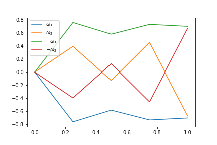
Figure 1: The approximate cubature paths in Example 7.6 (rescaling to $T=1$)

For the Euler scheme, we also set time discretization step $D=12$. Let $\widetilde{M}_{Euler}$ denote the sample size in Euler scheme, namely the number of simulated paths of the Brownian motion. Clearly both the approximate value $Y^{Euler}_{0}$ and the running time depend on $\widetilde{M}_{Euler}$, in particular, the latter is proportional to $\widetilde{M}_{Euler}$. Note that $Y^{Euler}_{0}$ is random. We repeat the Euler scheme $1000$ times, each with sample size $\widetilde{M}_{Euler}$, and obtain $Y^{Euler,i}_{0}$ and the corresponding Euler scheme errors $e^{Euler}_{i}:=|Y^{Euler,i}_{0}-Y^{true}_{0}|$, $1\leq i\leq 1000$. We shall use the sample median $e^{Euler}_{median}$ of $\{e^{Euler}_{i}\}_{1\leq i\leq 1000}$ to measure the accuracy of the Euler scheme. We can then compare $e^{cub}$ and $e^{Euler}_{median}$, and to have a more precise comparison, we will actually compute the percentile of the cubature error $e^{cub}$ among the Euler scheme errors $\{e^{Euler}_{i}\}_{1\leq i\leq 1000}$: $\alpha$-percentile means about $1000\times\alpha\%=10\alpha$ of $\{e^{Euler}_{i}\}_{1\leq i\leq 1000}$ are smaller than $e^{cub}$. So $50\%$ roughly means $e^{cub}=e^{Euler}_{median}$ and the two methods have the same accuracy; while $\alpha\%<50\%$ means that $e^{cub}<e^{Euler}_{median}$ and the cubature method has better accuracy: the smaller $\alpha\%$ is, the better the cubature method outperforms. Moreover, since $\{e^{Euler}_{i}\}_{1\leq i\leq 1000}$ are i.i.d., we may use the Normal approximation to compute the percentile. We will report their mean $e^{Euler}_{mean}:={1\over 1000}\sum_{i=1}^{1000}e^{Euler}_{i}\approx e^{Euler}_{median}$ and standard deviation $SD^{Euler}$, and then the percentile $\alpha\%\approx\Phi({e^{cub}-e^{Euler}_{mean}\over SD^{Euler}})$, where $\Phi$ is the cdf of the standard normal.

For the above example, we test three cases: $\widetilde{M}_{Euler}=100,500,1000$, and the numerical results are reported in Table 3. As we see, when $\widetilde{M}_{Euler}=500$, the Euler schemes takes $70$ milliseconds (for each run, not for $1000$ runs), which is about $38$ times slower than the $1.86$ milliseconds used for the cubature method, and the percentile of the cubature method is $24\%$. So the cubature method outperforms the Euler scheme both in running time and in accuracy. When we increase the sample size $\widetilde{M}_{Euler}$ to $1000$, the percentile increases to $27\%$, so the cubature method still outperforms in accuracy. In this case the running time of the Euler scheme increases to $141$ milliseconds, which is about $76$ times slower than the cubature method. On the other hand, if we decrease the sample size $\widetilde{M}_{Euler}$ to $100$, the running time of the Euler scheme drops to $14.2$ milliseconds, which is still $7.6$ times slower than the cubature method, but the accuracy deteriorates further with a percentile $19.4\%$. So in all three cases, the cubature method outperforms the Euler scheme significantly both in running time and in accuracy.

We conclude this subsection with an example concerning the impact of $D$.

Example 7.7.

Consider the same setting as in Example 7.6, but we try three different $D$’s. The numerical results are shown in Table 5.

$D$	$12$	$60$	$120$
$e^{cub}$ (cubature time)	$0.00046$ ($1.86$ms)	$0.00046$ ($15.3$ms)	$0.00046$ ($54.7$ms)
$e^{Euler}_{mean}$ (time, $\tilde{M}=100$)	$0.00338$ ($14.2$ms)	$0.0034$ ($314$ms)	$0.00336$ ($1.24$s)
$e^{Euler}_{mean}$ (time, $\tilde{M}=500$)	$0.00156$ ($70$ms)	$0.00161$ ($1.54$s)	$0.00108$ ($5.9$s)
$e^{Euler}_{mean}$ (time, $\tilde{M}=1000$)	$0.00114$ ($141$ms)	$0.00113$ ($3.11$s)	$0.00107$ ($11.5$s)

Table 5: The numerical results for Example 7.7

As we can see, the cubature method is not sensitive to $D$. The Euler scheme does rely on our choices of $D$ and $\tilde{M}_{Euler}$. However, in all the above choices, the cubature method outperforms both in running time and in accuracy.

7.3 A one dimensional nonlinear model

We now consider the following nonlinear model, but still in $1$-dimensional setting:

$$X_{t}=x_{0}+\int_{0}^{t}(t-r)^{H-{1\over 2}}\cos(X_{s})dB_{r},\quad Y_{0}=\mathbb{E}[G(X_{T})].$$ (7.5)

We shall use one period cubature method with $N=5$ when $T$ is small, and multiple period cubature method with $N=3$ and appropriate $M$ when $T$ is large. Our main purpose is to compare the efficiency of the cubature method with that of the Euler scheme.

We first note that, by Remark 7.1 (ii), the cubature paths for (7.5) is the same as those for (7.2). In particular, for the one period method with $N=5$, we may continue to use the paths in Table 4. For comparison purpose, we will use the same $D$ for the cubature method and the Euler scheme. For the $\widetilde{M}_{Euler}$ in Euler scheme, there is an obvious tradeoff between the running time and the accuracy. While one may try to find an “optimal” $\tilde{M}_{Euler}$ for a given $D$, such an analysis relies on a precise idea on the constants involved in the error estimates, as in Remark 7.2 (ii). Since our main focus is the cubature method and since our examples show that the cubature method outperforms significantly (under our strong conditions), we do not go through that analysis. Instead, unless stated otherwise, for simplicity in the rest of this section we shall always set

$$\widetilde{M}_{Euler}=500,\quad\mbox{and we repeat the Euler scheme for $1000$ times},$$

each time with $\widetilde{M}_{Euler}$ simulation paths. We use $\{Y^{Euler,i}_{0}\}_{1\leq i\leq 1000}$ and $Y^{true}_{0}$ to compute $e^{Euler}_{mean}$ and $SD^{Euler}$. However, in this case we are not able to compute the exact value of $Y^{true}_{0}$ as in (7.3). Since the convergence of the Euler scheme approximations is well understood, for comparison purpose we shall set the true value as the sample mean of the Euler scheme approximations:

$$Y^{true}_{0}={1\over 1000}\sum_{i=1}^{1000}Y^{Euler,i}_{0}.$$ (7.6)

In the first example we show the impact of the regularity of $G$.

Example 7.8.

Consider (7.5) with $H={3\over 2}$, $T=0.2$, and we consider three different $G$’s with corresponding $x_{0}$. We choose $D=12$, and compare the one period cubature method with $N=5$ with the Euler scheme. The numerical results are reported in Table 6.

$G(x)$ /  $x_{0}$	$\cos(x)$ /  1	$x^{2}$ /  1	$(x-0.5)^{+}$  /  0.56
$Y^{true}_{0}$	0.5401	1.00073	0.0617
$Y^{cub}_{0}$	0.5402	1.00041	0.0601
$e^{cub}$ (time)	0.0001(1.75ms)	0.00032(1.66ms)	0.0016 (1.63ms)
$e^{Euler}_{mean}$ (time)	0.0008(80.4ms)	0.00200(82ms )	0.00147(75ms)
$SD^{Euler}$(percentile)	0.00064(18%)	0.00149(20.1%)	0.0011(54.3%)

Table 6: The numerical results for Example 7.8

As we can see, the cubature method outperforms the Euler scheme in all these three cases. However, when $G$ becomes less smooth, the advantage of the cubature method fades away, which is consistent with the theoretical observation in Remark 2.8.

The next example illustrates the impact of $T$.

Example 7.9.

Consider (7.5) with $H={3\over 2}$, $G(x)=x^{2}$, $x_{0}=1$, and three different values of $T$: $0.2,\leavevmode\nobreak\ 0.5,\leavevmode\nobreak\ 0.8$. We choose $D=12,\leavevmode\nobreak\ 30,\leavevmode\nobreak\ 48$, respectively, and compare the one period cubature method with $N=5$ with the Euler scheme. The numerical results are reported in Table 7.

$T$	0.2	0.5	0.8
$Y^{true}_{0}$	1.00073	1.0109	1.045
$Y^{cub}_{0}$	1.00041	1.0056	1.022
$e^{cub}$ (time)	0.00032(1.66ms)	0.0054(5.25ms)	0.0234(11ms)
$e^{Euler}_{mean}$ (time)	0.00200 (82ms)	0.0332(445ms)	0.0152(1.16s)
$SD^{Euler}$(percentile)	0.00149(20.1%)	0.0098(57.4%)	0.0115(69.4%)

Table 7: The numerical results for Example 7.9

Again consistent with our theoretical result, the performance of the cubature method decays when $T$ gets large. In the above example, the cubature method obviously outperforms the Euler scheme when $T=0.2$, and still works better when $T=0.5$, but in the case $T=0.8$, there is a tradeoff between the speed and the accuracy and it is hard to claim the cubature method is more efficient. In the last case, we shall use the multiple period cubature method, as we do in the next example, and we can easily see that the cubature method outperforms the Euler scheme again.

Example 7.10.

Consider (7.5) with $H={3\over 2}$, $T=1$, and three different $G$’s with corresponding $x_{0}$. We choose $D=100$, and compare the multiple period cubature method with $M=5$ and $N=3$ with the Euler scheme. The numerical results are reported in Table 8.

$G(x)$ /  $x_{0}$	$\cos(x)$ /  1	$x^{2}$ /  1	$(x-0.5)^{+}$  /  0.56
$Y^{true}_{0}$	$0.5136$	$1.098$	$0.2275$
$Y^{mul,5}_{0}$	$0.5186$	$1.084$	$0.2297$
$e^{mul,5}$ (time)	$0.005(300ms)$	$0.014(302ms)$	$0.0022(302ms)$
$e^{Euler}_{mean}$ (time)	0.0074(4.2s)	0.023 ($4.36$s)	0.011 ($4.41$s)
$SD^{Euler}$(percentile)	$0.0056$ (37.37%)	$0.017$ ($35.1\%$)	$0.0089$ ($21\%$)

Table 8: The numerical results for Example 7.10

7.4 A fractional stochastic volatility model

In this section we consider the following special case of (6.3) with $H={3\over 2}$ and $\rho={1\over 2}$:

$$\left.\begin{array}[]{c}\displaystyle dS_{t}=S_{t}b_{1}(U_{t})dt+S_{t}\sigma_{1}(U_{t})\circ dB_{t}^{1},\vskip 6.0pt plus 2.0pt minus 2.0pt\\ \displaystyle U_{t}=1+\int_{0}^{t}[t-s][{1\over 2}-{1\over 3}U_{s}]ds+\int_{0}^{t}[t-s]\sigma_{2}(U_{s})\circ dB_{t}^{2},\\ \end{array}\right.$$ (7.9)

Again we will use one period cubature method with $N=5$ when $T$ is small, multiple period cubature method with $N=3$ and appropriate $M$ when $T$ is large, and we shall compare the efficiency between the cubature method and the Euler scheme.

Example 7.11.

Consider (7.9) with $T=0.1$, $b_{1}(U)=U$, $\sigma_{1}(U)=\sigma_{2}(U)=\cos(U)$, and we consider three different $G$’s with corresponding $S_{0}$. We choose $D=12$, and compare the one period cubature method with $N=5$ with the Euler scheme. The numerical results are reported in Table 9.

$G(x)$ /  $S_{0}$	$\cos(x)$ /  1	$x^{2}$ /  1	$(x-0.5)^{+}$  /  0.56
$Y^{true}_{0}$	$0.4270$	$1.2947$	$0.1320$
$Y^{cub}_{0}$	$0.4257$	$1.2967$	$0.1283$
$e^{cub}$ (time)	$0.0013(8.53ms)$	$0.0020(8.9ms)$	$0.0037(8.68ms)$
$e^{Euler}_{mean}$ (time)	0.0063 (273ms)	0.0157(283ms)	0.0037(272ms)
$SD^{Euler}$(percentile)	$0.0047$ (21.3%)	$0.0119$ ($19.2\%$)	$0.0028$ ($50\%$)

Table 9: The numerical results for Example 7.11

For the cubature method, we first compute the cubature paths following the same idea as in Remark 7.1. By §8.1 below we choose $W=5$ and $L=4$. Then we obtain

$$\lambda_{1}=0.0247245002,\quad\lambda_{2}=0.0561159547,\quad\lambda_{3}=0.417734596e,$$

$$\lambda_{4}=0.00142494883,\quad\lambda_{5}=4.44061201e-17$$

and the $10$ paths are plotted in Figure 2 (after rescaling to $T=1$).

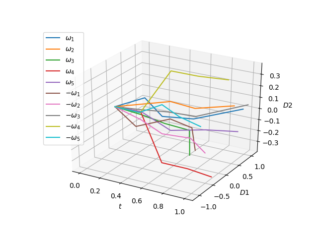
Figure 2: The cubature paths for the model (7.9) (rescaling to $T=1$)

Example 7.12.

Consider the same setting as in Example 7.11, except that $b_{1}(U)=\sigma_{1}(U)=\sigma_{2}(U)=\sqrt{U}$. The numerical results are reported in Table 10.

$G(x)$ /  $S_{0}$	$\cos(x)$ /  1	$x^{2}$ /  1	$(x-0.5)^{+}$  /  0.56
$Y^{true}_{0}$	0.37897	1.4932	0.17098
$Y^{cub}_{0}$	0.3698	1.4887	0.17797
$e^{cub}$ (time)	$0.00917(8.06ms)$	$0.0045(8.39ms)$	$0.00699(8.07ms)$
$e^{Euler}_{mean}$ (time)	0.0119(306ms)	0.0361(311ms)	0.007(304ms)
$SD^{Euler}$(percentile)	0.0092(40.8%)	0.0270(19.1%)	0.0052(50%)

Table 10: The numerical results for Example 7.12

We remark that Example 7.12 uses the same cubature paths as in Example 7.11.

Example 7.13.

Consider (7.9) with $T=1$, $b_{1}(U)=U$, $\sigma_{1}(U)=\sigma_{2}(U)=\cos(U)$, $G(x)=(x-1/2)^{+}$, $S_{0}=0.56$, and consider three different $H$. We shall compare the efficiency of the multiple period cubature method with $M=3$, $N=3$ and the Euler scheme. We set $D=100$. Recalling $\rho={1\over 2}$, for the cubature method we use $\theta_{1}=\frac{\pi}{6}$ and $\theta_{2}=-\frac{\pi}{6}$ in (6.16). We repeat the Euler scheme $100$ times (instead of $1000$ times). The numerical results are reported in Table 11.

$H$	$1$	$3/2$	$5/2$
$Y^{true}_{0}$	$1.36$	$1.33$	$1.2957$
$Y^{mul,3}_{0}$	$1.299$	$1.302$	$1.286$
$e^{mul,3}$(time)	$0.061(2.23s)$	$0.028(2.26s)$	$0.0097(2.42s)$
$e^{Euler}_{mean}$(time)	0.033 (15.8s)	0.036(15.8s)	0.037(15.5s)
$SD^{Euler}$(percentile)	$0.024$ (81.1%)	$0.028$ ($41.7\%$)	$0.0260$ ($21\%$)

Table 11: The numerical results for Example 7.13

We see that the cubature method outperforms the Euler scheme when $H={3\over 2}$ and $H={5\over 2}$, especially in the latter case, but does not seem to work well when $H=1$. This is consistent with our theoretical result.

7.5 Some concluding remarks

We first note that, our theoretical convergence analysis for the cubature method, namely Theorems 3.3 and 4.7, is complete, provided sufficient regularities on $K$ and $(V,G)$ (corresponding to $N$). In particular, it holds true for arbitrary dimensions and arbitrarily large $T$ (for Theorem 4.7).

For the numerical efficiency, in its realm, the cubature method has clear advantages over the Euler scheme. In light of Remark 4.8, the cubature method requires the following three conditions though: (i) sufficient regularity, so as to obtain the desired error estimate; (ii) low dimension (and relatively small $N$), so that $W$ can be relatively small; and (iii) not too large $T$, so that $M$ can be relatively small. We remark that the standard cubature method in [40] for diffusions also requires these conditions. However, the constraints are more severe in the Volterra setting here, for example, the constant $C_{N}$ in (4.33) is larger here, and for given dimensions and $N$, there are more equations required in (4.13) and hence we may need a larger $W$. When the number of cubature paths $(2W)^{M}$ is large (recalling again Remark 4.8 (ii)), it will be interesting to explore if the approach in [11, 12] could help reduce the complexity, which we shall leave for future research. The less smooth case, especially when $H<{1\over 2}$, requires novel idea to extend our approach.

We shall also remark that the parameters $M,N$ in the cubature method cannot be too big. For the Euler scheme, by increasing the sample size $\widetilde{M}_{Euler}$ gradually one may improve the accuracy “continuously” at the price of sacrificing the speed. For the cubature method we have only limited choices on $M,N$ and thus lose the flexibility of improving its accuracy “continuously”. Consequently, the cubature method is more appropriate in the situations where one has strong requirement on the speed but is less stringent on the accuracy.

8 Appendix

Proof of Proposition 2.4. Recall (2.8). Following rather standard arguments, we see that $\partial_{\bf x}u(t,\cdot)$ exists and has the following representation:

$$\left.\begin{array}[]{c}\displaystyle\langle\partial_{\bf x}u(t,\theta),\eta\rangle=\mathbb{E}\big{[}\partial_{x}G(X^{t,\theta}_{T})\cdot\nabla_{\eta}X^{t,\theta}_{T}\big{]},\quad\theta,\eta\in\mathbb{X}_{t},\vskip 6.0pt plus 2.0pt minus 2.0pt\\ \displaystyle\mbox{where}\quad\nabla_{\eta}X^{t,\theta,i}_{s}=\eta^{i}_{s}+\sum_{j=0}^{d}\int_{t}^{s}K_{i}(s,r)\partial_{x}V^{i}_{j}(X^{t,\theta}_{r})\nabla_{\eta}X^{t,\theta,j}_{r}\circ dB^{j}_{r},\quad i=1,\cdots,d_{1}.\end{array}\right.$$ (8.3)

We note that at above we need the second derivative of $V^{i}_{j}$ exists so that the Stratonovich integration $\circ$ makes sense. Then we see immediately $\|\partial_{\bf x}u(t,\theta)\|\leq Ce^{C^{m}_{N}(T-t)}$. By similar arguments we can prove the results for higher order derivatives. In particular, we note that the $(N-1)$-th derivative of $u$ would involve the $N$-th derivative of $V^{i}_{j}$.  

Proof of Proposition 2.5. We first note that, by Proposition 2.4 $u(t^{m}_{0},\cdot)\in C^{N+2}(\mathbb{X}_{t^{m}_{0}})$, so the right side of (2.20) makes sense.

When $N=1,2$, one may verify easily that (2.20) reduces to (2.10), (2.2), respectively. Assume (2.20) holds for $N-1$. For $\vec{i}\in{\cal I}_{N}$, $\vec{j}\in{\cal J}_{N}$, $\vec{\kappa}\in{\cal S}_{N}$, $\vec{t}\in\mathbb{T}_{N}$, we have

$$\displaystyle\Delta_{N+1}(\vec{i},\vec{j},\vec{\kappa};\vec{t}):={\cal V}(\vec{i},\vec{j},\vec{\kappa};\vec{t},\Theta^{\vec{t}}_{t_{N}},\Theta^{[t^{m}_{0},T]}_{t_{N}})-{\cal V}(\vec{i},\vec{j},\vec{\kappa};\vec{t},\Theta^{\vec{t}}_{T_{m}},\Theta^{[t^{m}_{0},T]}_{T_{m}})$$

$$\displaystyle=\prod_{\alpha=1}^{N}\partial^{\vec{\kappa},\alpha}_{\vec{i}}V^{i_{\alpha}}_{j_{\alpha}}(\Theta^{t_{\alpha}}_{t_{N}}){\cal K}_{+}(\vec{i},\vec{\kappa};\vec{t})\leavevmode\nobreak\ \big{\langle}\partial_{\vec{i}}^{\vec{\kappa}}u(t^{m}_{0},\Theta^{[t^{m}_{0},T]}_{t_{N}}),\vec{\cal K}_{0}(\vec{i},\vec{\kappa};\vec{t})\big{\rangle}$$

$$\displaystyle\quad-\prod_{\alpha=1}^{N}\partial^{\vec{\kappa},\alpha}_{\vec{i}}V^{i_{\alpha}}_{j_{\alpha}}(\Theta^{t_{\alpha}}_{T_{m}}){\cal K}_{+}(\vec{i},\vec{\kappa};\vec{t})\leavevmode\nobreak\ \big{\langle}\partial_{\vec{i}}^{\vec{\kappa}}u(t^{m}_{0},\Theta^{[t^{m}_{0},T]}_{T_{m}}),\vec{\cal K}_{0}(\vec{i},\vec{\kappa};\vec{t})\big{\rangle}.$$

Note that, for $s\in[T_{m},t_{N}]$, by Itô’s formula and Proposition 2.3 we have

$$\left.\begin{array}[]{lll}\displaystyle d\partial^{\vec{\kappa},\alpha}_{\vec{i}}V^{i_{\alpha}}_{j_{\alpha}}(\Theta^{t_{\alpha}}_{s})=\sum_{\tilde{i}=1}^{d_{1}}\sum_{\tilde{j}=0}^{d}\partial_{x_{\tilde{i}}}[\partial^{\vec{\kappa},\alpha}_{\vec{i}}V^{i_{\alpha}}_{j_{\alpha}}](\Theta^{t_{\alpha}}_{s})K_{\tilde{i}}(t_{\alpha},\tilde{t})V^{\tilde{i}}_{\tilde{j}}(X_{s})\circ dB^{\tilde{j}}_{s},\vskip 6.0pt plus 2.0pt minus 2.0pt\\ \displaystyle d\big{\langle}\partial_{\vec{i}}^{\vec{\kappa}}u(t^{m}_{0},\Theta^{[t^{m}_{0},T]}_{s}),\vec{\cal K}_{0}(\vec{i},\vec{\kappa};\vec{t})\big{\rangle}\vskip 6.0pt plus 2.0pt minus 2.0pt\\ \displaystyle=\sum_{\tilde{i}=1}^{d_{1}}\sum_{\tilde{j}=0}^{d}\big{\langle}\partial_{{\bf x}_{\tilde{i}}}\partial_{\vec{i}}^{\vec{\kappa}}u(t^{m}_{0},\Theta^{[t^{m}_{0},T]}_{s}),(\vec{\cal K}_{0}(\vec{i},\vec{\kappa};\vec{t}),K_{\tilde{i},s}^{[t^{m}_{0},T]})\big{\rangle}V^{\tilde{i}}_{\tilde{j}}(X_{s})\circ dB^{\tilde{j}}_{s}.\end{array}\right.$$ (8.7)

Then, by Itô’s formula we have, for given $\vec{i}\in{\cal I}_{N}$, $\vec{j}\in{\cal J}_{N}$, $\vec{t}\in\mathbb{T}_{N}$,

$$\displaystyle\Delta_{N+1}(\vec{i},\vec{j},\vec{\kappa};\vec{t})=\sum_{\tilde{i}=1}^{d_{1}}\sum_{\tilde{j}=0}^{d}\int_{T_{m}}^{t_{N}}\Xi_{N+1}\big{(}(\vec{i},\tilde{i}),(\vec{j},\tilde{j}),\vec{\kappa};(\vec{t},s)\big{)}\circ dB^{\tilde{j}}_{s},\quad\mbox{where}$$

$$\displaystyle\Xi_{N+1}\big{(}(\vec{i},\tilde{i}),(\vec{j},\tilde{j}),\vec{\kappa};(\vec{t},s)\big{)}:=\sum_{\tilde{\alpha}=1}^{N}\prod_{\alpha\in\{1,\cdots,N\}\backslash\{\tilde{\alpha}\}}\partial^{\vec{\kappa},\alpha}_{\vec{i}}V^{i_{\alpha}}_{j_{\alpha}}(\Theta^{t_{\alpha}}_{s})\times$$

$$\displaystyle\qquad\partial_{x_{\tilde{i}}}[\partial^{\vec{\kappa},\tilde{\alpha}}_{\vec{i}}V^{i_{\tilde{\alpha}}}_{j_{\tilde{\alpha}}}](\Theta^{t_{\tilde{\alpha}}}_{s})V^{\tilde{i}}_{\tilde{j}}(\Theta^{s}_{s}){\cal K}(\vec{i},\vec{\kappa};\vec{t})K_{\tilde{i}}(t_{\tilde{\alpha}},s)\leavevmode\nobreak\ \big{\langle}\partial_{\vec{i}}^{\vec{\kappa}}u(t^{m}_{0},\Theta^{[t^{m}_{0},T]}_{s}),\vec{\cal K}_{0}(\vec{i},\vec{\kappa};\vec{t})\big{\rangle}$$ (8.8)

$$\displaystyle\quad+\prod_{\alpha=1}^{N}\partial^{\vec{\kappa},\alpha}_{\vec{i}}V^{i_{\alpha}}_{j_{\alpha}}(\Theta^{t_{\alpha}}_{s})V^{\tilde{i}}_{\tilde{j}}(\Theta^{s}_{s}){\cal K}(\vec{i},\vec{\kappa};\vec{t})\leavevmode\nobreak\ \big{\langle}\partial_{{\bf x}_{\tilde{i}}}\partial_{\vec{i}}^{\vec{\kappa}}u(t^{m}_{0},\Theta^{[t^{m}_{0},T]}_{s}),(\vec{\cal K}_{0}(\vec{i},\vec{\kappa};\vec{t}),K_{\tilde{i},s}^{[t^{m}_{0},T]})\big{\rangle}.$$

Thus, since (2.20) holds for $N-1$ by induction assumption, we have

$$\displaystyle u(t^{m}_{0},\Theta^{[t^{m}_{0},T]}_{t^{m}_{0}})-u(t^{m}_{0},\Theta^{[t^{m}_{0},T]}_{T_{m}})$$

$$\displaystyle=\sum_{n=1}^{N-1}\sum_{\vec{i}\in{\cal I}_{n},\vec{j}\in{\cal J}_{n},\vec{\kappa}\in{\cal S}_{n}}\int_{\mathbb{T}^{m}_{n}}{\cal V}(\vec{i},\vec{j},\vec{\kappa};\vec{t},\Theta^{\vec{t}}_{T_{m}},\Theta^{[t^{m}_{0},T]}_{T_{m}})\circ dB_{\vec{t}}^{\vec{j}}$$

$$\quad+\sum_{\vec{i}\in{\cal I}_{N},\vec{j}\in{\cal J}_{N},\vec{\kappa}\in{\cal S}_{N}}\int_{\mathbb{T}^{m}_{N}}{\cal V}(\vec{i},\vec{j},\vec{\kappa};\vec{t},\Theta^{\vec{t}}_{t_{N}},\Theta^{[t^{m}_{0},T]}_{t_{N}})\circ dB_{\vec{t}}^{\vec{j}}$$

$$=\sum_{n=1}^{N}\sum_{\vec{i}\in{\cal I}_{n},\vec{j}\in{\cal J}_{n},\vec{\kappa}\in{\cal S}_{n}}\int_{\mathbb{T}^{m}_{n}}{\cal V}(\vec{i},\vec{j},\vec{\kappa};\vec{t},\Theta^{\vec{t}}_{T_{m}},\Theta^{[t^{m}_{0},T]}_{T_{m}})\circ dB_{\vec{t}}^{\vec{j}}$$

$$\displaystyle\quad+\sum_{(\vec{i},\tilde{i})\in{\cal I}_{N+1},(\vec{j},\tilde{j})\in{\cal J}_{N+1},\vec{\kappa}\in{\cal S}_{N}}\int_{\mathbb{T}^{m}_{N+1}}\Xi_{N+1}\big{(}(\vec{i},\tilde{i}),(\vec{j},\tilde{j}),\vec{\kappa};(\vec{t},s)\big{)}\circ dB_{(\vec{t},s)}^{(\vec{j},\tilde{j})}.$$

Then it suffices to show that,

$$\Xi_{N+1}\big{(}(\vec{i},\tilde{i}),(\vec{j},\tilde{j}),\vec{\kappa};(\vec{t},s)\big{)}=\sum_{\tilde{\alpha}=0}^{N}{\cal V}((\vec{i},\tilde{i}),(\vec{j},\tilde{j}),(\vec{\kappa},\tilde{\alpha});(\vec{t},s),\Theta^{(\vec{t},s)}_{s},\Theta^{[t^{m}_{0},T]}_{s}).$$ (8.9)

Indeed, recall (2.19), one can verify that

$$\displaystyle\Xi_{N+1}\big{(}(\vec{i},\tilde{i}),(\vec{j},\tilde{j}),\vec{\kappa};(\vec{t},s)\big{)}$$

$$\displaystyle=\sum_{\tilde{\alpha}=1}^{N}\prod_{\alpha=1}^{N}\partial^{(\vec{\kappa},\tilde{\alpha}),\alpha}_{(\vec{i},\tilde{i})}V^{i_{\alpha}}_{j_{\alpha}}(\Theta^{t_{\alpha}}_{s})V^{\tilde{i}}_{\tilde{j}}(\Theta^{s}_{s}){\cal K}((\vec{i},\tilde{i}),(\vec{\kappa},\tilde{\alpha});(\vec{t},s))\times$$

$$\displaystyle\qquad\qquad\qquad\big{\langle}\partial_{(\vec{i},\tilde{i})}^{(\vec{\kappa},\tilde{\alpha})}u(t^{m}_{0},\Theta^{[t^{m}_{0},T]}_{s}),\vec{\cal K}_{0}((\vec{i},\tilde{i}),(\vec{\kappa},\tilde{\alpha});(\vec{t},s))\big{\rangle}$$

$$\displaystyle\quad+\prod_{\alpha=1}^{N}\partial^{(\vec{\kappa},0),\alpha}_{(\vec{i},\tilde{i})}V^{i_{\alpha}}_{j_{\alpha}}(\Theta^{t_{\alpha}}_{s})V^{\tilde{i}}_{\tilde{j}}(\Theta^{s}_{s}){\cal K}((\vec{i},\tilde{i}),(\vec{\kappa},0);(\vec{t},s))\times$$

$$\displaystyle\qquad\qquad\qquad\big{\langle}\partial_{(\vec{i},\tilde{i})}^{(\vec{\kappa},0)}u(t^{m}_{0},\Theta^{[t^{m}_{0},T]}_{s}),(\vec{\cal K}_{0}((\vec{i},\tilde{i}),(\vec{\kappa},0);(\vec{t},s))\big{\rangle}$$

$$\displaystyle=\sum_{\tilde{\alpha}=0}^{N}\prod_{\alpha=1}^{N+1}\partial^{(\vec{\kappa},\tilde{\alpha}),\alpha}_{(\vec{i},\tilde{i})}V^{i_{\alpha}}_{j_{\alpha}}(\Theta^{t_{\alpha}}_{s}){\cal K}((\vec{i},\tilde{i}),(\vec{\kappa},\tilde{\alpha});(\vec{t},s))\times$$

$$\displaystyle\qquad\qquad\qquad\big{\langle}\partial_{(\vec{i},\tilde{i})}^{(\vec{\kappa},\tilde{\alpha})}u(t^{m}_{0},\Theta^{[t^{m}_{0},T]}_{s}),\vec{\cal K}_{0}((\vec{i},\tilde{i}),(\vec{\kappa},\tilde{\alpha});(\vec{t},s))\big{\rangle}$$

$$\displaystyle=\sum_{\tilde{\alpha}=0}^{N}{\cal V}((\vec{i},\tilde{i}),(\vec{j},\tilde{j}),(\vec{\kappa},\tilde{\alpha});(\vec{t},s),\Theta^{(\vec{t},s)}_{s},\Theta^{[t^{m}_{0},T]}_{s}).$$

This proves (8.9), hence (2.20) for $N$.  

Proof of Lemma 2.6. Recall that $B^{0}_{t}=t$, the case $j_{1}=0$ is obvious. We now assume $j_{1}>0$. Fix ${T_{m}}\leq s\leq t^{m}_{0}$ and denote

$$\psi(t_{1},t_{2}):=\int_{\mathbb{T}^{m}_{n-2}(t_{2})}\varphi(t_{1},t_{2},\vec{t}_{-2})\circ dB^{\vec{j}_{-2}}_{\vec{t}_{-2}}.$$

Then, when $j_{2}\neq j_{1}$, we have

$$\int_{\mathbb{T}^{m}_{n}(s)}\!\!\!\varphi(\vec{t}\leavevmode\nobreak\ \!)\circ dB^{\vec{j}}_{\vec{t}}=\int_{T_{m}}^{s}\Big{[}\int_{T_{m}}^{t_{1}}\psi(t_{1},t_{2})\circ dB^{j_{2}}_{t_{2}}\Big{]}\circ dB^{j_{1}}_{t_{1}}=\int_{T_{m}}^{s}\Big{[}\int_{T_{m}}^{t_{1}}\psi(t_{1},t_{2})\circ dB^{j_{2}}_{t_{2}}\Big{]}dB^{j_{1}}_{t_{1}},$$

coinciding with the Ito integral, and when $j_{1}=j_{2}$,

$$\int_{\mathbb{T}^{m}_{n}(s)}\!\!\!\varphi(\vec{t}\leavevmode\nobreak\ \!)\circ dB^{\vec{j}}_{\vec{t}}=\int_{T_{m}}^{s}\Big{[}\int_{T_{m}}^{t_{1}}\psi(t_{1},t_{2})\circ dB^{j_{2}}_{t_{2}}\Big{]}dB^{j_{1}}_{t_{1}}+{1\over 2}\int_{T_{m}}^{s}\psi(t_{1},t_{1})dt_{1}.$$

Then one may verify (2.26) and (2.30) straightforwardly.  

Proof of Theorem 2.7. First, similar to (2.2) and (2.20), one can verify that

$$\left.\begin{array}[]{c}\displaystyle R^{m}_{N}=\sum_{n=1}^{N+1}\sum_{\vec{i}\in{\cal I}_{n},\vec{j}\in{\cal J}_{n}}\big{[}{\bf 1}_{\{\|\vec{j}\|=N+1\}}+{\bf 1}_{\{\|\vec{j}_{-1}\|=N,j_{1}=0\}}\big{]}\times\\ \displaystyle\int_{\mathbb{T}^{m}_{n}}\sum_{\vec{\kappa}\in{\cal S}_{n}}{\cal V}(\vec{i},\vec{j},\vec{\kappa};\vec{t},\Theta^{\vec{t}}_{t_{n}},\Theta^{[t^{m}_{0},T]}_{t_{n}})\circ dB^{\vec{j}}_{\vec{t}}.\end{array}\right.$$ (8.12)

Fix $n$, $\vec{i}\in{\cal I}_{n}$, $\vec{j}\in{\cal J}_{n}$, and denote $\varphi(\vec{t}):=\sum_{\vec{\kappa}\in{\cal S}_{n}}{\cal V}(\vec{i},\vec{j},\vec{\kappa};\vec{t},\Theta^{\vec{t}}_{t_{n}},\Theta^{[t^{m}_{0},T]}_{t_{n}})$ for $\vec{t}\in\mathbb{T}^{m}_{n}$. By (2.30) and (2.33) we may prove by induction that, for $s\in[T_{m},t^{m}_{0}]$, $l=1,\cdots,n-1$, and for some constant $C_{n}$ which may depend on $n$,

$$\|\varphi(\cdot)\|_{s,\vec{j}}^{2} \leq C_{n}\delta^{\|\vec{j}_{l}\|}\mathop{\rm ess\;sup}_{T_{m}\leq s_{l}\leq\cdots\leq s_{1}\leq s}\|\varphi(s_{1},\cdots,s_{l},\cdot)\|_{\vec{j}_{-l},s_{l}}^{2}$$

$$+C_{n}\delta^{\|\vec{j}_{l+1}\|}\mathop{\rm ess\;sup}_{T_{m}\leq s_{l+1}\leq\cdots\leq s_{1}\leq s}\|\varphi(s_{1},\cdots,s_{l+1},\cdot)\|_{\vec{j}_{-l-1},s_{l+1}}^{2}$$

In particular, by setting $l=n-1$ we have

$$\displaystyle\mathbb{E}_{m}\Big{[}\Big{|}\int_{\mathbb{T}^{m}_{n}}\varphi(\vec{t})\circ dB^{\vec{j}}_{\vec{t}}\Big{|}^{2}\Big{]}\leq C_{n}[\Lambda_{n-1}+\Lambda_{n}],\quad\mbox{where}$$ (8.13)

$$\displaystyle\Lambda_{n-1}:=\delta^{\|\vec{j}_{n-1}\|}\mathop{\rm ess\;sup}_{\vec{s}\in\mathbb{T}^{m}_{n-1}}\mathbb{E}_{m}\Big{[}\Big{|}\int_{T_{m}}^{s_{n-1}}\varphi(\vec{s},t_{n})\circ dB^{j_{n}}_{t_{n}}\Big{|}^{2}\Big{]},\quad\Lambda_{n}:=\delta^{\|\vec{j}\|}\mathop{\rm ess\;sup}_{\vec{s}\in\mathbb{T}^{m}_{n}}\mathbb{E}_{m}\Big{[}\big{|}\varphi(\vec{s})\big{|}^{2}\Big{]}.$$

By (2.33) we have $\Lambda_{n}\leq|A^{m}_{\|\vec{j}\|}|^{2}\delta^{\|\vec{j}\|}$. Moreover, fix $\vec{s}\in\mathbb{T}_{n-1}$. When $j_{n}=0$, we have

$$\displaystyle\mathbb{E}_{m}\Big{[}\Big{|}\int_{T_{m}}^{s_{n-1}}\varphi(\vec{s},t_{n})\circ dB^{j_{n}}_{t_{n}}\Big{|}^{2}\Big{]}=\mathbb{E}_{m}\Big{[}\Big{|}\int_{T_{m}}^{s_{n-1}}\varphi(\vec{s},t_{n})d{t_{n}}\Big{|}^{2}\Big{]}$$

$$\displaystyle\leq\delta\mathbb{E}_{m}\Big{[}\int_{T_{m}}^{s_{n-1}}|\varphi(\vec{s},t_{n})|^{2}d{t_{n}}\Big{]}\leq\delta^{2}\mathop{\rm ess\;sup}_{T_{m}\leq t_{n}\leq s_{n-1}}\mathbb{E}_{m}\Big{[}|\varphi(\vec{s},t_{n})|^{2}\Big{]}\leq\delta^{2}|A^{m}_{\|\vec{j}\|}|^{2}.$$

Then

$$\Lambda_{n-1}\leq\delta^{\|\vec{j}_{n-1}\|}\delta^{2}|A^{m}_{\|\vec{j}\|}|^{2}=|A^{m}_{\|\vec{j}\|}|^{2}\delta^{\|\vec{j}\|}.$$

When $j_{n}>0$, recalling (2.19) and by (8.7) we have: denoting $s_{n}:=t_{n}$,

$$\displaystyle\int_{T_{m}}^{s_{n-1}}\varphi(\vec{s},t_{n})\circ dB^{j_{n}}_{t_{n}}$$

$$\displaystyle=\int_{T_{m}}^{s_{n-1}}\sum_{\vec{\kappa}\in{\cal S}_{n}}\prod_{\alpha=1}^{n}\partial^{\vec{\kappa},\alpha}_{\vec{i}}V^{i_{\alpha}}_{j_{\alpha}}(\Theta^{s_{\alpha}}_{t_{n}}){\cal K}_{+}(\vec{i},\vec{\kappa};(\vec{s},t_{n}))\leavevmode\nobreak\ \big{\langle}\partial_{\vec{i}}^{\vec{\kappa}}u(t^{m}_{0},\Theta^{[t^{m}_{0},T]}_{t_{n}}),\vec{\cal K}_{0}(\vec{i},\vec{\kappa};(\vec{s},t_{n}))\big{\rangle}\circ dB^{j_{n}}_{t_{n}}$$

$$\displaystyle=\int_{T_{m}}^{s_{n-1}}\sum_{\vec{\kappa}\in{\cal S}_{n}}\prod_{\alpha=1}^{n}\partial^{\vec{\kappa},\alpha}_{\vec{i}}V^{i_{\alpha}}_{j_{\alpha}}(\Theta^{s_{\alpha}}_{t_{n}}){\cal K}_{+}(\vec{i},\vec{\kappa};(\vec{s},t_{n}))\leavevmode\nobreak\ \big{\langle}\partial_{\vec{i}}^{\vec{\kappa}}u(t^{m}_{0},\Theta^{[t^{m}_{0},T]}_{t_{n}}),\vec{\cal K}_{0}(\vec{i},\vec{\kappa};(\vec{s},t_{n}))\big{\rangle}dB^{j_{n}}_{t_{n}}$$

$$\displaystyle+{1\over 2}\int_{T_{m}}^{s_{n-1}}\sum_{\vec{\kappa}\in{\cal S}_{n}}\Big{[}\sum_{\tilde{\alpha}=1}^{n}\prod_{\alpha\neq\tilde{\alpha}}\partial^{\vec{\kappa},\alpha}_{\vec{i}}V^{i_{\alpha}}_{j_{\alpha}}(\Theta^{s_{\alpha}}_{t_{n}}){\cal K}_{+}(\vec{i},\vec{\kappa};(\vec{s},t_{n}))\leavevmode\nobreak\ \big{\langle}\partial_{\vec{i}}^{\vec{\kappa}}u(t^{m}_{0},\Theta^{[t^{m}_{0},T]}_{t_{n}}),\vec{\cal K}_{0}(\vec{i},\vec{\kappa};(\vec{s},t_{n}))\big{\rangle}\times$$

$$\displaystyle\qquad\qquad\qquad\sum_{\tilde{i}=1}^{d_{1}}\big{[}\partial_{x_{\tilde{i}}}\partial^{\vec{\kappa},\tilde{\alpha}}_{\vec{i}}V^{i_{\tilde{\alpha}}}_{j_{\tilde{\alpha}}}(\Theta^{s_{\tilde{\alpha}}}_{t_{n}})K_{\tilde{i}}(s_{\tilde{\alpha}},t_{n})V^{\tilde{i}}_{j_{n}}(X_{t_{n}})]$$

$$\displaystyle\qquad\qquad+\prod_{\alpha=1}^{n}\partial^{\vec{\kappa},\alpha}_{\vec{i}}V^{i_{\alpha}}_{j_{\alpha}}(\Theta^{s_{\alpha}}_{t_{n}}){\cal K}_{+}(\vec{i},\vec{\kappa};(\vec{s},t_{n}))\times$$

$$\displaystyle\qquad\qquad\qquad\sum_{\tilde{i}=1}^{d_{1}}\leavevmode\nobreak\ \big{\langle}\partial_{{\bf x}_{\tilde{i}}}\partial_{\vec{i}}^{\vec{\kappa}}u(t^{m}_{0},\Theta^{[t^{m}_{0},T]}_{t_{n}}),(\vec{\cal K}_{0}(\vec{i},\vec{\kappa};(\vec{s},t_{n})),K_{\tilde{i},t_{n}}^{[t^{m}_{0},T]})\big{\rangle}V^{\tilde{i}}_{j_{n}}(X_{t_{n}})\Big{]}dt_{n}$$

$$\displaystyle=\int_{T_{m}}^{s_{n-1}}\sum_{\vec{\kappa}\in{\cal S}_{n}}\prod_{\alpha=1}^{n}\partial^{\vec{\kappa},\alpha}_{\vec{i}}V^{i_{\alpha}}_{j_{\alpha}}(\Theta^{s_{\alpha}}_{t_{n}}){\cal K}_{+}(\vec{i},\vec{\kappa};(\vec{s},t_{n}))\leavevmode\nobreak\ \big{\langle}\partial_{\vec{i}}^{\vec{\kappa}}u(t^{m}_{0},\Theta^{[t^{m}_{0},T]}_{t_{n}}),\vec{\cal K}_{0}(\vec{i},\vec{\kappa};(\vec{s},t_{n}))\big{\rangle}dB^{j_{n}}_{t_{n}}$$

$$\displaystyle\quad+{1\over 2}\sum_{\tilde{i}=1}^{d_{1}}\int_{T_{m}}^{s_{n-1}}\sum_{\vec{\kappa}\in{\cal S}_{n}}\sum_{\tilde{\alpha}=0}^{n}{\cal V}\big{(}(\vec{i},\tilde{i}),(\vec{j},j_{n}),(\vec{\kappa},\tilde{\alpha});(\vec{s},t_{n},t_{n}),\Theta^{(\vec{s},t_{n},t_{n})}_{t_{n}},\Theta^{[t^{m}_{0},T]}_{t_{n}}\big{)}dt_{n},$$

where, similarly to (8), the last equality can be verified straightforwardly. Then

$$\displaystyle\mathbb{E}_{m}\Big{[}\Big{|}\int_{T_{m}}^{s_{n-1}}\varphi(\vec{s},t_{n})\circ dB^{j_{n}}_{t_{n}}\Big{|}^{2}\Big{]}\leq C\delta|A^{m}_{\|\vec{j}\|}|^{2}+C\delta^{2}|A^{m}_{\|(\vec{j},j_{n})\|}|^{2}.$$

Thus

$$\Lambda_{n-1}\leq C\delta^{\|\vec{j}_{n-1}\|}\big{[}\delta|A^{m}_{\|\vec{j}\|}|^{2}+\delta^{2}|A^{m}_{\|(\vec{j},j_{n})\|}|^{2}\big{]}=C\big{[}|A^{m}_{\|\vec{j}\|}|^{2}\delta^{\|\vec{j}\|}+|A^{m}_{\|\vec{j}\|+1}|^{2}\delta^{\|\vec{j}\|+1}\big{]}.$$

So in all the cases, by (8.13) we have

$$\mathbb{E}_{m}\Big{[}\Big{|}\int_{\mathbb{T}^{m}_{n}}\varphi(\vec{t})\circ dB^{\vec{j}}_{\vec{t}}\Big{|}^{2}\Big{]}\leq C_{n}\Big{[}|A^{m}_{\|\vec{j}\|}|^{2}\delta^{\|\vec{j}\|}+|A^{m}_{\|\vec{j}\|+1}|^{2}\delta^{\|\vec{j}\|+1}\Big{]}.$$

Then, by (8.12) we obtain

$$\mathbb{E}_{m}[|R^{m}_{N}|^{2}]\leq C_{N}\sum_{n=1}^{N+1}\sum_{\vec{i}\in{\cal I}_{n},\vec{j}\in{\cal J}_{n}}\big{[}{\bf 1}_{\{\|\vec{j}\|=N+1\}}+{\bf 1}_{\{\|\vec{j}_{-1}\|=N,j_{1}=0\}}\big{]}\Big{[}|A^{m}_{\|\vec{j}\|}|^{2}\delta^{\|\vec{j}\|}+|A^{m}_{\|\vec{j}\|+1}|^{2}\delta^{\|\vec{j}\|+1}\Big{]}.$$

This implies (2.37) immediately.  

Proof of Theorem 3.3. It is clear that the functional Itô formula (2.7) holds true under $Q$ as well, then (3.12) and (8.12) also hold true under $Q$. Thus, by (3.19),

$$\big{|}Y_{0}-Y^{Q}_{0}\big{|}=\Big{|}\mathbb{E}[R_{N}]-\mathbb{E}^{Q}[R_{N}]\Big{|}.$$

Therefore, by Theorem 2.7, it suffices to show that

$$\big{|}\mathbb{E}^{Q}[R_{N}]\big{|}\leq C_{N}\Big{[}A_{N+1}T^{N+1\over 2}\big{(}1+C_{Q}^{N-1}\big{)}+A_{N+2}T^{N+2\over 2}\big{(}1+C_{Q}^{N-2}\big{)}\Big{]}.$$ (8.14)

Now for each $n$ and $\vec{i}\in{\cal I}_{n}$, $\vec{j}\in{\cal J}_{n}$ as in (8.12), note that

$$(\omega_{k,t}^{0})^{\prime}=1,\quad|\{l:j_{l}=0\}|=\|\vec{j}\|-n,\quad|\{l:j_{l}>0\}|=2n-\|\vec{j}\|,$$

where $\omega^{\prime}$ denotes the time derivative of $\omega$. Then

$$\displaystyle\Big{|}\mathbb{E}^{Q}\Big{[}\int_{\mathbb{T}_{n}}\sum_{\vec{\kappa}\in{\cal S}_{n}}{\cal V}(\vec{i},\vec{j},\vec{\kappa};\vec{t},\Theta^{\vec{t}}_{t_{n}},\Theta^{T}_{t_{n}})\circ dB^{\vec{j}}_{\vec{t}}\Big{]}\Big{|}\leq A_{\|\vec{j}\|}\sum_{k=1}^{2W}\lambda_{k}\int_{\mathbb{T}_{n}}\prod_{l=1}^{n}|(\omega^{j_{l}}_{k,t_{l}})^{\prime}|dt_{n}\cdots dt_{1}\Big{|}$$

$$\displaystyle\leq C_{n}A_{\|\vec{j}\|}\sum_{k=1}^{2W}\lambda_{k}({C_{Q}\over\sqrt{T}})|^{2n-\|\vec{j}\|}T^{n}=C_{n}A_{\|\vec{j}\|}C_{Q}^{2n-\|\vec{j}\|}T^{\|\vec{j}\|}.$$ (8.15)

If $\|\vec{j}\|=N+1$, we have $2n\geq N+1$. Denote $k:=2n-(N+1)$, then $0\leq k\leq N-1$, and

$$A_{\|\vec{j}\|}|C_{Q}|^{2n-\|\vec{j}\|}T^{\|\vec{j}\|}=A_{N+1}T^{N+1\over 2}C_{Q}^{k}.$$

If $\|\vec{j}_{-1}\|=N$, $j_{1}=0$, then $2n\geq N+2$. Denote $k:=2n-(N+2)$, then $0\leq k\leq N-2$, and

$$A_{\|\vec{j}\|}C_{Q}^{2n-\|\vec{j}\|}T^{\|\vec{j}\|}=A_{N+2}T^{N+2\over 2}C_{Q}^{k}.$$

Plug these into (8), we obtain (8.14) immediately, and hence (3.24) holds true.

Finally, when (3.25) holds true, by (3.19) one can easily see that $Q$ in (3.16) is an N-Volterra cubature formula on $[0,T]$ if and only if the following rescaled one $\tilde{Q}$ is an N-Volterra cubature formula on $[0,1]$:

$$\tilde{Q}=\sum_{k=1}^{2W}\lambda_{k}\delta_{\tilde{\omega}_{t}},\qquad d\tilde{\omega}_{k,t}=a_{k,l}dt,\leavevmode\nobreak\ t\in(\tilde{s}_{l-1},\tilde{s}_{l}],\qquad\tilde{s}_{l}:={l\over L},\quad l=0,\cdots,L.$$ (8.16)

In particular, this implies that $C_{Q}=C_{\tilde{Q}}$ is independent of $T$,  

Proof of Theorem 4.5. Note that

$$\displaystyle\Big{|}\mathbb{E}^{Q_{m}}_{m}\big{[}u(T_{m+1},\Theta^{[T_{m+1},T]}_{T_{m+1}}\big{]}-\mathbb{E}_{m}\big{[}u(T_{m+1},\Theta^{[T_{m+1},T]}_{T_{m+1}}\big{]}\Big{|}$$

$$\displaystyle\leq\Big{|}\mathbb{E}^{Q_{m}}_{m}[I^{m}_{N}]-\mathbb{E}_{m}[I^{m}_{N}]\Big{|}+\big{|}\mathbb{E}^{Q_{m}}_{m}[R^{m}_{N}]\big{|}+\big{|}\mathbb{E}_{m}[R^{m}_{N}]\big{|}.$$

Then, following the same arguments as in Theorem 3.3, it suffices to provide desired estimate for $\Big{|}\mathbb{E}^{Q_{m}}_{m}[I^{m}_{N}]-\mathbb{E}_{m}[I^{m}_{N}]\Big{|}$. Similar to Lemma 3.4, by the desired symmetric properties, for any $\vec{j}\in{\cal J}_{n,N}\backslash\bar{\cal J}_{n,N}$ we have

$$\mathbb{E}^{Q_{m}}_{m}\Big{[}\int_{\mathbb{T}^{m}_{n}}{\cal V}(\vec{i},\vec{j},\vec{\kappa};\vec{t},\Theta^{\vec{t}}_{T_{m}},\Theta^{[t^{m}_{0},T]}_{T_{m}})\circ dB^{\vec{j}}_{\vec{t}}\Big{]}=0=\mathbb{E}_{m}\Big{[}\int_{\mathbb{T}^{m}_{n}}{\cal V}(\vec{i},\vec{j},\vec{\kappa};\vec{t},\Theta^{\vec{t}}_{T_{m}},\Theta^{[t^{m}_{0},T]}_{T_{m}})\circ dB^{\vec{j}}_{\vec{t}}\Big{]}.$$

Then, by (4.13) we have

$$\Big{|}\mathbb{E}^{Q_{m}}_{m}[I^{m}_{N}]-\mathbb{E}_{m}[I^{m}_{N}]\Big{|}=\Big{|}\mathbb{E}^{Q_{m}}_{m}[\check{R}^{m}_{N}]-\mathbb{E}_{m}[\check{R}^{m}_{N}]\Big{|}\leq\Big{|}\mathbb{E}^{Q_{m}}_{m}[\check{R}^{m}_{N}]\Big{|}+\Big{|}\mathbb{E}_{m}[\check{R}^{m}_{N}]\Big{|}.$$

The estimate for $\Big{|}\mathbb{E}_{m}[\check{R}^{m}_{N}]\Big{|}$ is implied by (4.8). Moreover, for each $n\leq N$ and $\vec{j}\in\bar{\cal J}_{n,N}$, again set $k:={N-\|\vec{j}\|-1\over 2}$ as in the proof of Theorem 4.2. Then, by (4.6) and similar to (8),

$$\Big{|}\mathbb{E}^{Q_{m}}_{m}\Big{[}\int_{\mathbb{T}^{m}_{n}}\check{R}^{m}_{N}(\vec{t})\circ dB^{\vec{j}}_{\vec{t}}\Big{]}\Big{|}\leq C^{m}_{N}C_{Q_{m}}^{2n-\|\vec{j}\|}e^{C^{m}_{N}T}\delta^{N+1\over 2}.$$

Thus, since $0\leq 2n-\|\vec{j}\|\leq N-1$,

$$\Big{|}\mathbb{E}^{Q_{m}}_{m}[\check{R}^{m}_{N}]\Big{|}\leq\sum_{n=1}^{N}\sum_{\vec{j}\in\bar{\cal J}_{n,N}}C^{m}_{N}C_{Q_{m}}^{2n-\|\vec{j}\|}e^{C^{m}_{N}T}\delta^{N+1\over 2}\leq C^{m}_{N}\big{(}1+C_{Q_{m}}^{N-1}\big{)}e^{C^{m}_{N}T}\delta^{N+1\over 2}.$$

Recall $C_{Q_{m}}=C_{Q^{*}_{N}}$, this is the desired estimate.  

8.1 The one period cubature formula for (6.3) with $N=5$

Denote

$$\gamma_{1}:={T^{H_{+}+1}\over H_{+}(H_{+}+1)},\quad\gamma_{2}:={T^{2H_{+}}\over 8HH_{+}}.$$ (8.17)

First, similar to (3.6) we have

$$\displaystyle\tilde{b}_{1}(\Theta^{t_{1}}_{t_{1}})\displaystyle = R_{\neq 2}+\int_{0}^{t_{1}}\Big{[}\partial_{0}\tilde{b}_{1}(\Theta^{t_{1}}_{t_{2}})+\sum_{i=1}^{2}\partial_{i}\tilde{b}_{1}(\Theta^{t_{1}}_{t_{2}})b_{i}(\Theta^{t_{2}}_{t_{2}})K_{i}(t_{1},t_{2})\Big{]}dt_{2}$$

$$\displaystyle+\int_{0}^{t_{1}}\int_{0}^{t_{2}}\sum_{i,j=1}^{2}\Big{[}\partial_{ji}\tilde{b}_{1}(\Theta^{t_{1}}_{t_{3}})\sigma_{i}(\Theta^{t_{2}}_{t_{3}})K_{j}(t_{1},t_{3})$$

$$\displaystyle\quad+\partial_{i}\tilde{b}_{1}(\Theta^{t_{1}}_{t_{3}})\partial_{j}\sigma_{i}(\Theta^{t_{2}}_{t_{3}})K_{j}(t_{2},t_{3})\Big{]}\sigma_{j}(\Theta^{t_{3}}_{t_{3}})K_{i}(t_{1},t_{2})\circ dB^{j}_{t_{3}}\circ dB^{i}_{t_{2}}.$$

We remark that $\partial_{i}\tilde{b}_{1}=G^{\prime\prime}b_{1}+G^{\prime}\partial_{i}b_{1}$, however, thanks to the new convention in Remark 6.1, we do not need to consider $G^{\prime\prime}b_{1}$ and $G^{\prime}\partial_{i}b_{1}$ separately. Then we can easily see that the terms in $\Delta\tilde{\mathbb{V}}^{0}_{4}$ derived from $\tilde{b}_{1}$ consist of the following stochastic integrals:

$$\left.\begin{array}[]{c}\displaystyle\Delta\tilde{\mathbb{V}}^{0}_{4,b}:=\Big{\{}\tilde{\Gamma}_{4,b}^{(i,j,k)}:(i,j,k)=(1,1,1),(1,2,1),(1,2,2),(2,1,1),(2,2,1),(2,2,2)\Big{\}},\\ \displaystyle\mbox{where}\quad\tilde{\Gamma}_{4,b}^{(i,j,k)}:=\int_{\mathbb{T}_{3}}K_{i}(t_{1},t_{2})K_{j}(t_{k},t_{3})\circ dB^{j}_{t_{3}}\circ dB^{i}_{t_{2}}dt_{1}.\end{array}\right.$$ (8.21)

Note that, for $i,j,k=1,2$,

$$\displaystyle\mathbb{E}\big{[}\tilde{\Gamma}_{4,b}^{(i,j,k)}\big{]}={1\over 2}\int_{\mathbb{T}_{2}}K_{i}(t_{1},t_{2})K_{j}(t_{k},t_{2})d\langle B^{i},B^{j}\rangle_{t_{2}}dt_{1}=\left\{\begin{array}[]{lll}{T^{2}\over 4},&(i,j,k)=(1,1,1),\\ {\rho\gamma_{1}\over 2},&(i,j,k)=(1,2,1),(2,1,1),\\ \gamma_{2},&(i,j,k)=(2,2,1),\\ 0,&(i,j,k)=(1,2,2),(2,2,2).\end{array}\right.$$ (8.26)

Similarly, we may have the expansion of $\tilde{\sigma}_{1}(\Theta^{t_{1}}_{t_{1}})$ as in (8.1):

$$\displaystyle\tilde{\sigma}_{1}(\Theta^{t_{1}}_{t_{1}})=R_{\neq 3}+\sum_{i_{2}=1}^{2}\int_{0}^{t_{1}}\int_{0}^{t_{2}}\partial_{i_{2}0}\tilde{\sigma}_{1}(\Theta^{t_{1}}_{t_{3}})\sigma_{i_{2}}(\Theta^{t_{3}}_{t_{3}})K_{i_{2}}(t_{1},t_{3})\circ dB^{i_{2}}_{t_{3}}dt_{2}$$

$$\displaystyle+\sum_{i_{1},i_{2}=1}^{2}\int_{0}^{t_{1}}\int_{0}^{t_{2}}\Big{[}\partial_{i_{2}i_{1}}\tilde{\sigma}_{1}(\Theta^{t_{1}}_{t_{3}})b_{i_{1}}(\Theta^{t_{2}}_{t_{3}})K_{i_{2}}(t_{1},t_{3})$$

$$\displaystyle\qquad+\partial_{i_{1}}\tilde{\sigma}_{1}(\Theta^{t_{1}}_{t_{3}})\partial_{i_{2}}b_{i_{1}}(\Theta^{t_{2}}_{t_{3}})K_{i_{2}}(t_{2},t_{3})\Big{]}\sigma_{i_{2}}(\Theta^{t_{3}}_{t_{3}})K_{i_{1}}(t_{1},t_{2})\circ dB^{i_{2}}_{t_{3}}dt_{2}$$ (8.27)

$$\displaystyle+\sum_{i_{1}=1}^{2}\int_{0}^{t_{1}}\int_{0}^{t_{2}}\Big{[}\partial_{0i_{1}}\tilde{\sigma}_{1}(\Theta^{t_{1}}_{t_{3}})\sigma_{i_{1}}(\Theta^{t_{2}}_{t_{3}})+\partial_{i_{1}}\tilde{\sigma}_{1}(\Theta^{t_{1}}_{t_{3}})\partial_{0}\sigma_{i_{1}}(\Theta^{t_{2}}_{t_{3}})\Big{]}K_{i_{1}}(t_{1},t_{2})dt_{3}\circ dB^{i_{1}}_{t_{2}}$$

$$\displaystyle+\sum_{i_{1},i_{2}=1}^{2}\int_{0}^{t_{1}}\int_{0}^{t_{2}}\Big{[}\partial_{i_{2}i_{1}}\tilde{\sigma}_{1}(\Theta^{t_{1}}_{t_{3}})b_{i_{2}}(\Theta_{t_{3}}^{t_{3}})\sigma_{i_{1}}(\Theta^{t_{2}}_{t_{3}})K_{i_{2}}(t_{1},t_{3})$$

$$\displaystyle\qquad+\partial_{i_{1}}\tilde{\sigma}_{1}(\Theta^{t_{1}}_{t_{3}})\partial_{i_{2}}\sigma_{i_{1}}(\Theta^{t_{2}}_{t_{3}})b_{i_{2}}(\Theta_{t_{3}}^{t_{3}})K_{i_{2}}(t_{2},t_{3})\Big{]}K_{i_{1}}(t_{1},t_{2})dt_{3}\circ dB^{i_{1}}_{t_{2}}+\xi,$$

where the terms presented above involve $\partial_{t}$, and $\xi$ contains the terms without $\partial_{t}$:

$$\displaystyle\xi:=\sum_{i_{1},i_{2},i_{3}=1}^{2}\int_{0}^{t_{1}}\int_{0}^{t_{2}}\int_{0}^{t_{3}}\Big{[}\partial_{i_{3}i_{2}i_{1}}\tilde{\sigma}_{1}(\Theta^{t_{1}}_{t_{4}})\sigma_{i_{1}}(\Theta^{t_{2}}_{t_{4}})\sigma_{i_{2}}(\Theta^{t_{3}}_{t_{4}})K_{i_{2}}(t_{1},t_{3})K_{i_{3}}(t_{1},t_{4})$$

$$\displaystyle\qquad+\partial_{i_{2}i_{1}}\tilde{\sigma}_{1}(\Theta^{t_{1}}_{t_{4}})\partial_{i_{3}}\sigma_{i_{1}}(\Theta^{t_{2}}_{t_{4}})\sigma_{i_{2}}(\Theta^{t_{3}}_{t_{4}})K_{i_{2}}(t_{1},t_{3})K_{i_{3}}(t_{2},t_{4})$$

$$\displaystyle\qquad+\partial_{i_{2}i_{1}}\tilde{\sigma}_{1}(\Theta^{t_{1}}_{t_{4}})\sigma_{i_{1}}(\Theta^{t_{2}}_{t_{4}})\partial_{i_{3}}\sigma_{i_{2}}(\Theta^{t_{3}}_{t_{4}})K_{i_{2}}(t_{1},t_{3})K_{i_{3}}(t_{3},t_{4})$$

$$\displaystyle\qquad+\partial_{i_{3}i_{1}}\tilde{\sigma}_{1}(\Theta^{t_{1}}_{t_{4}})\partial_{i_{2}}\sigma_{i_{1}}(\Theta^{t_{2}}_{t_{4}})\sigma_{i_{2}}(\Theta^{t_{3}}_{t_{4}})K_{i_{2}}(t_{2},t_{3})K_{i_{3}}(t_{1},t_{4})$$ (8.28)

$$\displaystyle\qquad+\partial_{i_{1}}\tilde{\sigma}_{1}(\Theta^{t_{1}}_{t_{4}})\partial_{i_{3}i_{2}}\sigma_{i_{1}}(\Theta^{t_{2}}_{t_{4}})\sigma_{i_{2}}(\Theta^{t_{3}}_{t_{4}})K_{i_{2}}(t_{2},t_{3})K_{i_{3}}(t_{2},t_{4})$$

$$\displaystyle\qquad+\partial_{i_{1}}\tilde{\sigma}_{1}(\Theta^{t_{1}}_{t_{4}})\partial_{i_{2}}\sigma_{i_{1}}(\Theta^{t_{2}}_{t_{4}})\partial_{i_{3}}\sigma_{i_{2}}(\Theta^{t_{3}}_{t_{4}})K_{i_{2}}(t_{2},t_{3})K_{i_{3}}(t_{3},t_{4})\Big{]}\times$$

$$\displaystyle\qquad\sigma_{i_{3}}(\Theta^{t_{4}}_{t_{4}})K_{i_{1}}(t_{1},t_{2})\circ dB^{i_{3}}_{t_{4}}\circ dB^{i_{2}}_{t_{3}}\circ dB^{i_{1}}_{t_{2}}.$$

Then we see that the terms in $\Delta\tilde{\mathbb{V}}^{0}_{4}$ derived from $\tilde{\sigma}_{1}$ are:

$$\left.\begin{array}[]{lll}\displaystyle\Delta\tilde{\mathbb{V}}^{0}_{4,\sigma}=\Delta\tilde{\mathbb{V}}^{0}_{4,\sigma,0}\cup\Delta\tilde{\mathbb{V}}^{0}_{4,\sigma,1}\cup\Delta\tilde{\mathbb{V}}^{0}_{4,\sigma,2}\cup\Delta\tilde{\mathbb{V}}^{0}_{4,\sigma,3},\quad\mbox{where, for}\leavevmode\nobreak\ l=1,2,\vskip 6.0pt plus 2.0pt minus 2.0pt\\ \displaystyle\Delta\tilde{\mathbb{V}}^{0}_{4,\sigma,0}:=\Big{\{}\tilde{\Gamma}^{(1)}_{4,\sigma,0},\tilde{\Gamma}^{(2)}_{4,\sigma,0}\Big{\}},\vskip 6.0pt plus 2.0pt minus 2.0pt\\ \displaystyle\Delta\tilde{\mathbb{V}}^{0}_{4,\sigma,l}:=\Big{\{}\tilde{\Gamma}^{(i_{1},i_{2},\kappa_{2})}_{4,\sigma,l}:(i_{1},i_{2},\kappa_{2})=(1,1,1),(1,2,1),(1,2,2),(2,1,1),(2,2,1),(2,2,2)\Big{\}},\vskip 6.0pt plus 2.0pt minus 2.0pt\\ \end{array}\right.$$ (8.32)

and

$$\left.\begin{array}[]{lll}\displaystyle\Delta\tilde{\mathbb{V}}^{0}_{4,\sigma,3}:=\Big{\{}\tilde{\Gamma}^{(i_{1},i_{2},i_{3},\kappa_{2},\kappa_{3})}_{4,\sigma,3}:(i_{1},i_{2},i_{3},\kappa_{2},\kappa_{3})=(1,1,1,1,1),(1,1,2,1,1),\\ \displaystyle\qquad(1,1,2,1,2),(1,1,2,1,3),(1,2,1,1,1),(1,2,1,2,1),(1,2,2,1,1),(1,2,2,1,2),\\ \displaystyle\qquad(1,2,2,1,3),(1,2,2,2,1),(1,2,2,2,2),(1,2,2,2,3),(2,1,1,1,1),(2,1,2,1,1),\\ \displaystyle\qquad(2,1,2,1,2),(2,1,2,1,3),(2,2,1,1,1),(2,2,1,2,1),(2,2,2,1,1),(2,2,2,1,2),\\ \displaystyle\qquad(2,2,2,1,3),(2,2,2,2,1),(2,2,2,2,2),(2,2,2,2,3)\Big{\}},\end{array}\right.$$ (8.38)

where

$$\left.\begin{array}[]{lll}\displaystyle\tilde{\Gamma}^{(i_{2})}_{4,\sigma,0}:=\int_{\mathbb{T}_{3}}K_{i_{2}}(t_{1},t_{3})\circ dB^{i_{2}}_{t_{3}}dt_{2}\circ dB^{1}_{t_{1}},\vskip 6.0pt plus 2.0pt minus 2.0pt\\ \displaystyle\tilde{\Gamma}^{(i_{1},i_{2},\kappa_{2})}_{4,\sigma,1}:=\int_{\mathbb{T}_{3}}K_{i_{1}}(t_{1},t_{2})K_{i_{2}}(t_{\kappa_{2}},t_{3})\circ dB^{i_{2}}_{t_{3}}dt_{2}\circ dB^{1}_{t_{1}},\vskip 6.0pt plus 2.0pt minus 2.0pt\\ \displaystyle\tilde{\Gamma}^{(i_{1},i_{2},\kappa_{2})}_{4,\sigma,2}:=\int_{\mathbb{T}_{3}}K_{i_{1}}(t_{1},t_{2})K_{i_{2}}(t_{\kappa_{2}},t_{3})dt_{3}\circ dB^{i_{1}}_{t_{2}}\circ dB^{1}_{t_{1}},\vskip 6.0pt plus 2.0pt minus 2.0pt\\ \displaystyle\tilde{\Gamma}^{(i_{1},i_{2},i_{3},\kappa_{2},\kappa_{3})}_{4,\sigma,3}:=\int_{\mathbb{T}_{4}}K_{i_{1}}(t_{1},t_{2})K_{i_{2}}(t_{\kappa_{2}},t_{3})K_{i_{3}}(t_{\kappa_{3}},t_{4})dB^{i_{3}}_{t_{4}}\circ dB^{i_{2}}_{t_{3}}\circ dB^{i_{1}}_{t_{2}}\circ dB^{1}_{t_{1}}.\end{array}\right.$$

Note that, for $\vec{i}=(i_{1},i_{2},i_{3})$ and $\vec{\kappa}=(\kappa_{1},\kappa_{2},\kappa_{3})$ with $\kappa_{1}=1$, $\kappa_{2}=1,2$ and $\kappa_{3}=1,2,3$, we have: recalling (8.17),

$$\left.\begin{array}[]{lll}\displaystyle\mathbb{E}\big{[}\tilde{\Gamma}^{(i_{2})}_{4,\sigma,0}\big{]}=\mathbb{E}\big{[}\tilde{\Gamma}^{(i_{1},i_{2},\kappa_{2})}_{4,\sigma,1}\big{]}=0,\vskip 6.0pt plus 2.0pt minus 2.0pt\\ \displaystyle\mathbb{E}\big{[}\tilde{\Gamma}^{(i_{1},i_{2},\kappa_{2})}_{4,\sigma,2}\big{]}={1\over 2}\int_{\mathbb{T}_{1}}K_{i_{1}}(t_{1},t_{1})\int_{0}^{t_{1}}K_{i_{2}}(t_{1},t_{3})dt_{3}d\langle B^{i_{1}},B^{1}\rangle_{t_{1}},\\ \displaystyle\quad=\left\{\begin{array}[]{lll}{T^{2}\over 4},\quad(i_{1},i_{2},\kappa_{2})=(1,1,1),\\ {\rho\gamma_{1}\over 2},\quad(i_{1},i_{2},\kappa_{2})=(1,2,1),\\ 0,\quad(i_{1},i_{2},\kappa_{2})=(2,1,1),(2,2,1),(2,2,2),(1,2,2),\end{array}\right.\vskip 6.0pt plus 2.0pt minus 2.0pt\\ \displaystyle\mathbb{E}\big{[}\tilde{\Gamma}^{(i_{1},i_{2},i_{3},\kappa_{2},\kappa_{3})}_{4,\sigma,3}\big{]}\\ \displaystyle\quad={1\over 4}\int_{0}^{T}\int_{0}^{t_{1}}K_{i_{1}}(t_{1},t_{1})K_{i_{2}}(t_{\kappa_{2}},t_{3})K_{i_{3}}(t_{\kappa_{3}},t_{3})\big{|}_{t_{2}=t_{1}}d\langle B^{i_{3}},B^{i_{2}}\rangle_{t_{3}}d\langle B^{i_{1}},B^{1}\rangle_{t_{1}}\vskip 6.0pt plus 2.0pt minus 2.0pt\\ \displaystyle\quad=\left\{\begin{array}[]{lll}{T^{2}\over 8},\leavevmode\nobreak\ \vec{i}=(1,1,1),\vskip 6.0pt plus 2.0pt minus 2.0pt\\ {\rho\gamma_{1}\over 4},\leavevmode\nobreak\ \vec{i}=(1,2,1),\leavevmode\nobreak\ \mbox{or}\leavevmode\nobreak\ \vec{i}=(1,1,2)\leavevmode\nobreak\ \mbox{and}\leavevmode\nobreak\ \kappa_{3}=1,2,\vskip 6.0pt plus 2.0pt minus 2.0pt\\ {\gamma_{2}\over 2},\leavevmode\nobreak\ \vec{i}=(1,2,2),\leavevmode\nobreak\ \kappa_{3}=1,2,\vskip 6.0pt plus 2.0pt minus 2.0pt\\ 0,\leavevmode\nobreak\ i_{1}=2\leavevmode\nobreak\ \mbox{or}\leavevmode\nobreak\ (i_{3},\kappa_{3})=(2,3).\end{array}\right.\end{array}\right.$$ (8.53)

We note that, by (6.26), (8.21), and (8.32)-(8.38),

$$|\Delta\tilde{\mathbb{V}}^{0}_{2}|=2,\quad\text{and}\quad|\Delta\tilde{\mathbb{V}}^{0}_{4}|=|\Delta\tilde{\mathbb{V}}^{0}_{4,b}|+|\Delta\tilde{\mathbb{V}}^{0}_{4,\sigma}|=6+2+6+6+24=44.$$ (8.54)

We now construct a desired $Q$ as in (3.16). Recall $\omega^{0}_{t}=t$, and $\omega_{k,t}=(\omega^{1}_{k,t},\omega^{2}_{k,t})$. We remark that, the correlation between $B^{1},B^{2}$ affects only the expectations $\mathbb{E}[\tilde{\Gamma}]$ in (8.26) and (8.53), but the expectations under $Q$ in (3.18) remain the same. The integrals against $d\omega$ corresponding to the stochastic integrals in (6.26), (8.21), and (8.32)-(8.38) are: for each $k=1,\cdots,W$ and for appropriate functions $\varphi$,

$$\left.\begin{array}[]{lll}\displaystyle\int_{\mathbb{T}_{2}}\varphi(\vec{t}\leavevmode\nobreak\ \!)d\omega^{i_{1}}_{k,t_{2}}d\omega^{1}_{k,t_{1}}=\sum_{1\leq l_{2}\leq l_{1}\leq m}{a_{k,l_{1}}^{1}a_{k,l_{2}}^{i_{1}}\over T}\int_{s_{l_{1}-1}}^{s_{l_{1}}}\int_{s_{l_{2}-1}}^{s_{l_{2}}\wedge t_{1}}\varphi(\vec{t}\leavevmode\nobreak\ \!)dt_{2}dt_{1},\vskip 6.0pt plus 2.0pt minus 2.0pt\\ \displaystyle\int_{\mathbb{T}_{3}}\varphi(\vec{t}\leavevmode\nobreak\ \!)d\omega^{i_{2}}_{k,t_{3}}d\omega^{i_{1}}_{k,t_{2}}dt_{1}=\sum_{1\leq l_{2}\leq l_{1}\leq m}{a_{k,l_{1}}^{i_{1}}a_{k,l_{2}}^{i_{2}}\over T}\int_{s_{l_{1}-1}}^{s_{l_{1}}}\int_{s_{l_{2}-1}}^{s_{l_{2}}\wedge t_{2}}\int_{t_{2}}^{T}\varphi(\vec{t}\leavevmode\nobreak\ \!)dt_{1}dt_{3}dt_{2},\vskip 6.0pt plus 2.0pt minus 2.0pt\\ \displaystyle\int_{\mathbb{T}_{3}}\varphi(\vec{t}\leavevmode\nobreak\ \!)d\omega^{i_{2}}_{k,t_{3}}dt_{2}d\omega^{1}_{k,t_{1}}=\sum_{1\leq l_{2}\leq l_{1}\leq m}{a_{k,l_{1}}^{1}a_{k,l_{2}}^{i_{2}}\over T}\int_{s_{l_{1}-1}}^{s_{l_{1}}}\int_{s_{l_{2}-1}}^{s_{l_{2}}\wedge t_{1}}\int_{t_{3}}^{t_{1}}\varphi(\vec{t}\leavevmode\nobreak\ \!)dt_{2}dt_{3}dt_{1},\vskip 6.0pt plus 2.0pt minus 2.0pt\\ \displaystyle\int_{\mathbb{T}_{3}}\varphi(\vec{t}\leavevmode\nobreak\ \!)dt_{3}d\omega^{i_{1}}_{k,t_{2}}d\omega^{1}_{k,t_{1}}=\sum_{1\leq l_{2}\leq l_{1}\leq m}{a_{k,l_{1}}^{1}a_{k,l_{2}}^{i_{1}}\over T}\int_{s_{l_{1}-1}}^{s_{l_{1}}}\int_{s_{l_{2}-1}}^{s_{l_{2}}\wedge t_{1}}\int_{0}^{t_{2}}\varphi(\vec{t}\leavevmode\nobreak\ \!)dt_{3}dt_{2}dt_{1},\vskip 6.0pt plus 2.0pt minus 2.0pt\\ \displaystyle\int_{\mathbb{T}_{4}}\varphi(\vec{t}\leavevmode\nobreak\ \!)d\omega^{i_{3}}_{k,t_{4}}d\omega^{i_{2}}_{k,t_{3}}d\omega^{i_{1}}_{k,t_{2}}d\omega^{1}_{k,t_{1}}=\sum_{1\leq l_{4}\leq l_{3}\leq l_{2}\leq l_{1}\leq 4}{a_{k,l_{1}}^{i_{1}}a_{k,l_{2}}^{i_{2}}a_{k,l_{3}}^{i_{3}}a_{k,l_{3}}^{i_{4}}\over T^{2}}\times\vskip 6.0pt plus 2.0pt minus 2.0pt\\ \displaystyle\qquad\qquad\qquad\qquad\qquad\int_{s_{l_{1}-1}}^{s_{l_{1}}}\int_{s_{l_{2}-1}}^{s_{l_{2}}\wedge t_{1}}\int_{s_{l_{3}-1}}^{s_{l_{3}}\wedge t_{2}}\int_{s_{l_{4}-1}}^{s_{l_{4}}\wedge t_{3}}\varphi(\vec{t}\leavevmode\nobreak\ \!)dt_{4}dt_{3}dt_{2}dt_{1}.\end{array}\right.$$ (8.61)

For $N=5$, by (8.54), together with the constraint on $\lambda_{k}$, there will be in total $47$ equations. In our example (7.9), however, the coefficients are homogeneous, i.e. independent of $t$. Then in (8.1) the terms $\partial_{i_{2}0}\tilde{\sigma}_{1}=0$ and thus the two terms $\tilde{\Gamma}^{(i_{2})}_{4,\sigma,0}\in\Delta\tilde{\mathbb{V}}^{0}_{4,\sigma,0}$, $i_{2}=1,2$, in (8.32) are not needed (the terms $\int_{\mathbb{T}_{3}}K_{i_{1}}(t_{1},t_{2})dt_{3}\circ dB^{i_{1}}_{t_{2}}\circ dB^{1}_{t_{1}}$ are stilled needed, even though $\partial_{0i_{1}}\tilde{\sigma}_{1}=\partial_{0}\tilde{\sigma}_{1}=0$ in (8.1), because they appear in the last line of (8.1) as well when $i_{2}=1$). Therefore, we have a total of $45$ equations. We thus set $W=5$ and $L=4$. Since each $2$-dimensional path involves $8$ parameters, plus the parameters $\lambda_{k}$, there will be $45$ unknowns. For each $\tilde{\Gamma}\in\Delta\tilde{\mathbb{V}}_{2}^{0}\cup(\Delta\tilde{\mathbb{V}}_{4}^{0}\backslash\Delta\tilde{\mathbb{V}}^{0}_{4,\sigma,0})$, by (6.21), (8.1), (8.1), (8.1), one can easily derive from (8.61) the right side of (6.17), as $2$-nd order or $4$-th order polynomials of $a_{k,l}^{i}$. This, together with (6.26), (8.26), (8.53), as well as $\lambda_{1}+\cdots+\lambda_{5}={1\over 2}$, leads to the required $45$ equations, in exactly the same manner as in (5.58). Again, we are not able to solve these equations explicitly, so we will solve them numerically.

References

• [1] A. Alfonsi, and A. Kebaier. Approximation of Stochastic Volterra Equations with kernels of completely monotone type. arXiv preprint arXiv:2102.13505 (2021).
• [2] F. Baudoin and L. Coutin. Operators associated with a stochastic differential equation driven by fractional brownian motions. Stochastic Processes and their Applications, 117(5):550–574, 2007.
• [3] C. Bayer, and S. Breneis. Markovian approximations of stochastic Volterra equations with the fractional kernel. Quantitative Finance 23.1 (2023): 53-70.
• [4] C. Bayer, M. Fukasawa, and S. Nakahara. On the weak convergence rate in the discretization of rough volatility models. SIAM Journal on Financial Mathematics, 13 (2022), pp. 66-73.
• [5] C. Bayer, E. J. Hall, and R. Tempone. Weak error rates for option pricing under the rough Bergomi model. International Journal of Theoretical and Applied Finance, Vol. 25, No. 07n08, 2250029 (2022).
• [6] J. Beran. Statistics for Long-Memory Processes. London, U.K.: Chapman $\&$ Hall, 1994.
• [7] T. Blu and M. Unser. Self-similarity: Part II–Optimal estimation of fractal processes. IEEE Trans. Signal Process., 55(4):1364–1378, 2007.
• [8] O. Bonesini, A. Jacquier, and A. Pannier. Rough volatility, path-dependent PDEs and weak rates of convergence. arXiv preprint arXiv:2304.03042 (2023).
• [9] I. Chevyrev and H. Oberhauser. Signature moments to characterize laws of stochastic processes. Journal of Machine Learning Research, 23, 1–42, 2022.
• [10] F. Comte and E. Renault. Long memory in continuous-time stochastic volatility models. Mathematical finance, 8(4):291–323, 1998.
• [11] D. Crisan and K. Manolarakis. Solving backward stochastic differential equations using the cubature method: application to nonlinear pricing. SIAM Journal on Financial Mathematics, 3(1):534–571, 2012.
• [12] D. Crisan, K. Manolarakis. Second order discretization of backward SDEs and simulation with the cubature method. The Annals of Applied Probability, 24(2):652–678, 2014.
• [13] D. Crisan, E. McMurray. Cubature on wiener space for McKean–Vlasov SDEs with smooth scalar interaction. The Annals of Applied Probability, 29(1):130–177, 2019.
• [14] P. C. de Raynal and C. G. Trillos. A cubature based algorithm to solve decoupled mckean–vlasov forward–backward stochastic differential equations. Stochastic Processes and their Applications, 125(6):2206–2255, 2015.
• [15] M. El Omari. Mixtures of higher-order fractional Brownian motions. Communications in Statistics - Theory and Methods, 52(12):4200–4215, 2023.
• [16] D. Filipović, M. Larsson, and S. Pulido. Markov cubature rules for polynomial processes. Stochastic Processes and their Applications, 130(4):1947–1971, 2020.
• [17] J. Foster, T. Lyons, and H. Oberhauser. An optimal polynomial approximation of Brownian motion. SIAM Journal on Numerical Analysis, 58(3):1393–1421, 2020.
• [18] J. Foster, G. dos Reis and C. Strange. High order splitting methods for SDEs satisfying a commutativity condition. arXiv preprint, arxiv:2210.17543, 2022.
• [19] J.-P. Fouque, G. Papanicolaou, R. Sircar, and K. Solna. Multiscale stochastic volatility for equity, interest rate, and credit derivatives. Cambridge University Press, Cambridge, 2011.
• [20] P. K. Friz, W. Salkeld, and T. Wagenhofer. Weak error estimates for rough volatility models. arXiv preprint arXiv:2212.01591, (2022)
• [21] M. Fukasawa, and T. Ugai. Limit distributions for the discretization error of stochastic Volterra equations. arXiv preprint arXiv:2112.06471, (2021).
• [22] P. Gassiat. Weak error rates of numerical schemes for rough volatility. SIAM Journal on Financial Mathematics, Vol. 14, No. 2, pp.475-496, (2023).
• [23] J. Gatheral, T. Jaisson, and M. Rosenbaum. Volatility is rough. Quantitative Finance, 18(6):933–949, 2018.
• [24] A. Gulisashvili, F. Viens, and X. Zhang. Extreme-strike asymptotics for general Gaussian stochastic volatility models. Annals of Finance, 15(1):59–101, 2019.
• [25] A. Gupta, P. Singh, and M. Karlekar. A novel signal modeling approach for classification of seizure and seizure-free EEG signals. IEEE Transactions on Neural Systems and Rehabilitation Engineering, 26(5):925–935, 2018.
• [26] L. G. Gyurkó and T. J. Lyons. Efficient and practical implementations of cubature on wiener space. In Stochastic analysis 2010, pages 73–111. Springer, 2011.
• [27] F. A. Harang and S. Tindel. Volterra equations driven by rough signals. Stochastic Processes and their Applications, 142, 34–78, 2021.
• [28] F. A. Harang, S. Tindel, and X. Wang. Volterra equations driven by rough signals 2: higher order expansions. Stochastics and Dynamics, DOI: 10.1142/S0219493723500028, 2023.
• [29] P. Harms. Strong convergence rates for Markovian representations of fractional processes. Discrete and Continuous Dynamical Systems - B, 2021, 26(10): 5567-5579.
• [30] S. Hayakawa, H. Oberhauser, and T. Lyons. Hypercontractivity meets random convex hulls: analysis of randomized multivariate cubatures. Proceedings of the Royal Society A 479.2273 (2023): 20220725.
• [31] A. J. Jacquier and M. Oumgari. Deep PPDEs for rough local stochastic volatility. Available at SSRN 3400035, 2019.
• [32] P. Kidger, P. Bonnier, I. P. Arribas, C. Salvi, and T. Lyons. Deep signature transforms. In Advances in Neural Information Processing Systems, pages 3105–3115, 2019.
• [33] F. J. Király and H. Oberhauser. Kernels for sequentially ordered data. Journal of Machine Learning Research, 20(31):1–45, 2019.
• [34] P. E. Kloeden and E. Platen. Numerical solution of stochastic differential equations, volume 23. Springer, 1992.
• [35] M. Li, C. Huang, and Y. Hu. Numerical methods for stochastic Volterra integral equations with weakly singular kernels. IMA Journal of Numerical Analysis 42.3 (2022): 2656-2683.
• [36] S. Liao, T. Lyons, W. Yang, and H. Ni. Learning stochastic differential equations using rnn with log signature features. preprint, arXiv:1908.08286, 2019.
• [37] C. Litterer and T. Lyons. Cubature on wiener space continued. In Stochastic Processes and Applications to Mathematical Finance, pages 197–217. World Scientific, 2007.
• [38] C. Litterer and T. Lyons. High order recombination and an application to cubature on wiener space. The Annals of Applied Probability, 22(4):1301–1327, 2012.
• [39] T. Loussot, R. Harba, G. Jacquet, C. L. Benhamou, E. Lespesailles, and A. Julien. An oriented fractal analysis for the characterization of texture: Application to bone radiographs. EUSIPCO Signal Process., 1, 371–374, 1996.
• [40] T. Lyons and N. Victoir. Cubature on wiener space. Proceedings of the Royal Society of London. Series A: Mathematical, Physical and Engineering Sciences, 460(2041):169–198, 2004.
• [41] J. Ma, W. Yang, and Z. Cui. Semimartingale and continuous-time Markov chain approximation for rough stochastic local volatility models. preprint, arXiv:2110.08320, 2021.
• [42] S. Ninomiya, and Y. Shinozaki. On implementation of high-order recombination and its application to weak approximations of stochastic differential equations. Proceedings of the NFA 29th Annual Conference, 2021.
• [43] S. Ninomiya, and N. Victoir. Weak approximation of stochastic differential equations and application to derivative pricing. Applied Mathematical Finance, vol. 15, no. 2, pp. 107-121 , 2008.
• [44] D. Nualart. Malliavin calculus and related topics. 2nd ed., Springer, Berlin, 2006.
• [45] D. Nualart, and B. Saikia. Error distribution of the Euler approximation scheme for stochastic Volterra equations. Journal of Theoretical Probability (2022): 1-48.
• [46] R. Passeggeri. On the signature and cubature of the fractional Brownian motion for H$>$1/2. Stochastic Processes and their Applications, 130(3), 1226-1257, 2020.
• [47] E. Perrin, R. Harba, C. Berzin-Joseph, I. Iribarren, and A. Bonami. nth-order fractional Brownian motion and fractional Gaussian noises. IEEE Transactions on Signal Processing, 49(5):1049–1059, 2001.
• [48] A. Richard, X. Tan, and F. Yang Discrete-time Simulation of Stochastic Volterra Equations. Stochastic Processes and their Applications, 141, 109–138, 2021.
• [49] A. Richard,X. Tan, and F. Yang On the discrete-time simulation of the rough Heston model. SIAM Journal on Financial Mathematics, 14(1): 223–249, 2023.
• [50] J. Ruan and J. Zhang. Numerical methods for high dimensional path-dependent PDEs driven by stochastic Volterra integral equations. Working paper, 2022.
• [51] F. Viens and J. Zhang. A martingale approach for fractional brownian motions and related path dependent PDEs. The Annals of Applied Probability, 29, 3489-3540, 2019.
• [52] T. Wang. Linear quadratic control problem of stochastic Volterra integral equations, ESAIM:COCV (2018) 1849-1879.
• [53] C. Wen and T. Zhang. Improved rectangular method on stochastic Volterra equations. Journal of Computational and Applied Mathematics, 235(8):2492–2501, 2011.
• [54] J. Zhang. Backward Stochastic Differential Equations: From Linear to Fully Nonlinear Theory. Probability Theory and Stochastic Modelling 86. Springer, New York, 2017.
• [55] X. Zhang. Euler schemes and large deviations for stochastic Volterra equations with singular kernels. Journal of Differential Equations. 244(9):2226-2250, 2008.