Clustering matrices through optimal permutations

Abstract

Matrices are two-dimensional data structures allowing one to conceptually organize information golub . For example, adjacency matrices are useful to store the links of a network; correlation matrices are simple ways to arrange gene co-expression data or correlations of neuronal activities patrik ; zimmer . Clustering matrix values into geometric patterns that are easy to interpret jain helps us to understand and explain the functional and structural organization of the system components described by matrix entries. Here we introduce a theoretical framework to cluster a matrix into a desired pattern by performing a similarity transformation obtained by solving a minimization problem named the optimal permutation problem. On the computational side, we present a fast clustering algorithm that can be applied to any type of matrix, including non-normal and singular matrices. We apply our algorithm to the neuronal correlation matrix and the synaptic adjacency matrix of the Caenorhabditis elegans nervous system by performing different types of clustering, including block-diagonal, nested, banded, and triangular patterns. Some of these clustering patterns show their biological significance in that they separate matrix entries into groups that match the experimentally known classification of C. elegans neurons into four broad categories, namely: interneurons, motor, sensory, and polymodal neurons.

I Introduction

We formulate the optimal permutation problem (OPP) in a pragmatic way by considering the correlation matrix $B$ showed in Figure 1a describing the neuronal activity of $N=33$ neurons of the nematode C. elegans measured for three locomotory tasks of the animal (forward, backward, turn) in ref. zimmer . The choice of this particular dataset is useful to get an instrumental view of the optimal permutation problem and how it relates to real-world data, although we could formulate our mathematical theory completely in abstracto as well. Thus, we emphasize that the optimal permutation theory and algorithm we present here can be applied to any square matrix of the most general form.

The entries $B_{ij}$ of the correlation matrix in Figure 1a take values in the interval $B_{ij}\in[-1,1]$, where the extreme value $B_{ij}=1$ occurs for neurons $i$ and $j$ which are both active during locomotion. The other extreme value $B_{ij}=-1$, instead, occurs whenever neuron $i$ is active while neuron $j$ is not, and viceversa. The existence of positive and negative correlations implies the existence of at least two groups of neurons such that all neurons in one group are positively correlated with each other and negatively correlated with neurons in the other group. The presence of two groups of neurons can be traced back in the twofold nature of the locomotion behavior comprising: forward movement mediated by one group of neurons, and backward movement mediated by another one (reversal and turns are accounted for by a third group of neurons, as we explain at the end of this section).

To identify the two groups, we consider a matrix $A$, called filter, with a two-blocks shape, as seen in Figure 1b. Precisely, $A_{ij}=1$ if $i,j\in[1,N/2]\times[1,N/2]\cup[1+N/2,N]\times[1+N/2,N]$, and $A_{ij}=0$ otherwise. The role of the filter matrix $A$ is to conceptualize visually how the matrix $B$ ought to be clustered into two blocks. In other words, we use $A$ to guide the clustering process in order to get a clustered matrix $B^{\prime}$ as ‘similar’ as possible to $A$. Mathematically, this can be achieved by means of the objective function $E(P)$ defined as

$$E(P)=||PA-BP||^{2}=||A||^{2}+||B||^{2}-2{\rm tr}(B^{\rm t}PAP^{\rm t})$$ (1)

where $||A||^{2}={\rm tr}(A^{\rm t}A)$ is the Frobenius norm and $P$ is a permutation matrix, whose entries $P_{ij}\in\{0,1\}$ satisfy the constraints $\sum_{i}P_{ij}=\sum_{j}P_{ij}=1$. The objective function in Equation (1) appeared for the first time in the formulation of the quadratic assignment problem (QAP) koopmans , which is one of the most important problems in the field of combinatorial optimization. The QAP was initially introduced in economics to find the optimal assignement (=optimal permutation in our language) of $N$ facilities to $N$ locations, given the matrix of distances between pair of facilities (=filter matrix $A$) and a weight matrix quantifying the amount of goods flowing between firms (=correlation matrix $B$).

To better explain the meaning of the objective function in Equation (1), let us suppose that we could find a permutation matrix $P_{*}$ such that $E(P_{*})=0$. This means that matrix $A$ is permutation similar to matrix $B$ via the transformation $A=P_{*}^{\rm t}BP_{*}$. That is, $A$ itself is the desired clustering of the matrix $B$. But the equation $E(P)=0$ has no solution almost always (it admits solutions only for special choices of the filter $A$). Therefore, $A$ is not permutation similar to $B$ and it’s not itself a clustering of $B$. What we can do in this situation is to look for a permutation matrix $P_{*}$ that minimizes the cost function so that the weaker condition $E(P_{*})\geq 0$ holds true, as seen in Figure 1d, that is the solution of the following optimization problem:

$$P_{*}={\rm arg}\min_{P}E(P)\ .$$ (2)

We call $P_{*}$ the optimal permutation of matrix $B$ (given the filter matrix $A$) and we show it in Figure 1e. Once we obtain $P_{*}$ we can proceed to cluster matrix $B$ by performing a similarity transformation to bring $B$ into its clustered form $B^{\prime}$:

$$B^{\prime}=P_{*}^{\rm t}BP_{*}\ .$$ (3)

The result is shown in Figure 1f. The two-blocks clustering (left panel in Figure 1f) identifies two clusters separating two groups of neurons: one group contains neurons driving backward locomotion, and the other one contains those regulating forward locomotion. By using the three-blocks filter shown in Figure 1c we obtain a clustering of the correlation matrix $B$ into $3$ clusters: two of them are each a subset of the backward and forward locomotion groups defined previously. The third cluster occupies the middle block in the right panel of Figure 1f. Neurons belonging to this cluster are classified by the Wormatlas database wormatlas as: ring interneurons (RIVL/RIVR) regulating reversals and deep omega-shaped turns; motor neurons (SMDVR/SMDVL, RMEV) defining the amplitude of omega turns; labial neurons (OLQDR/OLQVL) regulating nose oscillations in local search behavior; and a high-threshold mechanosensor (ALA) responding to harsh-touch mechanical stimuli. We term “Turn” the third block in the clustered correlation matrix shown in Figure 1f.

Having formulated the optimal permutation problem, we move now to explain the algorithm to solve it, along with several interesting applications to the C. elegans whole brain’s connectome.

II Solution to the Optimal Permutation Problem

In order to determine the solution to the optimal permutation problem (OPP) given in Equation (2) we use Statistical Mechanics methods zinn . The quantity which plays the fundamental role in the resolution of the OPP is the partition function $Z(\beta)$, defined as

$$Z(\beta)=\sum_{P}e^{-\beta E(P)}\ ,$$ (4)

where the sum is over all permutation matrices $P$. The statistical physics interpretation of the problem thus follows. The parameter $\beta$ in Equation (4) represents the inverse of the ‘temperature’ of the system; the cost function $E(P)$ defined in Equation (1) becomes the ‘energy’ function. The global minimum of the energy function corresponds to the ‘ground-state’ of the system. Since a physical system goes into its ground state only at zero temperature (by the third law of thermodynamics), then the exact solution to the OPP corresponds to the zero temperature limit of the partitition function in Equation (4):

$$\lim_{\beta\to\infty}-\frac{1}{\beta}\log Z(\beta)=\min_{P}E(P)=E(P_{*})\ .$$ (5)

In this limit the partition function can be evaluated by the steepest descent method, which leads us to the following saddle point equations (see SI Sec. IV for the detailed calculations):

$$X_{ij}=U_{i}(X)Y_{ij}(X)V_{j}(X)\ ,$$ (6)

where $X_{ij}$ are the entries of a double-stochastic matrix $X$, that take values in the interval $X_{ij}\in[0,1]$ and satisfy normalization conditions on row and column sums: $\sum_{i}X_{ij}=\sum_{j}X_{ij}=1$ for all $i$ and $j$ (the space of all $X$’s is also called the Birkhoff polytope linderman ). The matrix $Y(X)$ contains the information about matrices $A$ and $B$ and its components are explicitely given by

$$Y_{ij}(X)=\exp\left[\frac{\beta}{2}\Big{(}BXA^{\rm t}+B^{\rm t}XA\Big{)}_{ij}\right]\ .$$ (7)

The vectors $U$ and $V$ are needed to ensure the row and column normalization conditions, and we compute them by solving the Sinkhorn-Knopp equations sinkhorn1 ; sinkhorn2 ; cuturi :

$$U_{i}^{-1}(X) =\sum_{j=1}^{N}Y_{ij}(X)V_{j}(X)\ ,$$ (8)

$$V_{j}^{-1}(X) =\sum_{i=1}^{N}U_{i}(X)Y_{ij}(X)\ .$$

Equations (6) and (7), represent our main result. Equations similar to (8) have been already derived in ref. tacchella to relate the fitness of countries to their economic complexity. Note that the solution $X_{*}$ to the saddle point equations (6) is not a permutation matrix for $\beta<\infty$. To find the optimal permutation matrix $P_{*}$ defined in Equation (2) we have to take the zero temperature limit by sending $\beta\to\infty$: in this limit the solution matrix $X_{*}(\beta)$ is projected onto one of the $N!$ vertices of the Birkhoff polytope:

$$\lim_{\beta\to\infty}X_{*}(\beta)=P_{*}\ ,$$ (9)

which is the optimal permutation matrix $P_{*}$ that solves the OPP benzi (details in Section IV). The implementation of the algorithm to solve the saddle point equations (6) is described in detail in SI Sec. V. Next, we use our optimal permutation algorithm to perform three types of clustering of the C. elegans connectome.

III Clustering the C.elegans connectome through optimal permutations

We consider the neuronal network of the hermaphrodite C. elegans comprising $N=253$ neurons interconnected via gap junctions (we consider only the giant component of this network). We use the most up-to-date connectome of gap-junctions from Ref. varshney . We represent the synaptic connectivity structure via a binary adjacency matrix $B$, with $B_{ij}=1$ if neuron $i$ connects (i.e. form gap-junctions) to $j$, and $B_{ij}=0$ otherwise, as shown in Figure 2a ($\sum_{ij}B_{ij}=2M=1028$, so that the mean degree is $\langle k\rangle=2M/N\sim 4$). Gap-junctions are undirected links, hence $B$ is a symmetric matrix. We emphasize that our framework is not limited to symmetric matrices and can be equally applied to asymmetric adjacency matrices representing directed chemical synapses.

We perform a clustering experiment by using a filter $A$ whose shape is shown in Figure 2b. We call it: ‘nestedness filter’. This nomenclature is motivated by ecological studies of species abundance showing nested patterns in the community structure of mammals patterson and plant-pollinator ecosystems bascompte ; staniczenko . Nestedness is also found in interbank, communication, and socio-economic networks tacchella ; tessone ; mariani . Remarkably, it has been shown recently that behavioral control in C. elegans occurs via a nested neuronal dynamics across motor circuits kaplan . A connectivity structure which is nested implies the existence of two types of nodes, either animal species, neurons or firms, that are called ‘generalists’ and ‘specialists’. Generalists are ubiquitous species with a large number of links to other species that are quickly reachable by the other nodes; specialists are rare species with a small number of connections occupying peripheral locations of the network and having a higher likelihood to go extict moronekcore .

The entries of $A$ are defined by:

$$\begin{aligned} &A_{ij}=1\ \ \ {\rm if}\ \ \ j\leq f(i;p)=N-(i-1)^{p}(N-1)^{1-p}\\ &A_{ij}=0\ \ \ {\rm otherwise}\end{aligned}\ ,$$ (10)

where $p$ is the nestedness exponent controlling the curvature of the function $f(i;p)$ separating the filled and empty parts of the matrix $A$, as seen in Figure 2b. By solving the OPP we obtain the optimal permutation matrix $P_{*}$ shown in Figure 2c, by means of which we cluster the adjacency matrix via the similarity transformation $B^{\prime}=P_{*}^{\rm t}BP_{*}$, as depicted in Figure 2d. In order to measure the degree of nestedness of the connectome we introduce the quantity $\phi(p)$, defined as the fraction of elements of $B^{\prime}$ comprised in the nested region $j\leq f(i;p)$ by the following formula:

$$\phi(p)=\frac{\sum_{i=1}^{N}\sum_{j=1}^{f(i;p)}(P_{*}^{\rm t}BP_{*})_{ij}}{\sum_{i=1}^{N}\sum_{j=1}^{N}(P_{*}^{\rm t}BP_{*})_{ij}}=\frac{1}{2M}\sum_{i=1}^{N}\sum_{j=1}^{f(i;p)}(P_{*}^{\rm t}BP_{*})_{ij}\ .$$ (11)

We call $\phi(p)$ the ‘packing fraction’ of the network. The profile of $\phi(p)$ as a function of $p$ is shown in Figure 2e, comparing the C.elegans connectome to a randomized connectome having the same degree sequence but neurons wired at random through the configurational model newman . Figure 2e shows that the C.elegans connectome is $10\%$ more packed than its random counterpart almost for every value of $p$ in the range $(0,1]$. Lastly, in Figure 2f we separate the neurons into two groups as follows: generalist neurons for $i=1,\dots,N/2$, and specialists for $i=N/2+1,\dots,N$. We find that: $3/4$ of interneurons are classified as generalists and only $1/4$ as specialists; motor neurons are split nearly half and half between generalists and specialists; and $2/3$ of sensory and polymodal neurons are specialists while $1/3$ of them are generalists (broad functional categories of neurons are compiled and provided at http://www.wormatlas.org/hermaphrodite/nervous/Neuroframeset.html, Chapter 2.2 wormatlas . A classification for every neuron into four broad neuron categories follows: (1) interneurons , (2) motor neurons, (3) sensory neurons, and (4) polymodal neurons wormatlas ).

Last but not least, we present three more types of clustering performed on the C.elegans connectome, by using three more filters: the bandwidth filter chinn , shown in Figure 3a the triangular filter and the square (or box) filter jain , whose mathematical properties are discussed in SI sec. VI.

Furthermore, we notice that if $A$ represents itself the graph of a network, then the OPP is equivalent to the graph isomorphism problem babai , as exemplified in Figure 4, which becomes the graph automorphism problem in the special case $A=B$. In this latter case, the OPP is equivalent to the problem of mimizing the norm of the commutator $E(P)=||[A,P]||^{2}$. Then, the optimal permutation $P_{*}$ is called a ‘symmetry of the network’ if $E(P_{*})=0$, or a ‘pseudosymmetry’ if the weaker condition $E(P_{*})>0$ holds true morone .

In conclusion, our analytical and algorithmic results for clustering a matrix by solving the optimal permutation problem reveal their importance in that their essential features are not contigent on a special form of the matrix nor on special assumptions concerning the filters involved. We may well expect that it is this part of our work which is most certain to find important applications not only in natural science but also in the understanding of artificial systems.

Data availability

Data that support the findings of this study are publicly available at the Wormatlas database at https://www.wormatlas.org.

Acknowledgments

We thank M. Zimmer for providing the time series used in Figure 1a.

Author contributions

F. M. designed research, developed the theory, run the algorithm, and wrote the manuscript.

Additional information

Supplementary Information accompanies this paper.

Competing interests

The author declares no competing interests.

Correspondence and requests for source codes should be addressed to F. M. at: flaviomorone@gmail.com

Fig. 1. Explanation of the optimal permutation problem. a Correlation matrix of the neuronal activity of the C. elegans. Each entry $C_{ij}$ is the correlation coefficient between the time series $x_{i}^{t}$ and $x_{j}^{t}$ measuring the temporal activities of neurons $i$ and $j$ (data are from Ref. zimmer ). b Two blocks filter $A$ to be applied to matrix $B$ to perform the clustering of $B_{ij}$ into $2$ blocks, each one made up of neurons maximally correlated among each other. The two blocks are arranged along the main diagonal. c Three blocks filter which, similarly to the filter in b, produces a clustering of $B$ into $3$ clusters. d Minimization of the cost function $E(P)$ defined in Equation (1) for two and three-blocks filters. e The optimal permutation $P_{*}$ that solves the OPP defined in Equation (2) for the correlation matrix $B$ shown in a and the two-blocks filter $A$ in b. The permutation $P_{*}$ is the one that minimizes the cost function in d (red curve), i.e., $P_{*}:\min_{P}E(P)=E(P_{*})$. f Clustered correlation matrix $B^{\prime}=P_{*}^{\rm t}BP_{*}$ obtained by solving the OPP with a two-blocks filter (left panel) and a three-blocks filter (right panel).

Fig. 2. Clustering the C. elegans connectome through optimal permutations. a The adjacency matrix $B$ of the C. elegans gap-junction connectome from ref. varshney . The matrix is binary so its entries take two possible values: $B_{ij}=1$ if a gap-junction exists between neurons $i$ and $j$, and $B_{ij}=0$ if not. b The nestedness filter $A$ used to cluster the adjacency matrix $B$ defined in a. Matrix $A$ is a binary matrix having entries $A_{ij}=1$ for $j<=f(i;p)=N-(i-1)^{p}(N-1)^{1-p}$ (corresponding to the red area extending from the upper left corner to the black dashed line defined by the equation $j=f(i;p)$); and $A_{ij}=0$ for $j>f(i;p)$ ( corresponding to the complementary light-green area). We choose the nestedness exponent $p=0.4$. c The optimal permutation matrix $P_{*}$ obtained by solving the OPP with the matrices $B$ and $A$ shown in a and b respectively. d The clustered adjacency matrix obtained from $B$ by applying a similarity transformation with the optimal permutation matrix $P_{*}$ found in c, that is $P_{*}^{\rm t}BP_{*}$ (left side). Right side: clustered adjacency matrices obtained with nine different filters having nestedness exponents $0.1\leq p\leq 1.0$. e The packing fraction of C.elegans connectome $\phi(p)$ (red dots), defined by Equation (11), as a function of the nestedness exponent $p$, as compared to the average packing fraction $\phi_{\rm ran}(p)$ (black crosses) of a randomized connectome with the same degree sequence (error bars are s.e.m. over $10$ realizations of the configurational model). The inset shows the difference $\phi(p)-\phi_{\rm ran}(p)$ as a function of $p$, that has a maximum equal to $\sim 0.1$ for $p=0.5$. f Classification of neurons into generalists and specialists as explained in the main text.

Fig. 3. Various clustering types. a The bandwidth filter (upper panel) and the clustered C.elegans connectome (middle pannel). The classification of neurons in the band (bottom panel) shows that motor neurons are predominantly located in the central part of the band, which is the part with the largest bandwidth; sensory neurons instead are located mostly in the extremal parts of the band (upper and lower ends); while interneurons are almost evenly distributed along the band; polymodal neurons are mostly residing in the bottom part of the band. b Triangular filter (upper panel) and the corresponding triangular clustering of the connectome into $3$ triangular blocks (middle panel). The visually most prominent feature in the neuron classification (lower panel) is that half of the motor neurons tend to cluster all into one trianglular block. c Square (or box) filter (upper panel) and the corresponding block-diagonal clustering of the connectome into $4$ square blocks (middle panel). The neuron classification in the lower panel shows a visibible segregation of interneurons populating mostly the $1^{\rm st}$ and $2^{\rm nd}$ blocks from motor neurons situated mostly in the $3^{\rm rd}$ and $4^{\rm th}$ blocks.

Fig. 4. Solution to the graph isomorphism problem. We solve the graph isomorphism problem by using the adjacency matrix $B$ of the C. elegans connectome, depicted in Figure 2a, and a matrix $\widetilde{B}$ obtained from $B$ by a similarity transformation $\widetilde{B}=P_{\rm r}BP_{\rm r}^{\rm t}$, where $P_{\rm r}$ is a random permutation matrix with no fixed points (also called a derangement). In other words, $\widetilde{B}$ is permutation similar to $B$, hence the two graphs represented by $B$ and $\widetilde{B}$ are isomorphic by construction. Of course, this information is not exploited by our algorithm, which has, a priori, no clue on how the matrix $\widetilde{B}$ has been generated and wether an isomorphism exists between $B$ and $\widetilde{B}$ at all. The fact that the minimum of the energy function (red dots) goes to zero as the number of iterations $t$ of the algorithm increases means that our algorithm is able to determine that graphs $B$ and $\widetilde{B}$ are indeed isomorphic. Moreover, the optimal permutation $P_{*}$ returned by the algorithm is an explicit example of graph isomorphism. We note that $P_{*}$ and $P_{\rm r}$ need not to be necessarily the same permutation matrix. This is due to the existence of symmetries (i.e. automorphisms) of the matrix $B$. These symmetries are permutation matrices $S$ that commute with $B$, so that we can write $B=SBS^{\rm t}$ for any $S$ such that $[B,S]=0$. Therefore, we will have as many solutions $P_{*}$ to the graph isomorphism problem as simmetries $S$ there are in the connectome $B$. Thus, we can retrieve the original permutation $P_{\rm r}$ only up to an automorphism of $B$, i.e, $P_{*}=P_{\rm r}S$. The blue dots represent the maximum difference between the entries $X_{ij}(t)$ at iteration $t$ and $X_{ij}(t-1)$ at the previous step $t-1$.

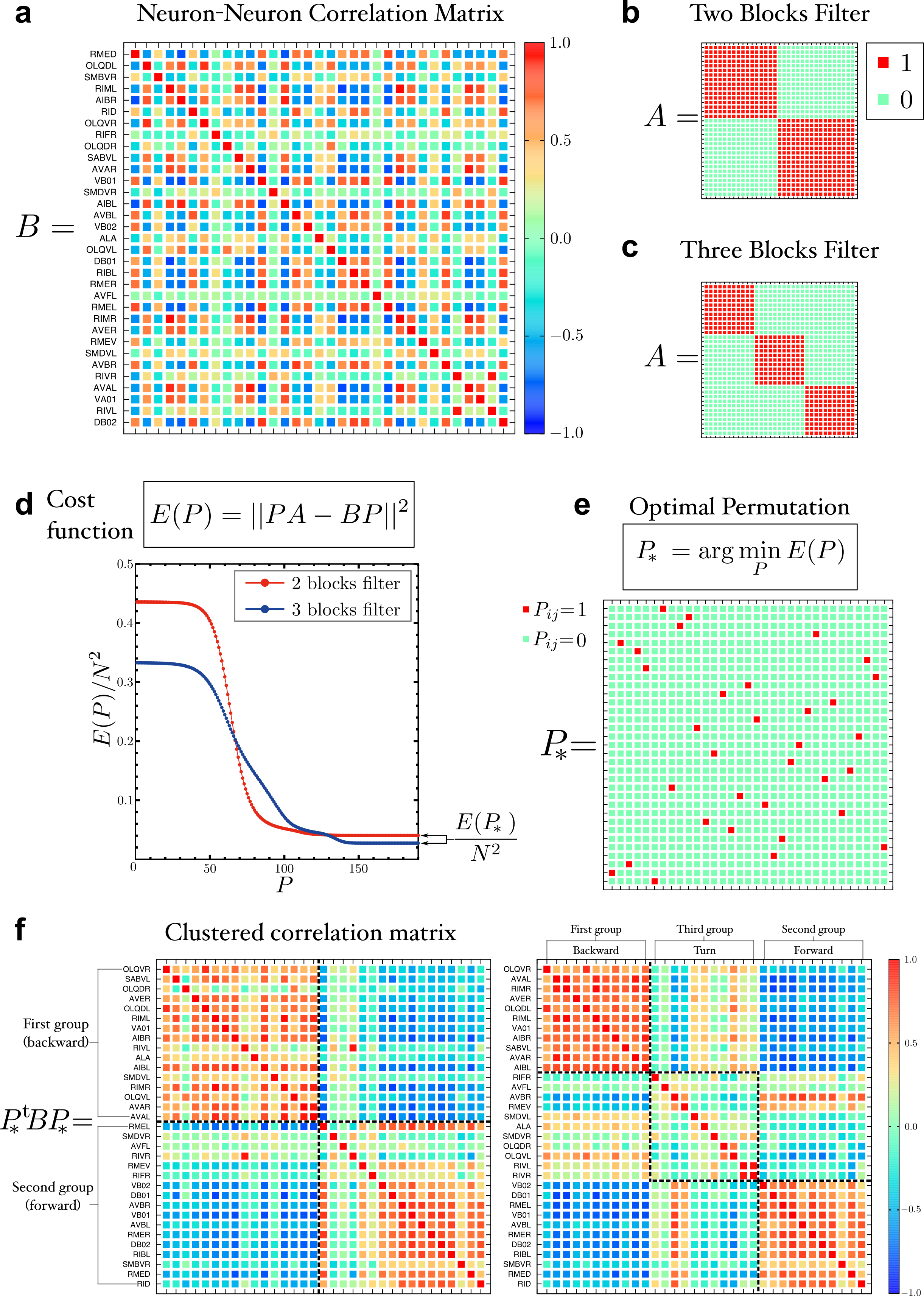
Fig. 1:

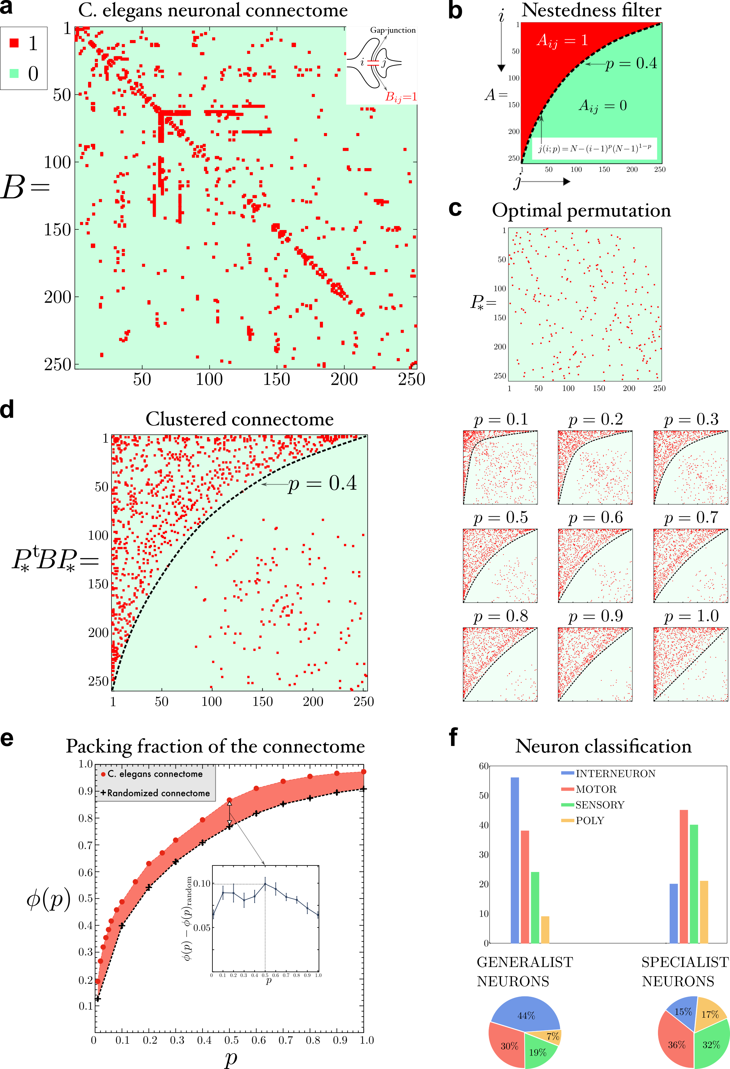
Fig. 2:

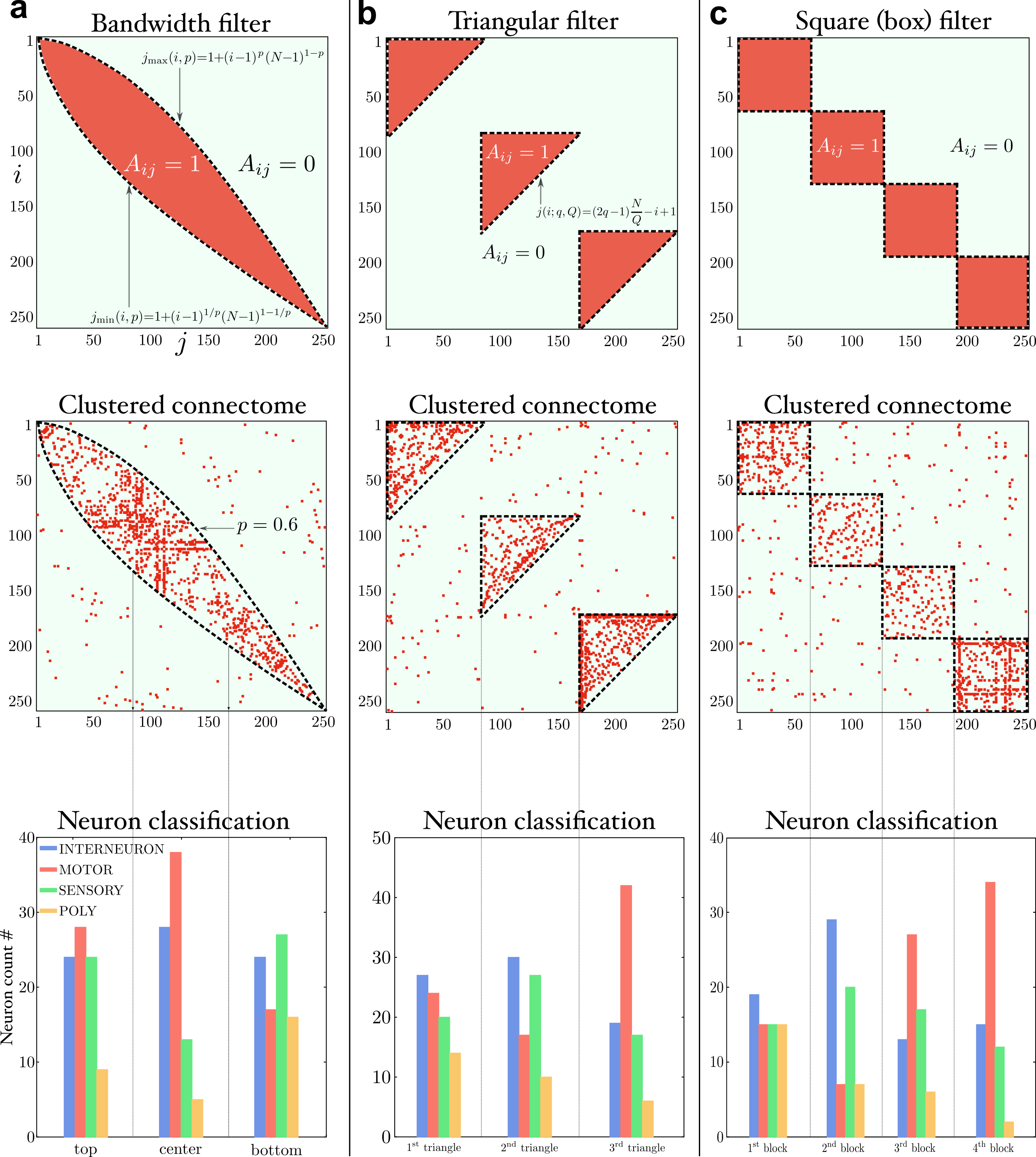
Fig. 3:

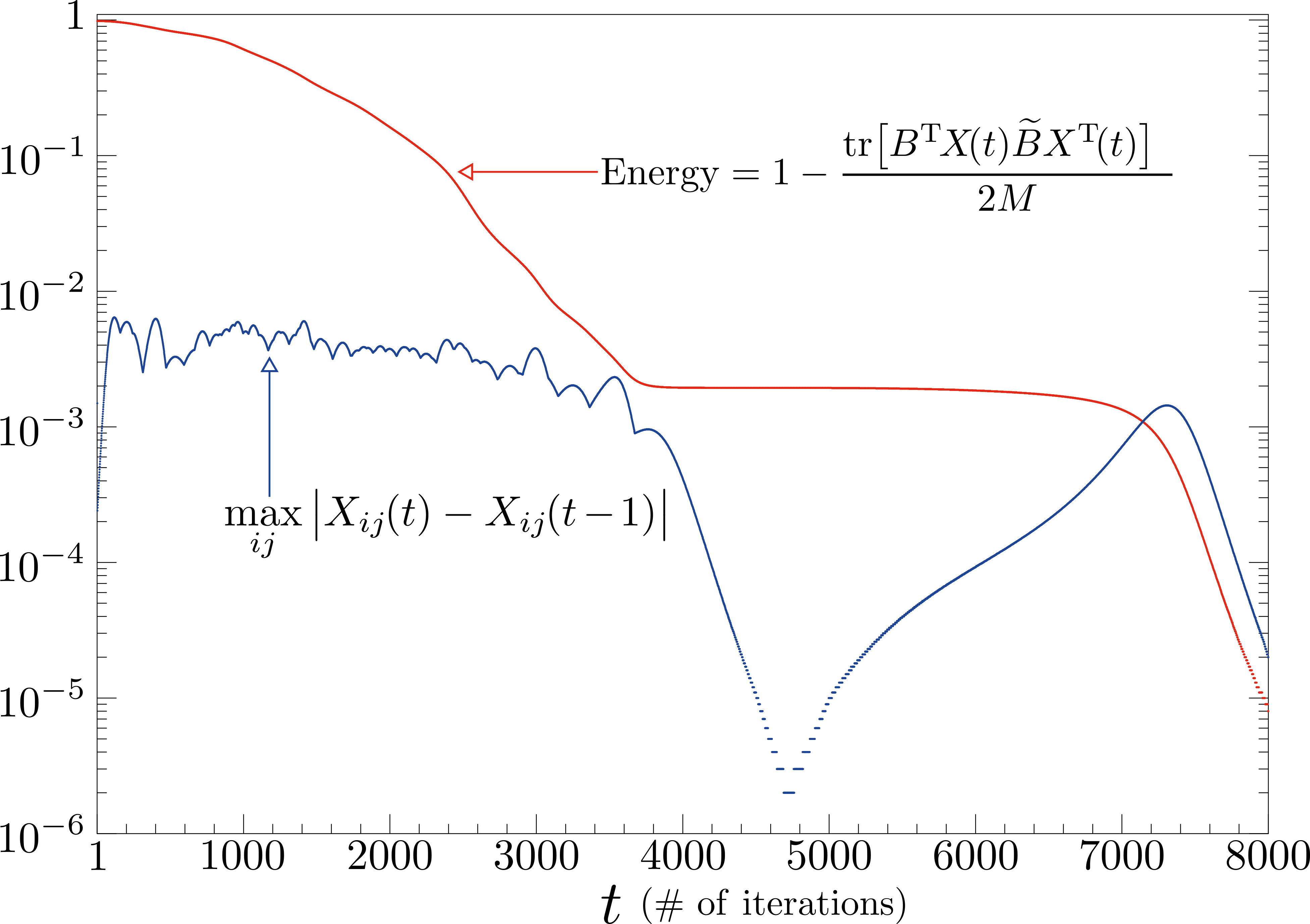
Fig. 4:

Supplementary Information for:

Clustering matrices through optimal permutations

Flaviano Morone

IV The Optimal Permutation Problem (OPP)

We consider two square matrices $A,B\in\mathcal{M}_{N\times N}(\mathbb{R})$, where $\mathcal{M}_{N\times N}(\mathbb{R})$ is the vector space of $N\times N$ real matrices, and the vector space $\mathcal{P}_{N\times N}$ of $N\times N$ permutation matrices $P$ having their entries $P_{ij}\in\{0,1\}$ that satisfy the constraints of row and column sums equal to one: $\sum_{i}P_{ij}=\sum_{j}P_{ij}=1$. Next we define $\Delta(P):\mathcal{P}_{N\times N}\to\mathcal{M}_{N\times N}$ to be the function

$$\Delta(P)=PA-BP\ .$$ (12)

We call $A$ the ‘filter’ (or ‘template’) matrix, and $B$ the ‘input’ matrix. We define the inner product $\langle L|R\rangle$ between two matrices $L,R\in\mathcal{M}_{N\times N}$ by means of the following formula:

$$\langle L|R\rangle={\rm tr}\left(R^{\rm T}L\right)\ ,$$ (13)

where ${\rm tr}$ indicates the trace operation: ${\rm tr}(A)=\sum_{i=1}^{N}A_{ii}$. Then, the norm of $\Delta(P)$ can be computed as:

$$||\Delta(P)||^{2} =\langle\Delta(P)|\Delta(P)\rangle={\rm Tr}\left(A^{\rm T}P^{\rm T}PA-A^{\rm T}P^{\rm T}BP-P^{\rm T}B^{\rm T}PA+P^{\rm T}B^{\rm T}BP\right)=$$ (14)

$$=||A||^{2}+||B||^{2}-2{\rm Tr}\left(B^{\rm T}PAP^{\rm T}\right)=||A||^{2}+||B||^{2}-2{\rm Tr}\left[\left(BPA^{\rm T}\right)^{\rm T}P\right]=$$

$$=||A||^{2}+||B||^{2}-2\langle P|Q(P)\rangle\ ,$$

where we have introduced the ‘overlap’ matrix $Q(P)$, which is defined as follows:

$$Q(P)=BPA^{\rm T}\ .$$ (15)

The quantity we want to optimize over is precisely the inner product $\langle P|Q(P)\rangle$. Therefore, we define the objective (or energy) function $E(P)$ of our problem as

$$E(P)=-\frac{1}{2}\langle P|Q(P)\rangle\ ,$$ (16)

where the factor $1/2$ has been chosen for future convenience. The optimal permutation problem (OPP) is defined as the problem of finding the global minimum (or ground state) of the energy function in Equation (16):

$$\boxed{\ \begin{aligned} {\rm OPP}\ \vcentcolon=\ &{\rm minimize}\ E(P)\\ &{\rm s.\ t.}\ P\in\mathcal{P}\ .\end{aligned}\ }$$ (17)

In order to determine the solution to the OPP given by (17) we take a statistical physics approach by introducing a fundamental quantity called partition function $Z(\beta)$, defined by the following summation:

$$Z(\beta)=\sum_{P\in\mathcal{P}}e^{-\beta E(P)}\ ,$$ (18)

where the notation $\sum_{P\in\mathcal{P}}$ indicates the sum over all $N\times N$ permutation matrices $P$. The parameter $\beta$ in Equation (18) represents, in the statistical physics interpretation of the problem, the inverse of the ‘temperature’ of the system. We notice that the sum in Equation (18) involves $N!$ terms, and thus grows as the factorial of the system size, $Z\sim O(N!)$, rather than displaying the peculiar exponential growth, $Z\sim O(e^{N})$, that appears in the study of the thermodynamic limit of many-body classic and quantum systems.

The global minimum of the objective function in Equation (16) corresponds, physically, to the ‘ground-state’ of the system. But a physical system exists in its ground state only at zero temperature (by the third law of thermodynamics), and thus the exact solution to our optimization (i.e. minimization) problem can be computed by taking the zero temperature limit (which is mathematically tantamount to send $\beta\to\infty$) of the partitition function defined by Equation (18). Specifically, the minimum of $E(P)$ is given by:

$$\min_{P\in\mathcal{P}}E(P)=E(P_{*})=\lim_{\beta\to\infty}-\frac{1}{\beta}\log Z(\beta)\ .$$ (19)

Since the partition function in Equation (18) can be easily calculated when all $P_{ij}$ appear linearly in the argument of the the exponential, a good idea is to write the quadratic term which in the energy connects two variables $P_{ij}$ and $P_{k\ell}$ on different links $i\to j$ and $k\to\ell$ as an integral over disconnected terms. In order to achieve this result, we insert the $\delta$-function

$$\delta(X_{ij}-P_{ij})=\frac{1}{2\pi\imath}\int dJ_{ij}\ {\rm e}^{J_{ij}(P_{ij}-X_{ij})}\ ,$$ (20)

where the integration over $J_{ij}$ runs along the imaginary axis, into the representation of the partition function zinn :

$$Z(\beta)\propto\sum_{P\in\mathcal{P}}\int\prod_{ij}dX_{ij}\int\prod_{ij}J_{ij}\ {\rm e}^{-\beta E(X)\ +\ \sum_{ij}J_{ij}(P_{ij}-X_{ij})}\ ,$$ (21)

To proceed further in the calculation, we enforce the costraint on the column sums:

$$\sum_{i}P_{ij}=\sum_{i}X_{ij}=1\ ,\ \ \ \forall j\ ,$$ (22)

by inserting $N$ $\delta$-functions

$$\delta\Big{(}\sum_{i}X_{ij}-1\Big{)}=\frac{1}{2\pi\imath}\int dz_{j}\ {\rm e}^{-z_{j}\left(\sum_{i}X_{ij}-1\right)}\ ,\ \ \ j=1,\dots,N\ ,$$ (23)

into the partition function:

$$Z(\beta)\propto\sum_{P\in\mathcal{P^{\prime}}}\int\prod_{ij}dX_{ij}\int\prod_{ij}J_{ij}\ \int\prod_{j}z_{j}\ {\rm e}^{-\beta E(X)\ +\ \sum_{ij}J_{ij}(P_{ij}-X_{ij})\ -\ \sum_{j}z_{j}\left(\sum_{i}X_{ij}-1\right)}\ ,$$ (24)

where $\mathcal{P^{\prime}}$ indicates the vector space of $N\times N$ right stochastic matrices $P$ with integer entries $P_{ij}\in\{0,1\}$, that is, matrices with each row summing to one: $\sum_{j=1}^{N}P_{ij}=1$ (but no costraint on the column sums). Then, summation over the variables $P_{ij}$ is straightforward, and we find:

$$\sum_{P\in\mathcal{P^{\prime}}}{\rm e}^{\sum_{ij}J_{ij}P_{ij}}=\prod_{i}\sum_{j}{\rm e}^{J_{ij}}\ .$$ (25)

Introducing the function $F(X,J,z)$ defined by:

$$F(X,J,z;\beta)=E(X)+\frac{1}{\beta}\langle X|J\rangle+\frac{1}{\beta}\sum_{j}z_{j}\Big{(}\sum_{i}X_{ij}-1\Big{)}-\frac{1}{\beta}\sum_{i}\log\sum_{j}{\rm e}^{J_{ij}},$$ (26)

we can write the partition function Equation (24) as

$$Z(\beta)\propto\ \int\prod_{ij}dX_{ij}dJ_{ij}\prod_{j}dz_{j}\ {\rm e}^{-\beta F(X,J,z;\beta)}\ ,$$ (27)

which can be evaluated by the steepest descent method in the limit of zero temperature (i.e. $\beta\to\infty$). The saddle point equations are obtained by differentianting $F$ with respect to $X_{ij}$, $J_{ij}$, and $z_{j}$:

$$\frac{\partial F}{\partial X_{ij}} =-\frac{1}{2}\frac{\partial}{\partial X_{ij}}\Big{[}\sum_{k\ell}X_{k\ell}Q_{k\ell}(X)\Big{]}+\frac{1}{\beta}J_{ij}+\frac{1}{\beta}z_{j}=0\ ,$$ (28)

$$\frac{\partial F}{\partial J_{ij}} =\frac{1}{\beta}X_{ij}-\frac{1}{\beta}\sum_{k}\frac{1}{\sum_{\ell}{\rm e}^{J_{k\ell}}}\sum_{\ell}\frac{\partial}{\partial J_{ij}}{\rm e}^{J_{k\ell}}=0\ ,$$

$$\frac{\partial F}{\partial z_{j}} =\frac{1}{\beta}\Big{(}\sum_{i}X_{ij}-1\Big{)}=0\ .$$

The solution to the saddle point Equations (28) is given by:

$$J_{ij} =\frac{\beta}{2}\left(BXA^{\rm T}+B^{\rm T}XA\right)_{ij}-z_{j}\ ,$$ (29)

$$X_{ij} =\frac{{\rm e}^{J_{ij}}}{\sum_{k}{\rm e}^{J_{ik}}}\ ,$$

$$1 =\sum_{i}X_{ij}\ .$$

Notice that the solution $X_{ij}$ satisfies automatically the condition of having columns summing to one: $\sum_{j}X_{ij}=1$, $\forall i$, as it should. Opposed to this, are the constraints on the row sums, $\sum_{i}X_{ij}=1$ $\forall j$, which are taken into account by the Lagrange multipliers $z_{j}$.

Next, we eliminate $J_{ij}$ in favor of $X_{ij}$ and we make the constraints on the row and column normalizations manifest in the final solution. Introducing the matrix $W(X)$ defined by

$$W_{ij}(X)=\frac{1}{2}\left(BXA^{\rm T}+B^{\rm T}XA\right)_{ij}\ ,$$ (30)

we can write $J_{ij}$ as $J_{ij}=\beta W_{ij}(X)-z_{j}$. Thus, $X_{ij}$ in Equation (29) takes the form

$$X_{ij}=\frac{{\rm e}^{\beta W_{ij}(X)-z_{j}}}{\sum_{k}{\rm e}^{\beta W_{ik}(X)-z_{k}}}\ .$$ (31)

We notice that Equation (31) is invariant under global translations of the form

$$z_{j}\ \to\ z_{j}+\zeta\ ,\ \ \ \forall j\ ,$$ (32)

for arbitary values of $\zeta$. This symmetry is not unexpected and can be traced back to the fact that out of the $2N$ constraints on the row and columns normalization, only $2N-1$ of them are linarly independent, since the sum of all entries must be equal to $N$, i.e., $\sum_{ij}X_{ij}=N$. This translational symmetry can be eliminated, for example, by choosing $\zeta$ in such a way that:

$$\sum_{i}z_{i}=0\ .$$ (33)

In general, the Lagrange multipliers $z_{j}$ in Equation (31) can be eliminated, in principle, by imposing the constraints $\sum_{i}X_{ij}=1$, i.e., by solving th following system of equations:

$$z_{j}=\log\sum_{i}\left(\frac{{\rm e}^{\beta W_{ij}}}{\sum_{k}e^{\beta W_{ik}-z_{k}}}\right)\ ,\ \ \ j=1,\dots,N\ .$$ (34)

We define, just for future notational convenience, the variable $Y_{ij}(X)$ as follows

$$Y_{ij}(X)={\rm e}^{\beta W_{ij}(X)}\ .$$ (35)

Then, we can make the normalization constraints manifest by defining two vectors: a right vector with components $V_{j}$

$$V_{j}={\rm e}^{-z_{j}}\ ,$$ (36)

and a left vector with components $U_{i}$

$$U_{i}=\frac{1}{\sum_{j}Y_{ij}(X)\ V_{j}}\ ,$$ (37)

whereby we can rewrite Equation (31) as

$$\boxed{\ X_{ij}\ =\ U_{i}(X)\ Y_{ij}(X)V_{j}(X)\ }\ ,$$ (38)

where $V_{j}(X)$ can be calculated consistently with $U_{i}(X)$ using the following equations:

$$V_{j}=\frac{1}{\sum_{i}U_{i}\ Y_{ij}(X)}\ .$$ (39)

We notice that Equations (37) and (39) are nothing but the Sinkhorn-Knopp equations sinkhorn1 ; sinkhorn2 to rescale all rows and all columns of a matrix with strictly positive entries (as is indeed each term $Y_{ij}(X)={\rm e}^{\beta W_{ij}(X)}>0$ in the the present case) to sum to one.

V Algorithm to solve the saddle point equations and find the optimal permutation

In order to find the matrix $X_{*}$ that solves equations (28) we set up an algorithm defined by the following iterative procedure. First of all, we need to introduce a regularized kernel $Y(X;\epsilon)$ as follows

$$W_{ij}(X;\epsilon) =W_{ij}(X)+\beta\epsilon X_{ij}\ ,$$ (40)

$$Y_{ij}(X;\epsilon) =Y_{ij}(X){\rm e}^{\beta\epsilon X_{ij}}\ ,$$

with $\epsilon>0$ being a smoothing parameter to be send eventually to zero. In all our experiments we set $\epsilon=10$ at the start, and then decrease it by one, $\epsilon\to\epsilon-1$ until $\epsilon=0$, after each completion of the following routine.

• 1) Initialize $X_{ij}^{(t=0)}\equiv X_{ij}^{(0)}$ at time zero to a uniform matrix as: $X_{ij}^{(0)}=1/N$.

• 2) Calculate the quantity:

  $$Y_{ij}\big{(}X^{(0)};\epsilon;\alpha\big{)}\equiv Y_{ij}^{(0)}=\exp\left[\alpha\beta W_{ij}\big{(}X^{(0)};\epsilon\big{)}+(1-\alpha)\log\big{(}X^{(0)}\big{)}\right]\ .$$ (41)

  We choose $\alpha=10^{-3}$ and $\beta=10$ (the parameter $\alpha$ is a ‘dumping’ factor which helps the convergence of the algorithm).

• 3) Calculate $U_{i}$ and $V_{j}$ as follows:

  • a) Initialize $U_{i}^{(0)}=1$ $\forall\ i$.

  • b) Compute $V_{j}^{(1)}$ and $U_{i}^{(1)}$ using the following equations:

    $$V_{j}^{(1)} =\frac{1}{\sum_{i}U_{i}^{(0)}Y_{ij}^{(0)}}\ ,$$ (42)

    $$U_{i}^{(1)} =\frac{1}{\sum_{j}Y_{ij}^{(0)}V_{j}^{(1)}}\ .$$

  • c) Calculate the quantity $\delta$ defined as follows:

    $$\delta=\max_{i}\left|U_{i}^{(1)}-U_{i}^{(0)}\right|\ .$$ (43)

  • d) If $\delta>10^{-5}$ then start over from step b); otherwise return $U_{i}$ and $V_{j}$.

• 4) Update $X$ by computing $X_{ij}^{(1)}$ as

  $$X_{ij}^{(1)}=U_{i}Y_{ij}^{(0)}V_{j}\ .$$ (44)

• 5) Calculate the quantity $\Delta$ defined by

  $$\Delta=\max_{ij}\left|X_{ij}^{(1)}-X_{ij}^{(0)}\right|\ .$$ (45)

• 6) If $\Delta>10^{-5}$ then start over from step 2); otherwise return $X_{ij}$.

The output matrix $(X_{*})_{ij}$ is not a permutation matrix, but only a double-stochastic matrix, that is a matrix whose entries are real numbers $X_{ij}\in[0,1]$ that satisfies the double normalization condition on row and column sums: $\sum_{i}X_{ij}=\sum_{j}X_{ij}=1$. To find the solution of the OPP we should take the zero temperature limit by sending $\beta\to\infty$: in this limit the solution matrix $X_{*}$ is projected onto one of the $N!$ vertices of the Birkhoff polytope, which represents the optimal permutation matrix $P_{*}$ that solves the OPP. In order to find $P_{*}$ numerically, we use a simple method which consists in finding a solution $X_{*}$ at large, but finite, $\beta$ (we use $\beta=10$), followed by a hard thresholding of the matrix entries $(X_{*})_{ij}$ defined by:

$$(P_{*})_{ij}=\left\{\begin{matrix}1&{\rm if\ }(X_{*})_{ij}\geq 0.99\\ 0&{\rm otherwise}\end{matrix}\right.\ .$$ (46)

VI Filter matrices

Having discussed how to implement the algorithm, we present, next, several types of filter matrices $A$ that we used in our clustering experiments.

VI.1 Nestedness filter

The nestedness filter is described by a matrix $A$ whose nonzero entries $A_{ij}$ are equal to $1$ when the following condition is satisfied:

$$A_{ij}=1\ \ \ {\rm for}\ \ \ 1\leq i\leq N\ \ \ {\rm and}\ \ j\in[1,j_{\rm max}(i,p)]\ ,$$ (47)

where $j_{\rm max}(i,p)$ is given by:

$$j_{\rm max}(i,p)=N-(i-1)^{p}(N-1)^{1-p}\ ,$$ (48)

as shown in Fig. 5a. The parameter $p\in[0,1]$ quantifies the nestedness of the matrix $A$. Specifically, low values of $p$ correspond to a matrix $A$ with a highly nested structure. Opposite to this, large values of $p$, i.e. $p\sim 1$, describe profiles of low nestedness, as depicted in Fig. 5a,c

The density $\rho(p)$ of the filter matrix $A$ defined by Equation (47) is given by

$$\rho(p)=\frac{1}{N^{2}}\sum_{i=1}^{N}\sum_{j=1}^{j_{\rm max}(i,p)}1\ ,$$ (49)

which, in the limit $N\to\infty$, becomes:

$$\boxed{\ \rho(p)=\frac{p}{1+p}\ }\ .$$ (50)

The finite $N$ behavior of $\rho(p)$ together with its $N\to\infty$ limit is showm in Fig. 5b.

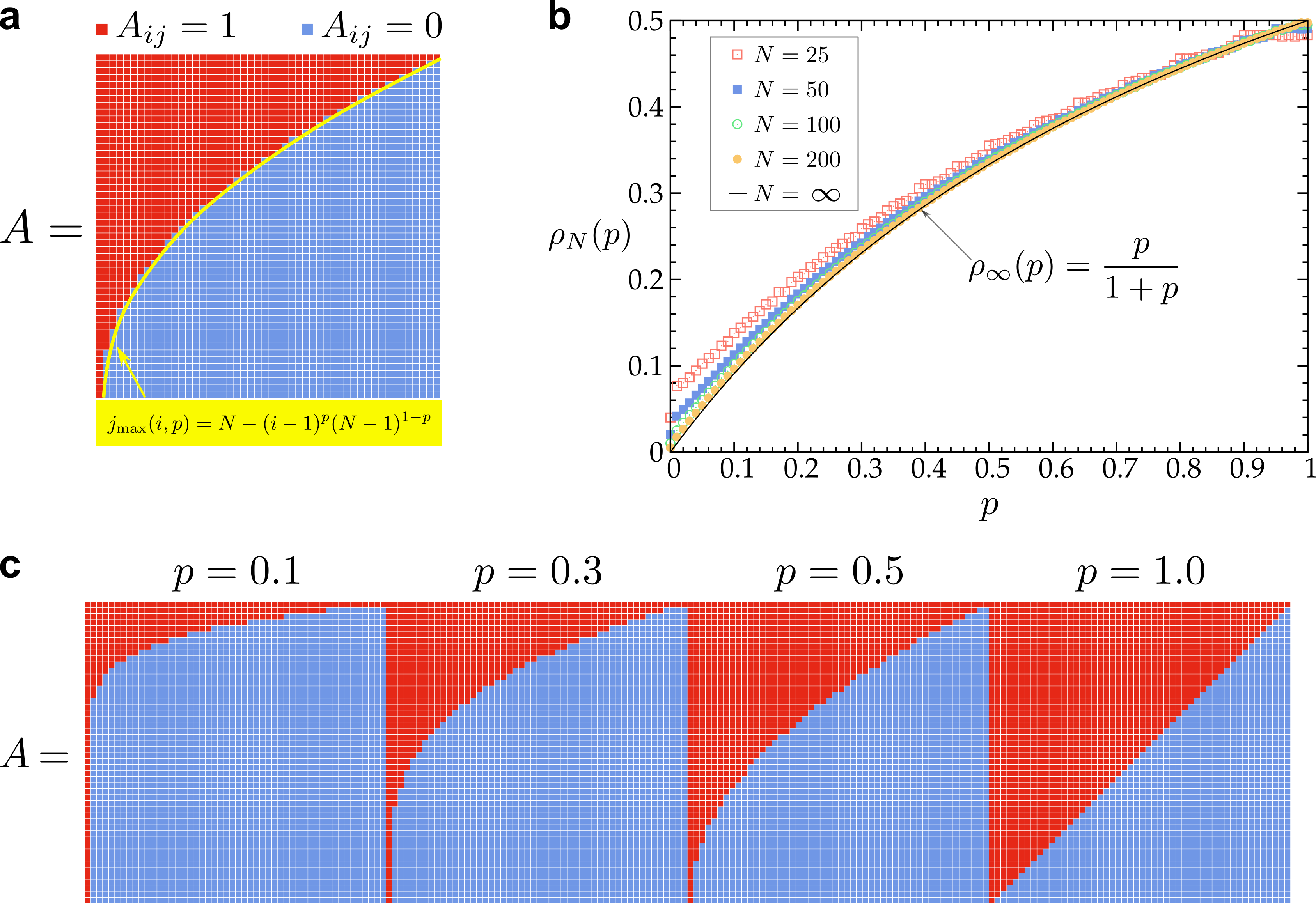
Supplementary Figure 5: Nestedness filter.

VI.2 Band filter

The band filter is a matrix $A$ whose entries $A_{ij}\in\{0,1\}$ are defined by

$$A_{ij}=\left\{\begin{matrix}1&\begin{matrix}{\rm for}\ 1\leq i\leq N\\ j_{\rm min}(i,p)\leq j\leq j_{\rm max}(i,p)\end{matrix}&\\ 0&{\rm otherwise}\end{matrix}\right.\ ,$$ (51)

where

$$j_{\rm min}(i,p) =1+(i-1)^{1/p}(N-1)^{1-1/p}\ ,$$ (52)

$$j_{\rm max}(i,p) =1+(i-1)^{p}(N-1)^{1-p}\ ,$$

where $p$ is a parameter that controls the width of the band, hence we call $p$ the bandwidth exponent. The band filter in Equation (51) has nonzero entries comprised in a band delimited by $j_{\rm min}(i,p)$ and $j_{\rm max}(i,p)$ for $i=1,\dots,N$. The density $\rho(p)$ of $A$ is defined as the fraction of entries contained inside the band:

$$\rho(p)=\frac{1}{N^{2}}\sum_{i=1}^{N}\sum_{j=j_{\rm min}(i,p)}^{j_{\rm max}(i,p)}1\ .$$ (53)

For $N\to\infty$, the density $\rho(p)$ evaluates

$$\boxed{\ \rho(p)=\frac{1-p}{1+p}\ }\ .$$ (54)

The finite $N$ behavior of $\rho(p)$ along with the $N\to\infty$ limit given by Equation (54) are showm in Figure 6b.

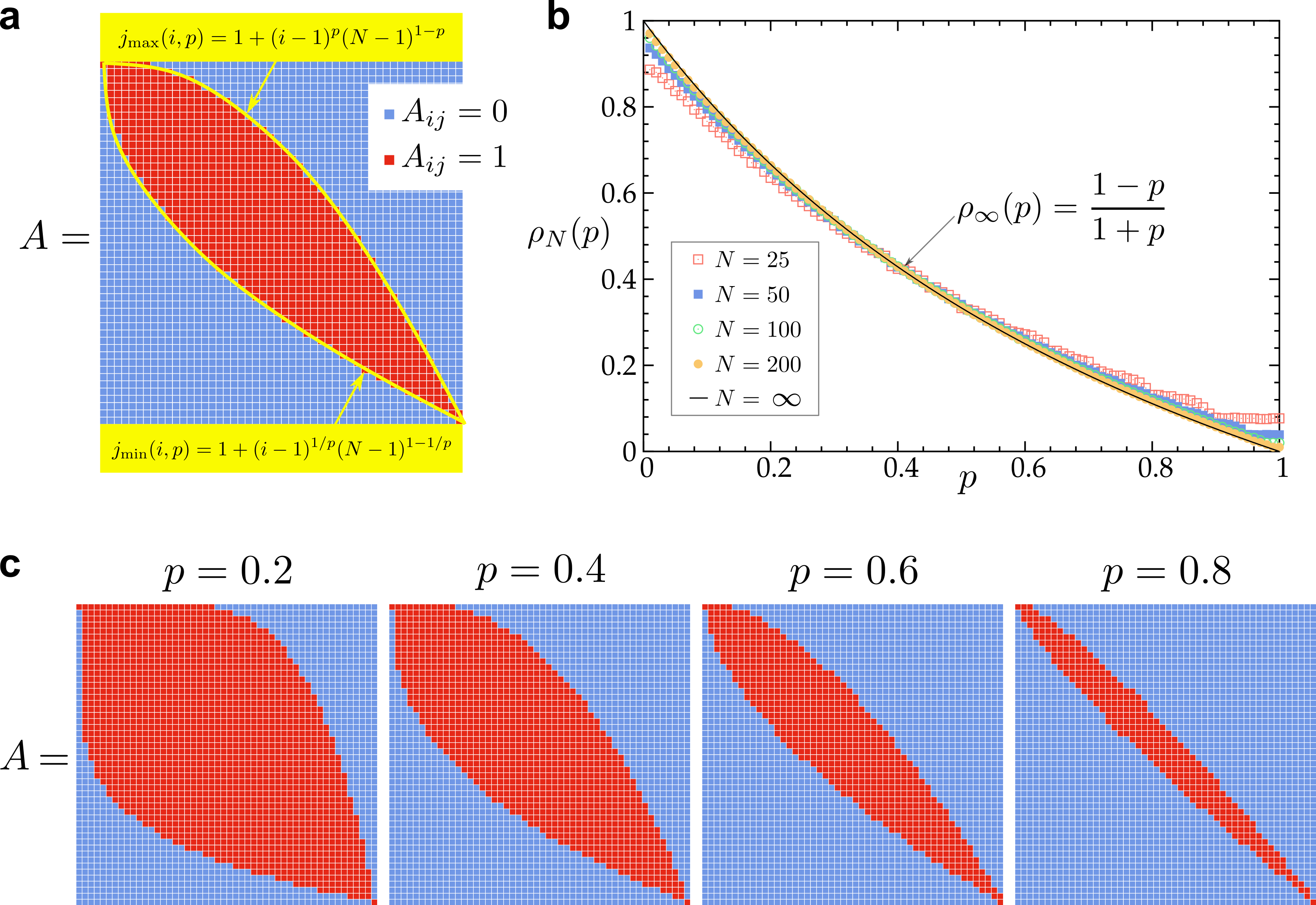
Supplementary Figure 6: Band filter.

A useful quantity to characterize the shape of the band filter is the bandwidth $b(p)$, which is defined by

$$b(p)=\max_{i}[j_{\rm max}(i,p)-j_{\rm min}(i,p)]\ .$$ (55)

Let us define the rescaled coordinate $x$ taking values in the range $x\in[0,1]$ as:

$$x=\frac{i-1}{N-1}\ ,$$ (56)

whereby we can write the difference $j_{\rm max}-j_{\rm min}$ as

$$j_{\rm max}(i,p)-j_{\rm min}(i,p)=(N-1)(x^{p}-x^{1/p})\ .$$ (57)

Next we define the rescaled bandwidth $\widetilde{b}(p)$ as

$$\widetilde{b}(p)=\frac{b(p)}{N-1}\ .$$ (58)

Thus, in the large $N$ limit we can approximate $x$ to a continuous variable and thus estimate $\widetilde{b}(p)$ as follows:

$$\widetilde{b}(p)=x_{*}(p)^{p}-x_{*}(p)^{1/p}\ ,$$ (59)

where $x_{*}(p)$ is the solution to the following equation:

$$\frac{d}{dx}(x^{p}-x^{1/p})\big{|}_{x=x_{*}(p)}=0\ ,$$ (60)

that is:

$$x_{*}(p)=p^{\frac{2p}{1-p^{2}}}\ .$$ (61)

Substituting Equation (61) into Equation (59) we obtain the explicit form of the rescaled bandwidth as a function of $p$

$$\boxed{\ \widetilde{b}(p)=p^{\frac{2p^{2}}{1-p^{2}}}-p^{\frac{2}{1-p^{2}}}\ }\ ,$$ (62)

which is shown in Fig. 7

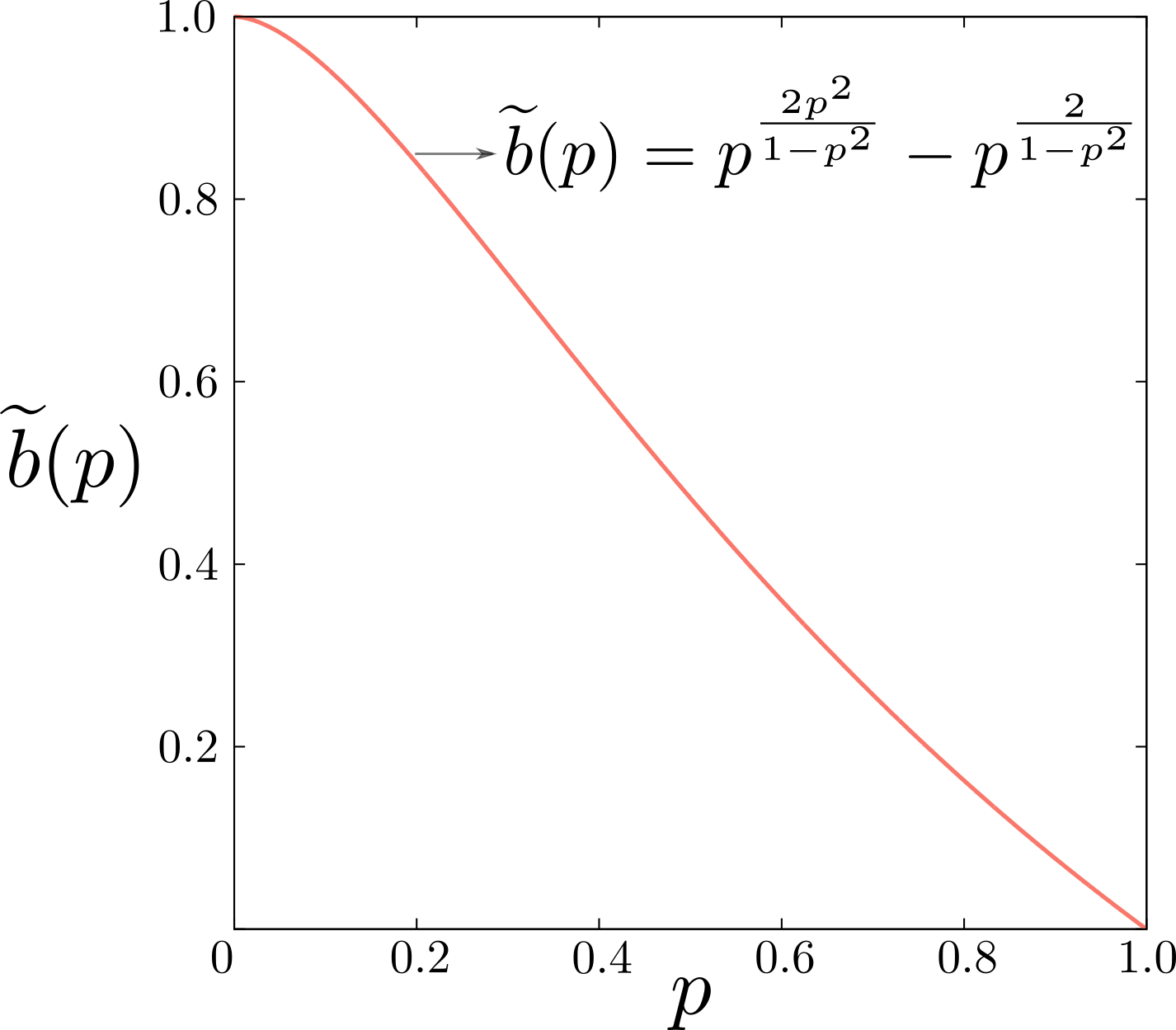
Supplementary Figure 7: Rescaled bandwidth.

VI.3 Square filter and Triangle filter

The square filter $A$ is shown in Figure 8a and is parameterized by a number $Q$ representing the number of blocks the matrix $A$ is divided into. The size of each block is $\frac{N}{Q}\times\frac{N}{Q}$. The $Q$ square blocks are arranged along the main diagonal. Mathematically, the entries $A_{ij}$ of $A$ are defined to be $0$ or $1$ by

$$\begin{aligned} A_{ij}&=1\ \ \ {\rm if}\ \ \ \left\{\begin{matrix}i\in\left[1+(q-1)\frac{N}{Q},q\frac{N}{Q}\right]\\ {\rm AND}\\ j\in\left[1+(q-1)\frac{N}{Q},q\frac{N}{Q}\right]\end{matrix}\ ,\ \ \ q=1,\dots,Q\right.\\ A_{ij}&=0\ \ \ {\rm otherwise}\end{aligned}\ .$$ (63)

The density $\rho(Q)$ is easy to calculate and evaluates:

$$\rho(Q)=\frac{1}{Q}\ .$$ (64)

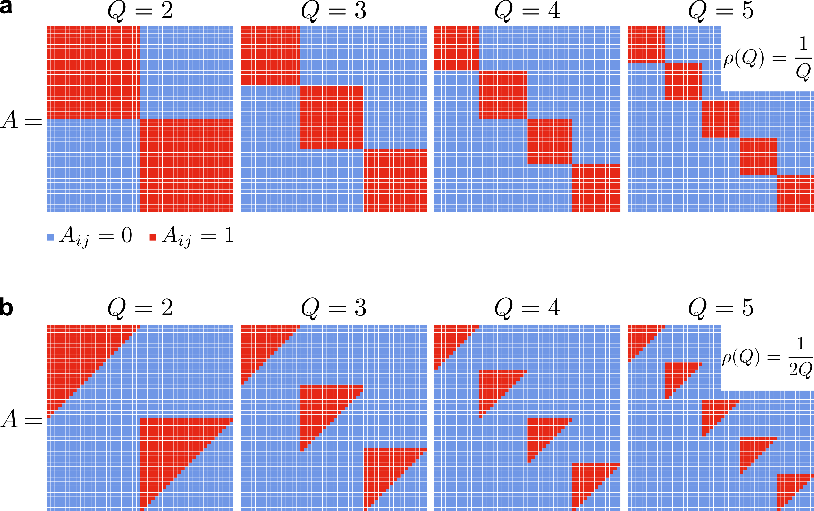
Supplementary Figure 8: Square filter and Triangle filter.

The triangle filter is shown in Figure 8b and is parameterized by a number $Q$ representing the number of equal sized triangular blocks arranged along the main diagonal of the matrix. Mathematically, the entries $A_{ij}$ of $A$ are defined to be $0$ or $1$ by

$$\begin{aligned} A_{ij}&=1\ \ \ {\rm if}\ \ \ \left\{\begin{matrix}i\in\left[1+(q-1)\frac{N}{Q},q\frac{N}{Q}\right]\\ {\rm AND}\\ j\in\left[1+(q-1)\frac{N}{Q},(2q-1)\frac{N}{Q}-i+1\right]\end{matrix}\ ,\ \ \ q=1,\dots,Q\right.\\ A_{ij}&=0\ \ \ {\rm otherwise}\end{aligned}\ .$$ (65)

The density $\rho(Q)$ of the triangle filter equals to

$$\rho(Q)=\frac{1}{2Q}\ .$$ (66)

References

- (1) Golub, G. H. & Van Loan, C. F. Matrix computations edition (Johns Hopkins University Press, 1996).
- (2) D’haeseleer, P. How does gene expression clustering work? Nature Biotechnology 23, 1499–1501 (2005).
- (3) Kato, S., Kaplan, H. S., Schrodel, T., Skora, S., Lindsay, T. H., Yemini, E., Lockery, S. & Zimmer, M. Global brain dynamics embed the motor command sequence of Caenorhabditis elegans. Cell 163, 656-669 (2015).
- (4) Jain, A.K. & Dubes, R. C. Algorithms for Clustering Data (Prentice-Hall, Englewood Cliffs, NJ, 1988).
- (5) Koopmans, T. C & Beckmann, M. Assignment problems and the location of economic activities. Econometrica 25, 53-76 (1957).
- (6) WormAtlas, Altun, Z. F., Herndon, L. A., Wolkow, C. A., Crocker, C., Lints, R. & Hall, D. H. (eds) 2002–2019. https://www.wormatlas.org.
- (7) Zinn-Justin, J. Quantum Field Theory and Critical Phenomena edition (Oxford University Press, 2002).
- (8) Linderman, S., Mena, G., Cooper, H., Paninski & L., Cunningham J. Reparameterizing the Birkhoff Polytope for Variational Permutation Inference. Proceedings of the Twenty-First International Conference on Artificial Intelligence and Statistics 84, 1618-1627 (2018).
- (9) Sinkhorn, R. A relationship between arbitrary positive matrices and doubly stochastic matrices. Ann. Math. Statist. 35, 876–879 (1964).
- (10) Sinkhorn, R & Knopp, P. Concerning nonnegative matrices and doubly stochastic matrices. Pacific J. Math. 21, 343–348 (1967).
- (11) Cuturi, M. Sinkhorn distances: lightspeed computation of optimal transport. Proceedings of the 26th International Conference on Advances in Neural Information Processing Systems, NIPS 26, 2292-2300 (2103).
- (12) Tacchella, A., Cristelli, M., Caldarelli, G., Gabrielli, A. & Pietronero, L. A new metrics for countries’ fitness and products’ complexity. Sci. Rep. 2, 723 (2012).
- (13) Benzi, M., Golub, G. H. & Liesen, J. Numerical solution of saddle point problems. Acta numerica 14 1-137 (2005).
- (14) Varshney, R., Chen, B. L., Paniagua, E., Hall, D. H. & Chklovskii, D. B. Structural properties of the Caenorhabditis elegans neuronal network. PLoS Computational Biology 7(2):e1001066 (2011).
- (15) Patterson, B. D. Atmar, W. Nested subsets and the structure of insular mammalian faunas and archipelagos. Biological Journal of the Linnean Society 28, 65–82 (1986).
- (16) Bascompte, J., Jordano, P., Melián, C. J. & Olesen J. M. The nested assembly of plant–animal mutualistic networks. Proc. Natl. Acad. Sci. 100, 9383–9387 (2003).
- (17) Staniczenko, P. P. A., Kopp, J. C. & Allesina, S. The ghost of nestedness in ecological networks. Nat. Commun. 4, 1931 (2013).
- (18) Konig, M. D., Tessone, C. J. & Zenou, Y. Nestedness in networks: A theoretical model and some applications. Theoretical Economics 9, 695–752 (2014).
- (19) Mariani, M. S., Ren, Z.-M., Bascompte, J. & Tessone, C. J. Nestedness in complex networks: observation, emergence, and implications. Physics Reports 813, 1-90 (2019).
- (20) Kaplan, H. S, Salazar Thula, O., Khoss, N. & Zimmer M. Nested neuronal dynamics orchestrate a behavioral hierarchy across timescales. Neuron 105, 562–576 (2019).
- (21) Morone, F., Del Ferraro, G. & Makse, H. The k-core as a predictor of structural collapse in mutualistic ecosystems. Nat. Phys. 15, 95-102 (2019).
- (22) Newman, M. Networks (Oxford University Press, 2018).
- (23) Chinn, P. Z., Chvátalová, J., Dewdney, A. K. & Gibbs, N. E. The bandwidth problem for graphs and matrices–a survey. J. Graph Th. 6, 223-254 (1982).
- (24) Babai, L. Graph isomorphism in quasipolynomial time. STOC ‘16: Proceedings of the forty-eighth annual ACM symposium on theory of computing, 684–697 (2016).
- (25) Morone, F. & Makse, H. Symmetry group factorization reveals the structure-function relation in the neural connectome of Caenorhabditis elegans. Nat. Commun. 10, 1-13 (2019).