Multi-scale Iterative Residuals for Fast and Scalable Stereo Matching
Abstract.
Despite the remarkable progress of deep learning in stereo matching, there exists a gap in accuracy between real-time models and slower state-of-the-art models which are suitable for practical applications. This paper presents an iterative multi-scale coarse-to-fine refinement (iCFR) framework to bridge this gap by allowing it to adopt any stereo matching network to make it fast, more efficient and scalable while keeping comparable accuracy. To reduce the computational cost of matching, we use multi-scale warped features to estimate disparity residuals and push the disparity search range in the cost volume to a minimum limit. Finally, we apply a refinement network to recover the loss of precision which is inherent in multi-scale approaches. We test our iCFR framework by adopting the matching networks from state-of-the art GANet and AANet. The result is 49 faster inference time compared to GANet-deep and 4 less memory consumption, with comparable error. Our best performing network, which we call FRSNet is scalable even up to an input resolution of 6K on a GTX 1080Ti, with inference time still below one second and comparable accuracy to AANet+. It out-performs all real-time stereo methods and achieves competitive accuracy on the KITTI benchmark.
1. Introduction
Stereo matching is one of the top research areas in modern computer vision, with enormous applications in the industry particularly in autonomous driving and robotics. The idea is to reconstruct dense 3D geometry by estimating the disparity between image pixels in a rectified stereo image pair. To this end, dense matching pixel correspondences are used. Since, this is one of the major classical problems in computer vision, it has been studied substantially for more than half a century (Zhang and Liu, 2014) and has been matured. A huge amount of literature is available proposing various architectures both classical and modern, which aim to solve the problem of stereo matching successfully. A large part of these are deep neural networks. Although most of these networks provide sub-pixel accuracy with a state-of-the-art pixel outlier rate, a small number of them concentrate on the execution time and model growth, especially in the case of end-to-end trainable networks. The architectures with a design focus on run-time have much worse end point errors (EPE) and pixel error rates (ER) and are not comparable to the state-of-the-art models at all (Khamis et al., 2018; Duggal et al., 2019; Zhang et al., 2019).
The problem of stereo matching is solved traditionally with some key steps namely: 1) Extracting features, 2) Cost volume construction, 3) Cost aggregation for matching, 4) Regressing the final disparity. Two types of approaches exist in the literature incorporating some or all of these steps. These are direct disparity regression without building a cost volume and by using cost volume filtering. The first category disregards geometric variations by calculating disparity on dense matching pixel correspondences. These approaches although being relatively fast lead to large EPE and ER (Hirschmuller, 2005). The latter namely volumetric methods, construct and refine a cost volume. The idea is to build a higher dimensional feature volume containing all the candidate disparity values up to a maximum disparity range. These approaches are slower in classical processing as they incorporate some customized versions of dynamic programming algorithms for finding the best matching features over the cost volume. Neural networks built on volumetric matching often use two sub-networks in an end-to-end architecture. The first sub-net extracts features from the stereo image pairs which are used to build a 3D or 4D cost volume. The second network then uses 3D convolutions to compute matching costs in the cost volume before finally regressing the final disparity values. The run-time for these models is also nowhere comparable to real-time as these have to employ heavy operations on the high dimensional cost volume.
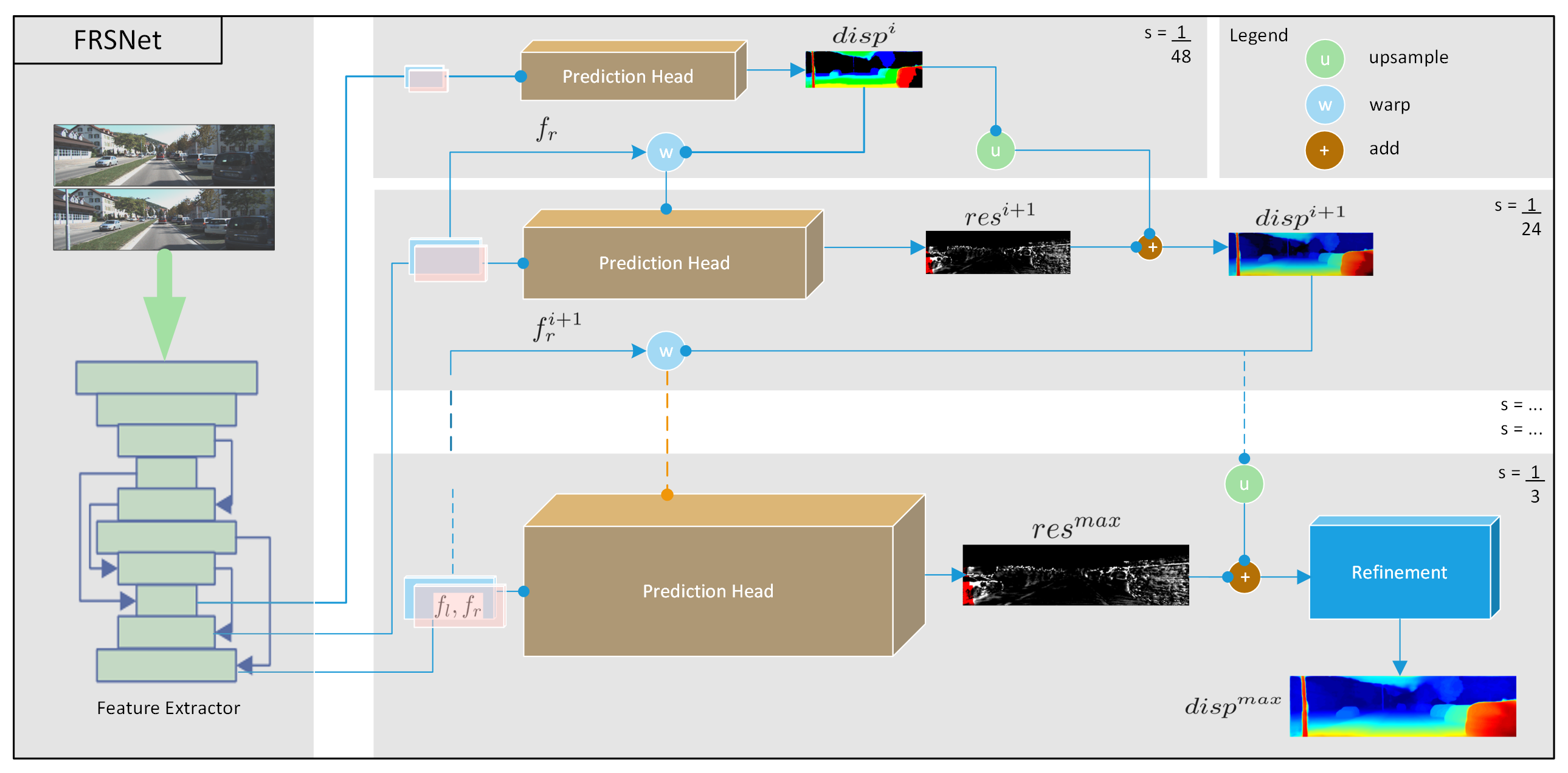
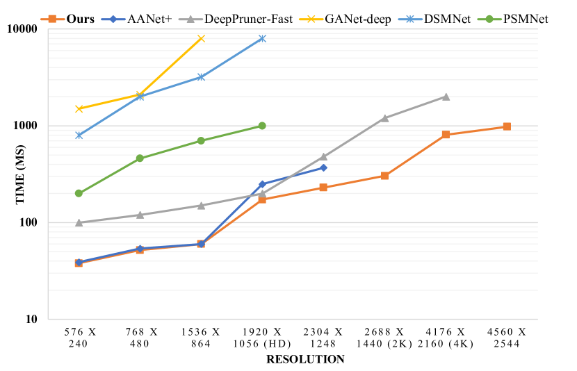
There exists a gap in the literature between real-time models with higher EPE and ER and slower state-of-the-art models with lower EPE and ER. We aim to bridge this gap by proposing a novel multi-scale coarse-to-fine refinement framework to estimate disparity by leveraging the already produced features usually at different resolutions by the feature extraction backbone and using much shallower cost volumes. These lower resolution disparity maps are then iteratively refined using the notion of disparity residuals. The idea being that these lower resolution operations on smaller disparity search ranges will be computationally more efficient and much more scalable in terms of memory while keeping the EPE and ER comparable. As shown in Figure 6 and Table 2, our approach bridges the accuracy gap between the real-time and state-of-the-art stereo matching models such as GANet (Zhang et al., 2019) and AANet (Xu and Zhang, 2020), while staying as close as possible to real-time performance.
We introduce the notion of a prediction head, which can be adopted from any stereo matching architecture and is used in our iterative coarse-to-fine refinement algorithm (iCFR). Separate heads are produced for each scale and their parameters are learned in an end-to-end fashion. We also propose a final refinement layer to recover the loss of precision that is inherent in down and upsampling operations. The resulting final network which we call FRSNet (Fast iterative Residual Stereo Network), using the iCFR, outperforms all available real-time architectures for stereo matching such as StereoNet (Khamis et al., 2018), DispNet (Mayer et al., 2016), Toast (Zbontar and LeCun, 2015a) and other deeper networks like GC-Net (Kendall et al., 2017a) while producing comparable EPE and ER to modern state-of-the-art networks such as AANet (Xu and Zhang, 2020), PSMNet (Chang and Chen, 2018) and GANet (Zhang et al., 2019), on the Sceneflow dataset (Mayer et al., 2016) and the KITTI benchmark (Geiger et al., 2012).
2. Related Work
Traditional algorithms for stereo matching (Hirschmuller, 2005; Falkenhagen, 1997; Schonberger et al., 2018; Yang, 2012; Min et al., 2011) yield discontinuous disparity maps with higher pixel outlier rates. This is because they usually use feature-based matching which does not take the geometric variations in images into account. Thus, the matching is ambiguous, due to occlusions, reflections, texture-less surfaces and repetitive patterns. Volumetric methods with cost volume construction and cost aggregation strategies were developed to achieve better matching (Yang, 2012; Jancosek and Pajdla, 2009; Liu et al., 2009). Then with the advent of deep learning, these strategies transformed into learnable layers in terms of convolution and other operations. The first deep learning architecture for stereo matching was proposed in MC-CNN (Zbontar and LeCun, 2015b), which used a feature extraction network instead of handcrafted features. Then, DispNet (Mayer et al., 2016) provided a real-time end-to-end disparity estimation approach by using an encoder-decoder to directly regress the final disparity map. Since this network does not use prior information, it is completely data-driven and requires a huge dataset to train on. To this end, the authors of DispNet also presented the synthetic Sceneflow dataset (Mayer et al., 2016) to train such kind of end-to-end networks, which we also partially use to train our network. Then a two-stage convolutional neural network was presented by Pang et al. (Pang et al., 2017), which separates the workflow for feature extraction and disparity refinement. The first approach with a 4D cost volume was proposed in GC-Net (Kendall et al., 2017a). It applies 3D convolutions to aggregate the matching costs. GC-Net presents a three stage end-to-end trainable network for stereo estimation following the key steps of stereo matching i.e. feature extraction, cost aggregation and disparity regression. It achieved state-of-the-art accuracy, however the inference times are much higher compared to the real-time models.
PSMNet (Chang and Chen, 2018) uses a feature pyramid network and stacked hourglass network along with twenty-five convolution layers to achieve state-of-the-art EPE and ER. However, higher number of convolutional layers deteriorate the run-time quite considerably and puts it far from the real-time category. GANet (Zhang et al., 2019) proposes to incorporate geometric optimization algorithms like SGM (Hirschmuller, 2005) in deep learning pipelines as learnable layers. To this end, it presents the concept of guided aggregation layers in the end-to-end pipeline. These layers aim to leverage the local neighbourhood information as well as the global image context into guiding convolutions in the cost aggregation network. These layers push the sub-pixel accuracy even further and replace a large number of computationally complex 3D convolutions. LEAStereo (Cheng et al., 2020) applies neural architecture search to choose the best possible parameters for a set of operations performed in the network for stereo matching. It achieves state-of-the-art accuracy on KITTI benchmark as well as close to real-time performance. This however, requires enormous amounts of computational resources to compute the best neural architecture for the job. To cater for this, the authors applied task-specific human knowledge to come up with a three step stereo matching architecture and refined the parameters with the neural architecture search, e.g. convolution filters sizes, strides, etc. Other faster techniques use coarse-to-fine matching with hierarchical upsampling (Tankovich et al., 2021; Yin et al., 2019; Duggal et al., 2019; Chen et al., 2019; Yu and Gao, 2020; Gu et al., 2020). Among them, DeepPruner achieves great performance. However, they ignore recovering details lost by lower resolution matching. Despite considerable research for the last half-century, a stereo matching architecture with a focus on practical implications is still an open question in the computer vision community, where a state-of-the-art algorithm can be applied to real-time applications. Our approach takes a step in this direction.
3. FRSNet: A Multi-scale Improvement
In this section, we describe the details of our proposed multi-scale iterative coarse-to-fine refinement framework for stereo matching (iCFR) and a proposed best performing network called FRSNet which uses this iCFR. The overall architecture is shown in Figure 1.
3.1. Feature Extraction
As a feature extraction backbone, we employ a stacked hourglass network with skip connections between corresponding layers of the encoder and decoder (Zhang et al., 2019; Xu and Zhang, 2020). This densely connected network is shared by the input stereo image pair. We use the already calculated features at multiple scales from the decoder part (i.e. ), as input to the prediction heads at the corresponding scales. Figure 1 shows the feature extraction network with dense connections. These features are then either concatenated or correlated to form the cost volume which is then processed in the prediction head.
3.2. Prediction Head
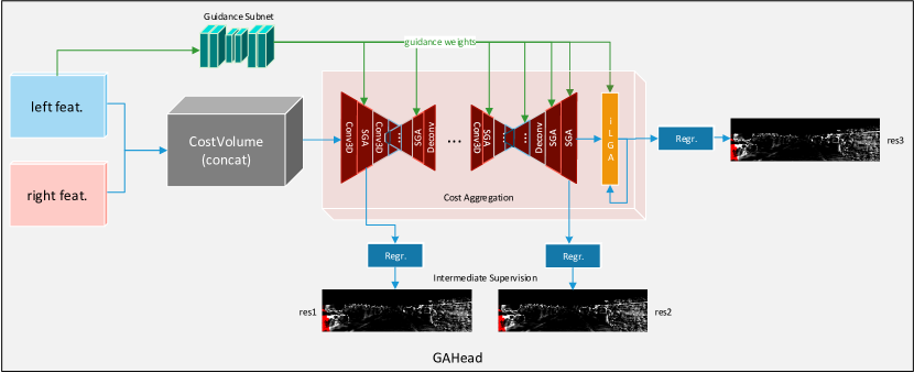
We combine the three latter parts of the stereo matching pipeline namely cost volume construction, cost aggregation and disparity regression into a prediction head, for modularity. Modern volumetric end-to-end stereo matching architectures such as GC-Net (Kendall et al., 2017a) and GANet (Zhang et al., 2019) employ a 4D cost volume. This cost volume is built by either concatenating or correlating the features from the stereo image pair, extracted from the feature extraction backbone, typically a stacked hourglass network (Newell et al., 2016) or a Feature Pyramid (Lin et al., 2017). Depending on the adaptation from any stereo matching network, the cost volume can have different dimensions. Typically a correlation cost volume requires much less memory and a lower number of learnable parameters. The cost volume is then filtered by the adapted strategy of the corresponding stereo matching architecture. Finally, the disparity regression layer estimates the output disparity map. Note that the prediction head is designed to be adopted from any stereo matching architecture. As shown in Figure 3, the prediction head can also produce multiple disparity maps from different stages of cost aggregation for intermediate supervision during training. The ground truth is down-sampled accordingly to calculate the loss for each of these predictions. Sections 3.6 and 3.7 describe the working of the overall multi-scale architecture using prediction heads from two state-of-the-art networks GANet (Zhang et al., 2019) and AANet (Xu and Zhang, 2020).
3.2.1. Symmetric Cost Volume
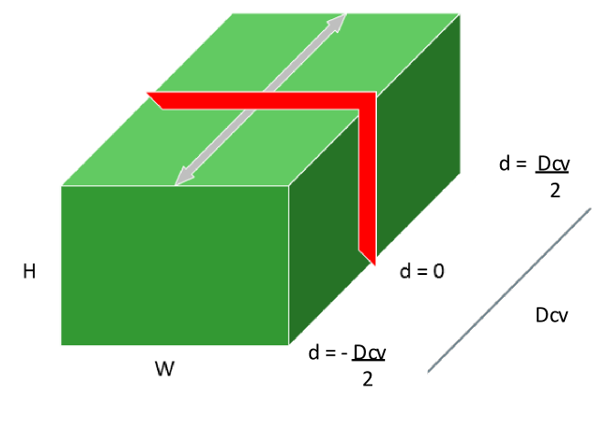
The disparity map produced at the smallest scale i.e. is a very coarse estimate, usually consisting of just blobs of information. These blobs when up-sampled, produce large erroneous estimates of disparity initially. If these are not corrected in the next subsequent scale, the error keeps accumulating and amplifying much like a drift error. Negative disparity residuals are required to correct such coarse estimates. These residuals will help reduce the disparity values if they are initially too high. To this end, we change the way the cost volume is build to allow negative disparity hypotheses. Figure 2 illustrates the construction of such a cost volume. The shape of the cost volume will remain the same , however the way it is filled along the disparity dimension, will be different. The idea is to fill the disparity dimension of length , with disparity hypotheses symmetrically in both directions, i.e. positive and negative. This means that in position , the candidate with zero displacement will be placed. From here in both directions, the cost volume will be filled for the range respectively, leaving out one disparity candidate at the negative search space if required due to rounding. It is worth noting here that after this change the effective search space for disparity is .
3.2.2. Disparity Regression
For calculating the final disparity map we use disparity regression as proposed by Kendall et al. (Kendall et al., 2017b). This yields a much more continuous and consistent disparity map than just using classification based operations. The disparity prediction is given by:
| (1) |
Pseudo-probabilities for each disparity candidate are calculated from the filtered cost volume by applying the softmax operation . Note that the summation bounds in the equation above are consistent with the cost volume construction for negative disparity candidates.
3.3. iCFR: Iterative Coarse-to-Fine Refinement
As shown in Figure 1, the overall network architecture works in a coarse-to-fine refinement fashion using features at multiple scales from the feature extractor. The initial coarse disparity map is calculated at of the original resolution, with the prediction head for the corresponding scale. This is then up-sampled to the next finer scale i.e. . Then the right image features at th scale () are warped towards this up-sampled . The idea is that these warped features will only represent the remaining disparity to be calculated. These are then passed to the prediction head for scale. Since the target image features are now warped, the prediction head will only produce a residual of the full disparity map . Finally the up-sampled coarse disparity map at is added to this residual map to get a refined disparity map at this scale, i.e. . This process is iterated for all scales i.e. {} to get the fine grained disparity map at resolution. The is then passed through the refinement network to get a final refined disparity map at input resolution. A simplified pseudo-code of the iCFR is shown in Algorithm 1. Although the iterations at multiple resolutions introduce additional computational effort for calculating the final refined disparity, these computations follow a geometric series applying the sub-sampling factor (usually 2). This means the computational cost can only be twice w.r.t. the highest resolution for infinitely many sub-scales of iCFR. This is worth investing, considering the saved computations due to the smaller cost volumes at every scale.
3.3.1. Disparity Search Range:
Due to the use of prediction heads at different scales and because each subsequent disparity map is up-sampled for the next scale, the disparity values are also scaled appropriately. This means the for the cost volume can be considerably reduced leading to a much shallower cost volume. For example a of 12 at scale is scaled to 96 at the scale . The can be chosen so that at the highest scale, this value can estimate a of typically 192 pixels, which is usually seen in the state-of-the-art models. For any prediction head, the number of scales and the is to be chosen correctly. The is given by:
| (2) |
where {} in the presented case. The drastic effect of reduction in on inference time is shown in Table 2.
3.4. Refinement Network
As discussed in Section 3.3, the is produced at scale . It typically has some edge gradient effects due to the multi-scale approach. These effects are especially visible on object boundaries and on areas where there is occlusion. To get rid of these artefacts, a final refinement block is applied. We use a stacked hourglass refinement layer as proposed by AANet+ (Xu and Zhang, 2020). We calculate the photometric consistency error (Chabra et al., 2019) and use that as an additional input to the refinement network, along with the left and right images. The refinement network then hierarchically up-samples the prediction at to input resolution and produces geometrically consistent and continuous disparity maps covering thin areas.
3.5. Loss Function
The loss function that is typically used with the disparity regression layer is smooth loss which we adopt in our pipeline too. This is because smooth loss is quite robust against outliers and noise, and therefore helps against disparity discontinuities. We define our loss as:
| (3) |
| (4) |
Here, is the absolute error in the predicted disparities and is the number of ground truth label pixels. The final loss function is the weighted sum of losses over all predictions:
| (5) |
where is a scalar weight and is the total number of predictions for intermediate supervision.

3.6. GAHead
We apply the iCFR algorithm as described in Section 3.3 on state-of-the-art GANet (Zhang et al., 2019) to significantly reduce its memory footprint and inference time. To this end we replace the prediction head in our network with the GANet matching network i.e. the prediction head now consists of concatenation based 4D symmetric cost-volume, guidance subnet, cost aggregation network (SGA and LGA layers) and disparity regression network. We call it GAHead and it is visualized in Figure 3(a). The guidance weights are calculated by the multi-scale guidance subnet on top of the feature extraction network which are reshaped and normalized for use in cost aggregation.
| with GAHead | ||||
| Sym-CV | Improvements | HG-Ref | EPE [px] | ER [%] |
| - | - | - | 7.06 | 51.9 |
| ✓ | - | - | 3.34 | 22.1 |
| ✓ | ✓ | - | 1.01 | 18.2 |
| ✓ | ✓ | ✓ | 0.93 | 17.5 |
| with AAHead | |||
| Sym-CV | HG-Ref | EPE (px) | ER (%) |
| - | - | 4.91 | 43.1 |
| ✓ | - | 2.08 | 23.2 |
| ✓ | ✓ | 0.98 | 16.9 |
3.6.1. Improvements to the GAHead
To push the GAHead performance even further we propose some improvements. Firstly, we replace a 3D convolution layer with an additional SGA layer, with additional guidance weights. This is because SGA layers are much faster than convolution layers and capture the disparity directly (Zhang et al., 2019; Hirschmuller, 2005). Secondly, several LGA layers can be applied before and after passing it to the disparity regression layer to refine smaller details and fine structures in the final disparity map. However, instead of using multiple local guidance weights for each layer, we propose cost filtering using the same weights multiple times i.e. in an iterative manner. This is inspired by the idea of CSPN (Cheng et al., 2019). The filters are shared between iterations, thus keeping the number of learnable parameters constant. With each iteration, more details of the image are revealed which in turn improve the per-pixel depth estimation results. The number of iterations is experimentally determined with the best EPE obtained for , without introducing too much overhead in run-time.
3.7. AAHead
We also apply the iCFR algorithm on state-of-the-art AANet (Xu and Zhang, 2020) to reduce FLOPs and increase its scalability. To this end, we replace the prediction head with the adaptive aggregation module as described in AANet (Xu and Zhang, 2020), which consists of intra/cross-scale aggregation operations. So the prediction head (AAHead, see Figure 3(b)), now consists of a correlation-based 3D symmetric cost volume, an adaptive aggregation network and disparity regression. Since the AAHead works with feature pyramids, for each scale of the iCFR algorithm a nested feature pyramid at {} sub-resolutions is constructed. The coarsest scale is omitted in this case because of the bottleneck in the adaptive aggregation module. To compensate for this reduction, the is set to 24 according to Eq. 2 to keep the close to 192. The adaptive aggregation network employs several modulated deformable convolution layers to aggregate the cost at different scales which has a higher receptive field than normal convolution operation (Zhu et al., 2019). Reduction in FLOPs due to lower resolutions and a much shallower cost volume results in a scalable and much more efficient overall model with even better sub-pixel accuracy and pixel outlier rate than the original AANet as shown in Table 2.
| Method | Resolution | Params | Mem | FLOPS | EPE [px] | D1 [%] | Time [ms] | ||
| GANet (Zhang et al., 2019) | KITTI | 48 | 192 | 6.5M | 6.2G | 2.2T | 0.54 | 1.80 | 7402 |
| FRSNet-GA | KITTI | 4 | 186 | 6.5M | 1.4G | 373G | 0.74 | 2.80 | 150 |
| HD | 4 | 186 | 6.5M | 5.7G | 718G | - | - | 452 | |
| 4K | 4 | 186 | 6.5M | 10G | 1.14T | - | - | 991 | |
| AANet (Xu and Zhang, 2020) | KITTI | 64 | 192 | 8.4M | 4.4G | 575G | 0.55 | 2.03 | 62 |
| HD | 64 | 192 | 8.4M | 7.8G | 793G | - | - | 191 | |
| FRSNet-AA | KITTI | 8 | 180 | 3.1M | 1.4G | 245G | 0.50 | 1.40 | 61 |
| HD | 8 | 180 | 3.1M | 3.8G | 457G | - | - | 173 | |
| 4K | 8 | 180 | 3.1M | 9.9G | 981G | - | - | 692 |
4. Experiments
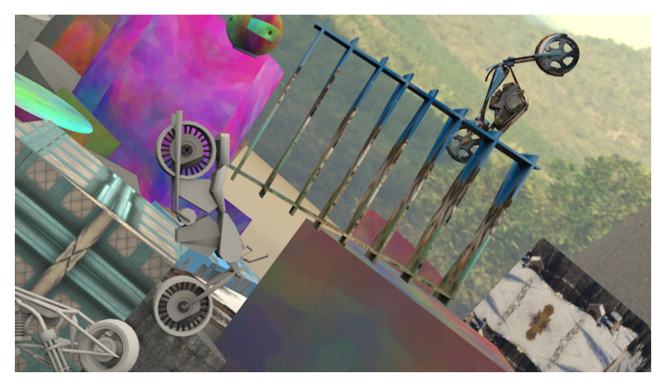
We perform exhaustive experiments on our FRSNet using the Sceneflow and KITTI 2015 datasets. The first proposed by Mayer et al. (Mayer et al., 2016), is a large dataset of synthetic images with dense ground truth. The KITTI dataset (Geiger et al., 2012) contains real-world outdoor images but with sparse ground truth. We report end-point-error (EPE) and 1-pixel outlier rate (ER) on the Sceneflow dataset and EPE and D1 rate on KITTI datasets. The network is implemented in PyTorch. Our final model uses Adam () as optimizer. We employ a three-stage training strategy for all our experiments. 1) Training on Sceneflow dataset, 2) Fine-tuning on KITTI dataset, 3) Optionally, fine-tuning on the (dense) pseudo-ground truth as proposed in AANet (Xu and Zhang, 2020). This third step is required to produce visually consistent disparity maps for upper regions of KITTI images where there is no ground truth disparity available (c.f. Figure 4). We set the value to 12 and 24 for experiments with GAHead and AAHead, respectively. Training is done for 30 epochs with a batch size of 32 on two NVIDIA V100 32GB GPUs, with the crop-size of on Sceneflow dataset and for 1000 epochs with a batch size of 16 on the KITTI datasets with the crop size of . The third fine-tuning stage is carried out for a maximum of 8 epochs. The learning rate begins at 0.001 with a schedule for halving at 400th, 600th and 800th epoch in the fine-tuning phase. All the input image channels are normalized by subtracting their means and dividing their standard deviations. The loss weights in Eq. 5 for multiple predictions are set to [] for the three (two intermediate + final) predictions of the finest pyramid scale and the ultimate prediction at input resolution of the refinement network, in this order.


4.1. Ablation Study
To validate the performance of the proposed iCFR algorithm on the proposed FRSNet, we perform several experiments on the Sceneflow test set and on our KITTI validation set of 15 image pairs, which are obtained by splitting the training set for KITTI 2015 dataset randomly. The ablation experiments involve using the GAHead and AAHead in FRSNet and evaluating the effectiveness of different improvements proposed in Section 3. Table 1 shows the overall results of the ablation study for both predictions heads on the Sceneflow test set. In both cases, it highlights the importance of having a symmetric cost volume (Sym-CV) with negative disparity hypotheses which decreases the EPE and ER by almost half. With GAHead, the introduction of the proposed improvements lower the error metrics even further. It was noted that replacing a higher resolution 3D convolution layer in cost aggregation with a SGA layer not only reduces the EPE and ER but also reduces the inference time by 70 ms.
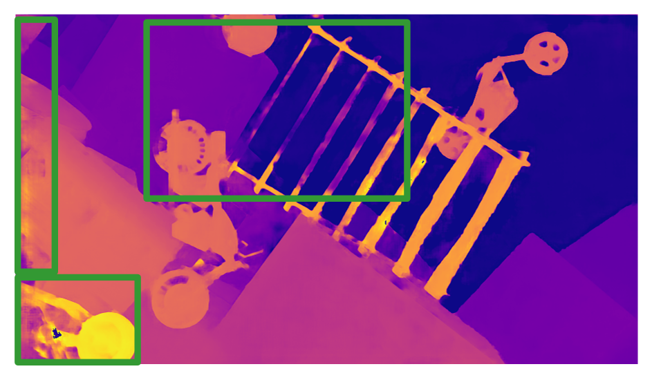
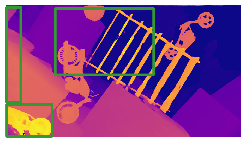
Using the AAHead, without the final refinement layer yields relatively worse predictions than with GAHead. However, with a final hourglass refinement block (HG-Ref) as proposed in AANet+ (Xu and Zhang, 2020) both variants of our model reach sub-pixel accuracy in EPE with the best ER. Similar improvements are seen while evaluating on the KITTI 2015 validation dataset. The positive impact of the refinement block is illustrated in Figure 5. A quantitative evaluation is given in Table 3 in which the hourglass refinement block (HG-Ref) is also compared against an alternative refinement module of SDRNet (Chabra et al., 2019).


4.2. Performance Comparison
Table 2 shows a comprehensive comparison between our network with GAHead and AAHead and the corresponding original networks on our KITTI 2015 validation set. There is a significant decrease in the number of parameters, memory consumption, FLOPs and inference time. Our model only requires 16% of the FLOPs required for the GANet-deep (Zhang et al., 2019), while consuming 6 less memory. Similar improvement is seen compared to AANet (Xu and Zhang, 2020) where the memory requirement is less than half while D1 being 31% better, with a comparable run-time. As also shown in Figure 6, our model can scale up to even close to 6K resolution while keeping the run-time below one second. These performance improvements are made possible because of the lower value, which in turn means a shallower cost volume. Moreover, the iterative computations at smaller resolutions are bounded by at most twice the time required for the common operations at the highest resolution.
| KITTI 2015 | KITTI 2012 | Pseudo-GT | SDRNet (Chabra et al., 2019)-Ref | HG-Ref | EPE (px) | D1 (%) |
| ✓ | - | - | - | - | 1.3 | 5.7 |
| ✓ | - | - | ✓ | - | 0.78 | 2.9 |
| ✓ | - | - | - | ✓ | 0.66 | 2.3 |
| - | ✓ | - | - | ✓ | 0.66 | 2.7 |
| ✓ | ✓ | - | ✓ | - | 0.56 | 2.0 |
| ✓ | ✓ | ✓ | ✓ | - | 0.54 | 1.7 |
| ✓ | ✓ | ✓ | - | ✓ | 0.50 | 1.4 |
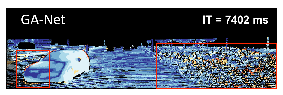
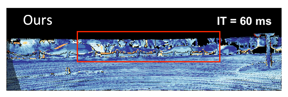
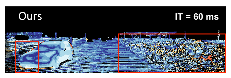
EPE: 
4.3. Benchmark Results
For benchmarking, we use our best performing network which is equipped with the AAHead and final hourglass refinement layer to evaluate on the KITTI 2015 test set on the official website. Table 4 shows the result of the evaluation in comparison to other models on the leader board. Compared to single-scale models our model achieves comparable results while reducing the complexity and run-time significantly. Compared to real-time models with inference time less than 100 milliseconds, our model achieves state-of-the-art results standing right beside the AANet+ (the improved variant of the original AANet) in D1 metric while having a lower memory and computational footprint and better scalability at the same inference time. The results in Tables 5 and 4 for both the KITTI 2015 and Sceneflow datasets demonstrate that our method maintains a balance between accuracy and speed. The iCFR algorithm thus can be applied to any state-of-the-art stereo matching architecture to make it more efficient and scalable while retaining its accuracy.
| D1-Noc | D1-All | Time | |||||
| Model | bg | fg | all | bg | fg | all | [ms] |
| GCNet (Kendall et al., 2017a) | 2.02 | 3.12 | 2.45 | 2.21 | 6.16 | 2.87 | 900 |
| PSMNet (Chang and Chen, 2018) | 1.71 | 4.31 | 2.14 | 1.86 | 4.62 | 2.32 | 410 |
| GANet (Zhang et al., 2019) | 1.34 | 3.11 | 1.63 | 1.48 | 3.46 | 1.81 | 1800 |
| StereoNet (Khamis et al., 2018) | - | - | - | 4.30 | 7.45 | 4.83 | 15 |
| DispNetC (Mayer et al., 2016) | 4.11 | 3.72 | 4.05 | 4.32 | 4.41 | 4.34 | 60 |
| DeepPruner-fast (Duggal et al., 2019) | 2.13 | 3.43 | 2.35 | 2.32 | 3.91 | 2.59 | 60 |
| AANet+ (Xu and Zhang, 2020) | 1.49 | 3.66 | 1.85 | 1.65 | 3.96 | 2.03 | 60 |
| FRSNet (Ours) | 1.58 | 3.45 | 1.88 | 1.73 | 3.87 | 2.09 | 60 |
| Models | EPE [px] | 3px [%] | Time [ms] |
|---|---|---|---|
| GCNet (Kendall et al., 2017a) | 2.51 | 9.34 | 950 |
| PSMNet (Chang and Chen, 2018) | 1.09 | 4.14 | 640 |
| GANet (Zhang et al., 2019) | 0.78 | - | 7402 |
| StereoNet (Khamis et al., 2018) | 1.10 | - | 15 |
| DispNetC (Mayer et al., 2016) | 1.68 | 9.31 | 60 |
| DeepPruner (Duggal et al., 2019) | 0.97 | - | 120 |
| AANet (Xu and Zhang, 2020) | 0.87 | 3.44 | 62 |
| FRSNet (Ours) | 0.93 | 6.01 | 60 |
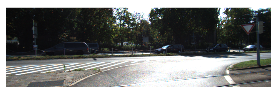
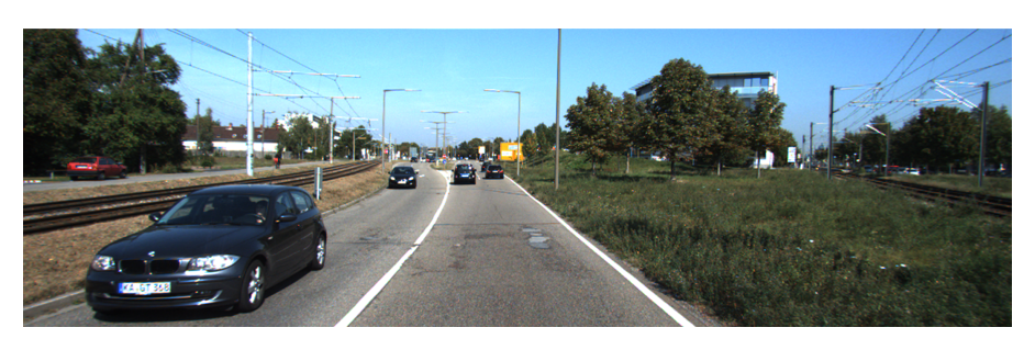
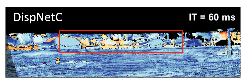
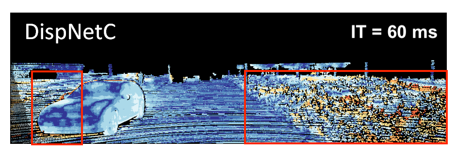
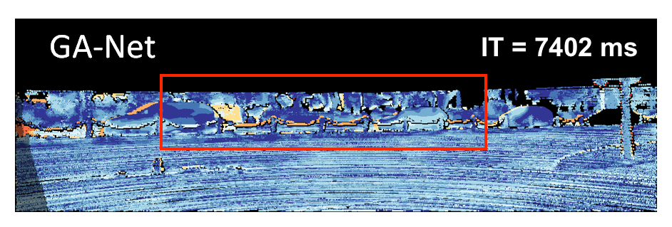
Figure 7 shows a comparison of D1 error maps produced by the KITTI 2015 benchmark on the test set. Our best performing model exhibits lower errors overall, especially at occluded areas and image boundaries. The error maps reveal even smaller errors on smooth regions. The maps also show that our model produces state-of-the-art results and outperforms other real-time models with visually consistent and continuous disparity maps.
5. Conclusion
In this paper, a novel multi-scale stereo matching architecture is proposed using the iCFR algorithm with disparity residuals. We show that our architecture can be applied to any state-of-the-art model to boost its efficiency in terms of run-time, memory, and scalability. We validate this on two state-of-the-art networks namely GANet (Zhang et al., 2019) and AANet (Xu and Zhang, 2020). Our best performing model performs 120x faster than the GANet and uses 5x less memory, using just 16% of FLOPs, while keeping the EPE and ER comparable. Our model scales until close to even 6K resolution on a GTX 1080Ti GPU, while keeping the inference time still below one second. The results show that by using iCFR, the trade-off between run-time and EPE can be optimized. Our best performing model produces state-of-the-art results on the Sceneflow test set as well as the KITTI 2015 benchmark while outperforming all the other real-time models in terms of accuracy.
Depending on the used prediction head and to keep the low, the proposed architecture has a limitation on the number of scales (or the maximum down-sampling factor) to use. This is because of the relation between the cost aggregation technique, the and scales as shown in Eq. 2.
An interesting future work would be extending our architecture with already fast prediction heads to see how much further the performance improvement can be pushed. We also hope that the considerable reduction in the number of FLOPs will make our model suitable for edge computing devices with real-time performance requirements.
Acknowledgements.
This work was partially funded by the Federal Ministry of Education and Research Germany under the project DECODE (01IW21001).References
- (1)
- Chabra et al. (2019) Rohan Chabra, Julian Straub, Christopher Sweeney, Richard Newcombe, and Henry Fuchs. 2019. Stereodrnet: Dilated residual stereonet. In Conference on Computer Vision and Pattern Recognition (CVPR).
- Chang and Chen (2018) Jia-Ren Chang and Yong-Sheng Chen. 2018. Pyramid stereo matching network. In Conference on Computer Vision and Pattern Recognition (CVPR).
- Chen et al. (2019) Rui Chen, Songfang Han, Jing Xu, and Hao Su. 2019. Point-based multi-view stereo network. In International Conference on Computer Vision (ICCV).
- Cheng et al. (2019) Xinjing Cheng, Peng Wang, and Ruigang Yang. 2019. Learning depth with convolutional spatial propagation network. Transactions on Pattern Analysis and Machine Intelligence (T-PAMI) (2019).
- Cheng et al. (2020) Xuelian Cheng, Yiran Zhong, Mehrtash Harandi, Yuchao Dai, Xiaojun Chang, Hongdong Li, Tom Drummond, and Zongyuan Ge. 2020. Hierarchical Neural Architecture Search for Deep Stereo Matching. Advances in Neural Information Processing Systems (NeurIPS) (2020).
- Duggal et al. (2019) Shivam Duggal, Shenlong Wang, Wei-Chiu Ma, Rui Hu, and Raquel Urtasun. 2019. DeepPruner: Learning efficient stereo matching via differentiable patchmatch. In International Conference on Computer Vision (ICCV).
- Falkenhagen (1997) Lutz Falkenhagen. 1997. Hierarchical block-based disparity estimation considering neighbourhood constraints. In International Workshop on SNHC and 3D Imaging.
- Geiger et al. (2012) Andreas Geiger, Philip Lenz, and Raquel Urtasun. 2012. Are we ready for autonomous driving? the kitti vision benchmark suite. In Conference on Computer Vision and Pattern Recognition (CVPR).
- Gu et al. (2020) Xiaodong Gu, Zhiwen Fan, Siyu Zhu, Zuozhuo Dai, Feitong Tan, and Ping Tan. 2020. Cascade cost volume for high-resolution multi-view stereo and stereo matching. In Conference on Computer Vision and Pattern Recognition (CVPR).
- Hirschmuller (2005) Heiko Hirschmuller. 2005. Accurate and efficient stereo processing by semi-global matching and mutual information. In Conference on Computer Vision and Pattern Recognition (CVPR).
- Jancosek and Pajdla (2009) Michal Jancosek and Tomás Pajdla. 2009. Segmentation based multi-view stereo. Citeseer.
- Kendall et al. (2017a) Alex Kendall, Hayk Martirosyan, Saumitro Dasgupta, Peter Henry, Ryan Kennedy, Abraham Bachrach, and Adam Bry. 2017a. End-to-end learning of geometry and context for deep stereo regression. In International Conference on Computer Vision (ICCV).
- Kendall et al. (2017b) Alex Kendall, Hayk Martirosyan, Saumitro Dasgupta, Peter Henry, Ryan Kennedy, Abraham Bachrach, and Adam Bry. 2017b. End-to-end learning of geometry and context for deep stereo regression. In International Conference on Computer Vision (ICCV).
- Khamis et al. (2018) Sameh Khamis, Sean Fanello, Christoph Rhemann, Adarsh Kowdle, Julien Valentin, and Shahram Izadi. 2018. StereoNet: Guided hierarchical refinement for real-time edge-aware depth prediction. In European Conference on Computer Vision (ECCV).
- Lin et al. (2017) Tsung-Yi Lin, Piotr Dollár, Ross Girshick, Kaiming He, Bharath Hariharan, and Serge Belongie. 2017. Feature pyramid networks for object detection. In Conference on Computer Vision and Pattern Recognition (CVPR).
- Liu et al. (2009) Yebin Liu, Xun Cao, Qionghai Dai, and Wenli Xu. 2009. Continuous depth estimation for multi-view stereo. In Conference on Computer Vision and Pattern Recognition (CVPR).
- Mayer et al. (2016) Nikolaus Mayer, Eddy Ilg, Philip Hausser, Philipp Fischer, Daniel Cremers, Alexey Dosovitskiy, and Thomas Brox. 2016. A large dataset to train convolutional networks for disparity, optical flow, and scene flow estimation. In Conference on Computer Vision and Pattern Recognition (CVPR).
- Min et al. (2011) Dongbo Min, Jiangbo Lu, and Minh N Do. 2011. A revisit to cost aggregation in stereo matching: How far can we reduce its computational redundancy?. In International Conference on Computer Vision (ICCV).
- Newell et al. (2016) Alejandro Newell, Kaiyu Yang, and Jia Deng. 2016. Stacked hourglass networks for human pose estimation. In European Conference on Computer Vision (ECCV).
- Pang et al. (2017) Jiahao Pang, Wenxiu Sun, Jimmy SJ Ren, Chengxi Yang, and Qiong Yan. 2017. Cascade residual learning: A two-stage convolutional neural network for stereo matching. In International Conference on Computer Vision Workshops (ICCVW).
- Schonberger et al. (2018) Johannes L Schonberger, Sudipta N Sinha, and Marc Pollefeys. 2018. Learning to fuse proposals from multiple scanline optimizations in semi-global matching. In European Conference on Computer Vision (ECCV).
- Tankovich et al. (2021) Vladimir Tankovich, Christian Hane, Yinda Zhang, Adarsh Kowdle, Sean Fanello, and Sofien Bouaziz. 2021. HITNet: Hierarchical iterative tile refinement network for real-time stereo matching. In Conference on Computer Vision and Pattern Recognition (CVPR).
- Xu and Zhang (2020) Haofei Xu and Juyong Zhang. 2020. AANet: Adaptive aggregation network for efficient stereo matching. In Conference on Computer Vision and Pattern Recognition (CVPR).
- Yang (2012) Qingxiong Yang. 2012. A non-local cost aggregation method for stereo matching. In Conference on Computer Vision and Pattern Recognition (CVPR).
- Yin et al. (2019) Zhichao Yin, Trevor Darrell, and Fisher Yu. 2019. Hierarchical discrete distribution decomposition for match density estimation. In Conference on Computer Vision and Pattern Recognition (CVPR).
- Yu and Gao (2020) Zehao Yu and Shenghua Gao. 2020. Fast-MVSnet: Sparse-to-dense multi-view stereo with learned propagation and gauss-newton refinement. In Conference on Computer Vision and Pattern Recognition (CVPR).
- Zbontar and LeCun (2015a) Jure Zbontar and Yann LeCun. 2015a. Computing the stereo matching cost with a convolutional neural network. In Conference on Computer Vision and Pattern Recognition (CVPR).
- Zbontar and LeCun (2015b) Jure Zbontar and Yann LeCun. 2015b. Computing the stereo matching cost with a convolutional neural network. In Conference on Computer Vision and Pattern Recognition (CVPR).
- Zhang et al. (2019) Feihu Zhang, Victor Prisacariu, Ruigang Yang, and Philip HS Torr. 2019. GA-Net: Guided aggregation net for end-to-end stereo matching. In Conference on Computer Vision and Pattern Recognition (CVPR).
- Zhang and Liu (2014) Xiaoxue Zhang and Zhigang Liu. 2014. A survey on stereo vision matching algorithms. In World Congress on Intelligent Control and Automation (WCICA).
- Zhu et al. (2019) Xizhou Zhu, Han Hu, Stephen Lin, and Jifeng Dai. 2019. Deformable convnets v2: More deformable, better results. In Conference on Computer Vision and Pattern Recognition (CVPR).