Index of Embedded Networks in the Sphere

Abstract

In this paper, we will compute the Morse index and nullity for the stationary embedded networks in spheres. The key theorem in the computation is that the index (and nullity) for the whole network is related to the index (and nullity) of small networks and the Dirichlet-to-Neumann map defined in this paper. Finally, we will show that for all stationary triple junction networks in $\mathbb{S}^{2}$, there is only one eigenvalue (without multiplicity) $-1$, which is less than 0, and the corresponding eigenfunctions are locally constant. Besides, the multiplicity of eigenvalues 0 is 3 for these networks, and their eigenfunctions are generated by the rotations on the sphere.

1 Introduction

As a one-dimensional singular version of surfaces, the networks always attract a lot of researchers. In the study of minimal surfaces and mean curvature flows, especially in the case with singularities, networks are always considered first since they are simple enough for analysis but still could give some useful results. Probably one of the famous stories is a group of undergraduate students [3] gave the proof of the 2-dimensional analog of the double bubble conjecture. Later on, F. Morgan and W. Wichiramala [17] extended their result and showed the unique stable double bubble in $\mathbb{R}^{2}$ is the standard double bubble. There are also extensive researches about the planar clusters. See for example [2, 16, 9, 25]. In particular, one can also find the nice and elementary introduction of planar clusters in [14, 15].

Similarly, since the mean curvature flows of surfaces with junctions are hard, there are also a lot of works regarding the one-dimensional mean curvature flows for networks, namely network flows. See for instance [18, 12, 1, 10, 21] for some results of mean curvature flows with triple junctions and network flows.

Besides that, the Morse index is an important concept for minimal surfaces. In general, it is pretty hard to calculate the index of a general minimal surface in general ambient spaces, especially the minimal surfaces generated by Almgren-Pitts min-max theory, see for instance [23, 4, 13, 11, 7] (including the free boundary minimal surfaces case).

After the work [24], we are interested in more things about minimal multiple junction surfaces, especially the Morse index of those surfaces. Unfortunately, we might need to do a lot of analysis of elliptic operators on the multiple junction surfaces, especially the regularity. So before that, we can try to consider calculating the index of one-dimensional multiple junction surfaces to see if we can find a good method to compute the index. In this paper, we will focus on the Morse index and nullity of triple junction networks, especially when they are minimally embedded in $\mathbb{S}^{2}$.

Before the computation, we need the definitions of stationary networks on $\mathbb{S}^{2}$. The precise definitions and related notations will be described in Section 2. Here we give a quick introduction so we can state the main theorem. At first, we will need to calculate its first and second variations. This will lead to the function spaces and stability operators we’re interested in on this network. Indeed, similar things have been done in my previous work [24]. So for the functions defined on the network, we still need a compatible condition (see Subsection 2.2 for detailed function spaces) to make sure it can arise from the variation on $\mathbb{S}^{2}$. The stability operator just has form

$$Lu=\Delta u+u$$

by the second variation of networks. So this operator is closely related to the Laplacian operator on the network. This is one difference with the case of the minimal surfaces since there are usually more terms related to the second fundamental form of surfaces in the stability operators.

After giving the elliptic operator on the network, we can talk about its eigenvalues and eigenfunctions on this network related to operator $L$. Standard methods and results about the spectrum of elliptic operators from PDEs can directly be applied to the operator $L$ here, especially the min-max characterization of eigenvalues. Until now, we can define the (Morse) index and nullity of the network in the sphere.

Now we can state our first main theorem of index and nullity of embedded stationary triple junction networks in $\mathbb{S}^{2}$ (see Theorem 5.1 for more precise statement).

Theorem 1.1 (Index and nullity of stationary triple junction networks).

The Morse index of all embedded closed stationary triple junction networks in $\mathbb{S}^{2}$ is $F-1$ where $F$ is the number of regions on sphere cut by this network. The corresponding eigenfunctions are all locally constants(explained in Theorem 5.1) with eigenvalue $-1$.

The nullity of all embedded closed stationary triple junction networks in $\mathbb{S}^{2}$ is 3 and the corresponding eigenfunctions are generated by the rotations on $\mathbb{S}^{2}$ with eigenvalue $0$.

In other words, this theorem says that there is a gap (0 and 1) between the first two eigenvalues (without multiplicity) of the Laplacian operator. Recall that the outstanding open problem from S.T.Yau [26] says the first non-trivial eigenvalue of the Laplacian on a closed embedded minimal hypersurface in $\mathbb{S}^{n}$ is $n$. This conjecture is far from solved (see for instance [19, 27]). Our theorem says that Yau’s conjecture is true for one-dimensional stationary triple junction networks under our scenarios of the above theorem. So it will give partial results related to Yau’s conjecture.

The proof of Theorem 1.1 require the classification of embedded closed stationary triple junction networks in $\mathbb{S}^{2}$. If we do not assume the networks to have junction order at most three at each junction point, then there are infinitely many stationary embedded networks in $\mathbb{S}^{2}$, although they aren’t area-minimizing locally in the sense of sets.

Usually, it is relatively hard to direct compute the networks’ index and nullity just based on the definitions. Inspired by the work of H. Tran [22], we can consider dividing the big network into several small parts and to see if we can calculate the index and nullity through the index and nullity of a small network and a suitable Dirichlet-to-Neumann map. It turns out this method works for the networks. So this part is the central part of this paper. It will provide a vital tool in the calculation, although we need a bit more space to give the definition of the Dirichlet-to-Neumann map for a network with boundary. The eigenvalues of the Dirichlet-to-Neumann map are known as the Steklov eigenvalues. There is also quite a lot of research related to the Steklov eigenvalues, and they have a relationship with minimal surfaces, too. For example, Fraser and Schoen [5, 6] gave the relation between extremal Steklov eigenvalues and free boundary minimal surfaces in a ball.

Now suppose we cut a big network into small pieces along a finite point set $\overline{\mathcal{P}}$. Then we can define a new Dirichlet-to-Neumann map $\overline{T}$ on set $\overline{\mathcal{P}}$ using the Dirichlet-to-Neumann map constructed on small networks. The precise definition is given in Section 4. Using this Dirichlet-to-Neumann map, we have the following index and nullity theorem to calculate the index and nullity for a big network (see Theorem 4.1 and Theorem 4.3 for details).

Theorem 1.2 (Index and nullity theorem).

The nullity of a big network is the sum of the following numbers

• The nullity of $\overline{T}$.

• The dimension of space of functions that have eigenvalue 0 when restricted on each small network and happen to be the eigenfunctions with eigenvalue 0 on the big network.

The index of a big network is the sum of the following numbers

• Index of each small network.

• Index of Dirichlet-to-Neumann $\overline{T}$.

• The dimension of space of functions that has eigenvalue 0 when restricted on each small network but orthogonal to the function space mentioned in the nullity part.

Although the key thought comes from the work [22], there are still some differences from the cases of the free boundary surfaces. The first thing is, the properties of elliptic operators on the network are quite different from the usual elliptic operators on the surface. So we need to pay more attention to how to define the Dirichlet-to-Neumann map for each small network. Then we can try to construct a global Dirichlet-to-Neumann map $\overline{T}$ from the Dirichlet-to-Neumann on the small networks along the junctions. In the definition of $\overline{T}$, we need to make sure $\overline{T}$ can agree with the usual Dirichlet-to-Neumann on subnetworks and also require every function in the image of $\overline{T}$ will still lie the function space we care about. So we will define quite a lot of spaces to make sure $\overline{T}$ is well-defined.

As a corollary of Theorem 1.2 (see Corollary 4.4), we know the number of eigenvalues not greater than 0 (count multiplicity) of a big network is just the sum of all eigenvalues not greater than 0 of the small networks and Dirichlet-to-Neumann $\overline{T}$. This corollary will help us to calculate the index and nullity of complex networks on $\mathbb{S}^{2}$.

Remark.

We believe this theorem can be extended to higher dimensions for surface clusters like the minimal multiple junction surfaces mentioned in [24]. This will help us to calculate the Morse index for some special minimal triple junction surfaces. We will investigate this direction in future work.

In Section 2, we will give the basic definitions of networks in $\mathbb{S}^{2}$ and their indexes and nullities. Then we will talk about the eigenvalues and eigenfunctions from the aspect of elliptic partial differential equations in Section 3, including the definition of Dirichlet-to-Neumann on the network with boundary. In Section 4, we will given the new Dirichlet-to-Neumann map for the partition of networks and prove the main Theorem 1.2. In the last section, we will calculate the index and nullity of embedded closed stationary triple junction networks to finish the proof of Theorem 1.1.

2 Preliminary

2.1 Curves and networks in $\mathbb{S}^{2}$

We say $\gamma:I\rightarrow\mathbb{S}^{2}$ is a (smooth) curve if $\gamma$ is a smooth map from an interval $I$ to $\mathbb{S}^{2}$. Sometimes, we call a subset of $\mathbb{S}^{2}$ is a curve if this subset is an image of a curve $\gamma$.

We make the following definitions and assumptions for curves we’re interested in.

• A curve $\gamma$ is called regular if $\gamma^{\prime}(t)\neq 0$ for every $t\in I$. When we talk about a curve in this paper, we will always assume it is regular.

• We define $\xi(t)=\frac{\gamma^{\prime}(t)}{\left|\gamma^{\prime}(t)\right|}$ to be the unit tangent vector field along regular curve $\gamma$.

• We write $\nu(t)$ to be the unit normal vector field along a curve $\gamma$.

• We write $\tau$ as the unit outer normal of $\gamma$. That means $\tau$ is only defined at $\gamma(0)$ and $\gamma(1)$ with $\tau(\gamma(0))=-\xi(0),\tau(\gamma(1))=\xi(1)$.

• Although $I$ can be unbounded, we will only consider $I$ is a bounded closed interval. Moreover, we can assume $I=[0,1]$ after reparametrization.

• We will assume all curves in this paper does not have self-intersection. That is $\gamma(t_{1})\neq\gamma(t_{2})$ for any $0\leq t_{1}<t_{2}\leq 1$.

• The Length of $\gamma$, written as $L(\gamma)$, is defined as

  $$L(\gamma):=\int_{I}\left|\gamma^{\prime}(t)\right|dt$$

Definition 2.1.

A network in $\mathbb{S}^{2}$ with interior endpoints set $\mathcal{P}$ and boundary endpoints set $\mathcal{Q}$ is defined as a collection of finite curves $\{\gamma^{1},\cdots,\gamma^{n}\}$ in $\mathbb{S}^{2}$ such that

• $\mathcal{P},\mathcal{Q}\subset\mathbb{S}^{2}$ are two finite point sets such that $\mathcal{P}\cap\mathcal{Q}=\emptyset$.

• $\mathcal{P}\cup\mathcal{Q}$ is the set of all possible (distinct) endpoints of $\gamma^{i}$ for $i=1,\cdots,n$. That is $\mathcal{P}\cup\mathcal{Q}=\bigcup_{i=1}^{n}\{\gamma^{i}(0),\gamma^{i}(1)\}$.

We say a network $\mathcal{N}$ is embedded if $\gamma^{i}$ can only intersect each other at their endpoints. We will always assume $\mathcal{N}$ is embedded in $\mathbb{S}^{2}$ unless we say it is immersed.

For any $P\in\mathcal{P}$, we write $\{\gamma^{j}_{P}\}_{j=1,\cdots,j_{P}}$ as the collection of $\gamma^{i}$ having $P$ as its endpoint. We write $\tau^{j}_{P}$ as the exterior unit tangent vector of $\gamma^{j}_{P}$ for $j=1,\cdots,j_{P}$. For example, if $\gamma^{j}_{P}(0)=P$, then $\tau^{j}_{P}=-\frac{(\gamma^{j}_{P})^{\prime}(0)}{\left|(\gamma^{j}_{P})^{\prime}(0)\right|}$.

Similarly, for any $Q\in\mathcal{Q}$, we write $\{\gamma^{k}_{Q}\}_{k=1,\cdots,k_{Q}}$ as the collection of $\gamma^{i}$ having $Q$ as its endpoint and use $\tau^{k}_{Q}$ to denote the exterior unit tangent vector of $\gamma_{Q}^{k}$. In most cases of this paper, $k_{Q}$ will be one, and we write $\gamma_{Q}=\gamma^{1}_{Q}$ for short.

To avoid ambiguity, we suppose $\tau^{j}_{P}(\tau^{k}_{Q})$ pointing different directions for each $P\in\mathcal{P}(Q\in\mathcal{Q})$.

We say a network $\mathcal{N}$ is closed if $Q=\emptyset$.

Remark.

Of course, we can define the networks in the general manifold or even define the network intrinsically by identifying their endpoints. We can see most of the arguments can go through even if for the intrinsic definitions.

Definition 2.2.

We say $\mathcal{N}$ is a stationary network in $\mathbb{S}^{2}$ if the following hold.

• Each $\gamma^{i}$ is an arc of a great circle.

• For any $P$ in $\mathcal{P}$, we have

  $$\sum_{j=1}^{j_{P}}\tau_{P}^{j}=0$$

Remark.

If $\mathcal{N}$ is stationary, then we know all of $j_{P}\geq 2$ by the second condition in the definition.

Remark.

We can also consider the network with density $\theta_{i}$ at each $\gamma^{i}$ like [24]. By imposing appropriate densities, we can see that the one skeleton of the spherical truncated icosahedron(soccer ball) can be stationary. So it is possible to calculate the index and nullity for this kind of network.

By a simple geometric observation, we know for the stationary network $\mathcal{N}$, the following two special cases hold. Let $P\in\mathcal{P}$, then

• If $P$ is a double endpoint, i.e. $j_{P}=2$, then $\tau^{1}_{P}=-\tau^{2}_{P}$ as a vector.

• If $P$ is a triple endpoint, i.e. $j_{P}=3$, then $\tau^{1}_{P}+\tau^{2}_{P}+\tau^{3}_{P}=0$ as a vector.

We can define the total length of $\mathcal{N}$, written as $L(\mathcal{N})$, as the sum of all $\gamma^{i}$. That is

$$L(\mathcal{N}):=\sum_{i=1}^{n}L(\gamma^{i})$$

Like the minimal surfaces, we have the first variation formula for the length of $\mathcal{N}$. Suppose $\mathcal{N}_{t}=\{\gamma^{i}_{t}\}_{i=1}^{n}$ to be a smooth variation of $\mathcal{N}$ fixing $\mathcal{Q}$, then

$$\left.\frac{d}{dt}\right|_{t=0}L(\mathcal{N}_{t})=\sum_{i=1}^{n}\int_{\gamma^{i}}\kappa^{i}\nu^{i}\cdot Xds^{i}+\sum_{P\in\mathcal{P}}\sum_{j=1}^{j_{P}}X\cdot\tau_{P}^{j}$$

where $\kappa^{i}$, the geodesic curvature of $\gamma^{i}$ in $\mathbb{S}^{2}$ with respect to $\nu^{i}$, $\nu^{i}=\nu^{\gamma^{i}}$, the unit normal vector field along $\gamma^{i}$, $X$, a variational vector field associating with variation of $\mathcal{N}$.

From the first variation formula, we can see that $\mathcal{N}$ is a stationary network in $\mathbb{S}^{2}$ if and only if it is a critical point of length for any suitable variation $\mathcal{N}_{t}$.

Similarly, we can compute the second variation formula. Suppose $\mathcal{N}$ is a stationary network. If we write $\phi^{i}=X\cdot\nu^{i}$, then the second derivative of length can be computed by

$$\left.\frac{d^{2}}{dt^{2}}\right|_{t=0}L(\mathcal{N}_{t})=\sum_{i=1}^{n}\int_{\gamma^{i}}\left|\nabla^{\gamma^{i}}\phi^{i}\right|^{2}-\left|\phi^{i}\right|^{2}ds^{i}$$

where $\nabla^{\gamma^{i}}$ is the gradient on $\gamma^{i}$.

So we can say $\mathcal{N}$ is stable if $\left.\frac{d^{2}}{dt^{2}}\right|_{t=0}L(\mathcal{N}_{t})\geq 0$ for any variation $\mathcal{N}_{t}$ fixing $\mathcal{Q}$.

2.2 Some useful function spaces

Based on the properties of $\phi^{i}$, we define the following function spaces on $\mathcal{N}$.

Definition 2.3.

When we say $\phi$ is a function on $\mathcal{N}$, we mean $\phi$ is a tuple $(\phi^{1},\cdots,\phi^{n})$ that each $\phi^{i}$ is a function defined on $\gamma^{i}$.

We say a function $\phi$ defined on $\mathcal{N}$ is in $C^{k}(\mathcal{N})$ ($k\in\mathbb{N}\cup\{\infty\}$) function space if $\phi^{i}$ is a $C^{k}(\gamma^{i})$ function on $\gamma^{i}$.

Similarly, we have the Sobolev space on $\mathcal{N}$ defined by following.

Definition 2.4.

We say a function $\phi$ defined on $\mathcal{N}$ is in $W^{k,p}(\mathcal{N})$ function space if the restriction $\phi^{i}$ is a $W^{k,p}$ function on $\gamma^{i}$.

Now suppose we have a $C^{k}$ (tangential) vector field on $\mathbb{S}^{2}$, then we can define a $C^{k}(\mathcal{N})$ function by defining $\phi$ by taking $\phi^{i}=X\cdot\nu^{i}$. We will write this function $\phi=X\cdot\nu$ for short. Besides, for any $C^{k}$ function $f$ on $\mathbb{S}^{2}$, we know the function $\phi$ defined by $\phi^{i}:=f|_{\gamma^{i}}$ is a $C^{k}(\mathcal{N})$ function. So we know $C^{k}(\mathcal{N})$ function space is quite large. Since we are interested in the functions in the form $\phi=X\cdot\nu$, let’s define a subspace of $C^{k}(\mathcal{N})$ in the following ways.

Definition 2.5.

We say a function $\phi\in C^{k}_{1}(\mathcal{N})$ if for any $P\in\mathcal{P}$, there exists a vector $X\in T_{P}\mathbb{S}^{2}$ such that $\phi^{j}_{P}=X\cdot\nu^{\gamma^{j}_{P}}$ at $P$. Here we use $\phi^{j}_{P}:=\phi^{i}$ such that $\gamma^{i}=\gamma^{j}_{P}$.

Similarly, we have a version like Sobolev spaces.

Definition 2.6.

We say a function $\phi\in W^{k,p}_{1}(\mathcal{N})$, $k\geq 1$ if for any $P\in\mathcal{P}$, there exists a vector $X\in T_{P}\mathbb{S}^{2}$ such that $\phi_{P}^{j}=X\cdot\nu^{\gamma^{j}_{P}}$ at $P$. Here the restriction of $\phi^{j}_{P}$ at $P$ should be understood in the trace sense.

We can easily check $W^{k,p}_{1}(\mathcal{N})$ is a closed subspace of $W^{k,p}(\gamma^{1})\times\cdots\times W^{k,p}(\gamma^{n})$ with product norm, so $W^{k,p}_{1}(\mathcal{N})$ is a Sobolev space.

Here we introduce other notations to present these function spaces. For any $P\in\mathcal{P}$, we define $V(P):=\mathbb{R}^{j_{P}}$ as a vector space with $\mathrm{dim}=j_{P}$. Note that when given a function $\phi\in C^{k}(\mathcal{N})$, the restriction of $\phi$ on $P$ is just a tuple $(\gamma^{1}_{P}|_{P},\cdots,\gamma^{j_{P}}_{P}|_{P})$, which can be viewed as an element in $V(P)$. So $V(P)$ is just like a function space on $P$, which comes from the restriction of functions on $\mathcal{N}$. Now we define $V_{1}(P):=\{(v_{1},\cdots,v_{j_{P}})\in V(P):v_{j}=X\cdot\nu^{j}_{P},\quad\forall 1\leq j\leq j_{P}\text{ for some }X\in T_{P}\mathbb{S}^{2}\}$. $V_{1}(P)$ is a subspace of $V(P)$ with dimension at most $2$.

Then we can define $V(\mathring{\mathcal{P}}):=\bigoplus_{P\in\mathring{\mathcal{P}}}V(P),V_{1}(\mathring{\mathcal{P}}):=\bigoplus_{P\in\mathring{\mathcal{P}}}V_{1}(P)$ for any $\mathring{\mathcal{P}}\subset\mathcal{P}$. With these notations, we know a function $\phi\in C^{k}(\mathcal{N})(\phi\in W^{k,p}(\mathcal{N}))$ is in the space $C^{k}_{1}(\mathcal{N})(\phi\in W^{k,p}_{1}(\mathcal{N}))$ if and only if $\phi|_{\mathcal{P}}\in V_{1}(\mathcal{P})$.

Besides, we introduce another subspace of $V(\mathcal{P})$ that we will use later on. We define $V_{2}(P):=V_{1}^{\bot}(P)$ for any $P\in\mathcal{P}$ and write $V_{2}(\mathring{\mathcal{P}}):=\bigoplus_{P\in\mathring{\mathcal{P}}}V_{2}(P)$ for any $\mathring{\mathcal{P}}\subset\mathcal{P}$ where the inner product on $V(\mathcal{P}_{1})$ is the standard Euclid inner product.

Another helpful function space is the space of trace zero functions. We define $W^{k,p}_{0}(\mathcal{N})$ as the trace zero function space. That is, $W^{k,p}_{0}(\mathcal{N}):=\{\phi\in W^{k,p}(\mathcal{N}):\phi=0\text{ on }\mathcal{Q}\}$. We will write $W^{k,p}_{0,1}(\mathcal{N}):=W^{k,p}_{0}(\mathcal{N})\cap W^{k,p}_{1}(\mathcal{N})$ for short.

Similarly, we write $C^{k}_{0}(\mathcal{N})$ as the functions in $C^{k}(\mathcal{N})$ with zero boundary values. We write $C^{k}_{0,1}(\mathcal{N}):=C^{k}_{0}(\mathcal{N})\cap C^{k}_{1}(\mathcal{N})$.

Note that in the above, when we write $\phi=0$ on $\mathcal{Q}$, we actually mean $\phi^{k_{i}}_{Q}=0$ at $Q$ for $i=1,\cdots,k_{Q}$ for all $Q\in\mathcal{Q}$. This means when we restrict $\phi$ on $\mathcal{Q}$, this restriction is just like a vector with dimension $\sum_{Q\in\mathcal{Q}}k_{Q}$. For convenience, we write $V(\mathcal{Q}):=\bigoplus_{Q\in\mathcal{Q}}\mathbb{R}^{k_{Q}}$ as the function space defined on $\mathcal{Q}$.

From these definitions, we know the function $X\cdot\nu$ is a $C^{k}_{1}(\mathcal{N})$ function if $X$ is a $C^{k}$ vector field on $\mathbb{S}^{2}$.

Remark.

In general, given $\phi\in C_{1}^{k}(\mathcal{N})$, one may not find a $C^{k}$ vector field $X$ on $\mathbb{S}^{2}$ such that $\phi^{i}=X\cdot\nu^{i}$.

In the previous definitions of $C^{k}_{1}(\mathcal{N})$ and $W^{k,p}_{1}(\mathcal{N})$, for $\mathcal{N}$ being a stationary network, if $P$ is a double endpoint or a triple endpoint, and the choice of $\nu^{j}$ on $\gamma^{j}$ satisfies $\sum_{j=1}^{j_{P}}\nu^{\gamma^{j}_{P}}=0$, then the condition for $\phi$ can be simplified by

$$\sum_{j=1}^{j_{P}}\phi^{j}_{P}=0,\quad j_{P}=2\text{ or }j_{P}=3.$$

Following from the index form for minimal surfaces, we can define the index form for $W^{1,2}_{0,1}(\mathcal{N})$ functions. Let $\mathcal{N}$ be a stationary network in $\mathbb{S}^{2}$. From the second variation formula, we can define the bilinear form, called the index form, by the following. For any $\phi,\psi\in W^{1,2}_{0,1}(\mathcal{N})$, let

$$Q(\phi,\psi):=\sum_{i=1}^{n}\int_{\gamma^{i}}\nabla^{\gamma^{i}}\phi^{i}\cdot\nabla^{\gamma^{i}}\psi^{i}-\phi^{i}\psi^{i}ds^{i}.$$

To simplify our formulas, we use the following notations. For any $\phi\in W^{k,p}_{1}(\mathcal{N})$ (and hence $C_{1}^{k}(\mathcal{N})$),

$$\int_{\mathcal{N}}\phi:={} \sum_{i=1}^{n}\int_{\gamma^{i}}\phi^{i}ds^{i}$$

$$\int_{\mathcal{P}}\phi:={} \sum_{P\in\mathcal{P}}\sum_{j=1}^{j_{P}}\left.\phi^{j}_{P}\right|_{P}=\sum_{i=1}^{n}\left(\phi^{i}(0)+\phi^{i}(1)\right)$$

The integral of $\phi$ on $\mathcal{P}$ is just the summation of all $\phi^{i}$ taking values at endpoints.

So the index form can be written as

$$Q(\phi,\psi)=\int_{\mathcal{N}}\nabla\phi\cdot\nabla\psi-\phi\psi=-\int_{\mathcal{N}}\phi\left(\Delta\psi+\psi\right)+\int_{\mathcal{P}}\phi\frac{\partial}{\partial\tau}\psi.$$

where we’ve assumed $\phi,\psi\in C^{k}_{0,1}(\mathcal{N})$ for $k\geq 2$ for the last identity. Besides, with the above notation, $\int_{\mathcal{P}}\phi\frac{\partial}{\partial\tau}\psi$ should be understood as

$$\sum_{P\in\mathcal{P}}\sum_{j=1}^{j_{P}}\left.\phi^{j}_{P}\right|_{P}\frac{\partial}{\partial\tau^{j}_{P}}\psi^{j}_{P}$$

For any $\phi\in C^{k}_{1}(\mathcal{N})$ for $k\geq 2$, we can define the operator $L\phi$ by

$$(L\phi)^{i}:=\Delta_{\gamma^{i}}\phi^{i}+\phi^{i}\quad(\text{Write it as }L\phi=\Delta\phi+\phi\text{ for short.})$$

We can rewrite $Q$ as $Q(\phi,\psi)=-\int_{\mathcal{N}}\phi L\psi+\int_{\mathcal{P}}\phi\frac{\partial}{\partial\tau}\psi$.

Remark.

The Laplacian in the index form is just the usual second derivative of a function with arc-length parameterization. One can try to define the index form for some particular clusters of minimal surfaces like minimal multiple junction surfaces defined in [24].

Now we can define the Morse index and nullity of $Q$ for a stationary network $\mathcal{N}$.

Definition 2.7.

The Morse index of a stationary network $\mathcal{N}$, written as $\mathrm{Ind}(\mathcal{N})$, is defined to be the maximal dimension of a subspace of $W^{1,2}_{0,1}(\mathcal{N})$ which the quadratic form $Q$ is negative-defined.

Similarly, the nullity of $\mathcal{N}$, written as $\mathrm{Nul}(\mathcal{N})$, is defined as the maximal dimension of a subspace of $W^{1,2}_{0,1}(\mathcal{N})$ which the quadratic form $Q$ vanishes.

Considering the case of the usual symmetric elliptic operator, we can define the spectrum of an operator $L$.

Definition 2.8.

We say $\lambda\in\mathbb{R}$ is a weak eigenvalue of $L$ if there is a function $\phi\in W^{1,2}_{0,1}(\mathcal{N})$ such that

$$Q(\phi,\psi)=\lambda\int_{\mathcal{N}}\phi\psi$$

for all $\psi\in W^{1,2}_{0,1}(\mathcal{N})$. The function $\phi$ is called the weak eigenfunction of $L$ with eigenvalue $\lambda$.

In general, we need to develop the regularity theorems to show the eigenfunction $\phi\in C^{\infty}_{0,1}(\mathcal{N})$. But for the 1-dimensional case, we can easily show $\phi\in C^{\infty}_{0,1}(\mathcal{N})$. Indeed, if $\phi$ is an eigenfunction, then on each curve $\gamma^{i}$, $\phi^{i}$ is Höder continuous by Morrey’s inequality. So at least we know $\phi\in C^{0}_{0,1}(\mathcal{N})$. Note that $\phi^{i}$ satisfies $-\Delta u-u=\lambda u$ weakly on $\gamma^{i}$ with Dirichlet condition $u=\phi^{i}$ at $\gamma^{i}(0)$ and $\gamma^{i}(1)$, so $\phi^{i}$ is a smooth function up to the boundary by the usual regularity theorem for the Dirichlet problems. Hence $\phi\in C^{\infty}_{0,1}(\mathcal{N})$. Now we need to introduce another condition on function spaces to describe the properties of eigenfunctions. We say a function $\phi\in C^{k}_{1}(\mathcal{N})$, $k\geq 1$, (or $\phi\in W^{k,p}_{1}(\mathcal{N}),k\geq 2$) satisfies the compatible condition at $P$ if the following equations hold

$$\sum_{j=1}^{j_{P}}X\cdot\nu^{\gamma^{j}_{P}}\frac{\partial}{\partial\tau^{j}_{P}}\phi^{j}_{P}=0\text{ for all }X\in T_{P}\mathbb{S}^{2}\text{ at }P$$

We say a function $\phi\in C^{k}_{1}(\mathcal{N})$, $k\geq 1$, (or $\phi\in W^{k,p}_{1}(\mathcal{N}),k\geq 2$)satisfies the compatible condition if $\phi$ satisfies the compatible condition at each $P$ for any $P\in\mathcal{P}$.

Note that $X\cdot\nu^{\gamma^{j}_{P}}\in V_{1}(P)$, then $\phi$ satisfies the compatible condition at $P$ if and only if $(\frac{\partial}{\partial\tau_{P}^{j}}\phi^{j}_{P})_{j=1}^{j_{P}}\in V_{2}(P)$. So $\phi$ satisfies the compatible condition on $\mathcal{P}$ if and only if $\frac{\partial}{\partial\tau}\phi\in V_{2}(\mathcal{P})$ in short notation. In some special cases, this compatible condition will become much simple, which will help us to understand what this condition says. If at $P$, we have $j_{P}=2$ or $3$(double or triple junction) and $\sum_{j=1}^{j_{P}}\nu^{\gamma^{j}_{P}}=0$, then the compatible condition at $P$ is equivalent to the condition

$$\frac{\partial}{\partial\tau^{j}_{P}}\phi^{j}_{P}=\frac{\partial}{\partial\tau^{k}_{P}}\phi^{k}_{P},\quad\forall 1\leq j,k\leq j_{P}\text{ at }P.$$

With these conditions, we can describe another definition of eigenvalues and eigenfunctions.

Definition 2.9.

We say $\lambda\in\mathbb{R}$ is an eigenvalue of $L$ if there is a function $\phi\in C^{\infty}_{0,1}(\mathcal{N})$ which satisfies the compatible condition on $\mathcal{P}$ such that

$$-L\phi=\lambda\phi.$$

The function $\phi$ is called the eigenfunction of $L$ with eigenvalue $\lambda$.

Using the integrate by part and regularity results above, we know $\lambda\ (\phi)$ is an eigenvalue (an eigenfunction) if and only if it is a weak eigenvalue (a weak eigenfunction).

Remark.

From the definitions in this subsection, we know the function space $C^{\infty}_{0,1}(\mathcal{N})$ only relies on the choice of $V_{1}(P)$ for each $P\in\mathcal{P}$. So if we want to define the function space $C^{\infty}_{0,1}(\mathcal{N})$ for intrinsic networks, we only need to choose a suitable function space $V_{1}(P)$ for each $P$. This will allow us to define the general elliptic operator acts on space $W^{\infty}_{0,1}(\mathcal{N})$, which does not rely on the embedding.

Besides, we can consider the general operator $Lu=\Delta u+du$ where $d\in C^{\infty}(\mathcal{N})$. So we will always use operator $L$ instead of $\Delta+1$ to indicate they can be generalized.

2.3 Examples of eigenfunctions

Here we give an example of a stationary network. From this example, we will illustrate what the space $C^{k}_{1}(\mathcal{N})$ looks like and which conditions that eigenfunctions should satisfy.

Let $\mathcal{N}$ be the one-skeleton of a regular spherical tetrahedron like the one shown in Figure 1.

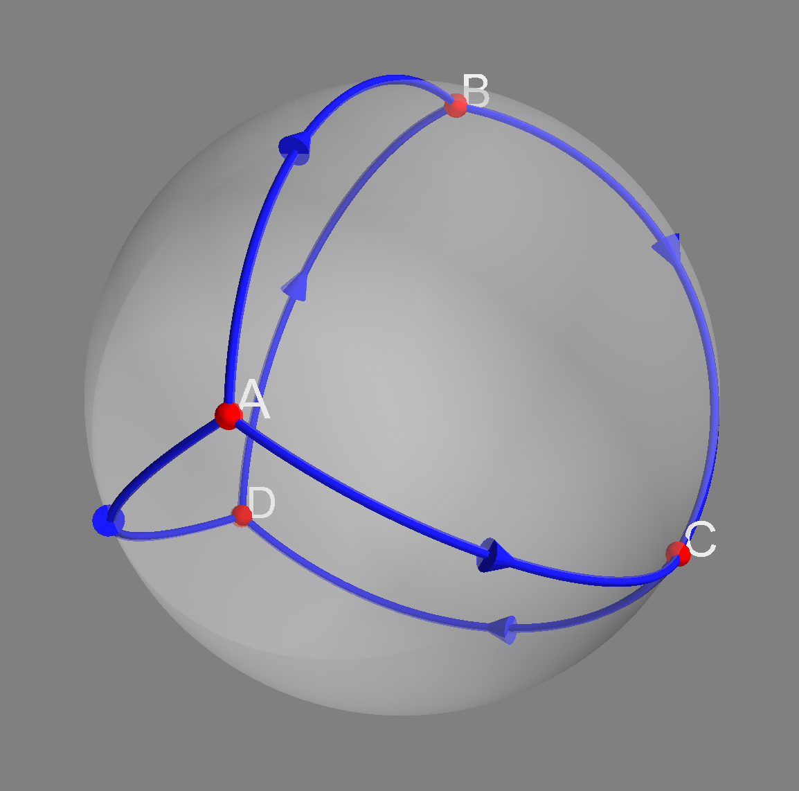
(a) $\mathcal{N}$ on the sphere

(b) Stereographic projection of $\mathcal{N}$

Figure 1: A regular spherical tetrahedron

$\mathcal{N}$ has six arcs with orientation shown in Figure 1(b). So for a function $\phi\in C^{k}(\mathcal{N})$, $\phi$ belongs to $C_{1}^{k}(\mathcal{N})$ if and only if the following holds

$$\begin{cases}\phi^{1}(0)+\phi^{2}(0)+\phi^{3}(0)=0,&\\ \phi^{1}(1)-\phi^{5}(0)+\phi^{6}(1)=0,&\\ \phi^{2}(1)-\phi^{6}(0)+\phi^{4}(1)=0,\\ \phi^{3}(1)-\phi^{4}(0)+\phi^{5}(1)=0.\end{cases}$$ (1)

Let $l=\cos^{-1}(-\frac{1}{3})$ be the length of arcs in $\mathcal{N}$. Then the function $\phi$ becomes an eigenfunction with eigenvalue $\lambda$ if and only if the following holds,

$$\begin{cases}-\frac{1}{l^{2}}(\phi^{i})^{\prime\prime}-\phi^{i}=\lambda\phi^{i},&\text{ for }i=1,\cdots,6\\ (\phi^{1})^{\prime}(0)=(\phi^{2})^{\prime}(0)=(\phi^{3})^{\prime}(0),&\\ (\phi^{1})^{\prime}(1)=(\phi^{5})^{\prime}(0)=(\phi^{6})^{\prime}(1),&\\ (\phi^{2})^{\prime}(1)=(\phi^{6})^{\prime}(0)=(\phi^{4})^{\prime}(1),\\ (\phi^{3})^{\prime}(1)=(\phi^{4})^{\prime}(0)=(\phi^{5})^{\prime}(1).\end{cases}$$ (2)

Here, we’ve assumed the length of $(\gamma^{i})^{\prime}$ is constant for each $i$. By minimizing the Rayleigh quotient, we know the lowest eigenvalue should be $-1$, and the corresponding eigenfunction should be constant on each $\gamma^{i}$. Suppose $\phi$ is such function. This means we suppose $\phi^{i}=c^{i}$, which is a constant on $\gamma^{i}$. The condition (2) holds automatically with $\lambda=-1$, and the condition (1) will become

$$\begin{cases}c^{1}+c^{2}+c^{3}=0,&\\ c^{1}-c^{5}+c^{6}=0,&\\ c^{2}-c^{6}+c^{4}=0,\\ c^{3}-c^{4}+c^{5}=0.\end{cases}$$

This is a system of linear equations, and we can easily find the solution set of this system has dimension three.

This example shows, unlike the usual symmetric elliptic operators on surfaces, the principal eigenvalue of $L$ on $\mathcal{N}$ is not simple. In this case, the dimension of the eigenfunction set with eigenvalue $-1$ is 3.

Another eigenvalue of $L$ we are interested in is $\lambda=0$. The corresponding eigenfunction of it is generated by the rotational on spheres. For example, $\phi$ defined by

$$\begin{cases}\phi^{1}(t)=\phi^{2}(t)=\phi^{3}(t)=\sin(lt),&\\ \phi^{4}(t)=\phi^{5}(t)=\phi^{6}(t)=\frac{\sin l}{2\sin\frac{l}{2}}\sin\left(\frac{l}{2}-lt\right)\end{cases}$$

will have eigenvalue $0$.

3 The Spectrum on networks and the Dirichlet-to-Neumann map

3.1 Eigenvalues on networks

Here we will describe the eigenvalues of the operator $L$ where $L=\Delta+d$ for $d\in C^{\infty}(\mathcal{N})$ from the point view of symmetric elliptic operators. We can define the bilinear form $\mathcal{L}$ on $W^{1,2}_{1}(\mathcal{N})$ associated with $L$ by

$$\mathcal{L}(u,v):=\int_{\mathcal{N}}\nabla u\cdot\nabla v-duv,\quad u,v\in W^{1,2}_{1}(\mathcal{N})$$

To make our theorems more general, we will assume all concepts defined before, including eigenvalues, eigenfunctions, indexes, and nullities, are all associated with the operator $L$.

We are interested in the following Dirichlet problem

$$\begin{cases}Lu=f,&\text{ on }\mathcal{N},\\ u=g,&\text{ on }\mathcal{Q},\\ u\in V_{1}(\mathcal{P}),\frac{\partial u}{\partial\tau}\in V_{2}(\mathcal{P}),&\text{ on }\mathcal{P}\end{cases}$$ (3)

with $f\in L^{2}(\mathcal{N}):=\bigoplus_{i=1}^{n}L^{2}(\gamma^{i})$, $g=(g_{Q})_{Q\in\mathcal{Q}}\in V(\mathcal{Q})$.

This problem is equivalent to the following problem

$$\begin{cases}Lw=\hat{f},&\text{ on }\mathcal{N},\\ w=0,&\text{ on }\mathcal{Q},\\ w\in V_{1}(\mathcal{P}),\frac{\partial w}{\partial\tau}\in V_{2}(\mathcal{P})&\text{ on }\mathcal{P}\end{cases}$$ (4)

if we set $w=u-\hat{g}$ where $\hat{g}$ is any smooth extension of $g$ in $C^{\infty}_{1}(\mathcal{N})$ satisfying the compatible condition on $\mathcal{P}$ and $\hat{f}=f-L\hat{g}$.

We can define the weak solutions to the problem (3) following from the theory of PDEs.

We say $u\in W^{1,2}_{1}(\mathcal{N})$ weakly solves (3) if the following holds,

$$\begin{cases}\mathcal{L}(u,v)=-\int_{\mathcal{N}}fv,&\quad\forall v\in W^{1,2}_{0,1}(\mathcal{N}),\\ w=g,&\quad\text{on }\mathcal{Q}\text{ in the trace sense.}\end{cases}$$ (5)

If $f$ and $u$ are sufficient regular, then by integration by part, we know $u$ solves (3) if and only if $u$ solves (3) weakly.

Similarly, $w$ weakly solves the problem (4) if $\mathcal{L}(w,v)=-\int_{\mathcal{N}}\hat{f}v$ for all $v\in W^{1,2}_{0,1}(\mathcal{N})$.

To show the solvability of the Dirichlet problem (4), let’s consider $L_{\sigma}w=Lw-\sigma w$. The corresponding bilinear form is written as

$$\mathcal{L}_{\sigma}(w,v):=\int_{\mathcal{N}}\nabla w\cdot\nabla v+(\sigma-d)wv$$

This will define a inner product on the Hilbert space $W^{1,2}_{0,1}(\mathcal{N})$ when $\sigma$ large enough. Hence by the Riesz representation theorem, we know for any $\hat{f}\in L^{2}(\mathcal{N})$, there is a unique $w\in W^{1,2}_{0,1}(\mathcal{N})$ such that

$$\mathcal{L}_{\sigma}(w,v)=-\int_{\mathcal{N}}\hat{f}v,\quad\forall v\in W^{1,2}_{0,1}(\mathcal{N}).$$

So we can define an operator

$$L^{-1}_{\sigma}:L^{2}(\mathcal{N})\rightarrow W^{1,2}_{0,1}(\mathcal{N}),\quad L^{-1}_{\sigma}(\hat{f})=w.$$

Note that this operator $L_{\sigma}^{-1}$ is a compact operator on $L^{2}(\mathcal{N})$ by Sobolev Embedding Theorem. Following the standard steps in the spectral theory, we know $L$ has discrete eigenvalues $-1\leq\lambda_{1}\leq\lambda_{2}\leq\cdots$ that goes to infinity.

Moreover, the eigenvalues of $L$ can be characterized by the min-max principle by the standard steps in the theory of elliptic PDEs in the following ways,

$$\lambda_{k}=\min_{V_{k}\subset W^{1,2}_{0,1}(\mathcal{N})}\max_{u\in V_{k}}\frac{\mathcal{L}(u,u)}{\|u\|_{L^{2}(\mathcal{N})}^{2}}$$ (6)

where $V_{k}$ is any $k$-dimensional subspace of $W^{1,2}_{0,1}(\mathcal{N})$.

We let $\mathcal{J}_{\lambda}=\mathcal{J}_{\lambda}(L)$ be the eigenspace of $L$ with eigenvalue $\lambda$ and define the following spaces,

$$\mathcal{J}_{0}^{-}=\mathcal{J}_{0}^{-}(\mathcal{N}):={} \bigoplus_{\lambda<0}\mathcal{J}_{\lambda}(L)$$

$$\mathcal{J}_{0}^{0}=\mathcal{J}_{0}^{0}(\mathcal{N}):={} \mathcal{J}_{0}(L)$$

Then by the min-max principle (6), we have

$$\mathrm{Ind}(\mathcal{N})=\mathrm{dim}(\mathcal{J}_{0}^{-}),\quad\mathrm{Nul}(\mathcal{N})=\mathrm{dim}(\mathcal{J}_{0}^{0}).$$

3.2 The Dirichlet-to-Neumann map

For any $\tilde{\mathcal{Q}}\subset\mathcal{Q}$, the subset of $\mathcal{Q}$, we define

$$D_{\tau}\mathcal{J}_{0}^{0}(\tilde{\mathcal{Q}}):=\{v\in V(\tilde{\mathcal{Q}}):v=\frac{\partial}{\partial\tau}u\text{ on }\tilde{\mathcal{Q}}\text{ for some }u\in\mathcal{J}_{0}^{0}\}.$$

If $\tilde{\mathcal{Q}}=\mathcal{Q}$, then we write $D_{\tau}\mathcal{J}_{0}^{0}:=D_{\tau}\mathcal{J}_{0}^{0}(\mathcal{Q})$ for short.

Then by the Fredholm alternative, we have the following result.

Proposition 3.1.

The Dirichlet problem (3) has a (weak) solution if and only if

$$\int_{\mathcal{N}}fv+\int_{\mathcal{Q}}g\frac{\partial}{\partial\tau}v=0,\quad\forall v\in\mathcal{J}_{0}^{0}(\mathcal{N}).$$

In addition, this solution is unique up to an addition of $v\in\mathcal{J}_{0}^{0}$.

Moreover, for the case $f\equiv 0$, The problem (3) has a solution if and only if $g\in(D_{\tau}\mathcal{J}_{0}^{0})^{\bot}$.

Hence for any $\tilde{\mathcal{Q}}\subset\mathcal{Q}$, we can define a Dirichlet-to-Neumann map

$$T:(D_{\tau}\mathcal{J}_{0}^{0}(\tilde{\mathcal{Q}}))^{\bot}\rightarrow{} (D_{\tau}\mathcal{J}_{0}^{0}(\tilde{\mathcal{Q}}))^{\bot}$$

$$g\rightarrow{} \frac{\partial}{\partial\tau}u$$

where $u$ is a solution of (3) with $f\equiv 0$ and giving boundary condition $g$ taking zero outside of $\tilde{\mathcal{Q}}$ and $(D_{\tau}\mathcal{J}_{0}^{0}(\tilde{\mathcal{Q}}))^{\bot}$ is the orthogonal complement of $D_{\tau}\mathcal{J}_{0}^{0}(\tilde{\mathcal{Q}})$ in the space $V(\tilde{\mathcal{Q}})$.

Proof.

Applying the Fredholm alternative for the operator $L_{\sigma}^{-1}$, we know the problem (4) has a weak solution if and only if

$$\int_{\mathcal{N}}\hat{f}v=0,\quad\forall v\in\mathcal{J}_{0}^{0}.$$

This solution is unique up to an addition of $v\in\mathcal{J}_{0}^{0}$. Note that if $v\in\mathcal{J}_{0}^{0}$, using $Lv=0$ on $\mathcal{N}$, $v=0$ on $\mathcal{Q}$, we know the above condition equivalent to

$$0=\int_{\mathcal{N}}fv-(\Delta g+dg)v=\int_{\mathcal{N}}fv-(\Delta v+dv)g+\int_{\mathcal{Q}}g\frac{\partial v}{\partial\tau}=\int_{\mathcal{N}}fv+\int_{\mathcal{Q}}g\frac{\partial v}{\partial\tau}.$$

Here, we’ve used integration by part and $g,v$ satisfying the compatible condition on $\mathcal{P}$. This is precisely the condition of the solvability of the problem (3).

For the case $f\equiv 0$, (3) has a solution if and only if

$$\int_{\mathcal{Q}}g\frac{\partial v}{\partial\tau}=0\Longleftrightarrow g\in(D_{\tau}\mathcal{J}_{0}^{0})^{\bot}.$$

This solution is smooth since $f\equiv 0$ is smooth. So it is not just a weak solution.

Now let $g\in(D_{\tau}\mathcal{J}_{0}^{0}(\tilde{\mathcal{Q}}))^{\bot}$. We extend $g$ to an element $\hat{g}$ in $V(\mathcal{Q})$ by taking zeros outside of $\tilde{\mathcal{Q}}$. Since $\hat{g}\in(D_{\tau}\mathcal{J}_{0}^{0})^{\bot}$, we can find a solution of (3) with $f\equiv 0$ with given boundary condition $\hat{g}$. Let $u$ be one such solution. In general, we do not have $\left.\frac{\partial u}{\partial\tau}\right|_{\tilde{\mathcal{Q}}}\bot D_{\tau}\mathcal{J}_{0}^{0}(\tilde{\mathcal{Q}})$. But by the properties of orthogonal projections, we know there is a unique $h\in D_{\tau}\mathcal{J}_{0}^{0}(\tilde{\mathcal{Q}})$ such that

$$\left.\frac{\partial u}{\partial\tau}\right|_{\tilde{\mathcal{Q}}}+h\bot D_{\tau}\mathcal{J}_{0}^{0}(\tilde{\mathcal{Q}})$$

By the definition of $D_{\tau}\mathcal{J}_{0}^{0}(\tilde{\mathcal{Q}})$, there is a function $v\in\mathcal{J}_{0}^{0}$ such that $h=\left.\frac{\partial v}{\partial\tau}\right|_{\tilde{\mathcal{Q}}}$. We will denote $u_{g}$ as $u+v$ with $u,v$ defined above. In summary, $u_{g}\in C^{\infty}_{1}(\mathcal{N})$ will solve the following problem by the construction of $u_{g}$,

$$\begin{cases}Lu_{g}=0,&\text{ on }\mathcal{N},\\ u_{g}=g,&\text{ on }\tilde{\mathcal{Q}},\\ u_{g}=0,&\text{ on }\mathcal{Q}\backslash\tilde{\mathcal{Q}},\\ \frac{\partial u_{g}}{\partial\tau}\in V_{2}(\mathcal{P}),\quad&\text{ on }\mathcal{P}\ (\text{compatible conditions}),\\ \frac{\partial u_{g}}{\partial\tau}\in(D_{\tau}\mathcal{J}_{0}^{0}(\tilde{\mathcal{Q}}))^{\bot},\quad&\text{ on }\tilde{\mathcal{Q}}.\end{cases}$$ (7)

Hence, we can define

$$T(g):=\left.\frac{\partial u_{g}}{\partial\tau}\right|_{\tilde{\mathcal{Q}}}.$$

To show $T$ is well-defined, we need to check if there is another solution $v_{g}\in C^{\infty}_{1}(\mathcal{N})$ to the problem (7), then we have $\left.\frac{\partial u_{g}}{\partial\tau}\right|_{\tilde{\mathcal{Q}}}=\left.\frac{\partial v_{g}}{\partial\tau}\right|_{\tilde{\mathcal{Q}}}$. Indeed, if we set $w=u_{g}-v_{g}$, then $w\in C^{\infty}_{1}(\mathcal{N})$ solves the following problem

$$\begin{cases}Lw=0,&\text{ on }\mathcal{N},\\ w=0,&\text{ on }\mathcal{Q},\\ \frac{\partial u}{\partial\tau}\in V_{2}(\mathcal{P}),&\text{ on }\mathcal{P},\\ \frac{\partial w}{\partial\tau}\in(D_{\tau}\mathcal{J}_{0}^{0}(\tilde{\mathcal{Q}}))^{\bot},\quad&\text{ on }\tilde{\mathcal{Q}}.\end{cases}$$ (8)

Note that first three conditions for $w$ in problem (8) imply $w\in\mathcal{J}_{0}^{0}$. Hence $\left.\frac{\partial w}{\partial\tau}\right|_{\tilde{\mathcal{Q}}}\in D_{\tau}\mathcal{J}_{0}^{0}(\tilde{\mathcal{Q}})$ by the definition of $D_{\tau}\mathcal{J}_{0}^{0}(\tilde{\mathcal{Q}})$. Combining with the forth condition in problem (8), we know $\left.\frac{\partial w}{\partial\tau}\right|_{\tilde{\mathcal{Q}}}=0$. So the $T$ is indeed well-defined. ∎

In the proof of Proposition 3.1, we’ve shown for any $g\in(D_{\tau}\mathcal{J}_{0}^{0}(\tilde{\mathcal{Q}}))^{\bot}$, there is an extension $u_{g}\in C^{\infty}_{1}(\mathcal{N})$ of $g$ solving the problem (7). Moreover, $u_{g}$ is unique up to an addition of functions in the space $\mathcal{I}_{0}(\tilde{\mathcal{Q}}):=\{v\in\mathcal{J}_{0}^{0},\frac{\partial v}{\partial\tau}=0\text{ on }\tilde{\mathcal{Q}}\}$ by the Fredholm alternative. (Indeed, the solution set of problem (8) is just $\mathcal{I}_{0}(\tilde{\mathcal{Q}})$.) We call $u_{g}$ is an $L$-extension of $g$ with respect to $\tilde{\mathcal{Q}}$ if $u$ solves problem (7) and $u_{g}\bot\mathcal{I}_{0}(\tilde{\mathcal{Q}})$. It is easy to verify the $L$-extension is a linear map from $(D_{\tau}\mathcal{J}_{0}^{0}(\tilde{\mathcal{Q}}))^{\bot}$ to $C^{\infty}_{1}(\mathcal{N})$.

So we know $T:(D_{\tau}\mathcal{J}_{0}^{0}(\tilde{\mathcal{Q}}))^{\bot}\rightarrow(D_{\tau}\mathcal{J}_{0}^{0}(\tilde{\mathcal{Q}}))^{\bot}$ is a linear map. Moreover $T$ is indeed a self-adjoint linear transformation on the finite dimension space $(D_{\tau}\mathcal{J}_{0}^{0}(\tilde{\mathcal{Q}}))^{\bot}$ after a simple calculation, so $T$ has finite real eigenvalues, which we write them as $\sigma_{1}\leq\sigma_{2}\leq\cdots\leq\sigma_{\mathrm{dim}(D_{\tau}\mathcal{J}_{0}^{0}(\tilde{\mathcal{Q}}))^{\bot}}$.

At last, we mention a result that the eigenvalues of $\mathcal{N}$ only rely on the image of $\mathcal{N}$ in $\mathbb{S}^{2}$ in some sense.

Let’s see an example firstly. Given a curve $\gamma:[0,1]\rightarrow\mathbb{S}^{2}$, we can think this curve as a network of course with $\mathcal{P}=\emptyset$. In the other hand, we can cut this curve into two parts in the sense that we choose $\gamma_{1}=\gamma|_{[0,a]},\gamma_{2}=\gamma|_{[a,1]}$ for $0<a<1$. Now if we consider new network $\mathcal{N}_{1}:=(\gamma_{1},\gamma_{2})$ with $\mathcal{P}_{1}=\{\gamma(a)\}$, then the network $\mathcal{N}_{1}$ still represent the curve $\gamma$ as they have the same image. We call $\gamma_{1},\gamma_{2}$ as the refine of $\gamma$. Now we say a one-step refine of network $\mathcal{N}$ is the new network $\mathcal{N}_{1}$ that all of $\gamma^{i}$ coming from $\mathcal{N}$ but only one $\gamma^{i}$ is replaced by $\gamma_{1}^{i},\gamma_{2}^{i}$, the refine of $\gamma^{i}$. Note that $\mathcal{P}_{1}$ will have one more element than $\mathcal{P}$. We say two networks $\mathcal{N}_{1},\mathcal{N}_{2}$ are one-step congruent to each other if $\mathcal{N}_{1}$ is the one-step refine of $\mathcal{N}_{2}$ or the verses. We say $\mathcal{N}_{1},\mathcal{N}_{2}$ are congruent to each other if there are finite steps of one-step congruent between them.

Clearly, if two networks are congruent, then they will have the same image in $\mathbb{S}^{2}$. Moreover, for two embedded networks, they are congruent if and only if they have the same image.

We have the following proposition.

Proposition 3.2.

If $\mathcal{N}_{1},\mathcal{N}_{2}$ are congruent to each other, then they have the same eigenvalues (counting multiplicity).

Proof.

By the definition of congruent, we only consider the case that they have the same eigenvalues for one-step refine of networks. But for this case, this is easy to see since the eigenfunctions on $\mathcal{N}$ can be cut like cutting the curve (restriction on sub-curves). Conversely, we can connect two functions reversely by the compatible conditions. This will give a weak solution after the connection. Hence by the results of regularity, we know it should be a classical solution, too. ∎

Moreover, we have the following result.

Proposition 3.3.

The eigenvalues of the network do not rely on the choice of the orientation on each curve $\gamma^{i}$ in $\mathcal{N}$. That is, if we choose different normal vector fields $\hat{\nu}^{j}$ for $\gamma^{j}$, they still give the same eigenvalues.

The proof for this proposition is quite simple since we can give a direct one-to-one map between their admissible function spaces when giving different normal vector fields. For any eigenfunction $\phi$ of $L$ with normal vector field $\nu$ on $\mathcal{N}$, if we have another unit normal vector field $\hat{\nu}$ on $\mathcal{N}$, we construct $\hat{\phi}$ by choosing $\hat{\phi}_{i}=\phi_{i}$ if $\hat{\nu}_{i}=\nu_{i}$ and $\hat{\phi}_{i}=-\phi_{i}$ if $\hat{\nu}_{i}=-\nu_{i}$. It is easy to verify $\hat{\phi}$ is an eigenfunction with the same eigenvalue with unit normal vector field $\hat{\nu}_{i}$.

These two propositions show that the eigenvalues of an embedded network are entirely determined by its image.

4 Index Theorem for networks

This section will show that one can compute the index and nullity of a large network by dividing it into small networks.

To be more precise, let $\mathcal{N}$ be a network in $\mathbb{S}^{2}$. Let $\mathcal{N}_{i},i=1,\cdots,l$ to be networks in $\mathbb{S}^{2}$ with interior endpoint set $\mathcal{P}_{i}$ and boundary endpoint set $\mathcal{Q}_{i}$. We say $\{\mathcal{N}_{i}\}_{i=1,\cdots,l}$ is a partition of $\mathcal{N}$ if the following holds.

• $\mathcal{N}=\bigsqcup_{i=1}^{l}\mathcal{N}_{i}$. $\mathcal{N}$ is the disjoint union of $\mathcal{N}_{i}$.

• $\mathcal{P}$ can be divided into two disjoint sets $\mathring{\mathcal{P}}$ and $\overline{\mathcal{P}}$. $\mathcal{Q}_{i}$ can be divided into two disjoint sets $\tilde{\mathcal{Q}}_{i}$ and $\overline{\mathcal{Q}}_{i}$ for each $i=1,\cdots,l$. These divisions make the following holds.

  • $\mathring{\mathcal{P}}=\bigsqcup_{i=1}^{l}\mathcal{P}_{i}$.

  • $\overline{\mathcal{P}}=\bigcup_{i=1}^{l}\tilde{\mathcal{Q}}_{i}$.

  • $\mathcal{Q}=\bigcup_{i=1}^{l}\overline{\mathcal{Q}}_{i}$.

It is just like giving a network $\mathcal{N}$, we will cut it into several small networks along some interior endpoint set $\overline{\mathcal{P}}$.

4.1 Dirichlet-to-Neumann map on $\overline{\mathcal{P}}$

Here we want to define a Dirichlet-to-Neumann map on $\overline{\mathcal{P}}$ using the D-N map from the subnetworks.

Recall that the D-N map on $\mathcal{N}_{i}$ with respect to $\tilde{\mathcal{Q}}_{i}$ is defined as the map

$$T:(D_{\tau}\mathcal{J}_{0}^{0}(\tilde{\mathcal{Q}}_{i}))^{\bot}\rightarrow(D_{\tau}\mathcal{J}_{0}^{0}(\tilde{\mathcal{Q}}_{i}))^{\bot},g\rightarrow\frac{\partial u_{g}}{\partial\tau}$$

where $u_{g}$ is the $L$-extension of $g$ with respect to $\tilde{\mathcal{Q}}_{i}$.

Note that $V(\overline{\mathcal{P}})\cong\bigoplus_{i=1}^{l}V(\tilde{\mathcal{Q}}_{i})$ and $(D_{\tau}\mathcal{J}_{0}^{0}(\tilde{\mathcal{Q}}_{i}))^{\bot}\subset V(\tilde{\mathcal{Q}}_{i})$, we can define $\hat{T}$ on $\bigoplus_{i=1}^{l}(D_{\tau}\mathcal{J}_{0}^{0}(\tilde{\mathcal{Q}}_{i}))^{\bot}$ using $T$ on each $\mathcal{N}_{i}$ by

$$\hat{T}:\bigoplus_{i=1}^{l}(D_{\tau}\mathcal{J}_{0}^{0}(\tilde{\mathcal{Q}}_{i}))^{\bot}{} \rightarrow\bigoplus_{i=1}^{l}(D_{\tau}\mathcal{J}_{0}^{0}(\tilde{\mathcal{Q}}_{i}))^{\bot}$$

$$(g_{1},\cdots,g_{l}){} \rightarrow(T(g_{1}),\cdots,T(g_{l}))$$

But still, we prefer to define a map related to the space $V_{1}(\overline{\mathcal{P}})$. Let’s write

$$\overline{V}_{1}(\overline{\mathcal{P}}):=\bigoplus_{i=1}^{l}(D_{\tau}\mathcal{J}_{0}^{0}(\tilde{\mathcal{Q}}_{i}))^{\bot}\cap V_{1}(\overline{\mathcal{P}}).$$

We write $\text{Proj}_{1}:V(\overline{\mathcal{P}})\rightarrow V_{1}(\overline{\mathcal{P}})$ to be the orthogonal projection to the space $V_{1}(\overline{\mathcal{P}})$. Restricting it on $\bigoplus_{i=1}^{l}(D_{\tau}\mathcal{J}_{0}^{0}(\tilde{\mathcal{Q}}_{i}))^{\bot}$, we know $\text{Proj}_{1}:\bigoplus_{i=1}^{l}(D_{\tau}\mathcal{J}_{0}^{0}(\tilde{\mathcal{Q}}_{i}))^{\bot}\rightarrow\overline{V}_{1}(\overline{\mathcal{P}})$ being an orthogonal projection.

Hence we can define $\overline{T}:\overline{V}_{1}(\overline{\mathcal{P}})\rightarrow\overline{V}_{1}(\overline{\mathcal{P}})$ by

$$\overline{T}(g):=\text{Proj}_{1}(\hat{T}(g))$$

We can find that $\overline{T}$ is still a self-adjoint linear transformation on the space $\overline{V}_{1}(\overline{\mathcal{P}})$. So it has finite real eigenvalues. We use $E_{\sigma}$ to denote the subspace of $\overline{V}_{1}(\overline{\mathcal{P}})$ with eigenvalue $\sigma$ with respect to the operator $\overline{T}$.

We define the following subspaces of $\overline{V}_{1}(\overline{\mathcal{P}})$ by

• $E^{-}(\overline{T}):=\bigoplus_{\sigma<0}E_{\sigma}$. $\overline{T}$ is negative defined on this space.

• $E^{0}(\overline{T}):=E_{0}$, $\overline{T}$ is zero on this space.

So the index and nullity of $\overline{T}$ can be written as the follows,

$$\mathrm{Ind}(\overline{T}):=\mathrm{dim}E^{-}(\overline{T}),\quad\mathrm{Nul}(\overline{T}):=\mathrm{dim}E^{0}(\overline{T}).$$

We call the operator $\overline{T}:\overline{V}_{1}(\overline{\mathcal{P}})\rightarrow\overline{V}_{1}(\overline{\mathcal{P}})$ to be a Dirichlet-to-Neumann map related to network $\mathcal{N}$ with its partition $\{\mathcal{N}_{i}\}$.

Note that eigenvalues of $\overline{T}$ can also be characterized by the min-max principle as

$$\sigma_{k}(\overline{T})=\min_{V_{k}\subset\overline{V}_{1}(\overline{\mathcal{P}})}\max_{g\in V_{k}}\frac{(\overline{T}(g),g)}{(g,g)}$$

where $(\cdot,\cdot)$ is the standard Euclid inner product on $\overline{V}_{1}(\overline{\mathcal{P}})$ and $V_{k}$, $k$-dimensional subspace of $\overline{V}_{1}(\overline{\mathcal{P}})$. This is because $\overline{T}$ is a self-adjoint operator on a finite dimensional space.

Note that for any $v\in C^{\infty}_{0,1}(\mathcal{N})$, we have

$$(\overline{T}(g),v|_{\overline{\mathcal{P}}})={} \int_{\overline{\mathcal{P}}}\text{Proj}_{1}(\frac{\partial}{\partial\tau}u_{g})v=\int_{\overline{\mathcal{P}}}v\frac{\partial u_{g}}{\partial\tau}=\int_{\mathcal{N}}\nabla u_{g}\cdot\nabla v+v\Delta u_{g}$$

$$={} \int_{\mathcal{N}}\nabla u_{g}\cdot\nabla v-du_{g}v=\mathcal{L}(u_{g},v),$$ (9)

here, we still use $u_{g}$ to denote the $L$-extension of $g$ in the sense of $u_{g}=(u_{g|_{\tilde{\mathcal{Q}}_{i}}})_{i=1,\cdots,l}$ where $u_{g|_{\tilde{\mathcal{Q}}_{i}}}$ is the $L$-extension of $g|_{\tilde{\mathcal{Q}}_{i}}$ on $\mathcal{N}_{i}$ with respect to the set $\tilde{\mathcal{Q}}_{i}$. So we know there is another way to describe $\sigma_{k}(\overline{T})$ as

$$\sigma_{k}(T)=\min_{V_{k}\subset\overline{V}_{1}(\overline{\mathcal{P}})}\max_{g\in V_{k}}\frac{\mathcal{L}(u_{g},u_{g})}{\|g\|^{2}}$$

Another important space is the one related to the nullity of subnetwork $\mathcal{N}_{i}$. We define

$$F_{j}:=\bigoplus_{i=1}^{l}D_{\tau}\mathcal{J}_{0}^{0}(\tilde{\mathcal{Q}}_{i})\cap V_{j}(\overline{\mathcal{P}})\quad\text{ for }j=1,2.$$

Clearly, the direct sum of $F_{1},F_{2}$ is just $\bigoplus_{i=1}^{l}D_{\tau}\mathcal{J}_{0}^{0}(\tilde{\mathcal{Q}}_{i})$. To better illustrate the relations of these complex spaces, let’s consider the space $\overline{V}_{2}(\overline{\mathcal{P}})$ defined by

$$\overline{V}_{2}(\overline{\mathcal{P}}):=\bigoplus_{i=1}^{l}(D_{\tau}\mathcal{J}_{0}^{0}(\tilde{\mathcal{Q}}_{i}))^{\bot}\cap V_{2}(\overline{\mathcal{P}}).$$

Then the $V(\overline{\mathcal{P}})$ can be decomposed as $V(\overline{\mathcal{P}})=\overline{V}_{1}(\overline{\mathcal{P}})\oplus\overline{V}_{2}(\overline{\mathcal{P}})\oplus F_{1}\oplus F_{2}$. Moreover, we have the following relations.

$$V_{1}(\overline{\mathcal{P}})={} \overline{V}_{1}(\overline{\mathcal{P}})\oplus F_{1}$$

$$V_{2}(\overline{\mathcal{P}})={} \overline{V}_{2}(\overline{\mathcal{P}})\oplus F_{2}$$

$$\bigoplus_{i=1}^{l}(D_{\tau}\mathcal{J}_{0}^{0}(\tilde{\mathcal{Q}}))^{\bot}={} \overline{V}_{1}(\overline{\mathcal{P}})\oplus\overline{V}_{2}(\overline{\mathcal{P}})$$

$$\bigoplus_{i=1}^{l}D_{\tau}\mathcal{J}_{0}^{0}(\tilde{\mathcal{Q}}_{i})={} F_{1}\oplus F_{2}.$$

Here is a quick explanation of the meaning of $F_{1}$ and $F_{2}$. For any $g\in\bigoplus_{i=1}^{l}D_{\tau}\mathcal{J}_{0}^{0}(\tilde{\mathcal{Q}}_{i})$, we know there is $u\in C_{1}^{\infty}(\mathcal{N})$ such that $u|_{\mathcal{N}_{i}}\in\mathcal{J}_{0}^{0}(\mathcal{N}_{i})$ and $\frac{\partial u}{\partial\tau}=g$ on $\overline{\mathcal{P}}$. Note that actually $Lu=0$ on $\mathcal{N}$ all the time. But since $u$ does not satisfy the compatible condition on $\overline{\mathcal{P}}$ in general, $u$ is not an eigenfunction on $\mathcal{N}$. We can divide the set $\bigoplus_{i=1}^{l}D_{\tau}\mathcal{J}_{0}^{0}(\tilde{\mathcal{Q}}_{i})$ into $F_{1}$ and $F_{2}$. If $g\in F_{2}$, then the corresponding $u$ will satisfy the compatible condition on $\overline{\mathcal{P}}$ since $\frac{\partial u}{\partial\tau}=g\in V_{2}(\overline{\mathcal{P}})$. This time, $u$ will become an eigenfunction for $L$ on $\mathcal{N}$ with eigenvalue 0. So $F_{2}$ will be related to the nullity of the whole network $\mathcal{N}$. Informally, this space is related to the functions such that they have eigenvalues 0 when restricted on each small network, and they happen to be the null functions on the big network. The orthogonal complement of $F_{2}$ is $F_{1}$. So we know the meaning of $F_{1}$ is $F_{1}$ will be related to the functions such that they are in the null space when restricted on each small network, but they will be orthogonal to the null space of the whole networks informally. This is also the informal statement appeared in Theorem 1.2.

Now let’s state the main index theorem in a formal way.

Theorem 4.1 (Index Theorem for networks).

Suppose $\mathcal{N}$ is a network with partition $\{\mathcal{N}_{i}\}_{i=1,\cdots,l}$. Then the index of $\mathcal{N}$ can be computed by

$$\mathrm{Ind}(\mathcal{N})=\sum_{i=1}^{l}\mathrm{Ind}(\mathcal{N}_{i})+\mathrm{Ind}(\overline{T})+\mathrm{dim}(F_{1}).$$

The proof of this theorem relies on the following lemma.

Lemma 4.2.

Let $g\in F_{1}$ and suppose

$$W_{g}:=\{v\in C^{\infty}_{0,1}(\mathcal{N}):v|_{\overline{\mathcal{P}}}=cg\text{ for some }c\in\mathbb{R},v|_{\mathcal{N}_{i}}\bot_{\mathcal{L}}\mathcal{J}_{0}^{-}(\mathcal{N}_{i})\text{ for each }i\}.$$

Here we use $\bot_{\mathcal{L}}$ to denote the orthogonal with respect to the bilinear form $\mathcal{L}$. Then the following holds.

• If $g\equiv 0$ on $\overline{\mathcal{P}}$, then $\mathcal{L}$ is non-negative defined on the space $W_{g}$.

• If $g\neq 0$ on $\overline{\mathcal{P}}$, then $\mathcal{L}$ has index 1 on the space $W_{g}$.

Proof.

For the first case, for any $v\in W_{g}$, we know $v|_{\mathcal{Q}_{i}}\equiv 0$. Hence $v|_{\mathcal{N}_{i}}\in C^{\infty}_{0,1}(\mathcal{N}_{i})$. Since $v|_{\mathcal{N}_{i}}\bot\mathcal{J}_{0}^{-}(\mathcal{N}_{i})$, we know

$$\mathcal{L}(v|_{\mathcal{N}_{i}},v|_{\mathcal{N}_{i}})\geq 0.$$

Hence

$$\mathcal{L}(v,v)=\sum_{i=1}^{l}\mathcal{L}(v|_{\mathcal{N}_{i}},v|_{\mathcal{N}_{i}})\geq 0.$$

For the second case, since $g|_{\tilde{\mathcal{Q}}_{i}}\in D_{\tau}\mathcal{J}_{0}^{0}(\tilde{\mathcal{Q}}_{i})$, we can find some $w_{i}\in\mathcal{J}_{0}^{0}(\mathcal{N}_{i})$ such that $\frac{\partial w_{i}}{\partial\tau}|_{\tilde{\mathcal{Q}}_{i}}=g|_{\tilde{\mathcal{Q}}_{i}}$. Then we set $w=\bigoplus_{i=1}^{l}w_{i}$. Clearly $w|_{\mathcal{N}_{i}}\bot_{\mathcal{L}}\mathcal{J}_{0}^{-}(\mathcal{N}_{i})$ and $w\in C^{\infty}_{0,1}(\mathcal{N})$. Let $\hat{g}\in C^{\infty}_{0,1}(\mathcal{N})$ be an arbitrary extension of $g$. Then we know $\hat{g}+cw\in W_{g}$ for any $c\in\mathbb{R}$.

Note that

$$\mathcal{L}(w,w)=\sum_{i=1}^{l}\mathcal{L}(w_{i},w_{i})=0$$

So

$$\mathcal{L}(\hat{g}+cw,\hat{g}+cw)={} \mathcal{L}(\hat{g},\hat{g})+2c\mathcal{L}(\hat{g},w)$$

$$={} \mathcal{L}(\hat{g},\hat{g})+2c\left(\int_{\overline{\mathcal{P}}}\hat{g}\frac{\partial w}{\partial\tau}-\int_{\mathcal{N}}\hat{g}Lw\right)$$

$$={} \mathcal{L}(\hat{g},\hat{g})+2c\int_{\overline{\mathcal{P}}}\hat{g}^{2}$$

Since $\int_{\overline{\mathcal{P}}}\hat{g}^{2}>0$, we can always choose $c\in\mathbb{R}$ such that $\mathcal{L}(\hat{g}+cw,\hat{g}+cw)<0$. Hence $\mathcal{L}$ has at least index 1 on the space $W_{g}$.

On the other hand, suppose we have two elements $v_{1},v_{2}\in W_{g}$ such that $\mathcal{L}(\alpha v_{1}+\beta v_{2},\alpha v_{1}+\beta v_{2})<0$ for any $\alpha,\beta\neq 0$ and $v_{1},v_{2}$ are linearly independent. By the definition of $W_{g}$, we know there is $c\in\mathbb{R}$ such that $v_{1}=cv_{2}$ when restricting on $\overline{\mathcal{P}}$. Hence $\left(v_{1}-cv_{2}\right)|_{\overline{\mathcal{P}}}=0$. By the result in the first case, we know $\mathcal{L}(v_{1}-cv_{2},v_{1}-cv_{2})\geq 0$, this is a contradiction with $\mathcal{L}$ having index at least two on $W_{g}$. So we’ve shown $\mathcal{L}$ has the exact index one on space $W_{g}$. ∎

Proof of Theorem 4.1.

We divide the proof into two parts.

First part. We prove the following result,

$$\mathrm{Ind}(\mathcal{N})\geq\sum_{i=1}^{l}\mathrm{Ind}(\mathcal{N}_{i})+\mathrm{Ind}(\overline{T})+\mathrm{dim}(F_{1}).$$

Let’s do it step by step.

Step 1. $\mathcal{L}$ is negative defined on each $\mathcal{J}_{0}^{-}(\mathcal{N}_{i})$ (taking zero extension outside of $\mathcal{N}_{i}$). This is obvious since $\mathcal{L}$ has the same values on the subnetwork and the whole network after zero extension. Note that $\mathcal{J}_{0}^{-}(\mathcal{N}_{i})\subset C^{\infty}_{0,1}(\mathcal{N}_{i})$ and $\mathcal{J}_{0}^{-}(\mathcal{N}_{i})\bot_{\mathcal{L}}\mathcal{J}_{0}^{-}(\mathcal{N}_{j})$ for any $i\neq j$. (Here the functions in $\mathcal{J}_{0}^{-}(\mathcal{N}_{i})$ might not the satisfy compatible condition on $\overline{\mathcal{P}}$ after zero extension on the whole network $\mathcal{N}$.)

Step 2. If $(\overline{T}(g),g)<0$, from identity (9), we know $\mathcal{L}(u_{g},u_{g})=(\overline{T}(g),g)<0$ if $u_{g}$ is the $L$-extension of $g$. So we can define

$$E^{-}_{L}(\overline{T}):=\{u_{g}\in C^{\infty}_{0,1}(\mathcal{N}):g\in E^{-}(\overline{T})\}$$

to be the $L$-extension space of $E^{-}(\overline{T})$. Note that $L$-extension is a linear map, so $E^{-}_{L}(\overline{T})$ is a finite dimensional space. It’s easy to see $\mathrm{dim}(E^{-}_{L}(\overline{T}))=\mathrm{dim}(E^{-}(\overline{T}))$ and $\mathcal{L}$ is negative defined on the space of $E^{-}_{L}(\overline{T})$ by using the identity (9).

Step 3. We will construct a new space from $F_{1}$ that $\mathcal{L}$ is negative defined on.

Let $N=\mathrm{dim}(F_{1})$ and we write $\{g^{1},\cdots,g^{N}\}$ as the orthogonal basis of $F_{1}$ in the $L^{2}$ norm. Then we can choose $\hat{g}^{j}$ as the extension of $g^{j}$ such that $\hat{g}^{j}|_{\mathcal{N}_{i}}\bot\mathcal{J}_{0}^{-}(\mathcal{N}_{i})$ for each $i$ and $\mathcal{L}(\hat{g}^{i},\hat{g}^{j})=0$ for $i\neq j$. This is possible since each $\mathcal{J}_{0}^{-}(\mathcal{N}_{i})$ is finite dimensional and we can choose $\hat{g}^{i}$ by induction.

Then by the proof of Lemma 4.2, we can find $w^{j},c^{j}$ with $g^{j}=\frac{\partial w^{j}}{\partial\tau}$ on $\overline{\mathcal{P}}$ and $w^{j}|_{\mathcal{N}_{i}}\in\mathcal{J}_{0}^{0}(\mathcal{N}_{i})$ for each $i$ such that if we set $u^{j}=\hat{g}^{j}+c^{j}w^{j}$, then $\mathcal{L}(u^{j},u^{j})<0$.

Moreover, we have

$$\mathcal{L}(u^{j},u^{k})={} \mathcal{L}(\hat{g}^{j},\hat{g}^{k})+c^{j}\mathcal{L}(\hat{g}^{k},w^{j})+c^{k}\mathcal{L}(\hat{g}^{j},w^{k})+c^{j}c^{k}\mathcal{L}(w^{j},w^{k})$$

$$={} 0+c^{j}\int_{\overline{\mathcal{P}}}\hat{g}^{k}\frac{\partial w^{j}}{\partial\tau}+c^{k}\int_{\overline{\mathcal{P}}}\hat{g}^{j}\frac{\partial w^{k}}{\partial\tau}+0$$

$$={} (c^{j}+c^{k})\int_{\overline{\mathcal{P}}}\hat{g}^{j}\hat{g}^{k}=0$$

for any $j\neq k$.

So $\mathcal{L}$ is negative defined on the space of $\text{span}\left(u^{1},\cdots,u^{N}\right)$.

We use $\hat{F}_{1}$ to denote the space $\text{span}(u^{1},\cdots,u^{N})$.

Step 4. The spaces $\mathcal{J}_{0}^{-}(\mathcal{N}_{i})$, $E^{-}_{L}(\overline{T})$, and $\hat{F}_{1}$ are orthogonal to each other with respect the form $\mathcal{L}$. Here we’ll view $\mathcal{J}_{0}^{-}(\mathcal{N}_{i})$ as a subspace of $C^{\infty}_{0,1}(\mathcal{N})$ by zero extension outside of $\mathcal{N}_{i}$.

Firstly, we know $\mathcal{J}_{0}^{-}(\mathcal{N}_{i})\bot_{\mathcal{L}}\mathcal{J}_{0}^{-}(\mathcal{N}_{j})$ for any $i\neq j$ by the properties of zero extension.

Secondly, it’s clear that $\hat{F}_{1}\bot_{\mathcal{L}}\mathcal{J}_{0}^{-}(\mathcal{N}_{i})$ by the choice of $\hat{F}_{1}$.

Thirdly, for any $v\in\mathcal{J}_{0}^{-}(\mathcal{N}_{i})$ and $u_{g}\in E^{-}_{L}(\overline{T})$, we have

$$\mathcal{L}(v,u_{g})={} \int_{\overline{\mathcal{P}}}v\frac{\partial u_{g}}{\partial\tau}-\int_{\mathcal{N}}vLu_{g}=0.$$

So $\mathcal{J}_{0}^{-}(\mathcal{N}_{i})\bot_{\mathcal{L}}E^{-}_{L}(\overline{T})$.

At last, for any $u_{g}\in E^{-}_{L}(\overline{T})$, we have

$$\mathcal{L}(u_{g},u^{j})=\int_{\overline{\mathcal{P}}}u^{j}\frac{\partial u_{g}}{\partial\tau}-\int_{\mathcal{N}}u^{j}Lu_{g}=0\quad\text{ for }j=1,\cdots,N$$

since $\frac{\partial u_{g}}{\partial\tau}|_{\overline{\mathcal{P}}}\in D_{\tau}\mathcal{J}_{0}^{0}(\overline{\mathcal{P}})^{\bot}$ and $u^{j}|_{\overline{\mathcal{P}}}\in D_{\tau}\mathcal{J}_{0}^{0}(\overline{\mathcal{P}})$. Hence $\hat{F}_{1}\bot_{\mathcal{L}}E^{-}_{L}(\overline{T})$.

With these results, we know that $\mathcal{L}$ is actually negative defined on the space $W:=\bigoplus_{i=1}^{l}\mathcal{J}_{0}^{-}(\mathcal{N}_{i})\oplus E^{-}_{L}(\overline{T})\oplus\hat{F}_{1}$.

So $\mathcal{L}$ has index at least $\sum_{i=1}^{l}\mathrm{Ind}(\mathcal{N}_{i})+\mathrm{Ind}(\overline{T})+\mathrm{dim}(F_{1})$ on $\mathcal{N}$.

Second part. We prove the following result,

$$\mathrm{Ind}(\mathcal{N})\leq\sum_{i=1}^{l}\mathrm{Ind}(\mathcal{N}_{i})+\mathrm{Ind}(\overline{T})+\mathrm{dim}(F_{1}).$$

Let $\overline{W}$ be the maximal subspace of $C^{\infty}_{0,1}(\mathcal{N})$ such that $\mathcal{L}$ is negative defined on it.

We consider the projection $\text{Proj}_{\mathcal{L}}:\overline{W}\rightarrow W$ with respect to the bilinear form $\mathcal{L}$.

Step 1. $\text{Proj}_{\mathcal{L}}$ is onto.

If not, we can choose a non-zero $u\in W$ such that $u\bot_{\mathcal{L}}\overline{W}$. So $\mathcal{L}$ will be negative defined on the space $\overline{W}\oplus\text{span}(u)$. A contradiction with the definition of $\overline{W}$.

Step 2. $\text{Proj}_{\mathcal{L}}$ is one-to-one. If not, choose a non-zero $u\in\text{Ker}(\text{Proj}_{\mathcal{L}})$. This means $u\bot_{\mathcal{L}}W$. Let’s consider the restriction $g:=u|_{\overline{\mathcal{P}}}$ on $\overline{\mathcal{P}}$. Since $g\in V_{1}(\overline{\mathcal{P}})$, we know $g$ can be decomposed to $g_{1}+g_{2}\in\overline{V}_{1}(\overline{\mathcal{P}})\oplus F_{1}$. Let $u_{1}$ to be the $L$-extension of $g_{1}$, that is $u_{1}=u_{g_{1}}$. Now we write $u_{2}=u-u_{1}$.

At first, let’s check $u_{1},u_{2}\bot_{\mathcal{L}}W$. We only need to check $u_{1}\bot_{\mathcal{L}}W$ since $u\bot_{\mathcal{L}}W$.

• $u_{1}\bot_{\mathcal{L}}\mathcal{J}_{0}^{-}(\mathcal{N}_{i})$ for each $i$ is clear by the definition of $L$-extension.

• $u_{1}\bot_{\mathcal{L}}E^{-}_{L}(\overline{T})$ is done by the following arguments.

  Using $u\bot_{\mathcal{L}}W$, for any $h\in E_{\sigma}$, let $u_{h}$ be the $L$-extension of $h$, then we have

  $$0=\mathcal{L}(u,u_{h})=(u|_{\overline{\mathcal{P}}},T(h))=\sigma\int_{\overline{\mathcal{P}}}uh=\sigma(g,h).$$

  So $g\bot E^{-}(\overline{T})$ by the arbitrary choice of $\sigma<0$. Note that $g_{2}\bot E^{-}(\overline{T})$ automatically since $g_{2}\in D_{\tau}\mathcal{J}_{0}^{0}(\overline{\mathcal{P}})$. So $g_{1}\bot E^{0}(\overline{T})$. By the properties of $L$-extension, we know $u_{1}\bot_{\mathcal{L}}\hat{E}_{L}^{-}(\overline{T})$. (c.f. from the identity (9))

• $u_{1}\bot_{\mathcal{L}}\hat{F}_{1}$ since $u_{1}|_{\overline{\mathcal{P}}}\in(D_{\tau}\mathcal{J}_{0}^{0}(\overline{\mathcal{P}}))^{\bot}$ and $L$-extension properties.

So we’ll find $u_{2}\bot_{\mathcal{L}}W$.

Again, we can see $\mathcal{L}(u_{1},u_{2})=0$ by the $L$-extension properties of $u_{1}$.

Now by the variational characterization of the negative eigenspace of $\overline{T}$, we know $\mathcal{L}(u_{1},u_{1})\geq 0$ since $u_{1}\bot_{\mathcal{L}}\hat{E}^{-}(\overline{T})$.

If $u_{2}|_{\overline{\mathcal{P}}}\equiv 0$, then by the first case of Lemma 4.2, we know $\mathcal{L}(u_{2},u_{2})\geq 0$. On the other hand, if $u_{2}|_{\overline{\mathcal{P}}}\neq 0$ on $\overline{\mathcal{P}}$, since $g_{2}\in F_{1}$, we can find an element $w\in\hat{F}_{1}$ such that $w=u_{2}$ on $\overline{\mathcal{P}}$. So, we can get

$$0\leq{} \mathcal{L}(u_{2}-w,u_{2}-w)\quad(\text{the first case of Lemma \ref{lem:1_dim_extension}})$$

$$={} \mathcal{L}(u_{2},u_{2})+\mathcal{L}(w,w)\quad(u_{2}\bot_{\mathcal{L}}W)$$

$$<{} \mathcal{L}(u_{2},u_{2})\quad(\mathcal{L}(w,w)<0).$$

Now use $u_{1}\bot_{\mathcal{L}}u_{2}$, we have $\mathcal{L}(u,u)=\mathcal{L}(u_{1},u_{1})+\mathcal{L}(u_{2},u_{2})\geq 0$, which contradicts the fact that $\mathcal{L}$ is negative defined on $\overline{W}$.

So we finished the proof. ∎

Similarly, we have the following theorem.

Theorem 4.3 (Nullity Theorem for networks).

Suppose $\mathcal{N}$ is a network with partition $\{\mathcal{N}_{i}\}_{i=1,\cdots,l}$.

The nullity of $\mathcal{N}$ can be computed by

$$\mathrm{Nul}(\mathcal{N})=\mathrm{Nul}(\overline{T})+\mathrm{dim}(F_{2})+\sum_{i=1}^{l}\mathrm{dim}(\mathcal{I}_{0}(\tilde{\mathcal{Q}}_{i})).$$

Proof.

The proof for this theorem is similar to the above proof, and it is a bit easier.

First part. We show

$$\mathrm{Nul}(\mathcal{N})\geq\mathrm{Nul}(\overline{T})+\mathrm{dim}(F_{2})+\sum_{i=1}^{l}\mathrm{dim}(\mathcal{I}_{0}(\tilde{\mathcal{Q}}_{i}))$$

Firstly, we define

$$\hat{E}^{0}(\overline{T}):=\{u_{g}\in C^{\infty}_{0,1}(\mathcal{N}):g\in E^{0}(\overline{T}),u_{g}\text{ is the }L\text{-extension of }g\}.$$

Using formula (9) and $(\overline{T}(g),v|_{\overline{\mathcal{P}}})=0$ for any $g\in E^{0}(\overline{T})$, $v\in C^{\infty}_{0,1}(\mathcal{N})$, we know $\mathcal{L}$ indeed vanishes on the space $\hat{E}^{0}(\overline{T})$.

Secondly, for any element $g\in F_{2}$, we can choose an element $v_{g}\in C^{\infty}_{0,1}(\mathcal{N})$ such that $v_{g}|_{\overline{\mathcal{P}}}\equiv 0$, $g=\frac{\partial v_{g}}{\partial\tau}|_{\overline{\mathcal{P}}}$ and $v_{g}|_{\mathcal{N}_{i}}\in\mathcal{J}_{0}^{0}(\mathcal{N}_{i})$. $v_{g}$ is unique up to an addition of element in the set $\bigoplus_{i=1}^{l}\mathcal{I}_{0}(\tilde{\mathcal{Q}}_{i})$ by the Fredholm alternative. So we always choose $v_{g}$ such that $v_{g}\bot\bigoplus_{i=1}^{l}\mathcal{I}_{0}(\tilde{\mathcal{Q}}_{i})$. Again, since $g\in V_{2}(\overline{\mathcal{P}})$, we know $v_{g}$ will satisfy

$$\mathcal{L}(v_{g},v)=\int_{\overline{\mathcal{P}}}v\frac{\partial v_{g}}{\partial\tau}=\int_{\overline{\mathcal{P}}}vg=0.$$

for any $v\in C^{\infty}_{0,1}(\mathcal{N})$. So if we write $\hat{F}_{2}:=\{v_{g}:g\in F_{2}\}$, we know $\mathcal{L}$ vanishes on the space $\hat{F}_{2}$.

At last, for any element $u\in\mathcal{I}_{0}(\tilde{\mathcal{Q}}_{i})$, we have

$$\mathcal{L}(u,v)=\int_{\overline{\mathcal{P}}}v\frac{\partial u}{\partial\tau}-\int_{\mathcal{N}}vLu=0$$

for any $v\in C^{\infty}_{0,1}(\mathcal{N})$. Hence $\mathcal{L}$ vanishes on the space $\mathcal{I}_{0}(\tilde{\mathcal{\mathcal{L}}}_{i})$.

We can easily see that $\hat{E}^{0},\hat{F}_{2},\mathcal{I}_{0}(\tilde{\mathcal{Q}}_{i})$ are linearly independent. So we know $\mathrm{Nul}(\mathcal{N})\geq\mathrm{Nul}(\overline{T})+\mathrm{dim}(F_{2})+\sum_{i=1}^{l}\mathrm{dim}(\mathcal{I}_{0}(\tilde{\mathcal{Q}}_{i}))$.

We write $W=\hat{E}^{0}\oplus\hat{F}_{2}\oplus\bigoplus_{i=1}^{l}\mathcal{I}_{0}(\tilde{\mathcal{Q}}_{i})$.

Second part. We show

$$\mathrm{Nul}(\mathcal{N})\leq\mathrm{Nul}(\overline{T})+\mathrm{dim}(F_{2})+\sum_{i=1}^{l}\mathrm{dim}(\mathcal{I}_{0}(\tilde{\mathcal{Q}}_{i}))$$

Let $\overline{W}$ be the null space of $\mathcal{L}$. In the first part, we’ve seen $W\subset\overline{W}$. Now let’s choose $w\in\overline{W}\backslash W$. Then $w\in C^{\infty}_{0,1}(\mathcal{N})$ will solve the following problem,

$$\begin{cases}Lw=0,&\text{ on }\mathcal{N},\\ w=0,&\text{ on }\mathcal{Q},\\ \frac{\partial w}{\partial\tau}\in V_{2}(\mathcal{P}),\quad&\text{ on }\mathcal{P}.\end{cases}$$

Restricting on $\mathcal{N}_{i}$, $w$ is still a solution to a Dirichlet problem with boundary condition $w|_{\tilde{\mathcal{Q}}_{i}}$. By the existence of solutions of problem (3), we know $w|_{\tilde{\mathcal{Q}}_{i}}\in(D_{\tau}\mathcal{J}_{0}^{0}(\tilde{\mathcal{Q}}_{i}))^{\bot}$. Combining $w|_{\overline{\mathcal{P}}}\in V_{1}(\overline{\mathcal{P}})$, we have $w|_{\overline{\mathcal{P}}}\in\overline{V}_{1}(\overline{\mathcal{P}})$. So $T(w|_{\overline{\mathcal{P}}})$ is well-defined.

Up to an addition of an element in $\hat{E}^{0}$, we can suppose $w|_{\overline{\mathcal{P}}}\bot E^{0}(\overline{T})$. Again up to an addition of an element in $\hat{F}_{2}$, we can suppose

$$\frac{\partial w}{\partial\tau}|_{\overline{\mathcal{P}}}\in\overline{V}_{2}(\overline{\mathcal{P}})$$

since $\left.\frac{\partial w}{\partial\tau}\right|_{\overline{\mathcal{P}}}\in V_{2}(\overline{\mathcal{P}})$ and $V_{2}(\overline{\mathcal{P}})=\overline{V}_{2}(\overline{\mathcal{P}})\oplus F_{2}$. This step does not change the values of $\left.w\right|_{\overline{\mathcal{P}}}.$ Moreover, up to an addition of elements in each $\mathcal{I}_{0}(\tilde{\mathcal{Q}}_{i})$, we suppose $w\bot\mathcal{I}_{0}(\tilde{\mathcal{Q}}_{i})$. This step does not change the values of $\left.w\right|_{\overline{\mathcal{P}}}$, too. In summary, after these operations on $w$, we can check $w$ satisfies the following conditions,

• $w|_{\tilde{\mathcal{Q}}_{i}}\in(D_{\tau}\mathcal{J}_{0}^{0}(\tilde{\mathcal{Q}}_{i}))^{\bot}$. (Since $w|_{\overline{\mathcal{P}}}\in\overline{V}_{1}(\overline{\mathcal{P}})$.)

• $\left.\frac{\partial w}{\partial\tau}\right|_{\tilde{\mathcal{Q}}_{i}}\in(D_{\tau}\mathcal{J}_{0}^{0}(\tilde{\mathcal{Q}}_{i}))^{\bot}$. (Since $\left.\frac{\partial w}{\partial\tau}\right|_{\overline{\mathcal{P}}}\in\overline{V}_{2}(\overline{\mathcal{P}})$.)

• $w|_{\mathcal{N}_{i}}\bot\mathcal{I}_{0}(\tilde{\mathcal{Q}}_{i})$.

So by the definition of $L$-extension, $w$ is an $L$-extension of $w|_{\overline{\mathcal{P}}}$. Moreover, $\text{Proj}_{1}(\frac{\partial w}{\partial\tau})=0$ since $\left.\frac{\partial w}{\partial\tau}\right|_{\overline{\mathcal{P}}}\in F_{2}$. By the definition of $\overline{T}$, we know $\overline{T}(w|_{\overline{\mathcal{P}}})=0$. Hence $w|_{\overline{\mathcal{P}}}\in E^{0}(\overline{T})$. The only possible way is $w|_{\overline{\mathcal{P}}}\equiv 0$ on $\overline{\mathcal{P}}$. But right now the unique $L$-extension for $0$ is 0 itself, so $w\equiv 0$ on $\mathcal{N}$. This means for any $w\in\overline{W}\backslash W$, $w$ will be a linear combination of elements in $W$, so $\overline{W}=W$. So the null space of $\mathcal{L}$ is indeed $W$ itself.

In conclusion, we have $\mathrm{Nul}(\mathcal{N})=\mathrm{Nul}(\overline{T})+\mathrm{dim}(F_{2})+\sum_{i=1}^{l}\mathrm{dim}(\mathcal{I}_{0}(\tilde{\mathcal{Q}}_{i}))$

Moreover, we have

$$\mathcal{J}_{0}^{0}(\mathcal{N})\cong W\cong\hat{E}^{0}\oplus\hat{F}_{2}\oplus\bigoplus_{i=1}^{l}\mathcal{I}_{0}(\tilde{\mathcal{Q}}_{i})$$

∎

Note that we have $\mathrm{dim}(D_{\tau}\mathcal{J}_{0}^{0}(\tilde{\mathcal{Q}}_{i}))+\mathrm{dim}(\mathcal{I}_{0}(\tilde{\mathcal{Q}}_{i}))=\mathrm{dim}(\mathcal{J}_{0}^{0}(\mathcal{N}_{i}))=\mathrm{Nul}(\mathcal{N}_{i})$, as a corollary, we have the following result.

Corollary 4.4.

Suppose $\mathcal{N}$ is a network with the partition $\{\mathcal{N}_{i}\}_{i=1,\cdots,l}$. Then we have

$$\mathrm{Ind}(\mathcal{N})+\mathrm{Nul}(\mathcal{N})=\sum_{i=1}^{l}\left(\mathrm{Ind}(\mathcal{N}_{i})+\mathrm{Nul}(\mathcal{N}_{i})\right)+\mathrm{Ind}(\overline{T})+\mathrm{Nul}(\overline{T}).$$

5 Index and nullity of the stationary triple junction networks on spheres

We say a network $\mathcal{N}$ is a triple junction network if all points in $\mathcal{P}$ are the triple junction points and $\mathcal{Q}\equiv\emptyset$. This means $\mathcal{N}$ is always closed.

The classification of all equiangular nets on the sphere was given by Heppes [8]. There are precisely 10 such $\frac{2\pi}{3}$ nets. Based on our definition, we know all the stationary triple junction networks are contained in this list.

The first one net is trivial. It is the great circle of $\mathbb{S}^{2}$. It is not a triple junction network based on our definition.

Apart from the trivial one, the left nine nets can also be viewed as the stationary triple junction networks here.

Following from the notations of polyhedra, we define the following notations.

• $V=\sharp(\mathcal{P})$, the number of triple junction points (the number of vertices).

• $E=\sharp(\mathcal{N})$, the number of geodesics in network (the number of edges).

• $F$, the number of regions after dividing $\mathbb{S}^{2}$ by network $\mathcal{N}$ (the number of faces).

By Euler’s formula, we have $V-E+F=2$.

Our main theorem can be stated as follows.

Theorem 5.1 (Index and nullity of embedded stationary triple junction networks).

Let $\mathcal{N}$ be the embedded stationary triple junction networks on sphere $\mathbb{S}^{2}$. Let $V,E,F$ defined as above. Then the (Morse) index of $\mathcal{N}$ is $F-1$, and the nullity of $\mathcal{N}$ is 3 (with respect to the stability operators).

More precisely, for the operator $L(u)=\Delta u+u$, $L$ has only one negative eigenvalues $\lambda=-1$ (without multiplicity) and its eigenspace consisting the locally constant functions on $\mathcal{N}$.

Besides, all of the eigenfunctions with eigenvalue 0 are generated by the rotation on spheres.

Here the locally constant function means a function $u\in C^{\infty}_{1}(\mathcal{N})$ is constant on each geodesic $\gamma^{i}$.

The proof of Theorem 4.1 is followed by the following two propositions.

Proposition 5.2.

For the embedded stationary triple junction network $\mathcal{N}$ in $\mathbb{S}^{2}$, we have

$$\mathrm{Ind}(\mathcal{N})\geq F-1,\quad\mathrm{Nul}(\mathcal{N})\geq 3.$$

Proof.

Still we use $L=\Delta+1$ to denote the operator we’re interested in. So we only need to show $\mathrm{dim}(\mathcal{J}_{-1}(L))\geq F-1$ . Hence we will have $\mathrm{Ind}(\mathcal{N})\geq\mathrm{dim}(\mathcal{J}_{-1})=F-1$.

Note that the functions in $\mathcal{J}_{-1}(L)$ are the locally constant functions. So indeed, we only need to find some locally constant function $u=(c^{1},\cdots,c^{E})\in C^{\infty}_{1}(\mathcal{N})$ that forms a linear space with dimension at least $F-1$.

Let’s choose arbitrary one face $F_{j}$ of $\mathcal{N}$ (a region in $\mathbb{S}^{2}$ with boundary consisting of the curves in $\mathcal{N}$). For any $\gamma^{i}$ which is a part of boundary $F_{j}$, we choose $c^{i}=1$ if $\nu^{i}$ pointing outside of $F_{i}$ and $c^{i}=-1$ if $\nu^{i}$ pointing inside of $F_{i}$. For any $\gamma^{i}$ which is not a part of boundary $F_{j}$, we just choose $c^{i}=0$.

Figure 2: A part of a triple junction network

Here is an example of how to choose $u$ on the network. In Figure 2, we choose the face $F_{j}$ (quadrilateral) as shown in this figure, then the choice of $u$ should be in the form

$$c^{2}=1,c^{4}=c^{5}=c^{7}=-1,c^{i}=0\text{ otherwise. }$$

Based on this choice of $u$, we can check $u|_{\mathcal{P}}\in V_{1}(\mathcal{P})$ (Only need to check it on the vertexes of $F_{j}$ indeed) and hence $u\in C^{\infty}_{1}(\mathcal{N})$.

So at least, we find $F$ different elements $\{u_{1},\cdots,u_{F}\}$, which $u_{j}$ coming from the construction near face $F_{j}$ for $j=1,\cdots,F$ in the space $\mathcal{J}_{-1}(L)$. We do not know if they are linearly independent (Actually they are not). Now we define

$$V:=\{(a_{1},\cdots,a_{F})\in\mathbb{R}^{F}:a_{1}u_{1}+\cdots a_{F}u_{F}=0\}.$$

Here, we’ll view $u_{j}=(c_{j}^{1},\cdots,c_{j}^{E})$ as an element in $\mathbb{R}^{F}$ for each $j$.

If $\mathrm{dim}(V)\leq 1$, then we know $\mathrm{dim}\mathcal{J}_{-1}(L)\geq F-1$. On the other hand, if $\mathrm{dim}(V)\geq 2$, we know there is at least one element $\alpha=(\alpha_{1},\cdots,\alpha_{F})\neq 0$ in $V$ such that at least one component of $\alpha$, is $0$, i.e. $\alpha_{j}=0$ for some $j$. Let $M$ be the largest number such that there is at least one non-zero element in $V$ with exact $M$ components taking 0.

Suppose this element written as $\alpha=(0,\cdots,0,\alpha_{M+1},\cdots,\alpha_{F})$ after relabeling of faces. Now let’s choose a curve $\gamma^{i}$ that exactly in the boundary of $F_{1}\cup\cdots\cup F_{M}$ and $F_{M+1}\cup\cdots\cup F_{F}$. This is possible since $F_{1}\cup\cdots\cup F_{M}$ is not the whole sphere since $M<F$. Note that there are at most two $j_{1},j_{2}$ such that $c^{i}_{j_{1}},c^{i}_{j_{2}}\neq 0$ for such fixed $i$ (This is because each edge is incident with exactly 2 faces). By the choice of $\gamma^{i}$, we can suppose $j_{1}\leq M,j_{2}>M$. Now from $\alpha_{M+1}u_{M+1}+\cdots+\alpha_{F}u_{M}=0$, we have $\alpha_{j_{2}}c^{i}_{j_{2}}=0$, which implies $\alpha_{j_{2}}=0$. This contradicts with the choice of $\alpha$. Hence, we should have $\mathrm{dim}(V)\leq 1$.

So we’ve shown $\mathrm{Ind}(\mathcal{N})\geq F-1$.

Now let’s show $\mathrm{Nul}(\mathcal{N})\geq 3$. Since the rotation on a sphere is an isometry, if we let $X$ be the vector field from this rotation, then the function defined by $u=X\cdot\nu$ should satisfies $Lu=0$ and $u\in C^{\infty}_{1}(\mathcal{N})$. Hence $u$ is a function with eigenvalue 0.

We will construct at least three different linearly independent functions in $\mathcal{J}_{0}(L)$. Let choose a triple junction point $P\in\mathcal{P}$ first. We still use $\gamma^{1}_{P},\gamma^{2}_{P},\gamma^{3}_{P}$ to denote the curves adjacent to $P$.

First, we can consider the function $u_{0}$ generated by the rotation that fix $P$. This $u$ will satisfies $u|_{P}=0$. Second, we can consider the function $u_{i}$ generated by the rotation that fixes the great circle that $\gamma^{i}_{P}$ is contained. This $u_{i}$ will take zero along $\gamma^{i}$ and $u_{i}|_{P}$ is not identically zero. Based on these results, we know $u_{0},u_{1},u_{2}$ are linearly independent.

So $\mathrm{Nul}(\mathcal{N})\geq 3$. ∎

Now we come to the main part proof of the theorem.

In the following calculation, when the network is small, to be more precise, the number of geodesic arcs in this network is not greater than five, we will assume we’ve known the Index, Nullity, and D-N map on the boundary. This is because the small network considered in the proof usually has some symmetric, and the calculation for specific eigenvalue and eigenfunction is relatively easy although it is a bit tedious. We will use the results from a small network to calculate the index and nullity of a large network.

Proposition 5.3.

For any embedded stationary triple junction network in $\mathbb{S}^{2}$, we have

$$\mathrm{Ind}(\mathcal{N})+\mathrm{Nul}(\mathcal{N})\leq F+2$$

Proof.

We will use the index theorem and the nullity theorem to give the estimate of index and nullity of $\mathcal{N}$.

More precisely, Corollary 4.4 is enough in this proof. We divide our nine networks into four classes. We will use the calculation results listed in [20]. In other words, we will assume the lengths of arcs contained in these nine networks are all known to us.

First class. We consider the network of three half great circles having a pair of antipodal points as their endpoints.

Since it has only three geodesic arcs, we can get its index and nullity by direct computation. Indeed, all of the eigenfunctions on this network come from the eigenfunctions on a great circle.

Second class. We consider the networks coming from the regular spherical polyhedron.

There are three of them.

• One-skeleton of a regular spherical tetrahedron.

• One-skeleton of a cube.

• One-skeleton of a regular spherical dodecahedron.

(a) Partition of tetrahedron

(b) Partition of cube

(c) Partition of dodecahedron

Figure 3: Partition of one-skeleton of the regular spherical polyhedron

For $\mathcal{N}$ to be one of the above networks, we will divide it into four small isometric networks $\mathcal{N}_{1},\cdots,\mathcal{N}_{4}$ shown in Figure 3. If we can show $\mathrm{Ind}(\mathcal{N}_{i})=\mathrm{Nul}(\mathcal{N}_{i})=0$ for each $i$ for all these three networks, we can get

$$\mathrm{Ind}(\mathcal{N})+\mathrm{Nul}(\mathcal{N})=\mathrm{Ind}(\overline{T})+\mathrm{Nul}(\overline{T})$$

by Corollary 4.4. Note that we have $\mathrm{Ind}(\overline{T})+\mathrm{Nul}(\overline{T})\leq\mathrm{dim}(V_{1}(\overline{\mathcal{P}}))$, we only need to find out the dimension of $V_{1}(\overline{\mathcal{P}})$ to give the estimation.

Indeed, we have the following results.

• For the tetrahedron type, we can see all the points in $\overline{\mathcal{P}}$ are double points, so $\mathrm{dim}V_{1}(P)=1$ for all $P\in\overline{\mathcal{P}}$. Hence $\mathrm{dim}V_{1}(\overline{\mathcal{P}})=6=F+2$.

• For the cube type, all $P\in\overline{\mathcal{P}}$ are triple points. So $\mathrm{dim}V_{1}(P)=2$. Hence $\mathrm{dim}V_{1}(\overline{\mathcal{P}})=2\times 4=8=F+2$.

• For the dodecahedron type, there are four triple-points and six double-points in the set $\overline{\mathcal{P}}$. So $\mathrm{dim}V_{1}(\overline{\mathcal{P}})=2\times 4+6=14=F+2$

The only thing we left is to check if each small network satisfies

$$\mathrm{Ind}(\mathcal{N}_{i})=\mathrm{Nul}(\mathcal{N}_{i})=0.$$ (10)

For the tetrahedron type and cube type, direct computational can show the equation (10) holds since they are all small networks.

For the case of dodecahedron type, each $\mathcal{N}_{i}$ has nine arcs, so the computational is might hard. But we note we can divide it into three small isometric networks further(e.g., for the blue network in Figure 3(c), we cut it into three pieces along the point $P$), each small piece has both zero index and nullity. So the index and nullity of network $\mathcal{N}_{i}$ will come from the D-N map on $V_{2}(P)$. Note that the D-N map on $P$ for each small piece is positive(direct computational), so the D-N map on $V_{2}(P)$ is positively defined. This shows equation (10) holds for $\mathcal{N}_{i}$.

So for the networks in this class we have $\mathrm{Ind}(\mathcal{N})+\mathrm{Nul}(\mathcal{N})\leq F+2$.

Third class. We consider the networks of prism type. There are two types of them (Actually three if we count cube as a prism, too),

• One-skeleton of the prism over a regular triangle.

• One-skeleton of the prism over a regular pentagon.

We will divide this network into two isometric parts by a great circle with the same axis as this prism. We write it as $\mathcal{N}=\mathcal{N}_{1}\cup\mathcal{N}_{2}$.

We only focus on $3$-prism (the prism over a regular triangle) since the method here can be applied to $5$-prism, too.

(a) Partition of 3 prism type

(b) Comparison of two D-N map at interior

Figure 4: Partition of prism-type network

For the subnetwork $\mathcal{N}_{1}$, we want to compute its index and nullity with zero Dirichlet boundary condition and want to know how the D-N map is defined on the boundary.

In order to do that, we will still consider to divide it into three isometric parts as $\mathcal{N}_{1}=\mathcal{N}_{11}\cup\mathcal{N}_{12}\cup\mathcal{N}_{13}$ and try to compute the D-N map on set $\overline{\mathcal{P}}=\{P_{1},P_{2},P_{3}\}$. See Figure 4(b) for the partition and the choice of orientation for each curve. Since $\mathcal{N}_{1i}$ is stable and has zero null space, we only need to compute the index and nullity of the D-N map on $\overline{\mathcal{P}}$.

Let’s focus on network $\mathcal{N}_{11}$ first, it will define a D-N map $T_{11}$ on set $\{P_{1},P_{2}\}$. Moreover, we can write $T_{11}:\mathbb{R}^{2}\rightarrow\mathbb{R}^{2}$ as

$$T(\begin{bmatrix}v_{1}\\ v_{2}\\ \end{bmatrix})=\begin{bmatrix}a&b\\ b&a\\ \end{bmatrix}\begin{bmatrix}v_{1}\\ v_{2}\\ \end{bmatrix}.$$

by the symmetric properties of $\mathcal{N}_{11}$. ($P_{1},P_{2}$ symmetric to each other by a reflection.)

Now if we take another network $\mathcal{N}^{\prime}_{11}$, which contains only one geodesic arc with length $\frac{2\pi}{3}$ and compute its D-N map $T^{\prime}$ on boundary. $T^{\prime}$ still has a matrix form, which we will write it as $\begin{bmatrix}a^{\prime}&b^{\prime}\\ b^{\prime}&a^{\prime}\\ \end{bmatrix}$. (Actually one can get $a^{\prime}=\cot(l),b^{\prime}=-\csc(l)$ for length $l$ arc.) The interesting part is, we can check $\frac{a}{a^{\prime}}=\frac{b}{b^{\prime}}>0$ so $T$ actually equals to $\alpha T^{\prime}$ for some $\alpha>0$ (Direct compute the D-N map on $\mathcal{N}_{11}$). So we can do a comparison of partition of $\mathcal{N}_{1}=\mathcal{N}_{11}\cup\mathcal{N}_{12}\cup\mathcal{N}_{13}$ and partition of a unit circle $\mathcal{N}_{1}^{\prime}=\mathcal{N}_{11}^{\prime}\cup\mathcal{N}_{12}^{\prime}\cup\mathcal{N}_{13}^{\prime}$ as shown in Figure 4(b) where $\mathcal{N}_{1i}^{\prime}$ will be geodesic arc with length $\frac{2\pi}{3}$. Since they have the same way to form a big network, they will have the same index and nullity. In particular, $\mathcal{N}_{1}$ will have index one and nullity two.

Now since $\mathcal{N}_{1}$ has nullity two, the D-N map $T_{1}$ of $\mathcal{N}_{1}$ is defined on $(D_{\tau}\mathcal{J}_{0}^{0}(\mathcal{Q}))^{\bot}$, which has dimension 1. Same things hold for $\mathcal{N}_{2}$ and hence, the interior D-N map $\overline{T}$ for partition $\mathcal{N}=\mathcal{N}_{1}\cup\mathcal{N}_{2}$ is defined on a space of dimension 1. So we know

$$\mathrm{Ind}(\mathcal{N})+\mathrm{Nul}(\mathcal{N})={} (\mathrm{Ind}(\overline{T})+\mathrm{Nul}(\overline{T}))+\sum_{i=1}^{2}\mathrm{Ind}(\mathcal{N}_{i})+\mathrm{Nul}(\mathcal{N}_{i})$$

$$\leq{} 1+2\times(1+2)=7=F+2$$

A similar method can apply to 5-prism type networks. This time, we will know each $\mathcal{N}_{i}$ will still have index 1 and nullity 2 coming from the index and nullity of a unit circle. So $\overline{T}$, in this case, will be defined in the space of dimension 3. This will give

$$\mathrm{Ind}(\mathcal{N})+\mathrm{Nul}(\mathcal{N})\leq 3+2\times 3=9=F+2$$

for 5-prism type case.

Forth class. We put all the remaining networks in this class. We need to analyze them one by one since they are quite different from each other and all complicated. There are three of them.

• One skeleton of a spherical polyhedron with four equal pentagons and four equal quadrilaterals. We call it 4-4 type.

• One skeleton of a spherical polyhedron with six equal pentagons and three regular quadrilaterals. We call it 6-3 type.

• One skeleton of a spherical polyhedron with eight equal pentagons and two regular quadrilaterals. We call it 8-2 type.

1. For $\mathcal{N}$ to be 4-4 type, we will still divide it into two isometric parts $\mathcal{N}_{1}$ and $\mathcal{N}_{2}$ as shown in Figure 5(a) by a great circle.

(a) $\mathcal{N}_{1}$ and $\mathcal{N}_{2}$

(b) Divide $\mathcal{N}_{1}$ to $\mathcal{N}_{11}$ and $\mathcal{N}_{12}$

Figure 5: Partition of 4-4 type network

We will show each $\mathcal{N}_{i}$ will have index 2 and nullity 2. Again, we divide $\mathcal{N}_{1}$ into two subnetworks $\mathcal{N}_{11}$ and $\mathcal{N}_{12}$ as shown in Figure 5.

A short calculation can show $\mathcal{N}_{11}$ (and $\mathcal{N}_{12}$) has index 1 and nullity 0 if we further divide $\mathcal{N}_{11}$ into three small networks at $P^{\prime}$. Now we need to find the index and nullity of $\overline{T}$ on set $\overline{\mathcal{P}}_{1}=\{P_{1},P_{2},P_{3}\}$.

Restrict on $\mathcal{N}_{11}$, we want to show the D-N map $T$ of $\mathcal{N}_{11}$ has a positive eigenfunction. Indeed, for $g=(1,0,-1)\in V(\overline{\mathcal{P}}_{1})$, we still let $u_{g}$ be the $L$-extension of $g$. By the symmetric properties of $\mathcal{N}_{11}$, we know $u_{g}$ will equal to 0 identically on arc $P^{\prime}P_{2}$. So we can remove this arc and view $\mathcal{N}_{11}$ as a network with 5 geodesic arcs in the calculation of $T_{1}(g)$ to get $T_{1}(g)=\lambda g$ for some positive $\lambda$. Then by the symmetric of $\mathcal{N}_{11}$ and $\mathcal{N}_{12}$, the $\overline{T}$ has at least one positive eigenvalue (actually the same with $\lambda$).

Hence the sum of index and nullity of $\overline{T}_{1}$ is at most 2. This will imply the sum of index and nullity of $\mathcal{N}_{1}$ is at most 4. But note that $\mathcal{N}_{1}$ has index at least 2 since it contains two quadrilaterals. Besides, $\mathcal{N}_{1}$ has nullity at least 2 since for any rotation that fixes two antipodal points on the great circle shown in Figure 5(b), it will generate functions taking 0 on the boundary of $\mathcal{N}_{1}$. There are two linearly independent such functions on $\mathcal{N}_{1}$, which implies $\mathcal{N}_{1}$ has nullity at least 2.

Hence $\mathcal{N}_{1}$ has index 2 and nullity 2.

Now we know the D-N map $\overline{T}$ for $\mathcal{N}=\mathcal{N}_{1}\cup\mathcal{N}_{2}$ defined on the space of 2-dimensional.

So

$$\mathrm{Ind}(\mathcal{N})+\mathrm{Nul}(\mathcal{N})\leq 2+2\times 4=10=F+2.$$

2. For $\mathcal{N}$ to be 6-3 type, we will divide $\mathcal{N}$ into three isometric parts $\mathcal{N}_{1},\mathcal{N}_{2},\mathcal{N}_{3}$ as shown in Figure 6.

Figure 6: Partition of 6-3 type network

Again, we can show that each $\mathcal{N}_{i}$ has index 1 and nullity one with the same method. We will omit the detail here. The thought is still trying to divide $\mathcal{N}_{i}$ isometrically furthermore.

Moreover, the null space of $\mathcal{N}_{i}$ is still generated by the rotation that fixed $0$ and $\infty$ as shown in Figure 6. We can see the D-N map on $\mathcal{N}_{i}$ is well-defined if and only if for $g$ defined on the boundary of $\mathcal{N}_{i}$, $g$ takes opposite values on $0$ and $\infty$ with suitable orientation. So we can find the D-N map $\overline{T}$ for $\mathcal{N}=\mathcal{N}_{1}\cup\mathcal{N}_{2}\cup\mathcal{N}_{3}$ defined on a space of dimension 5. Hence

$$\mathrm{Ind}(\mathcal{N})+\mathrm{Nul}(\mathcal{N})\leq 5+3\times 2=11=F+2.$$

3. For $\mathcal{N}$ to be 8-2 type, the calculation is very long, and it seems there is no obvious partition like before to reduce the burden of detailed calculation. One possible way to try is we divide $\mathcal{N}$ into 8 isometric parts, which all of them are stable with nullity 0 as shown in Figure 7 (only one subnetwork is marked).

Figure 7: Partition of 8-2 type network

The idea is that we can calculate the D-N map for this subnetwork first, and it will have the form

$$\begin{bmatrix}a&b&c&c\\ b&a&c&c\\ c&c&d&d\\ c&c&d&d\end{bmatrix}.$$

under suitable orientation. So the whole D-N map for this partition can be represented by a 16 by 16 symmetric matrix with its elements given by the linear combination of $a,b,c,d$. We can find at least four linearly independent vectors with positive eigenvalues after long calculation. Of course, we’ll need to know the approximate values of $a,b,c,d$ in the calculation.

This we show

$$\mathrm{Ind}(\mathcal{N})+\mathrm{Nul}(\mathcal{N})\leq 12=F+2$$

Hence, we finish the proof for all cases. ∎

Proof of Theorem 5.1.

From the Proposition 5.2 and Proposition 5.3, we know

$$\mathrm{Ind}(\mathcal{N})=F-1,\quad\mathrm{Nul}(\mathcal{N})=3.$$

Moreover, by the proof of Proposition 5.2, we know $\mathrm{dim}(\mathcal{J}_{-1}(L))=F-1$ and $\mathrm{dim}(\mathcal{J}_{0}(L))=3$. Hence we should have $\mathcal{J}_{0}^{-}(\mathcal{N})=\mathcal{J}_{-1}(L)$ and $\mathcal{J}_{0}^{0}(\mathcal{N})=\mathcal{J}_{0}(L)$. So the conclusion of this theorem is directly followed by the results in Proposition 5.2. ∎

Acknowledgements

I would like to thank my advisor Prof. Martin Li for his helpful discussions and encouragement. I would also like to thank Prof. Frank Morgan for his comments on several typos and for providing several references.

The author is partially supported by a research grant from the Research Grants Council of the Hong Kong Special Administrative Region, China [Project No.: CUHK 14301319] and CUHK Direct Grant [Project Code: 4053338].

References

• [1] Lia Bronsard and Fernando Reitich. On three-phase boundary motion and the singular limit of a vector-valued Ginzburg-Landau equation. Archive for Rational Mechanics and Analysis, 124(4):355–379, 1993.
• [2] Christopher Cox, Lisa Harrison, Michael Hutchings, Susan Kim, Janette Light, Andrew Mauer, Meg Tilton, and Frank Morgan. The shortest enclosure of three connected areas in $\mathbb{R}^{2}$. Real Analysis Exchange, pages 313–335, 1994.
• [3] Joel Foisy, Manuel AlfaroΒ Garcia, Jeffrey Brock, Nickelous Hodges, and Jason Zimba. The standard double soap bubble in $\mathbb{R}^{2}$ uniquely minimizes perimeter. Pacific journal of mathematics, 159(1):47–59, 1993.
• [4] Ailana Fraser. Index estimates for minimal surfaces and $k$-convexity. Proceedings of the American Mathematical Society, 135(11):3733–3744, 2007.
• [5] Ailana Fraser and Richard Schoen. Minimal surfaces and eigenvalue problems. Geometric analysis, mathematical relativity, and nonlinear partial differential equations, 599:105–121, 2012.
• [6] Ailana Fraser and Richard Schoen. Sharp eigenvalue bounds and minimal surfaces in the ball. Inventiones mathematicae, 203(3):823–890, 2016.
• [7] Qiang Guang, Martin Man-chun Li, Zhichao Wang, and Xin Zhou. Min–max theory for free boundary minimal hypersurfaces II: general Morse index bounds and applications. Mathematische Annalen, 379(3):1395–1424, 2021.
• [8] AladΓ r Heppes. Isogonal sphΓ€rischen netze. Ann. Univ. Sci. Budapest EΓΆtvΓΆs Sect. Math. 7(41-48), 1964.
• [9] Aladar Heppes and Frank Morgan*. Planar clusters and perimeter bounds. Philosophical Magazine, 85(12):1333–1345, 2005.
• [10] Tom Ilmanen, AndrΓ© Neves, and Felix Schulze. On short time existence for the planar network flow. Journal of Differential Geometry, 111, 07 2014.
• [11] Haozhao Li and Xin Zhou. Existence of minimal surfaces of arbitrarily large Morse index. Calculus of Variations and Partial Differential Equations, 55(3):64, 2016.
• [12] Carlo Mantegazza, Matteo Novaga, and VincenzoΒ Maria Tortorelli. Motion by curvature of planar networks. Annali della Scuola Normale Superiore di Pisa-Classe di Scienze, 3(2):235–324, 2004.
• [13] FernandoΒ C Marques and AndrΓ© Neves. Morse index of multiplicity one min-max minimal hypersurfaces. Advances in Mathematics, 378:107527, 2021.
• [14] Frank Morgan. Geometric measure theory: a beginner’s guide. Academic press, 2016.
• [15] Frank Morgan. The space of planar soap bubble clusters. In Imagine Math 6, pages 135–144. Springer, 2018.
• [16] Frank Morgan, Christopher French, and Scott Greenleaf. Wulff clusters in $\mathbb{R}^{2}$. The Journal of Geometric Analysis, 8(1):97–115, 1998.
• [17] Frank Morgan and Wacharin Wichiramala. The standard double bubble is the unique stable double bubble in $\mathbb{R}^{2}$. Proceedings of the American Mathematical Society, 130(9):2745–2751, 2002.
• [18] Felix Schulze and Brian White. A local regularity theorem for mean curvature flow with triple edges. Journal fΓΌr die reine und angewandte Mathematik, 2020(758):281–305, 2020.
• [19] Zizhou Tang and Wenjiao Yan. Isoparametric foliation and Yau conjecture on the first eigenvalue. Journal of Differential Geometry, 94(3):521–540, 2013.
• [20] JeanΒ E Taylor. The structure of singularities in soap-bubble-like and soap-film-like minimal surfaces. Annals of Mathematics, 103(3):489–539, 1976.
• [21] Yoshihiro Tonegawa and Neshan Wickramasekera. The blow up method for Brakke flows: networks near triple junctions. Archive for Rational Mechanics and Analysis, 221(3):1161–1222, 2016.
• [22] Hung Tran. Index characterization for free boundary minimal surfaces. Communications in Analysis and Geometry, 28, 2020.
• [23] Francisco Urbano. Minimal surfaces with low index in the three-dimensional sphere. Proceedings of the American Mathematical Society, pages 989–992, 1990.
• [24] Gaoming Wang. Curvature estimates for stable minimal surfaces with a common free boundary. arXiv preprint arXiv:2102.09720, 2021.
• [25] Wacharin Wichiramala. Proof of the planar triple bubble conjecture. Journal fur die Reine und Angewandte Mathematik, 2004.
• [26] Shing-Tung Yau etΒ al. Seminar on differential geometry, volume 102. Princeton University Press Princeton, NJ, 1982.
• [27] JonathanΒ J Zhu. Minimal hypersurfaces with small first eigenvalue in manifolds of positive Ricci curvature. Journal of Topology and Analysis, 9(03):505–532, 2017.