Sparser Kernel Herding with Pairwise Conditional Gradients
without Swap Steps

Abstract

The Pairwise Conditional Gradients (PCG) algorithm is a powerful extension of the Frank-Wolfe algorithm leading to particularly sparse solutions, which makes PCG very appealing for problems such as sparse signal recovery, sparse regression, and kernel herding. Unfortunately, PCG exhibits so-called swap steps that might not provide sufficient primal progress. The number of these bad steps is bounded by a function in the dimension and as such known guarantees do not generalize to the infinite-dimensional case, which would be needed for kernel herding. We propose a new variant of PCG, the so-called Blended Pairwise Conditional Gradients (BPCG). This new algorithm does not exhibit any swap steps, is very easy to implement, and does not require any internal gradient alignment procedures. The convergence rate of BPCG is basically that of PCG if no drop steps would occur and as such is no worse than PCG but improves and provides new rates in many cases. Moreover, we observe in the numerical experiments that BPCG’s solutions are much sparser than those of PCG. We apply BPCG to the kernel herding setting, where we derive nice quadrature rules and provide numerical results demonstrating the performance of our method.

1 Introduction

Conditional Gradients [Levitin and Polyak,, 1966] (also: Frank-Wolfe algorithms [Frank and Wolfe,, 1956]) are an important class of first-order methods for constrained convex minimization, i.e., solving

$$\min_{x\in P}f(x),$$

where $P$ is a compact convex feasible region. These methods usually form their iterates as convex combinations of feasible points and as such do not require (potentially expensive) projections onto the feasible region $P$. Moreover the access to the feasible region is solely realized by means of a so-called Linear Minimization Oracle (LMO), which upon presentation with a linear function $c$ returns $\arg\min_{x\in P}c^{\intercal}x$. Another significant advantage is that the iterates are typically formed as sparse convex combinations of extremal points of the feasible region (sometimes also called atoms) which makes this class of optimization algorithms particularly appealing for problems such as sparse signal recovery, structured regression, SVM training, and also kernel herding. Over the recent years there have been significant advances in Frank-Wolfe algorithms providing even faster convergence rates and higher sparsity (in terms of the number of atoms participating in the convex combination) and in particular the Pairwise Conditional Gradients (PCG) algorithm [Lacoste-Julien and Jaggi,, 2015] provides a very high convergence speed (both theoretically and in computations) and sparsity. The PCG algorithm exhibits so-called swap steps, which are steps in which weight is shifting from one atom to another. These steps do not guarantee sufficient primal progress and hence usually convergence analyses bound their number in order to argue that there is a sufficient number of steps with good progress. Unfortunately, these bounds depend exponentially on the dimension of the feasible region [Lacoste-Julien and Jaggi,, 2015] and require $P$ to be a polytope for this bound to hold at all. This precludes application of PCG to the infinite-dimensional setting and even in the polyhedral setting the worst-case bound might be unappealing. Recently, several works [Rinaldi and Zeffiro,, 2020, Combettes and Pokutta,, 2020, Mortagy et al.,, 2020] suggested ‘enhancement procedures’ to potentially overcome swap steps by improving the descent directions, however at the cost of significantly more complex algorithms and (still often dimension-dependent) analysis. In contrast, we propose a much simpler modification of the PCG algorithm by combining it with the blending criterion from the Blended Conditional Gradients Algorithm (BCG) of Braun et al., 2019a . This modified PCG algorithm, which we refer to as Blended Pairwise Conditional Gradients does not exhibit swap steps anymore and the convergence rates that we obtain are that which the original PCG algorithm would achieve if swap steps would not occur. As such it improves the convergence rates of PCG and moreover, by eschewing swap steps, this modification provides natural convergence rates for the infinite-dimensional setting, which is important for our application to kernel herding [Welling,, 2009, Chen et al.,, 2010, Bach et al.,, 2012]. Kernel herding is a particular method for constructing a quadrature formula by running a Conditional Gradient algorithm on the convex subset of a Reproducing Kernel Hillbert Space (RKHS); the obtained solution and the associated convex combination correspond to the respective approximation. It can be considered within the framework of kernel quadrature methods that have been studied in a long line of works, such as e.g., Huszár and Duvenaud, [2012], Oettershagen, [2017], Briol et al., [2019]. Accurate quadrature rules with a small number of nodes are often desired, and as such the achievable sparsity of a given Conditional Gradient method when used for kernel herding is crucial.

Related Work

There is a broad literature on conditional gradient algorithms and recently this class of methods regained significant attention with many new results and algorithms for specific setups. Most closely related to our work however are the Pairwise Conditional Gradients algorithm introduced in [Lacoste-Julien and Jaggi,, 2015] as well as the Away-step Frank-Wolfe algorithm [Wolfe,, 1970, Guélat and Marcotte,, 1986]; the Pairwise Conditional Gradients algorithm arises as a natural generalization of the Away-step Frank-Wolfe algorithm. Moreover, we used the blending criterion from Braun et al., 2019a to efficiently blend together local PCG steps with global Frank-Wolfe steps.

On the other hand there is only a limited number of works attempting to use and extend Conditional Gradients to kernel herding. Lacoste-Julien et al., [2015] studied the practical performance of several variants of kernel herding that correspond to the variants of Conditional gradients, such as the Away-step Frank-Wolfe algorithm and Pairwise Conditional Gradients. More recently, Tsuji and Tanaka, [2021] proposed a new variant of kernel herding with the explicit goal of obtaining sparse solutions.

Contribution

Our contribution can be roughly summarized as follows.

Pairwise Conditional Gradients without swap steps. We present a new Pairwise Conditional Gradients algorithm, the Blended Pairwise Conditional Gradients (BPCG) (Algorithm 1), that does not exhibit swap steps and provide convergence analyses of this method. In particular, the BPCG algorithm provides improved rates compared to PCG; the lack of swap steps makes the difference of the constant factor. Here we focus on the general smooth convex case and the strongly convex case over polytopes. The results for the general smooth convex case is also applicable to the infinite-dimensional general convex domains. We hasten to stress though that our convergence analyses can be immediately extended to sharp functions (a generalization of strongly convex functions) as well as uniformly convex feasible regions by combining [Kerdreux et al.,, 2019] and [Kerdreux et al.,, 2021], respectively, with our arguments here; due to space limitations this is beyond the scope of this paper. Additionally, numerical experiments suggest that the BPCG algorithm outputs fairly sparse solutions practically. BPCG offers superior sparsity of the iterates both due to the pairwise steps as well as the BCG criterion that favors local steps, which maintain the sparsity of the solution.

We also provide a lazified version (see Braun et al., [2017], Braun et al., 2019b ) of BPCG (Algorithm 2) that significantly reduces the number of LMO calls by reusing previously visited atoms at the expense of a small constant factor loss in the convergence rates. The lazified variant is in particular useful when the LMO is expensive as the number of required calls to the LMO can be reduced dramatically in actual computations; see e.g., [Braun et al.,, 2017, Braun et al., 2019b, , Braun et al., 2019a, ] for the benefits of lazification.

Sparser Kernel Herding. We demonstrate the effectiveness of applying our BPCG algorithm to kernel herding. From a theoretical perspective, we can apply the convergence guarantees for the general smooth convex case mentioned before and obtain state-of-the-art guarantees. Moreover, in numerical experiments we demonstrate that the practical performance of BPCG for kernel herding much exceed the theoretical guarantees. BPCG and the lazified version achieve very fast convergence in the number of nodes which are competitive with optimal convergence rates. In addition, the lazification contributes to reducing computational cost because the LMO in kernel herding is computationally rather expensive.

Computational Results. We complement our theoretical analyses as well as the numerical experiments for kernel herding with general purpose computational experiments demonstrating the excellent performance of BPCG across several problems of interest.

2 Preliminaries

Let $f:\mathbf{R}^{d}\to\mathbf{R}$ be a differentiable, convex, and $L$-smooth function. Recall that $f$ is $L$-smooth if

$$f(y)-f(x)-\left<\nabla f(x),\,y-x\right>\leq\frac{L}{2}\|y-x\|^{2}$$

for all $x,y\in\mathbf{R}^{d}$. In addition, $f$ is $\mu$-strongly convex if

$$f(y)-f(x)-\left<\nabla f(x),\,y-x\right>\geq\frac{\mu}{2}\|y-x\|^{2}$$

for all $x,y\in\mathbf{R}^{d}$. Let $P\subset\mathbb{R}^{d}$ be a convex feasible region and the subset $V(P)\subset P$ satisfy $P=\mathrm{conv}(V(P))$. The notation $\mathrm{conv}(V(P))$ means the convex hull of $V(P)$. We assume that $P$ is bounded and its diameter $D$ is given by $D:=\sup_{x,y\in P}\|x-y\|$. Furthermore, let $\delta_{P}>0$ be the pyramidal width of $P$ [Lacoste-Julien and Jaggi,, 2015]; we drop the index if the feasible region is clear from the context. For a convex combination $x=\sum_{i=1}^{n}c_{i}\,v_{i}$, as later maintained by the algorithm, let $c[x](v_{i})\coloneqq c_{i}$. In the following let $x^{\ast}\in P$ denote the (not necessarily unique) minimizer of $f$ over $P$.

3 Blended Pairwise Conditional Gradients Algorithm

We will now present the algorithm and its convergence analysis.

3.1 Algorithm

We consider the Blended Pairwise Conditional Gradients algorithm (BPCG) shown in Algorithm 1. The BPCG algorithm is the same type of algorithm as the Blended Conditional Gradients algorithm in Braun et al., 2019a . In Algorithm 1, if the local pairwise gap $\left<\nabla f(x_{t}),a_{t}-s_{t}\right>$ is smaller than the Frank-Wolfe gap $\left<\nabla f(x_{t}),x_{t}-w_{t}\right>$, a FW step (line 16-18) is taken. Otherwise, the weights of the active atoms in $S_{t}$ are optimized by the Pairwise Conditional Gradients (PCG) locally. If the step size $\lambda_{t}$ is larger than $\Lambda_{t}^{\ast}$, the away vertex is removed from the active set $S_{t}$ and we cal the step drop step (line 13). Otherwise we call the step descent step (line 11). Descent step and drop step are referred to as pairwise step all together.

By the structure of the BPCG algorithm, the sparsity of the solutions is expected since the new atoms are not added to $S_{t}$ until the local pairwise gap decreases sufficiently. Moreover, since the PCG is implemented locally, BPCG does not exhibit swap steps in which weight is shifting from the away atom to the Frank-Wolfe atom. In the PCG, swap steps do not show much progress and the number of swap steps is bounded by the dimension-dependent constant. Therefore, the local implementation of the PCG is significant to extend the pairwise type algorithms to infinite-dimensional cases.

Note that both Algorithm 1 and Algorithm 2 which is introduced in subsection 3.3 use line search here to simplify the presentation. However both can be run alternatively with the short-step rule, which minimizes the quadratic inequality arising from smoothness (this is precisely the $\lambda^{*}_{t}$ in Lemma 3.4) but requires knowledge of $L$ or with the adaptive step-size strategy of [Pedregosa et al.,, 2020], which offers a performance similar to line search at the fraction of the cost; our analysis applies to these two step-size strategies as well.

Algorithm 1 Blended Pairwise Conditional Gradients (BPCG)

0:  convex smooth function $f$, start vertex $x_{0}\in V(P)$.

0:  points $x_{1},\ldots,x_{T}$ in $P$.

1:  $S_{0}\leftarrow\{x_{0}\}$

2:  for $t=0$ to $T-1$ do

3:     $a_{t}\leftarrow\mathop{\mathrm{argmax}}_{v\in S_{t}}\left<\nabla f(x_{t}),v\right>$  {away vertex}

4:     $s_{t}\leftarrow\mathop{\mathrm{argmin}}_{v\in S_{t}}\left<\nabla f(x_{t}),v\right>$  {local FW}

5:     $w_{t}\leftarrow\mathop{\mathrm{argmin}}_{v\in V(P)}\left<\nabla f(x_{t}),v\right>$  {global FW}

6:     if $\left<\nabla f(x_{t}),a_{t}-s_{t}\right>\geq\left<\nabla f(x_{t}),x_{t}-w_{t}\right>$  then

7:        $d_{t}=a_{t}-s_{t}$

8:        $\Lambda_{t}^{\ast}\leftarrow c[x_{t}](a_{t})$

9:        $\lambda_{t}\leftarrow\mathop{\mathrm{argmin}}_{\lambda\in[0,\,\Lambda_{t}^{\ast}]}f(x_{t}-\lambda d_{t})$

10:        if $\lambda_{t}<\Lambda_{t}^{\ast}$ then

11:           $S_{t+1}\leftarrow S_{t}$  {descent step}

12:        else

13:           $S_{t+1}\leftarrow S_{t}\setminus\{a_{t}\}$  {drop step}

14:        end if

15:     else

16:        $d_{t}=x_{t}-w_{t}$

17:        $\lambda_{t}\leftarrow\mathop{\mathrm{argmin}}_{\lambda\in[0,\,1]}f(x_{t}-\lambda d_{t})$

18:        $S_{t+1}\leftarrow S_{t}\cup\{w_{t}\}$ (or $S_{t+1}\leftarrow\{w_{t}\}$ if $\lambda_{t}=1$)  {FW step}

19:     end if

20:     $x_{t+1}\leftarrow x_{t}-\lambda_{t}d_{t}$

21:  end for

3.2 Convergence analysis

The following theorems provide convergence properties of the BPCG algorithm. We first state the general smooth case.

Theorem 3.1.

Let $P$ be a convex feasible domain of diameter $D$. Assume that $f$ is convex and $L$-smooth. Let $\{x_{i}\}_{i=0}^{T}\subset P$ be the sequence given by the BPCG algorithm (Algorithm 1). Then, it holds that

$$f(x_{T})-f(x^{\ast})\leq\frac{4LD^{2}}{T}.$$ (3.1)

In the case of strongly convex functions $f$ and polyhedral feasible regions $P$ we obtain the following improved convergence rates. Note that in contrast to the analysis of the Pairwise Conditional Gradients algorithm in [Lacoste-Julien and Jaggi,, 2015] we do not encounter swap steps.

Theorem 3.2.

Let $P$ be a polytope with pyramidal width $\delta$ and diameter $D$. Furthermore, let $f$ be $\mu$-strongly convex and $L$-smooth and consider the sequence $\{x_{i}\}_{i=0}^{T}\subset P$ obtained by the BPCG algorithm (Algorithm 1). Then, it holds that

$$f(x_{T})-f(x^{\ast})\leq(f(x_{0})-f(x^{\ast}))\,\exp\left(-c_{f,P}\,T\right),$$ (3.2)

where $c_{f,P}:=\frac{1}{2}\min\{\frac{1}{2},\,\frac{\mu\delta^{2}}{4LD^{2}}\}$.

We prove these theorems by using the following lemmas.

Lemma 3.3 (Geometric Strong Convexity, (Lacoste-Julien and Jaggi, [2015], Inequalities (23) and (28) )).

Assume that $f$ is $\mu$-strongly convex and $P$ is a polytope with pyramidal width $\delta$. Then, with the notation of Algorithm 1 the following inequality holds:

$$f(x_{t})-f(x^{\ast})\leq\frac{\left<\nabla f(x_{t}),a_{t}-w_{t}\right>^{2}}{2\mu\delta^{2}}.$$ (3.3)

Lemma 3.4.

With the notation of Algorithm 1, suppose that step $t$ is not a drop step (line 13). Let $\lambda_{t}^{\ast}=\frac{\langle\nabla f(x_{t}),\,d_{t}\rangle}{L\|d_{t}\|^{2}}$.

1. If step $t$ is either a FW step (line 16-18) with $\lambda_{t}^{\ast}<1$ or a descent step (line 11), we have

   $$f(x_{t})-f(x_{t+1})\geq\frac{\langle\nabla f(x_{t}),\,d_{t}\rangle^{2}}{2LD^{2}}.$$ (3.4)

2. If step $t$ is an FW step (line 16-18) with $\lambda_{t}^{\ast}\geq 1$, we have

   $$f(x_{t})-f(x_{t+1})\geq\frac{1}{2}\langle\nabla f(x_{t}),\,d_{t}\rangle.$$ (3.5)

Proof.

For $\lambda\geq 0$, it follows from the $L$-smoothness that

$$f(x_{t}-\lambda d_{t})\leq f(x_{t})-\lambda\langle\nabla f(x_{t}),\,d_{t}\rangle+\frac{\lambda^{2}}{2}L\|d_{t}\|^{2}.$$ (3.6)

1. We begin with a FW step with $\lambda^{\ast}_{t}<1$. By letting $\lambda=\lambda_{t}^{\ast}$ in the RHS of (3.6), we have inequality (3.4) as follows.

   $$f(x_{t+1}) \leq f(x_{t})-\frac{\langle\nabla f(x_{t}),\,d_{t}\rangle^{2}}{2L\|d_{t}\|^{2}}$$

   $$\leq f(x_{t})-\frac{\langle\nabla f(x_{t}),\,d_{t}\rangle^{2}}{2LD^{2}}.$$ (3.7)

   Next, consider a descent step with $\lambda^{\ast}_{t}<\Lambda_{t}^{\ast}$. By $\lambda_{t}=\mathop{\mathrm{argmin}}_{\lambda\in[0,\,\Lambda_{t}^{\ast}]}f(x_{t}-\lambda d_{t})$ and $\lambda^{\ast}_{t}<\Lambda_{t}^{\ast}$, we have $f(x_{t+1})\leq f(x_{t}-\lambda^{\ast}_{t}d_{t})$. By letting $\lambda=\lambda_{t}^{\ast}$ in the RHS of (3.6), we derive the desired inequality.

   Finally, consider a descent step with $\lambda^{\ast}_{t}\geq\Lambda_{t}^{\ast}$. Since step $t$ is not a drop step, $\Lambda_{t}^{\ast}>\lambda_{t}$ holds. Here $\lambda_{t}$ is a global minimizer of the convex function $f(x_{t}-\lambda d_{t})$. Therefore we have $f(x_{t+1})\leq f(x_{t}-\lambda^{\ast}_{t}d_{t})$ and this RHS is bounded by that of (3.7) owing to (3.6).

2. The condition $\lambda_{t}^{\ast}=\frac{\langle\nabla f(x_{t}),\,d_{t}\rangle}{L\|d_{t}\|^{2}}\geq 1$ implies $\langle\nabla f(x_{t}),\,d_{t}\rangle\geq L\|d_{t}\|^{2}$. By letting $\lambda=1$ in the RHS of (3.6), we have inequality (3.5) as follows.

   $$f(x_{t+1}) \leq f(x_{t})-\langle\nabla f(x_{t}),\,d_{t}\rangle+\frac{1}{2}L\|d_{t}\|^{2}$$

   $$\leq f(x_{t})-\frac{1}{2}\langle\nabla f(x_{t}),\,d_{t}\rangle.$$

∎

Lemma 3.5.

For each step $t$, an inequality $2\langle\nabla f(x_{t}),\,d_{t}\rangle\geq\langle\nabla f(x_{t}),\,a_{t}-w_{t}\rangle$ holds.

Proof.

First, suppose that step $t$ is the pairwise step. By the definition of the algorithm, we have $\left<\nabla f(x_{t}),a_{t}-s_{t}\right>\geq\left<\nabla f(x_{t}),x_{t}-w_{t}\right>$. In addition, by the definitions of $x_{t}$ and $s_{t}$, we have

$$\left<\nabla f(x_{t}),x_{t}\right> \geq\left<\nabla f(x_{t}),s_{t}\right>.$$ (3.8)

Hence we have $\left<\nabla f(x_{t}),a_{t}-s_{t}\right>\geq\left<\nabla f(x_{t}),s_{t}-w_{t}\right>$ and by adding the LHS of this inequality to both sides we have

$$2\left<\nabla f(x_{t}),a_{t}-s_{t}\right>\geq\left<\nabla f(x_{t}),a_{t}-w_{t}\right>.$$

Next, suppose that step $t$ is the Frank-Wolfe step. By the definition of the algorithm, we have $\left<\nabla f(x_{t}),x_{t}-w_{t}\right>>\left<\nabla f(x_{t}),a_{t}-s_{t}\right>$. It follows from this inequality and (3.8) that $\left<\nabla f(x_{t}),x_{t}-w_{t}\right>>\left<\nabla f(x_{t}),a_{t}-x_{t}\right>$. By adding the LHS of this inequality to both sides we have

$$2\left<\nabla f(x_{t}),x_{t}-w_{t}\right>>\left<\nabla f(x_{t}),a_{t}-w_{t}\right>.$$

∎

We are now in a position to prove Theorems 3.2 and 3.1. Let $h_{t}:=f(x_{t})-f(x^{\ast})$. Then, by the convexity of $f$ and the definition of $w_{t}$, we have

$$h_{t}\leq\langle\nabla f(x_{t}),\,x_{t}-x^{\ast}\rangle\leq\langle\nabla f(x_{t}),\,x_{t}-w_{t}\rangle.$$ (3.9)

We start with the slightly more involved proof of Theorem 3.2.

Proof of Theorem 3.2.

First, we focus on the case that step $t$ is not a drop step, which is considered in Lemma 3.4. Suppose that step $t$ is case (a) of Lemma 3.4. By combining inequality (3.4), Lemmas 3.5 and 3.3, we have

$$h_{t}-h_{t+1} \geq\frac{\langle\nabla f(x_{t}),\,d_{t}\rangle^{2}}{2LD^{2}}\geq\frac{\left<\nabla f(x_{t}),a_{t}-w_{t}\right>^{2}}{8LD^{2}}$$

$$\geq\frac{\mu\delta^{2}}{4LD^{2}}h_{t}.$$ (3.10)

Then, consider case (b) of Lemma 3.4, where $d_{t}=x_{t}-w_{t}$. By inequalities (3.5) and (3.9), we have

$$h_{t}-h_{t+1}\geq\frac{1}{2}\langle\nabla f(x_{t}),\,d_{t}\rangle\geq\frac{1}{2}h_{t}.$$ (3.11)

Therefore by letting $\hat{c}_{f,P}=\min\{\frac{1}{2},\,\frac{\mu\delta^{2}}{4LD^{2}}\}$ we can deduce from (3.10) and (3.11) that

$$h_{t+1}\leq(1-\hat{c}_{f,P})h_{t}$$

if step $t$ is not a drop step.

Next, we take the drop steps into account. If step $t$ is a drop step, it is clear that $h_{t+1}\leq h_{t}$. In addition, we bound the number of the drop steps in the algorithm. Let $T_{\mathrm{FW}}$, $T_{\mathrm{desc}}$, and $T_{\mathrm{drop}}$ be the numbers of the FW steps, descent steps, and drop steps, respectively. Note that $T=T_{\mathrm{FW}}+T_{\mathrm{desc}}+T_{\mathrm{drop}}$. Since $\#S_{T}\geq 1$, an inequality $T_{\mathrm{drop}}\leq T_{\mathrm{FW}}$ holds. Therefore we have

$$T =T_{\mathrm{FW}}+T_{\mathrm{desc}}+T_{\mathrm{drop}}\leq 2T_{\mathrm{FW}}+T_{\mathrm{desc}}$$

$$\leq 2(T_{\mathrm{FW}}+T_{\mathrm{desc}}).$$

Finally, by combining the above arguments, we have

$$h_{T} \leq(1-\hat{c}_{f,P})^{T_{\mathrm{FW}}+T_{\mathrm{desc}}}h_{0}\leq(1-\hat{c}_{f,P})^{T/2}h_{0}$$

$$\leq\exp\left(-\frac{\hat{c}_{f,P}}{2}T\right)h_{0}.$$

∎

Next, we provide the proof of Theorem 3.1.

Proof of Theorem 3.1.

First, suppose that step $t$ is a descent step. By the algorithm of BPCG, it holds

$$\left<\nabla f(x_{t}),d_{t}\right>\geq\left<\nabla f(x_{t}),x_{t}-w_{t}\right>.$$

Combining this with Lemma 3.4 (a) and $0\leq h_{t}\leq\left<\nabla f(x_{t}),x_{t}-w_{t}\right>$ ((3.9)), we have

$$h_{t}-h_{t+1} \geq\frac{1}{2LD^{2}}\left<\nabla f(x_{t}),d_{t}\right>^{2}$$

$$\geq\frac{1}{2LD^{2}}\left<\nabla f(x_{t}),x_{t}-w_{t}\right>^{2}$$

$$\geq\frac{1}{2LD^{2}}h_{t}^{2}.$$ (3.12)

Next consider the case where step $t$ is a FW step. First, by the $L$-smoothness of $f$ and (3.9), we have

$$f(x_{t}-\lambda(x_{t}-w_{t})) \leq f(x_{t})-\lambda\left<\nabla f(x_{t}),x_{t}-w_{t}\right>+\frac{L}{2}\lambda^{2}\|x_{t}-w_{t}\|^{2}$$

$$\leq f(x_{t})-\lambda\left<\nabla f(x_{t}),x_{t}-w_{t}\right>+\frac{\lambda^{2}}{2}LD^{2}$$

$$\leq f(x_{t})-\lambda h_{t}+\frac{\lambda^{2}}{2}LD^{2}$$

for $\lambda\geq 0$. Subtracting $f(x^{\ast})$ from both sides, we get

$$f(x_{t}-\lambda(x_{t}-w_{t}))-f(x^{\ast})\leq h_{t}-\lambda h_{t}+\frac{\lambda^{2}}{2}LD^{2}.$$ (3.13)

Consider the following two cases:

(i) $h_{t}\leq LD^{2}$

By the definition of $\lambda_{t}$,

$$h_{t+1}=f(x_{t}-\lambda_{t}(x_{t}-w_{t}))-f(x^{\ast})\leq f(x_{t}-\lambda(x_{t}-w_{t}))-f(x^{\ast})$$ (3.14)

for $\lambda\in[0,1]$. Using (3.13) and (3.14) for $\lambda=\frac{h_{t}}{LD^{2}}\leq 1$, we have

$$h_{t+1}\leq f\left(x_{t}-\frac{h_{t}}{LD^{2}}(x_{t}-w_{t})\right)-f(x^{\ast})\leq h_{t}-\frac{h_{t}^{2}}{2LD^{2}}.$$ (3.15)

(ii) $h_{t}\geq LD^{2}$

Combining (3.13) with (3.14) for $\lambda=1$, we have

$$h_{t+1}\leq f\left(x_{t}-1\cdot(x_{t}-w_{t})\right)-f(x^{\ast})\leq\frac{LD^{2}}{2}.$$ (3.16)

By (3.15) and (3.16), we have

$$h_{t+1}\leq\begin{cases}h_{t}-\frac{h_{t}^{2}}{2LD^{2}}&(h_{t}\leq LD^{2}),\\ \frac{LD^{2}}{2}\leq\frac{h_{t}}{2}&(\mathrm{otherwise}).\end{cases}$$ (3.17)

For a iteration $T$, we define $T_{\mathrm{FW}},T_{\mathrm{desc}}$ and $T_{drop}$ in the same way as the proof of Theorem 3.2. Using (3.12) and (3.17), we can show

$$h_{T}\leq\frac{2LD^{2}}{T_{\mathrm{desc}}+T_{\mathrm{FW}}}.$$ (3.18)

This can be shown just in the same way as the proof of Corollary 4.2 in Braun et al., 2019a ; the value $4L_{f}$ in the proof is replaced by $2LD^{2}$ in this case.

Finally, as shown in the proof of Theorem 3.2, $T\leq 2(T_{\mathrm{desc}}+T_{\mathrm{FW}})$ holds. By substituting this to (3.18), we have

$$h_{T}\leq\frac{4LD^{2}}{T}.$$

∎

Although we showed Theorem 3.1 in the Euclidean case for the simplicity of the argument, it is easy to see from the proof of Theorem 3.1 that the convergence guarantee is also applicable to the infinite-dimensional general convex feasible regions.

As shown in Theorem 3.1 and Theorem 3.2, the BPCG algorithm achieves a convergence rate which is no worse than that of the PCG. In addition, since the BPCG does not exhibit swap steps, the convergence rate of BPCG including (possibly dimension-dependent) constant factors is considered to be better than that of the PCG especially when the dimension of the feasible region is high: PCG’s convergence rate (see [Lacoste-Julien and Jaggi,, 2015]) is of the form $h_{t}\leq h_{0}\exp(-\rho k(t))$, where $k(t)\geq t/(3|\mathcal{A}|!+1)$, where $\mathcal{A}$ is the set of vertices generating the polytope. Even for $0/1$-polytopes in $n$-dimensional space, this can be as bad as $2^{n}$ and the factor $(2^{n})!$ is even worse. In fact, this dimension-dependence in the rate is also the reason the convergence proof of PCG does not generalize to infinite-dimensional cases. As such BPCG’s convergence rate is much more in line with that of the Away-Step Frank-Wolfe algorithm (see [Lacoste-Julien and Jaggi,, 2015]). Moreover, since the iterations of BPCG include many local updates in which no new atoms are added, it is expected that the BPCG algorithm outputs sparser solutions than the PCG algorithm in terms of the support size of the supporting convex combination.

Remark 3.1.

The constant factor $\frac{1}{2LD^{2}}$ of the bound (3.4) in Lemma 3.4 does not depend on the dimension of feasible domains, which is important to guarantee $O(\frac{1}{T})$ convergence in infinite-dimensional cases. The similar BCG algorithm in Braun et al., 2019a employs Simplex Gradient Descent (SiGD) instead of local PCG steps. However, the lower bound for the progress of SiGD includes a dimension-dependent term and we cannot guarantee $O(\frac{1}{T})$ convergence in infinite-dimensional cases in general for BCG.

3.3 Lazified version of BPCG

We can consider the lazified version (see Braun et al., [2017], Braun et al., 2019b ) of the BPCG as shown by Algorithm 2. It employs the estimated Frank-Wolfe gap $\Phi_{t}$ instead of computing the Frank-Wolfe gap in each iteration. The lazification technique helps reduce the number of access to LMOs, which improves the computational efficiency of Algorithm 2 since we only need to access the active set $S_{t}$ when the pairwise gap $\left<\nabla f(x_{t}),a_{t}-s_{t}\right>$ is larger than $\Phi_{t}$.

Algorithm 2 Lazified BPCG

0:  convex smooth function $f$, start vertex $x_{0}\in V(P)$, accuracy $J\geq 1$.

0:  points $x_{1},\ldots,x_{T}$ in $P$

1:  $\Phi_{0}\leftarrow\max_{v\in P}\langle\nabla f(x_{0}),\,x_{0}-v\rangle/2$

2:  $S_{0}\leftarrow\{x_{0}\}$

3:  for $t=0$ to $T-1$ do

4:     $a_{t}\leftarrow\mathop{\mathrm{argmax}}_{v\in S_{t}}\left<\nabla f(x_{t}),v\right>$  {away vertex}

5:     $s_{t}\leftarrow\mathop{\mathrm{argmin}}_{v\in S_{t}}\left<\nabla f(x_{t}),v\right>$  {local FW}

6:     if $\left<\nabla f(x_{t}),a_{t}-s_{t}\right>\geq\Phi_{t}$  then

7:        $d_{t}=a_{t}-s_{t}$

8:        $\Lambda_{t}^{\ast}\leftarrow c[x_{t}](a_{t})$

9:        $\lambda_{t}\leftarrow\mathop{\mathrm{argmin}}_{\lambda\in[0,\,\Lambda_{t}^{\ast}]}f(x_{t}-\lambda d_{t})$

10:        $x_{t+1}\leftarrow x_{t}-\lambda_{t}d_{t}$

11:        $\Phi_{t+1}\leftarrow\Phi_{t}$

12:        if $\lambda_{t}<\Lambda_{t}^{\ast}$ then

13:           $S_{t+1}\leftarrow S_{t}$  {descent step}

14:        else

15:           $S_{t+1}\leftarrow S_{t}\setminus\{a_{t}\}$  {drop step}

16:        end if

17:     else

18:        $w_{t}\leftarrow\mathop{\mathrm{argmin}}_{v\in V(P)}\left<\nabla f(x_{t}),v\right>$ {global FW}

19:        if $\left<\nabla f(x_{t}),x_{t}-w_{t}\right>\geq\Phi_{t}/J$ then

20:           $d_{t}=x_{t}-w_{t}$

21:           $\lambda_{t}\leftarrow\mathop{\mathrm{argmin}}_{\lambda\in[0,1]}f(x_{t}-\lambda d_{t})$

22:           $x_{t+1}\leftarrow x_{t}-\lambda_{t}d_{t}$

23:           $\Phi_{t+1}\leftarrow\Phi_{t}$

24:           $S_{t+1}\leftarrow S_{t}\cup\{w_{t}\}$  {FW step}

25:        else

26:           $x_{t+1}\leftarrow x_{t}$

27:           $\Phi_{t+1}\leftarrow\Phi_{t}/2$

28:           $S_{t+1}\leftarrow S_{t}$  {gap step}

29:        end if

30:     end if

31:  end for

The theoretical analysis of the lazified BPCG can be done in the almost same way as the proof of Theorem 3.1 in Braun et al., 2019a for the strongly convex case; the general smooth case follows similarly. For the descent step, the analysis differs, but we can use Lemma 3.4. For the only $L$-smooth case, we can show in a similar as the proof of the strongly convex case. As a result, we can show the following theorem.

Theorem 3.6.

Let $P$ be a convex feasible domain with diameter $D$. Furthermore, let $f$ be a $L$-smooth convex function and consider the sequence $\{x_{i}\}_{i=0}^{T}\subset P$ obtained from the lazified BPCG algorithm (Algorithm 2).

Case (A)

If $f$ is $\mu$-strongly convex and $P$ is a polytope with pyramidal width $\delta>0$, we have

$$f(x_{T})-f(x^{\ast})=O\left(\exp\left(-c\,T\right)\right)\quad(T\to\infty)$$

for a constant $c>0$ independent of $T$.

Case (B)

If $f$ is only convex and $L$-smooth, we have

$$f(x_{T})-f(x^{\ast})=O\left(\frac{1}{T}\right)\quad(T\to\infty).$$

Proof.

The proof tracks that of Braun et al., 2019a , especially for Case(A).

We first consider Case (B). In the same way as Braun et al., 2019a , we divide the iteration into sequences of epochs that are demarcated by the gap steps in which the value $\Phi_{t}$ is halved. We bound the number of iterations in each epoch.

By the convexity of $f$ and the definition of $w_{t}$, we have

$$f(x_{t})-f(x^{\ast})\leq\left<\nabla f(x_{t}),x_{t}-x^{\ast}\right>\leq\left<\nabla f(x_{t}),x_{t}-w_{t}\right>.$$

If iteration $t-1$ is a gap step, it holds

$$f(x_{t})-f(x^{\ast})\leq\left<\nabla f(x_{t}),x_{t}-w_{t}\right>\leq\frac{2\Phi_{t}}{J}\leq 2\Phi_{t}.$$ (3.19)

We note that (3.19) also holds at $t=0$ by the definition of $\Phi_{0}$. By (3.19), if $2\Phi_{t}\leq\epsilon$ holds for $\epsilon>0$, the primal gap $f(x_{t})-f(x^{\ast})$ is upper bounded by $\epsilon$. Therefore, the total number of epochs $N_{\Phi}$ to achieve $f(x_{t})-f(x^{\ast})\leq\epsilon$ is bounded in the following way:

$$N_{\Phi}\leq\left\lceil\log\frac{2\Phi_{0}}{\epsilon}\right\rceil.$$ (3.20)

Next, we consider the epoch that starts from iteration $t$ and use the notation $u$ to index the iterations within the epoch. We note that $\Phi_{t}=\Phi_{u}$ within the epoch.

We divide each iteration into three cases according to types of steps. First, consider the case $u$ iteration is a FW step that means $d_{u}=x_{u}-w_{u}$. Using Lemma 3.4 and the condition $\left<\nabla f(x_{u}),x_{u}-w_{u}\right>\geq\Phi_{u}/J=\Phi_{t}/J$, we have

$$f(x_{u})-f(x_{u+1}) \geq\min\left\{\frac{\left<\nabla f(x_{u}),x_{u}-w_{u}\right>^{2}}{2LD^{2}},\frac{1}{2}\left<\nabla f(x_{u}),x_{u}-w_{u}\right>\right\}$$

$$\geq\frac{\Phi_{t}}{2J}\min\left\{1,\frac{\Phi_{t}}{LD^{2}J}.\right\}.$$ (3.21)

Next, consider the case $u$ iteration is a descent step that means $d_{u}=a_{u}-s_{u}$ and $\lambda_{u}<\Lambda_{u}^{\ast}$. Using Lemma 3.4 (a) and the inequality $\left<\nabla f(x_{u}),a_{u}-s_{u}\right>\geq\Phi_{u}=\Phi_{t}$, we have

$$f(x_{u})-f(x_{u+1}) \geq\frac{\left<\nabla f(x_{u}),d_{u}\right>^{2}}{2LD^{2}}$$

$$\geq\frac{\Phi_{t}^{2}}{2LD^{2}}.$$ (3.22)

Finally, consider the case $u$ iteration is a drop step that means $d_{u}=a_{u}-s_{u}$ and $\lambda_{u}=\Lambda_{u}^{\ast}$. In this case, it holds

$$f(x_{u})-f(x_{u+1})\geq 0.$$ (3.23)

We bound the total number of iterations $T$ to achieve $f(x_{T})-f(x^{\ast})\leq\epsilon$. Let $N_{\mathrm{FW}},N_{\mathrm{desc}},N_{\mathrm{drop}},N_{\mathrm{gap}}$ be the number of FW steps, descent steps, drop steps and gap steps respectively. In addition, we denote the number of FW steps, descent steps in epoch $t$ by $N_{\mathrm{FW}}^{t},N_{\mathrm{desc}}^{t}$ respectively. Using $N_{\mathrm{drop}}\leq N_{\mathrm{FW}}$ and (3.20), we have

$$T\leq N_{\mathrm{FW}}+N_{\mathrm{desc}}+N_{\mathrm{drop}}+N_{\mathrm{gap}}\leq\left\lceil\log\frac{2\Phi_{0}}{\epsilon}\right\rceil+2N_{\mathrm{FW}}+N_{\mathrm{desc}}\leq\left\lceil\log\frac{2\Phi_{0}}{\epsilon}\right\rceil+\sum_{t:\mathrm{epoch}}(2N_{\mathrm{FW}}^{t}+N_{\mathrm{desc}}^{t}).$$ (3.24)

Here, we bound $2N_{\mathrm{FW}}^{t}+N_{\mathrm{desc}}^{t}$ in epoch $t$.

Let $t^{\prime}$ be the index of iteration where epoch $t$ starts. We consider the following two cases:

(I) $\Phi_{t}\geq LD^{2}J$

By (3.19),(3.21), (3.22) and the condition $\Phi_{t}\geq LD^{2}J$, we have

$$2\Phi_{t} \geq f(x_{t^{\prime}})-f(x^{\ast})$$

$$\geq N_{\mathrm{FW}}^{t}\cdot\frac{\Phi_{t}}{2J}+N_{\mathrm{desc}}^{t}\cdot\frac{\Phi_{t}^{2}}{2LD^{2}}$$

$$\geq 2N_{\mathrm{FW}}^{t}\cdot\frac{\Phi_{t}}{4J}+N_{\mathrm{desc}}^{t}\cdot\frac{\Phi_{t}}{2LD^{2}}\cdot LD^{2}J$$

$$=\Phi_{t}\left(2N_{\mathrm{FW}}^{t}\cdot\frac{1}{4J}+N_{\mathrm{desc}}^{t}\cdot\frac{J}{2}\right).$$

Thus,

$$2N_{\mathrm{FW}}^{t}+N_{\mathrm{desc}}^{t}\leq\max\{8J,\frac{4}{J}\}.$$ (3.25)

(II) $\Phi_{t}<LD^{2}J$

Using (3.19),(3.21) and (3.22), we have

$$2\Phi_{t}\geq f(x_{t^{\prime}})-f(x^{\ast})\geq N_{\mathrm{FW}}^{t}\cdot\frac{\Phi_{t}^{2}}{2LD^{2}J^{2}}+N_{\mathrm{desc}}^{t}\cdot\frac{\Phi_{t}^{2}}{2LD^{2}}=\Phi_{t}^{2}\left(2N_{\mathrm{FW}}^{t}\cdot\frac{1}{4LD^{2}J^{2}}+N_{\mathrm{desc}}^{t}\cdot\frac{1}{2LD^{2}}\right).$$

Thus, we have

$$2N_{\mathrm{FW}}^{t}+N_{\mathrm{desc}}^{t}\leq\frac{1}{\Phi_{t}}\max\{8LD^{2}J^{2},4LD^{2}\}.$$ (3.26)

Since $\Phi_{t}$ dose not increase and (3.25) holds, the number of iterations in which $\Phi_{t}\geq LD^{2}J$ holds is bounded. We define $t_{1}$ as the first epoch where $\Phi_{t}<LD^{2}J$ is satisfied and $T_{1}$ as the total number of the iterations by epoch $t_{1}$. Then, by (3.24) and (3.26), we have

$$T\leq T_{1}+\left\lceil\log\frac{2\Phi_{0}}{\epsilon}\right\rceil+\sum_{t\geq t_{1}}(2N_{\mathrm{FW}}^{t}+N_{\mathrm{desc}}^{t})\leq T_{1}+\left\lceil\log\frac{2\Phi_{0}}{\epsilon}\right\rceil+\sum_{t:\mathrm{epoch}}\frac{C_{1}}{\Phi_{t}},$$

where $C_{1}=\max\{8LD^{2}J^{2},4LD^{2}\}$. In addition, it holds that

$$\sum_{t:\mathrm{epoch}}\frac{C_{1}}{\Phi_{t}}\leq\frac{C_{1}}{\Phi_{0}}\sum_{n=0}^{N_{\Phi}}2^{n}\leq\frac{C_{1}}{\Phi_{0}}(2^{N_{\Phi}+1}-1)\leq\frac{C_{1}}{\Phi_{0}}2^{\log\frac{2\Phi_{0}}{\epsilon}+2}=\frac{8C_{1}}{\epsilon}.$$

Therefore , we have

$$T\leq T_{1}+\left\lceil\log\frac{2\Phi_{0}}{\epsilon}\right\rceil+\frac{8C_{1}}{\epsilon}.$$

Therefore we drive $\epsilon=O(\frac{1}{T})$.

Next, consider Case (A). The argument by (3.24) can be done exactly the same as Case (B). In the same way as Case (B), we consider the two cases (I) $\Phi_{t}\geq LD^{2}J$ and (II) $\Phi_{t}<LD^{2}J$. For the case (I), we can derive just the same result (3.25). For the case (II), we analyze in a different way from Case (B) in the following way:

(II-A) $\Phi_{t}<LD^{2}J$

If iteration $t-1$ is a gap step, using the same argument as Braun et al., 2019a , we have

$$f(x_{t})-f(x^{\ast})\leq\frac{8\Phi_{t}^{2}}{\mu}.$$ (3.27)

Using (3.27), we drive the following bound for Case (A);

$$\frac{8\Phi_{t}^{2}}{\mu} \geq f(x_{t^{\prime}})-f(x^{\ast})$$

$$\geq N_{\mathrm{FW}}^{t}\cdot\frac{\Phi_{t}^{2}}{2LD^{2}J^{2}}+N_{\mathrm{desc}}^{t}\cdot\frac{\Phi_{t}^{2}}{2LD^{2}}$$

$$\geq\Phi_{t}^{2}\left(2N_{\mathrm{FW}}^{t}\cdot\frac{1}{4LD^{2}J^{2}}+N_{\mathrm{desc}}^{t}\cdot\frac{1}{2LD^{2}}\right).$$

Therefore, we have

$$2N_{\mathrm{FW}}^{t}+N_{\mathrm{desc}}^{t}\leq\frac{8}{\mu}\max\{4LD^{2}J^{2},2LD^{2}\}.$$ (3.28)

By (3.24), (3.25) and (3.28), it holds

$$T\leq C_{2}\left\lceil\log\frac{2\Phi_{0}}{\epsilon}\right\rceil,$$ (3.29)

where $C_{2}=1+\max\{\max\{8J,\frac{4}{J}\},\frac{8}{\mu}\max\{4LD^{2}J^{2},2LD^{2}\}\}$. Thus, we derived the desired result for Case (A). ∎

As well as Theorem 3.1, it is easily to see from the proof that the convergence guarantee of Case (B) in Theorem 3.6 can be also applicable to infinite-dimensional general convex feasible domains.

3.4 Finer sparsity control in BPCG

In this section we explain how the sparsity of the BPCG algorithm can be further controlled while changing the convergence rate only by a small constant factor. To this end we modify the step selection condition in Line 6 in Algorithm 1 to incorporate a scaling factor $K_{\mathrm{sc}}\geq 1.0$:

$$K_{\mathrm{sc}}\cdot\langle\nabla f(x_{t}),a_{t}-s_{t}\rangle\geq\langle\nabla f(x_{t}),x_{t}-w_{t}\rangle.$$ (3.30)

With this modification Lemma 3.5 changes as follows

Lemma 3.7 (Modified version of Lemma 3.5).

For each step $t$ in Algorithm 1, an inequality

$$(K_{\mathrm{sc}}+1)\cdot\langle\nabla f(x_{t}),d_{t}\rangle\geq\langle\nabla f(x_{t}),a_{t}-w_{t}\rangle$$

holds.

Proof.

If we take a pairwise step we have

$$K_{\mathrm{sc}}\cdot\langle\nabla f(x_{t}),a_{t}-s_{t}\rangle\geq\langle\nabla f(x_{t}),x_{t}-w_{t}\rangle.$$

Moreover, it holds as before

$$\langle\nabla f(x_{t}),x_{t}\rangle\geq\langle\nabla f(x_{t}),s_{t}\rangle,$$ (3.31)

so that we obtain

$$K_{\mathrm{sc}}\cdot\langle\nabla f(x_{t}),a_{t}-s_{t}\rangle\geq\langle\nabla f(x_{t}),s_{t}-w_{t}\rangle.$$

Now we add $\langle\nabla f(x_{t}),a_{t}-s_{t}\rangle$ to both sides of this inequality and obtain:

$$(K_{\mathrm{sc}}+1)\cdot\langle\nabla f(x_{t}),a_{t}-s_{t}\rangle\geq\langle\nabla f(x_{t}),a_{t}-w_{t}\rangle,$$

which is the claim in this case as $d_{t}=a_{t}-s_{t}$.

In case we took a normal FW step it holds:

$$K_{\mathrm{sc}}\cdot\langle\nabla f(x_{t}),a_{t}-s_{t}\rangle<\langle\nabla f(x_{t}),x_{t}-w_{t}\rangle,$$

and together with (3.31)

$$K_{\mathrm{sc}}\cdot\langle\nabla f(x_{t}),a_{t}-x_{t}\rangle<\langle\nabla f(x_{t}),x_{t}-w_{t}\rangle.$$

Now adding $K_{\mathrm{sc}}\cdot\langle\nabla f(x_{t}),x_{t}-w_{t}\rangle$ to both sides we obtain

$$K_{\mathrm{sc}}\cdot\langle\nabla f(x_{t}),a_{t}-w_{t}\rangle<(K_{\mathrm{sc}}+1)\cdot\langle\nabla f(x_{t}),x_{t}-w_{t}\rangle,$$

and hence

$$\langle\nabla f(x_{t}),a_{t}-w_{t}\rangle<\frac{(K_{\mathrm{sc}}+1)}{K_{\mathrm{sc}}}\cdot\langle\nabla f(x_{t}),x_{t}-w_{t}\rangle\leq(K_{\mathrm{sc}}+1)\cdot\langle\nabla f(x_{t}),x_{t}-w_{t}\rangle,$$

as required as $d_{t}=x_{t}-w_{t}$. ∎

Plugging this modified lemma back into the rest of the proof of Theorem 3.2 leads to a small constant factor loss of $(K_{\mathrm{sc}}+1)^{2}/4$ in the convergence rate, which stems from the simple fact that progress from smoothness is proportional to the squared dual gap estimate, which weakened by a factor of $(K_{\mathrm{sc}}+1)/2$.

Remark 3.2 (Sparsity BPCG vs. lazy BPCG).

Observe that the non-lazy BPCG is sparser than the lazy BPCG. While counter-intuitive, the optimization for the local active set maximizes sparsity already and the non-lazy variant uses tighter $\Phi$ bounds as they are updated in each iteration promoting prolonged optimization over active set before adding new vertices. Although it can happen that the lazy BPCG gets sparser solutions than the non-lazy BPCG, this observation may help to understand the behavior of the algorithms.

4 Application to kernel quadrature

Kernel herding is a well-known method for kernel quadrature and can be regarded as a Frank-Wolfe method on a reproducing kernel Hilbert space (RKHS). In the following we will use the BPCG algorithm for kernel herding with aim to exploit its sparsity. To describe this application, we consider the following notation for kernel quadrature on an RHKS. Let $\Omega\subset\mathbf{R}^{d}$ be a compact region and let a continuous function $K:\Omega\times\Omega\to\mathbf{R}$ be a symmetric positive-definite kernel. Then, the RKHS $\mathcal{H}_{K}(\Omega)$ for $K$ on $\Omega$ is uniquely determined. We denote the inner product in $\mathcal{H}_{K}(\Omega)$ by $\left<\cdot,\cdot\right>_{K}$. We consider integration of a function $f\in\mathcal{H}_{K}(\Omega)$ with respect to a probability measure on $\Omega$. By letting $\mathscr{M}^{+}(1)$ be a set of probability measures on $\Omega$, we consider $I=\int_{\Omega}f(x)d\mu(x)$ for $\mu\in\mathscr{M}^{+}(1)$. To approximate $I$, we consider a quadrature formula $I_{X,W}=\sum_{x\in X}w_{x}\,f(x)$ by taking finite sets $X\subset\Omega$ and $W=\{w_{x}\}_{x\in X}\subset[0,1]$ with $\sum_{x\in X}w_{x}=1$. The formula $I_{X}$ can be regarded as an integral of $f$ by the discrete probability measure $\xi=\sum_{x\in X}w_{x}\,\delta_{x}\in\mathscr{M}^{+}(1)$, where $\delta_{x}$ is the Dirac measure for $x\in X$. According to the reproducing property of the RKHS, the Dirac measure $\delta_{x}$ corresponds to the function $K(x,\cdot)\in\mathcal{H}_{K}(\Omega)$. The accuracy of the formula $I_{X,W}$ is estimated by the maximum mean discrepancy (MMD) $\gamma_{K}(\xi,\mu):=\mathscr{E}_{K}(\xi-\mu)^{1/2}$, where

$$\mathscr{E}_{K}(\eta):=\int_{\Omega}\int_{\Omega}K(x,y)\,\mathrm{d}\eta(x)\,\mathrm{d}\eta(y)$$

is the $K$-energy of a signed measure $\eta$.

To construct a good discrete measure $\xi$, we consider minimization of the squared MMD $F_{K,\mu}(\nu):=\gamma_{K}(\nu,\mu)^{2}$ as a function of $\nu\in\mathscr{M}^{+}(1)$. Now, kernel herding is essentially running a Frank-Wolfe method to minimize $F_{K,\mu}$ over $\mathscr{M}^{+}(1)$, in which we start with a Dirac measure $\xi=\delta_{x_{0}}$ and sequentially add new Dirac measures $\delta_{x_{1}},\delta_{x_{2}},\ldots$ and form iterates as convex combinations. As such, we can naturally apply BPCG to the kernel herding. Here we note that the function $F_{K,\mu}$ is a $2$-smooth and convex function on $\mathscr{M}^{+}(1)$. In particular, we have

$$F_{K,\mu}(\theta+\alpha(\eta-\zeta))$$

$$=F_{K,\mu}(\theta)+\alpha\left<\nabla F_{K,\mu}(\theta),\,\eta-\zeta\right>_{K}+\alpha^{2}\,\mathscr{E}_{K}(\eta-\zeta)$$ (4.1)

for any $\alpha\in\mathbf{R}$ and $\theta,\eta,\zeta\in\mathscr{M}^{+}(1)$ such that $\theta+\alpha(\eta-\zeta)\in\mathscr{M}^{+}(1)$. In addition, if $K(x,x)=1$ and $K(x,y)\geq 0$ for any $x,y\in\Omega$, we have $\mathscr{E}_{K}(\eta-\zeta)\leq 2$ for any $\eta,\zeta\in\mathscr{M}^{+}(1)$. Therefore the term $\mathscr{E}_{K}(\eta-\zeta)$ is bounded in (4.1). This fact means that the diameter of $\mathscr{M}^{+}(1)$ with respect to $\mathscr{E}_{K}$ is bounded.

We note that in this problem setting, the function $\int_{\Omega}K(x,\cdot)\ \mathrm{d}\mu(x)$ which is the embedding of $\mu$ to $\mathcal{H}_{K}$ satisfies $\int_{\Omega}K(x,\cdot)\ \mathrm{d}\mu(x)\in\overline{\mathrm{conv}(\{K(x,\cdot)\mid x\in\Omega\})}$, where the closure is taken with respect to the norm of $\mathcal{H}_{K}$ (see Tsuji and Tanaka, [2021]).

In Algorithm 3 we describe the BPCG algorithm applied to kernel herding. In addition, we present its lazified version Algorithm 4. In these algorithms, we can regard the Dirac measures $\delta_{x}$ (i.e., $K(x,\cdot)$) as vertices or atoms in the RKHS $\mathcal{H}_{K}(\Omega)$. We assume the existence of the solution in line 5 in Algorithm 3.

Algorithm 3 BPCG algorithm for kernel herding

0:  the function $F_{K,\mu}$,  start measure $\xi_{0}\in\mathscr{M}^{+}(1)$ with $\mathop{\mathrm{supp}}\xi_{0}=\{x_{0}\}$

0:  discrete measures $\xi_{1},\ldots,\xi_{T}\in\mathscr{M}^{+}(1)$

1:  $X_{0}\leftarrow\mathop{\mathrm{supp}}\xi_{0}$

2:  for $t=0$ to $T-1$ do

3:     $x_{t}^{\mathrm{A}}\leftarrow\mathop{\mathrm{argmax}}_{x\in X_{t}}\,\left<\nabla F_{K,\mu}(\xi_{t}),\,\delta_{x}\right>_{K}$

4:     $x_{t}^{\mathrm{S}}\leftarrow\mathop{\mathrm{argmin}}_{x\in X_{t}}\,\left<\nabla F_{K,\mu}(\xi_{t}),\,\delta_{x}\right>_{K}$

5:     $x_{t}^{\mathrm{W}}\leftarrow\mathop{\mathrm{argmin}}_{x\in\Omega}\,\left<\nabla F_{K,\mu}(\xi_{t}),\,\delta_{x}\right>_{K}$

6:     if $\left<\nabla F_{K,\mu}(\xi_{t}),\,\delta_{x_{t}^{\mathrm{A}}}-\delta_{x_{t}^{\mathrm{S}}}\right>_{K}\geq\left<\nabla F_{K,\mu}(\xi_{t}),\,\xi_{t}-\delta_{x_{t}^{\mathrm{W}}}\right>_{K}$ then

7:        $\eta_{t}\leftarrow\delta_{x_{t}^{\mathrm{A}}}-\delta_{x_{t}^{\mathrm{S}}}$

8:        $\alpha_{t}\leftarrow\mathop{\mathrm{argmin}}_{\alpha\in[0,\,\xi_{t}(\{x_{t}^{\mathrm{A}}\})]}F_{K,\mu}(\xi_{t}-\alpha\,\eta_{t})$

9:        if $\alpha_{t}<\xi_{t}(\{x_{t}^{\mathrm{A}}\})$ then

10:           $X_{t+1}\leftarrow X_{t}$

11:        else

12:           $X_{t+1}\leftarrow X_{t}\setminus\{x_{t}^{\mathrm{A}}\}$

13:        end if

14:     else

15:        $\eta_{t}\leftarrow\xi_{t}-\delta_{x_{t}^{\mathrm{W}}}$

16:        $\alpha_{t}\leftarrow\mathop{\mathrm{argmin}}_{\alpha\in[0,1]}F_{K,\mu}(\xi_{t}-\alpha\eta_{t})$

17:        $X_{t+1}\leftarrow X_{t}\cup\{x_{t}^{\mathrm{W}}\}$

18:     end if

19:     $\xi_{t+1}\leftarrow\xi_{t}-\alpha_{t}\eta_{t}$

20:  end for

Algorithm 4 Lazified BPCG algorithm for kernel herding

0:  the function $F_{K,\mu}$,  start measure $\xi_{0}\in\mathscr{M}^{+}(1)$ with $\mathop{\mathrm{supp}}\xi_{0}=\{x_{0}\}$, accuracy $J\geq 1$

0:  discrete measures $\xi_{1},\ldots,\xi_{T}\in\mathscr{M}^{+}(1)$

1:  $\Phi_{0}\leftarrow\max_{x\in\Omega}\,\left<\nabla F_{K,\mu}(\xi_{0}),\,\xi_{0}-\delta_{x}\right>_{K}/2$

2:  $X_{0}\leftarrow\mathop{\mathrm{supp}}\xi_{0}$

3:  for $t=0$ to $T-1$ do

4:     $x_{t}^{\mathrm{A}}\leftarrow\mathop{\mathrm{argmax}}_{x\in X_{t}}\,\left<\nabla F_{K,\mu}(\xi_{t}),\,\delta_{x}\right>_{K}$

5:     $x_{t}^{\mathrm{S}}\leftarrow\mathop{\mathrm{argmin}}_{x\in X_{t}}\,\left<\nabla F_{K,\mu}(\xi_{t}),\,\delta_{x}\right>_{K}$

6:     if $\left<\nabla F_{K,\mu}(\xi_{t}),\,\delta_{x_{t}^{\mathrm{A}}}-\delta_{x_{t}^{\mathrm{S}}}\right>_{K}\geq\Phi_{t}$ then

7:        $\eta_{t}\leftarrow\delta_{x_{t}^{\mathrm{A}}}-\delta_{x_{t}^{\mathrm{S}}}$

8:        $\alpha_{t}\leftarrow\mathop{\mathrm{argmin}}_{\alpha\in[0,\,\xi_{t}(\{x_{t}^{\mathrm{A}}\})]}F_{K,\mu}(\xi_{t}-\alpha\,\eta_{t})$

9:        $\xi_{t+1}\leftarrow\xi_{t}-\alpha_{t}\,\eta_{t}$

10:        $\Phi_{t+1}\leftarrow\Phi_{t}$

11:        if $\alpha_{t}<\xi_{t}(\{x_{t}^{\mathrm{A}}\})$ then

12:           $X_{t+1}\leftarrow X_{t}$

13:        else

14:           $X_{t+1}\leftarrow X_{t}\setminus\{x_{t}^{\mathrm{A}}\}$

15:        end if

16:     else

17:        $x_{t}^{\mathrm{W}}\leftarrow\mathop{\mathrm{argmin}}_{x\in\Omega}\,\left<\nabla F_{K,\mu}(\xi_{t}),\,\delta_{x}\right>_{K}$

18:        if $\left<\nabla F_{K,\mu}(\xi_{t}),\,\xi_{t}-\delta_{x_{t}^{\mathrm{W}}}\right>_{K}\geq\Phi_{t}/J$ then

19:           $\eta_{t}\leftarrow\xi_{t}-\delta_{x_{t}^{\mathrm{W}}}$

20:           $\alpha_{t}\leftarrow\mathop{\mathrm{argmin}}_{\alpha\in[0,1]}F_{K,\mu}(\xi_{t}-\alpha\eta_{t})$

21:           $\xi_{t+1}\leftarrow\xi_{t}-\alpha_{t}\eta_{t}$

22:           $\Phi_{t+1}\leftarrow\Phi_{t}$

23:           $X_{t+1}\leftarrow X_{t}\cup\{x_{t}^{\mathrm{W}}\}$

24:        else

25:           $\xi_{t+1}\leftarrow\xi_{t}$

26:           $\Phi_{t+1}\leftarrow\Phi_{t}/2$

27:           $X_{t+1}\leftarrow X_{t}$

28:        end if

29:     end if

30:  end for

Recall that the function $F_{K,\mu}$ is $2$-smooth and convex as indicated in (4.1). Then, under the assumption that $K(x,x)=1$ and $K(x,y)\geq 0$ for any $x,y\in\Omega$, we obtain the following theorem in a similar manner to Theorems 3.1 and 3.6.

Theorem 4.1.

Suppose that $K(x,x)=1$ and $K(x,y)\geq 0$ for any $x,y\in\Omega$. Let $\{\xi_{t}\}_{t=0}^{T}\in\mathscr{M}^{+}(1)$ be the discrete probability measure on $\Omega$ given by Algorithms 3 or Algorithm 4. Then, we have

$$\gamma_{K}(\xi_{T},\mu)^{2}=O\left(\frac{1}{T}\right)\quad(T\to\infty).$$

5 Numerical experiments

To demonstrate the practical effectiveness of the BPCG algorithm, we compare the performance of BPCG to other state-of-the-art algorithms. To this end we present first numerical experiments in finite-dimensional spaces and compare the performance to (vanilla) Conditional Gradients, Away-Step Conditional Gradients, and Pairwise Conditional Gradients. We then consider the kernel herding setting and compare BPCG to other kernel quadrature methods.

5.1 Finite dimensional optimization problems

We report both general primal-dual convergence behavior in iterations and time as well as consider the sparsity of the iterates.

Probaility simplex

Let $\Delta(n)$ be a probability simplex, i.e.,

$$\Delta(n)\coloneqq\left\{x\in\mathbb{R}^{n}\ \middle|\ \sum_{i=1}^{n}x_{i}=1,x_{i}\geq 0\ (i=1,\ldots,n)\right\}.$$

We consider the following optimization problem:

$$\min_{x\in\mathbb{R}^{n}}\ \|x-x_{0}\|_{2}^{2}$$

$$\mathrm{s.t.}\ x\in\Delta(n),$$

where $x_{0}\in\Delta(n)$. Figure 1 shows the result for the case $n=200$. In terms of convergence in iterations, BPCG has almost the same performance as the Pairwise variant, however in terms of computational time BPCG has the best performance. In this case the LMO is so cheap that using the lazified BPCG algorithm is not advantageous.

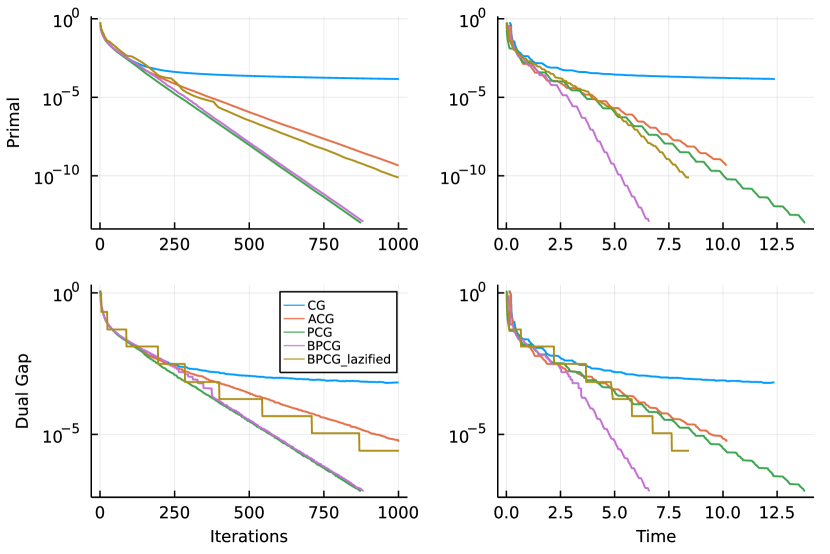
Figure 1: Probability simplex $n=200$

In addition, to assess the sparsity of generated solution of each algorithm, we also considered larger setups with $n=500$. The result are shown in Figure 2. It can be observed that both BPCG methods perform slightly (but not much) better than the others with respect to the sparsity, which is expected in this case due to known lower bounds for this type of instance (see Jaggi, [2013]).

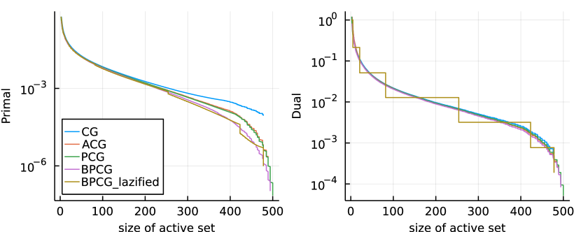
Figure 2: Sparsity: Probability simplex $n=500$

Birkhoff polytope

Let $B(n)$ be the Birkhoff polytope in $\mathbb{R}^{n\times n}$, which is the set of $n\times n$ real values matrices whose entries are all nonnegative and whose rows and columns each add up to $1$. We consider the following optimization problem

$$\min_{X\in\mathbb{R}^{n\times n}}\ \|X-X_{0}\|_{2}^{2}$$

$$\mathrm{s.t.}\ X\in B(n),$$

where $X_{0}\in\mathbb{R}^{n\times n}$. The result is Figure 3:

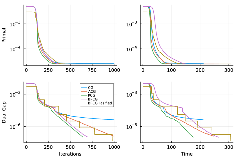
Figure 3: Birkhoff polytope $n=200$

For the primal value, the five methods have almost same performance. For the dual gap, we see that the Pairwise variant and BPCG are superior to other methods for the number of iterations and for computational time. Here the pairwise variant performed best.

In addition, we compare solution sparsity in Figure 4. The two BPCG algorithms perform much better than other methods in terms of the sparsity.

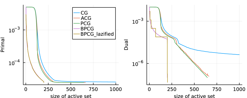
Figure 4: Sparsity: Birkhoff polytope $n=200$

Matrix completion

We also considered matrix completion instances over the spectrahedron $S=\{X\succeq 0\mid\mathrm{Tr}(X)=1\}\subset\mathbb{R}^{n\times n}$. The problem is written as

$$\min_{X\in S}\sum_{(i,j)\in L}(X_{i,j}-T_{i,j})^{2},$$

where $D=\{T_{i,j}\mid(i,j)\in L\}$ is an observed data set. We used the data set MovieLens Latest Datasets http://files.grouplens.org/datasets/movielens/ml-latest-small.zip. The result is given in Figure 5.

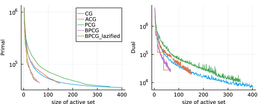
Figure 5: Sparsity: Matrix completion

We can observe the effectiveness of BPCG methods in obtaining very sparse solutions.

$\ell_{p}$ norm ball

We define the $\ell_{p}$ norm for $p\in\mathbb{R}$ and $x=(x_{1},\ldots,x_{n})\in\mathbb{R}^{n}$ as $\|x\|_{p}=\left(\sum_{i=1}^{n}|x_{i}|^{p}\right)^{\frac{1}{p}}$ and consider the following optimization problem

$$\min_{x\in\mathbb{R}^{n}}\ \|x-x_{0}\|_{2}^{2}$$

$$\mathrm{s.t.}\ \|x\|_{p}\leq 1,$$

where $\|x_{0}\|_{p}\leq 1$. We performed the numerical experiments with $p=5$ and $n=1000$. The result is given in Figure 6. The sparsest solution was obtained via BPCG methods.

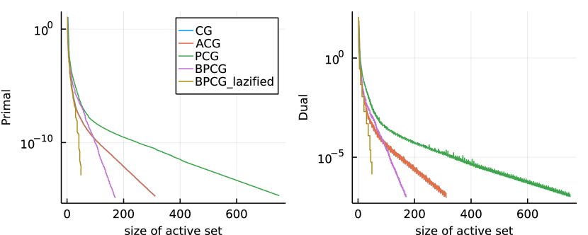
Figure 6: Sparsity: $\ell_{5}$ norm case

Note that in this experiment the vanilla Conditional Gradient and Away-step Conditional Gradient behave in exactly the same way and the blue line and orange line in the figure overlap each other.

5.2 Kernel herding

Next, we show the results of the application of BPCG to the kernel herding. We compare the BPCG algorithm and the lazified version with the ordinary kernel herding methods “linesearch” and “equal-weight” which correspond to the vanilla Frank Wolfe algorithm whose step size $\alpha_{t}$ is defined by line search and $\alpha_{t}=\frac{1}{t+1}$. In addition, we compare BPCG with the Away and Pairwise variants of “linesearch”; recall that for the latter a theoretical convergence in the infinite-dimensional case is not known. To evaluate the application of BPCG to kernel herding as a quadrature method, we compare it with the popular kernel quadrature method Sequential Bayesian Quadrature (SBQ) [Huszár and Duvenaud,, 2012] as well as the Monte Carlo method.

5.2.1 Matérn kernel case

We consider the case that the kernel is the Matérn kernel, which has the form

$$K(x,y)=\frac{2^{1-\nu}}{\Gamma(\nu)}\left(\sqrt{2\nu}\frac{\|x-y\|_{2}}{\rho}\right)^{\nu}B_{\nu}\left(\sqrt{2\nu}\frac{\|x-y\|_{2}}{\rho}\right),$$

where $B_{\nu}$ is the modified Bessel function of the second kind and $\rho$ and $\nu$ are positive parameters. The Matérn kernel is closely related to Sobolev space and the RKHS $\mathcal{H}_{K}$ generated by the kernel with smoothness $\nu$ is norm equivalent to the Sobolev space with smoothness $s=\nu+\frac{d}{2}$ (see e.g. Kanagawa et al., [2018], Wendland, [2004]). In addition, the optimal convergence rate of the MMD in Sobolev space is known as $n^{-\frac{s}{d}}$ [Novak,, 2006]. In this section, we use the parameter $(\rho,\nu)=(\sqrt{3},\frac{3}{2}),(\sqrt{5},\frac{5}{2})$ since the kernel has explicit forms with these parameters.

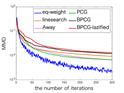
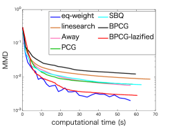
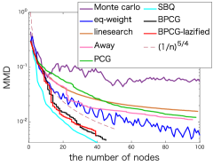
(a) MMD for the number of iterations (b) MMD for computational time

(c) MMD for the number of nodes

Figure 7: Matérn kernel ($\nu=3/2$)

The domain $\Omega$ is $[-1,1]^{d}$ and the probability distribution is a uniform distribution. First, we see the case $\nu=\frac{3}{2}$ and $d=2$. In this case, the optimal rate is $n^{-\frac{5}{4}}$. The result is Figure 7. For sparsity, BPCG methods have significant performance and they achieve the convergence speed comparable to the optimal rate. For computational time, the lazified BPCG have good performance. This is because in the lazified algorithm, we only access the active set and this reduces the computational cost considerably. Although, BPCG methods are not superior to other methods for the number of the iterations, we can see the effectiveness of BPCG methods.

Moreover, the same good performance can be seen in the case $\nu=\frac{5}{2}$ and $d=2$, which is shown in Figure 8. BPCG algorithms also achieves the convergence rate which is competitive with the optimal rate $n^{-\frac{7}{4}}$.

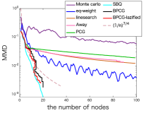
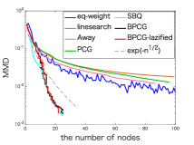
Figure 8: Matérn kernel ($\nu=5/2$) (left) and Gaussian kernel (right)

5.2.2 Gaussian kernel

Next, we treat the gaussian kernel $K(x,y)=\mathrm{exp}(-\|x-y\|_{2}^{2})$. The domain is $\Omega=[-1,1]^{d}$ and the density function of the distribution on $\Omega$ is $\frac{1}{C}\mathrm{exp}\left(-\|x\|^{2}\right)$, where $C=\int_{\Omega}\mathrm{exp}\left(-\|x\|^{2}\right)\mathrm{d}x$. In this case, we see the case $d=2$ and the result is Figure 8. We note that $\mathrm{exp}(-n^{\frac{1}{2}})$ is the exponential factor of the upper bound of convergence rate which appears in several works on gaussian kernel, for example, Wendland, [2004], Karvonen et al., [2021]. We see that BPCG methods are competitive with SBQ and the $\mathrm{exp}(-n^{\frac{1}{2}})$ rate and outperform significantly other methods.

In addition, we performed the experiments for a mixture Gaussians on $[-1,1]^{2}$. As shown in Figure 9, we have almost the same result as that of the ordinary Gaussian distribution. We note that in the left figure in Figure 9, the distribution function takes large values as the color gets closer to yellow and takes small values as the color gets closer to blue.

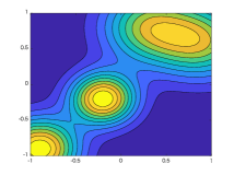
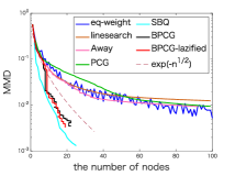
Figure 9: Contour of the mixture gausssian distribution (left) and MMD for the number of nodes(right).

6 Conclusion

The proposed Blended Pairwise Conditional Gradient (BPCG) algorithms yields very sparse solutions fast with very high speed both in convergence in iterations as well as time. It does not exhibit any swap steps, which provides state-of-the-art convergence guarantees for the strongly convex case as well as applies application to the infinite-dimensional case. We have analyzed its convergence property and exemplified its real performance via the numerical experiments. The BPCG works well for application to kernel herding, the infinite-dimensional case, in that it provides small MMD with a small number of nodes. A main avenue for future work will be tighter estimates for the convergence rate of the BPCG in various cases, in particular with regards to sparsity.

References

• Bach et al., [2012] Bach, F., Lacoste-Julien, S., and Obozinski, G. (2012). On the equivalence between herding and conditional gradient algorithms. In Proceedings of the 29th International Coference on International Conference on Machine Learning, ICML’12, pages 1355–1362, Madison, WI, USA. Omnipress.
• [2] Braun, G., Pokutta, S., Tu, D., and Wright, S. (2019a). Blended conditional gradients: the unconditioning of conditional gradients. In Proceedings of the 36th International Conference on Machine Learning (PMLR), volume 97, pages 735–743.
• Braun et al., [2017] Braun, G., Pokutta, S., and Zink, D. (2017). Lazifying conditional gradient algorithms. In Proceedings of the 34th International Conference on Machine Learning, pages 566–575.
• [4] Braun, G., Pokutta, S., and Zink, D. (2019b). Lazifying conditional gradient algorithms. Journal of Machine Learning Research (JMLR), 20(71):1–42.
• Briol et al., [2019] Briol, F.-X., Oates, C. J., Girolami, M., Osborne, M. A., and Sejdinovic, D. (2019). Rejoinder: Probabilistic Integration: A Role in Statistical Computation? Statistical Science, 34(1):38 – 42.
• Chen et al., [2010] Chen, Y., Welling, M., and Smola, A. (2010). Super-samples from kernel herding. In Proceedings of the Twenty-Sixth Conference on Uncertainty in Artificial Intelligence, UAI’10, pages 109–116, Arlington, Virginia, USA. AUAI Press.
• Combettes and Pokutta, [2020] Combettes, C. W. and Pokutta, S. (2020). Boosting Frank-Wolfe by chasing gradients. In Proceedings of the 37th International Conference on Machine Learning, pages 2111–2121.
• Frank and Wolfe, [1956] Frank, M. and Wolfe, P. (1956). An algorithm for quadratic programming. Naval Research Logistics Quarterly, 3(1–2):95–110.
• Guélat and Marcotte, [1986] Guélat, J. and Marcotte, P. (1986). Some comments on Wolfe’s ‘away step’. Mathematical Programming, 35(1):110–119.
• Huszár and Duvenaud, [2012] Huszár, F. and Duvenaud, D. (2012). Optimally-weighted herding is bayesian quadrature. In Proceedings of the Twenty-Eighth Conference on Uncertainty in Artificial Intelligence, UAI’12, pages 377–386, Arlington, Virginia, USA. AUAI Press.
• Jaggi, [2013] Jaggi, M. (2013). Revisiting Frank-Wolfe: projection-free sparse convex optimization. In Proceedings of the 30th International Conference on Machine Learning, pages 427–435.
• Kanagawa et al., [2018] Kanagawa, M., Hennig, P., Sejdinovic, D., and Sriperumbudur, B. K. (2018). Gaussian processes and kernel methods: A review on connections and equivalences. arXiv preprint arXiv:1807.02582.
• Karvonen et al., [2021] Karvonen, T., Oates, C., and Girolami, M. (2021). Integration in reproducing kernel hilbert spaces of gaussian kernels. Mathematics of Computation.
• Kerdreux et al., [2019] Kerdreux, T., d’Aspremont, A., and Pokutta, S. (2019). Restarting Frank-Wolfe. In Proceedings of the 22nd International Conference on Artificial Intelligence and Statistics, pages 1275–1283.
• Kerdreux et al., [2021] Kerdreux, T., d’Aspremont, A., and Pokutta, S. (2021). Projection-free optimization on uniformly convex sets. In Proc. Artificial Intelligence and Statistics (AISTATS).
• Lacoste-Julien and Jaggi, [2015] Lacoste-Julien, S. and Jaggi, M. (2015). On the global linear convergence of Frank-Wolfe optimization variants. In Cortes, C., Lawrence, N. D., Lee, D. D., Sugiyama, M., and Garnett, R., editors, Advances in Neural Information Processing Systems 28, pages 496–504. Curran Associates, Inc.
• Lacoste-Julien et al., [2015] Lacoste-Julien, S., Lindsten, F., and Bach, F. (2015). Sequential kernel herding: Frank-wolfe optimization for particle filtering. In Artificial Intelligence and Statistics, pages 544–552. PMLR.
• Levitin and Polyak, [1966] Levitin, E. S. and Polyak, B. T. (1966). Constrained minimization methods. USSR Computational Mathematics and Mathematical Physics, 6(5):1–50.
• Mortagy et al., [2020] Mortagy, H., Gupta, S., and Pokutta, S. (2020). Walking in the Shadow: A New Perspective on Descent Directions for Constrained Minimization. to appear in Proceedings of NeurIPS.
• Novak, [2006] Novak, E. (2006). Deterministic and stochastic error bounds in numerical analysis.
• Oettershagen, [2017] Oettershagen, J. (2017). Construction of optimal cubature algorithms with applications to econometrics and uncertainty quantification.
• Pedregosa et al., [2020] Pedregosa, F., Negiar, G., Askari, A., and Jaggi, M. (2020). Linearly convergent Frank–Wolfe with backtracking line-search. In Proc. Artificial Intelligence and Statistics (AISTATS).
• Rinaldi and Zeffiro, [2020] Rinaldi, F. and Zeffiro, D. (2020). A unifying framework for the analysis of projection-free first-order methods under a sufficient slope condition. arXiv preprint arXiv:2008.09781.
• Tsuji and Tanaka, [2021] Tsuji, K. and Tanaka, K. (2021). Acceleration of the kernel herding algorithm by improved gradient approximation. arXiv preprint arXiv:2105.07900.
• Welling, [2009] Welling, M. (2009). Herding dynamical weights to learn. In Proceedings of the 26th Annual International Conference on Machine Learning, pages 1121–1128.
• Wendland, [2004] Wendland, H. (2004). Scattered data approximation, volume 17. Cambridge university press.
• Wolfe, [1970] Wolfe, P. (1970). Convergence theory in nonlinear programming. In Integer and Nonlinear Programming, pages 1–36. North-Holland, Amsterdam.