Yongqiang Tang, Boston, USA
E-mail: yongqiang_tang@yahoo.com
MOVER confidence intervals for a difference or ratio effect parameter under stratified sampling
Abstract
[Summary] Stratification is commonly employed in clinical trials to reduce the chance covariate imbalances and increase the precision of the treatment effect estimate. We propose a general framework for constructing the confidence interval (CI) for a difference or ratio effect parameter under stratified sampling by the method of variance estimates recovery (MOVER). We consider the additive variance and additive CI approaches for the difference, in which either the CI for the weighted difference, or the CI for the weighted effect in each group, or the variance for the weighted difference is calculated as the weighted sum of the corresponding stratum-specific statistics. The CI for the ratio is derived by the Fieller and log-ratio methods. The weights can be random quantities under the assumption of a constant effect across strata, but this assumption is not needed for fixed weights. These methods can be easily applied to different endpoints in that they require only the point estimate, CI, and variance estimate for the measure of interest in each group across strata. The methods are illustrated with two real examples. In one example, we derive the MOVER CIs for the risk difference and risk ratio for binary outcomes. In the other example, we compare the restricted mean survival time and milestone survival in stratified analysis of time-to-event outcomes. Simulations show that the proposed MOVER CIs generally outperform the standard large sample CIs, and that the additive CI approach performs better than the additive variance approach. Sample SAS code is provided in the Supplementary Material.
keywords:
Additive confidence interval approach; Additive variance approach; Delta method; Fieller method; Mantel-Haensze estimator; Minimum risk weight; Non-constant effect; Restricted mean survival time1 Introduction
In clinical trials, randomization is often performed by stratifying on a few prognostic factors. For example, in the belimumab trial for systemic lupus erythematosus 1, subjects were stratified by a screening SELENA–SLEDAI score ( 9 versus 10), complement level (those with versus those without low C3 and/or C4), and race (black versus non-black). Literature reviews have been conducted to assess the usefulness of stratified randomization 2, and the reporting and analyses of stratified clinical trials 3. Stratification serves two purposes 4. First, it prevents imbalances between treatment groups in stratification factors. When there is a chance imbalance in important prognostic factors under simple randomization, the response could be different between treatment groups even if the two treatments have the same effect 5. The treatment effect estimate without adjustment for such imbalance tends to be biased. Second, stratification improves the precision of the treatment effect estimate 6, 7, 8, 9, 10. Although the post-stratification is as efficient as the pre-stratification in large samples 11, pre-stratification can be much more efficient than the post-stratification in small and moderate samples 6, 7, 8, 9, 10, and permit meaningful subgroup analyses 4 since randomization is applied to each stratum.
The method of variance estimates recovery (MOVER), originally developed by Howe 12 for constructing the confidence interval (CI) for the mean of the sum of two independent variables, becomes popular since it was generalized to the difference and ratio effect parameters 13, 14, 15. Sometimes, the Wald approach might be the only simple direct interval estimation method in complex situations such as the comparison of the restricted mean survival time (RMST) on the basis of the nonparametric Kaplan-Meier (KM) technique. However, it is straightforward to use the MOVER technique, in which the CI for RMST is derived for each group, and combined into the CI for the difference or ratio of RMST between two groups 16. One selects a single sample CI (e.g. score type CIs) with good properties, which will be inherited by the MOVER CI for the comparison of two groups. The MOVER method generally performs well compared to other asymptotic approaches in finite samples 13, 17, 14, 16.
The purpose of the paper is to propose a general framework for constructing MOVER CIs for a difference and ratio effect parameter under stratified sampling. We derive the additive variance (AV) and additive CI (AC) approaches for the difference parameter. They require only the point estimate, CI, and variance estimate for the parameter of interest in each group across strata. The AV approach relies on the delta method, in which the variance for the weighted difference is calculated as the sum of the MOVER variance for the difference in each stratum. Although the variability in the weight is ignored, the AV approach is asymptotically valid for random weights such as the inverse variance (INV) weight when the effect is constant across strata.
In the AC approach, the CI of the weighted sum statistic is calculated as the sum of the stratum-specific -level CI for an appropriate by ignoring the variability in the weights. There are two variations (labeled as “AC” and “AC2”). In AC, the CI is constructed for the summary effect in each group, and then combined into the MOVER CI for the difference between two groups. In AC2, we derive the MOVER or other CIs for the stratum-specific difference, and combine them into the CI for the weighted difference.
The CI for the ratio is obtained by the Fieller or log-ratio method. A concern with the Fieller CI is that it may be disjoint, and hence difficult to interpret 18. We show the Fieller CI is non-disjoint and uniquely determined if the parameter of interest takes only positive values, and this applies to binary proportions, Poisson rates or mean survival. The proposed MOVER CIs are asymptotically valid for random weights if the difference or ratio is constant across strata, or for non-constant effects when the weights are fixed.
The rest of the paper is organized as follows. We introduce the general MOVER methods under stratified sampling in Section 2. Real data analyses and simulations are given respectively in sections 3 and 4.
2 MOVER intervals under stratified sampling
2.1 Review of MOVER CIs in unstratified samples
We are interested in the risk difference (RD) between two independent groups (). The CI for is . The MOVER Cl for is constructed as
| (1) |
where the symbol with denotes the point estimate. Let be the variance of . The underlying idea 14 is that the variance can be recovered as or , where is the -th percentile of the normal distribution. One shall choose a one-sample CI with good properties. Examples include the score type CI for binary 13, Poisson 19 and survival 16 outcomes, and the exact CI for variance components related to the multivariate normal distribution 17. The MOVER CI in Equation (1) is asymptotically equivalent to the Wald CI, but the MOVER CI generally has a better performance in finite samples.
2.2 Weighted difference
As shown in Appendix A, the unstratified RD estimate is generally biased under stratified sampling. We describe a general framework for constructing the CI for a difference or ratio effect parameter in stratified studies. Subjects in different strata and groups are assumed to be independent. Let denote the set of model parameters for stratum , and . Suppose we want to construct the CI for the weighted difference
| (2) |
where is a function of , and . We set if the difference is of interest. In general, denotes the ratio . In the Fieller CI approach for the ratio, the CI for is needed given , and the details will be given in Section 2.3. We assume although the constraint is not necessary in calculating the ratio .
Let be the sample size in group stratum , the variance for , the CI for , and the estimated weight. The total sample size is .
We illustrate the problem by a bioassay study 20 in evaluating the carcinogenic effect on four sex-strain groups of mice. The number of responders and mice in the four strata are presented below
| stratum | 1 | 2 | 3 | 4 |
|---|---|---|---|---|
| control | 5/79 | 3/87 | 10/90 | 3/82 |
| treated | 4/16 | 2/16 | 4/18 | 1/15 |
Let be the proportion in group strata . Then and . The weighted RD estimator is given by
| (3) |
with the MH, INV and MR weights. The MH weight is fixed while the INV and MR weights are random quantities depending on ’s. The MOVER CIs are constructed on the basis of the single sample estimates , and the Wilson score interval13 for .
The AV, AC and AC2 CIs for rely on two lemmas and one corollary established in the remaining of this section. Their proofs are given in the appendix. The weight shall not depend on after normalization by the total weight. Otherwise, the Taylor series approximation underlying the delta method for Lemma 2.1 may fail. For this reason, Lemma 2.1 is not suitable for the MR weight, and this will be illustrated in Section 4.
Lemma 2.1.
Assume both functions and are continuous and differentiable at .
Suppose has a limiting normal distribution.
a.) The asymptotic variance of is given by
It is also the variance for when ’s are fixed, or when .
b.)
If ’s are fixed, or if in all strata for a known ,
the asymptotic variance of is
c.) Under the assumption in (b), the asymptotic variance of is given by
While Lemma 2.1b seems obvious when ’s are fixed, its merit lies in its validity for a common difference or ratio parameter across strata when the weights are random quantities. Lemma 2.1c gives the variance for the log ratio of two weighted means.
In the AV approach, the variance of is recovered in an additive form as or according to Lemma 2.1b. The AV CI for is
Lemma 2.2.
Suppose the level CI for is , where is the variance of ,
is a consistent variance estimate, and
.
Let .
If is consistently estimated by and , then
a) and
b) Both and are consistent estimators of .
By Lemma 2.2a and Lemma 2.1b, the MOVER CI for is given by
| (4) |
This CI is referred to as the AC CI since is the CI for , and the weighted sum of the stratum-specific CIs for when the weights are fixed or there is no stratum effect (). However, when there is a stratum effect, the CI in Equation (4) is still valid for random weights if the difference is constant.
Lemma 2.2a is a generalization of Yan and Su (YS 21) result for binomial proportions. There are several issues in the YS method 21. First, is treated as the CI for , and this is incorrect for random weights ’s when there is stratum effect. The YS MOVER CI takes the form
where , , and . The YS CI tends to overcover (conservative) if the response rates vary greatly across strata, and this will be shown in Section 4. YS 21 suggested optimal weights for each group. When the weights differ between two groups, the CI defined in Equation (4) may be invalid for a constant difference when there is a stratum effect.
Corollary 2.3.
Let be a consistent variance estimate for , and the level CI for , where . Then is the CI of if the weights ’s are fixed, or if the difference is constant across strata.
The AC2 CI is obtained from Corollary 2.3. It combines the MOVER or other CIs for the difference in each stratum into a single CI for . In the application of Lemma 2.2 and Corollary 2.3, we employ the delta variance for and . Alternatively, one may use the variance [e.g. , , ] recovered from the CI.
2.3 MOVER CIs for ratio under stratified sampling
The CI for the ratio is obtained via the Fieller or log-ratio method. In the log-ratio method, we first derive the CI for and then exponentiate it. The Fieller approach inverts the test . The Fieller CI contains all values of for which the null hypothesis is not rejected, or equivalently the CI for includes .
2.3.1 AC approach
The Fieller CI contains all values of for which the CI for given in Equation (4) includes 0. If the parameters ’s take only positive values, the Fieller CI is uniquely determined and non-disjoint. It is a consequence of the following lemma
Lemma 2.4.
The function (, , and ) decreases from to as increases from to because . There is at most one solution for , where or .
In MOVER, setting the lower and upper limits for to 0 yields the CI for the ratio,
| (5) |
where , , , , and . If , then . We have and . The solution (5) always exists since and no matter whether and .
In the log-ratio method, the MOVER CI for is obtained based on Lemma 2.2b and Lemma 2.1c, and then exponentiated
| (6) |
where , and . The log-ratio CI is incomputable if and . Otherwise it is usually similar to the Fieller CI.
We refer the Fieller and log-ratio CIs to respectively as “AC” and “ACL”. It is valid for random ’s with a constant ratio. Interestingly, the ratio does not have to be the same across strata for fixed (e.g. MH) weights.
2.3.2 AC2 approach
Setting the limits of the AC2 CI for to 0 yields the Fieller CI for . The lower limit is if . The upper limit is if . In general, there is no explicit analytic solution for the confidence limits. They may be solved by the bisection method by using the AC confidence limit as the initial value.
2.3.3 AV approach
In the log-ratio method, the variance of is given by Lemma 2.1c, and the CI is
| (8) |
where is the asymptotic or MOVER variance for . In the MOVER approach, we replace by or .
We denote the Fieller and log-ratio CIs by “AV” and “AVL” respectively.
3 Data examples
| Risk Difference | Relative risk | ||||
| MH§ | INV | MR | MH§ | ||
| Est. | |||||
| Asymptotic CIs | |||||
| DC† | DC† | ||||
| Wald | ASY | ||||
| MOVER CIs | |||||
| AV | AV | ||||
| YS | AVL | ||||
| AC | AC | ||||
| AC2 | AC2 | ||||
| ACL | |||||
§ MH estimate of RD and RR
† Based on dually consistent variance estimate under both large strata and sparse data
Example 3.1.
We revisit the bioassay data displayed in Section 2.2. Appendix A shows that the estimated difference is generally biased in the unstratified analysis. Stratified analysis can prevent bias, and improve the precision of the treatment effect estimate 6, 7, 8, 9, 10, and are hence recommended. The MOVER CIs are compared with the asymptotic CIs on the basis of the variance valid only under large strata (labeled as “ASY” or “Wald”, formulae given in the appendix) and the dually consistent variance estimates (labeled as “DC”) valid for both sparse data and large strata 22, 23, 24. The asymptotic CIs for RR are obtained by exponentiating the CIs on the log scale. Sample SAS code is provided in the Supplementary Material.
The results are displayed in Table 1, and all methods adjust for the stratification factor. The following CIs require the constant effect assumption: 1) All DC CIs for the MH estimators; 2) All CIs for the INV weighted RD. These assumptions can not hold simultaneously. For illustration purposes, we assume the relevant assumptions hold for each method. Throughout this paper, all CIs for the MR weighted RD are corrected as to penalize for ignoring variabilities in the weight 25 even if the RD is constant, where . No continuity correction is applied to other CIs.
On both RD and RR effect metrics, the AC and AC2 approaches yield very similar CIs, and the AV CI has a larger lower confidence limit than other CIs. On the RR metric, the AVL CIs are wider than other MOVER CIs.
The Wald CI for the INV-weighted RD contains 0. All other CIs indicate there is a significant difference between two treatment groups as the lower limits for RD are above 0, and the lower limits for RR are above 1.
| One-sample CI | Difference | Ratio | |||||
| obs: control | IFN: treated | AV | AC† | AV | AVL | AC† | ACL |
| 8-year KM survival probability: | |||||||
| 8-year RMST: | |||||||
[1] For each effect measure, the first (second) row displays the one-sample CI for male (female) and the CIs for the difference and ratio on basis of the MH (INV) weight.
† The AC2 CI is very similar to the AC CI for both difference and ratio, and not displayed due to limited space
Example 3.2.
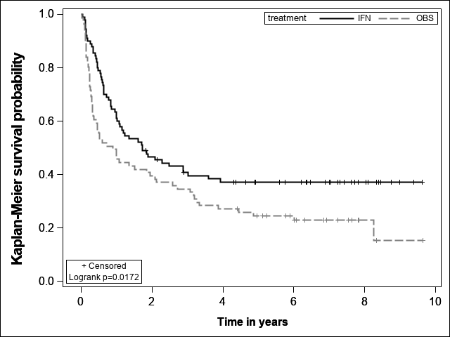
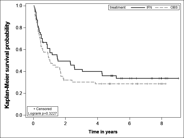
We apply the proposed method to the RMST and milestone survival for time to event outcomes. We analyze the Eastern Cooperative Oncology Group (ECOG) 1684 trial 26. Patients with American Joint Committee on Cancer stage IIB or III melanoma were randomized to receive Interferon alfa-2b (IFN) or to receive close observation (Obs). A total of 287 patients were accrued between 1984 and 1990. and remained blinded under analysis until 1993. Patients in the IFN arm had significantly improved relapse-free survival (RFS) compared with Obs.
The purpose of the analysis is to compare the 8-year KM survival and RMST for RFS between two groups stratified by sex. Figure 1 plots the KM curves for RFS by sex. Slightly earlier and larger separation in the KM curves was observed in male patients than in female subjects. We first illustrate how to assess the treatment by stratum interaction by the MOVER technique. The one-sample CI for both KM survival and RMST is obtained by inverting the so-called score-type or constrained variance test in the sense that the variance of is obtained under the null hypothesis 27, 28, 16. Table 2 presents the single-sample score type CIs for the KM survival 28 and RMST 16 by sex. The point estimate ( MOVER CI based on the score limit) for the difference of RMST is () for male, and () for female. Another application of the MOVER technique yields the CI for , which contains 0. Although a larger separation in the KM curves is observed among males than among females, the difference does not significantly differ between male and female. In general, a test of the treatment by stratum interaction requires a much larger sample size. A similar technique may be employed on the log scale to assess whether the ratio effect measure differs between male and female.
Table 2 displays the stratified MOVER CIs for the difference and ratio of the milestone survival and RMST. The MH weight is . The INV weight is for the milestone survival, and for RMST. The INV and MH weights are close to each other, and yield very similar CIs. For RMST, the lower limit is above 0 for the difference, and above 1 for the ratio, evidencing the superiority of IFN over control in prolonging the mean survival. The difference for the milestone survival is marginally significant in the sense that the lower limit is near 0 for the difference, and near 1 for the ratio.
4 Simulation
We conduct simulation to assess the proposed MOVER CIs for RD and RR in stratified analyses of binary proportions, and compare them with the asymptotic CIs. In all cases, one million datasets are simulated. A dataset will be regenerated until the following conditions hold: 1) there is at least one event in the study () on the RD metric, 2) there is at least one event in each treatment group (, ) on the RR metric. Otherwise the DC CIs for the MH estimators 10 and some MOVER CIs may be incomputable.
There is more than chance that the empirical coverage probability (CP) lies within of the true value when the target level is . This greatly reduces the random error in the estimate, and enables the detection of subtle differences between methods. When the sample size is not large, it is usually difficult to control the CP exactly at the target level. Following Tang 10, we deem the CPs to be highly satisfactory if it lies within at the nominal level.
On the RD scale, we use the estimate if , and if to calculate the INV and MR weights 22, but the difference is still computed as .
A CI is said to be asymptotically valid if the CP converges to as . Simulation may show that a method is not asymptotically valid. In Example 4.3 below, the CPs are not close to in the DC method for RD and RR under heterogeneity effect, and in the YS method for RD even when . In Example 4.4 below, the type I errors are not close to in the MR-weighted tests for RD at . These methods may not be asymptotically accurate. All other MOVER methods are asymptotically valid according to the theory in Section 2.2.
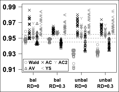
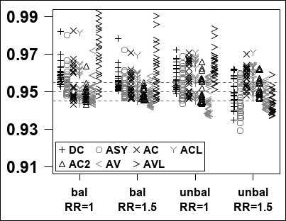
Example 4.1.
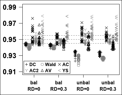
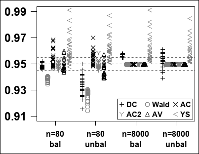
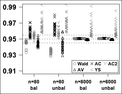
We conduct a simulation study to assess CIs for stratified comparisons of binary outcomes for a constant effect on the RD and RR scales. Suppose there are two strata. The sample sizes are either balanced or unbalanced in the two groups. The trial size is . The true response rates in the control arm are set to for . There are a total of combinations of . The true effect is 0 or 0.3 on the RD scale, and 1 or 1.5 on the RR metric. The results are displayed in Figures 2a, 2c and 2e.
RD metric: The result for the INV weight is not reported due to limited space. The DC and Wald CIs tend to undercover, and the coverage becomes much worse under unbalanced sample sizes. While both AC and AC2 maintain CP above in most cases, the AC generally yields slightly larger CP than the AC2. Although the AV method performs better than the DC and Wald methods, it yields lower than nominal CPs in quite many cases when the sample sizes are unequal.
RR metric: For the MH estimator, the DC and ASY methods yield CPs below the nominal level in about half of cases at under unbalanced sample sizes, and work well in other situations. The AC and ACL methods produce similar results that are above in nearly all cases. The AC2 CI is slightly less conservative than the AC CI. The AV method gives CPs that are slightly below in a few cases with unbalanced sample sizes. The AVL method yields CPs above more often than other three MOVER CIs.
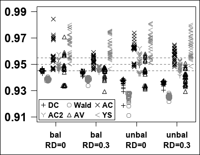
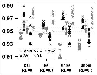
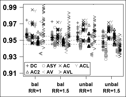
Example 4.2.
We conduct a simulation study to assess CIs for stratified comparisons of binary outcomes for a constant effect on the RD and RR scales when there are three strata. The sample sizes are either balanced or unbalanced in the two groups. The trial size is . The true response rates in the control arm are set to for . There are a total of combinations of . The results are displayed in Figures 2b, 2d and 2f, and the result pattern is fairly similar to that observed in Example 4.1.
Example 4.3.
Simulation is conducted to demonstrate that the MOVER CIs for the MH estimator of RD and RR do not require the assumption of a constant effect. For RR, the MH estimate is the ratio of the MH weighted proportions between two groups. When the group size ratio is constant across strata (commonly used in large clinical trials), the MH estimate is identical to the crude RR estimate from the unstratified analysis, but a stratified analysis improves the precision of the RR estimate 22.
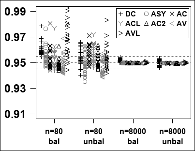
We use a similar simulation setup to example 4.1 except for the following differences. The true RD is , or the true RR is in the two strata. The total size is either or , but the group size ratio remains the same. We assess whether each CI contains the pooled difference on the RD metric, or the ratio of the pooled proportion on the RR metric, where . Figures 3 shows the results. The result for the MR weight on the RD metric is also reported since the MR weighting scheme is specially designed to handle non-constant RDs 25.
At , all CIs except the YS method for RD and the DC methods for both RD 24 and RR 22 maintain CP in a very narrow range around , indicating the asymptotic validity of these methods in the presence of a non-constant RD or RR. The YS method is generally conservative. The DC methods require the constant effect assumption. When the RDs differ between the two strata, the MR weight defined in Equation (9) in Example 4.4 below approximates when the sample size is extremely large (constant allocation ratio across strata), and the CPs are hence well maintained around the target level.
At n=80, the ASY or Wald methods tend to undercover. The AC and AC2 methods show better performance than other approaches on the RD scale, and the AC, AC2 and AVL outperform other methods under unequal randomization on the RR metric. The AC2 CI appears to be slightly less conservative than the AC CI on both metrics.
Example 4.4.
We compare the type I error and power for testing the hypothesis on the basis of the Wald and MOVER CIs, and illustrate that the MOVER method may not be suitable for the MR weight in estimating the RD. The true proportion is , and RD=0 or 0.05 is constant across strata.
The result is presented in Table 3. The YS 21 approach yields the two-sided type I error far below the target level under , and produces lower power than other approaches at in all cases. For both MH and INV weights, the AC, AC2 and AV approaches have nearly nominal type I error rates, evidencing the asymptotic validity of these MOVER approaches for both fixed and random weights.
The MR weight slightly inflates the type I error rates at and . In this scenario, the empirical mean weight standard deviation in stratum is for the MR weight, and for the INV weight based on simulated datasets. For a constant RD, the MR weight 25
| (9) |
does not actually converge to the limit of the INV weight since does not converge in probability to 0, where , and . The MR weight is not as powerful as the INV weight in detecting a constant RD.
Lemma 2.1 is suitable for the INV weight, but not for the MR weight. The MR weight depends on both and , but the INV weight depends only on ’s. At , the type I error rate is inflated in the MR-weighted approaches because the variability in the MR weight is ignored, and the continuity correction of Mehrotra and Railkar 25 has a negligible effect on the inference in extremely large samples.
[1] The sample sizes are the same in each group across strata
[2] The correction method of Mehrotra and Railkar (2000) is applied to all CIs for the MR weight
| MH weight | INV weight | MR weight | |||||||||||||
|---|---|---|---|---|---|---|---|---|---|---|---|---|---|---|---|
| Wald | YS | AV | AC | AC2 | Wald | YS | AV | AC | AC2 | Wald | YS | AV | AC | AC2 | |
| two-sided type I error (): true RD=0 | |||||||||||||||
| 50 | 5.43 | 2.01 | 4.79 | 4.64 | 4.88 | 5.53 | 1.19 | 4.44 | 4.96 | 5.08 | 5.36 | 1.42 | 5.21 | 4.61 | 4.83 |
| 100 | 5.24 | 2.21 | 4.91 | 4.88 | 4.97 | 5.25 | 1.20 | 4.78 | 5.16 | 5.10 | 5.39 | 1.49 | 5.50 | 5.12 | 5.13 |
| 200 | 5.13 | 2.13 | 4.98 | 4.97 | 5.00 | 5.15 | 1.18 | 4.89 | 5.09 | 5.05 | 5.44 | 1.60 | 5.62 | 5.31 | 5.32 |
| 500 | 5.10 | 2.19 | 5.04 | 5.04 | 5.05 | 5.20 | 1.21 | 5.10 | 5.17 | 5.16 | 5.56 | 1.63 | 5.74 | 5.52 | 5.52 |
| 10000 | 5.03 | 2.15 | 5.03 | 5.03 | 5.03 | 5.05 | 1.18 | 5.05 | 5.05 | 5.05 | 5.67 | 1.71 | 5.74 | 5.67 | 5.67 |
| power (): true RD=0.05 | |||||||||||||||
| 50 | 14.2 | 7.5 | 13.4 | 13.1 | 13.6 | 15.8 | 6.5 | 14.4 | 15.1 | 15.2 | 14.4 | 6.4 | 14.7 | 13.4 | 13.7 |
| 100 | 23.0 | 13.9 | 22.5 | 22.3 | 22.6 | 25.9 | 12.7 | 25.0 | 25.5 | 25.5 | 24.3 | 12.6 | 24.9 | 23.8 | 23.9 |
| 200 | 40.2 | 28.3 | 40.0 | 39.8 | 40.0 | 45.4 | 27.3 | 44.8 | 45.2 | 45.1 | 43.2 | 27.1 | 44.0 | 42.9 | 43.0 |
| 500 | 77.1 | 65.8 | 77.0 | 77.0 | 77.0 | 82.7 | 67.8 | 82.6 | 82.7 | 82.7 | 80.7 | 66.7 | 81.1 | 80.6 | 80.6 |
5 Discussion
We propose several MOVER CIs for a difference or ratio parameter under stratified sampling. These approaches require only the single sample point estimate, variance estimate and CI for the parameter of interest in each stratum, and hence can be easily applied to different outcomes. For the difference parameter, either the CI for the weighted difference, or the CI for the weighted effect in each group, or the variance for the weighted difference is calculated as the sum of the corresponding stratum-specific statistics. The CIs for the ratio are derived by the Fieller or log-ratio approaches. The Fieller CI for the ratio of proportion, rate or mean survival can be uniquely determined and non-disjoint. All these interval estimation methods except the AC2 CI for a ratio are non-iterative.
We apply the MOVER CIs to the binary and survival outcomes. As demonstrated by several simulation studies, the proposed MOVER approaches generally outperform the asymptotic CIs. The YS21 MOVER CI for RD is conservative particularly when the proportions vary greatly across strata. In general, the AC and AC2 approaches show better performance than the AV approach for both difference and ratio parameters. For binary outcomes, the AC2 CI tends to be slightly less conservative for the MH estimators of RD and RR than the AC CI. For the ratio, the Fieller CI is preferable over the log-ratio CI. The log-ratio CI is incomputable if the point estimate or is 0. Otherwise, the ACL and AC CIs are generally similar. The AVL approach appears to be more conservative than the AV method. In summary, we recommend the AC and AC2 interval estimation methods for the difference, and the Fieller approach for the ratio.
The proposed MOVER CIs are asymptotically valid for random weights under the assumption of a constant difference or ratio across strata, or for non-constant effects when the weights are fixed. However, this does not work for the MR-weighted RD for binary outcomes, and the reasons are given in Example 4.4. The continuity correction suggested by Mehrotra and Railkar 25 for penalizing for ignoring variability in the MR weight improves the performance in small and moderate samples, but the CP of the CI may slightly deviate from the nominal level when the RD is constant in extremely large samples.
Appendix A Ignoring stratification may lead to biased estimate
We assess the bias of the unstratified RD estimate in data with two strata. The true proportion is in group stratum . The true RD between two groups is in both strata. That is, .
Let be the number of subjects in group stratum . Let . In the unstratified analysis, the expectation of the estimated RD is
The expected difference in the unstratified analysis is only if (i.e. no stratification effect) or (the sample size ratio between two groups is constant in the two strata). If the risk in the control arm differs between two strata (i.e. ), but there is imbalance in the stratification factor between two groups (equivalently ), the unstratified analysis is biased.
Appendix B Proof of two lemmas
Proof B.1 (Proof of Lemma 2.1).
Proof B.2 (Proof of Lemma 2.2).
It is easy to see the following asymptotic relationships
The last equation is obtained by Taylor series expansion of around . The remaining relationships can be proved similarly.
Appendix C Large sample variance for MH estimates
References
- 1 Stohl W, Schwarting A, Okada M, et al. Efficacy and Safety of Subcutaneous Belimumab in Systemic Lupus Erythematosus: A Fifty-Two–Week Randomized, Double-Blind, Placebo-Controlled Study. Arthritis Rheumatol 2017; 69: 1016 - 27.
- 2 Kernan WN, Viscoli CM, Makuch RW, Brass LM, Horwitz RI. Stratified randomization for clinical trials. Journal of Clinical Epidemiology 1999; 52: 19-26.
- 3 Kahan BC, Morris TP. Reporting and analysis of trials using stratified randomisation in leading medical journals: review and reanalysis. British Medical Journal 2012; 345: e5840.
- 4 EMA . Guideline on adjustment for baseline covariates in clinical trials. Available at https://www.ema.europa.eu/en/documents/scientific-guideline/guideline-adjustment-baseline-covariates-clinical-trials_en.pdf . 2015.
- 5 Chu R, Walter SD, Guyatt G, et al. Assessment and Implication of Prognostic Imbalance in Randomized Controlled Trials with a Binary Outcome - A Simulation Study. Plus One 2012; 7: e36677.
- 6 Grizzle JE. A note on stratifying versus complete random assignment in clinical trials. Controlled Clinical Trials 1982; 3: 365-8.
- 7 McHugh R, Matts J. Post-Stratification in the Randomized Clinical Trial. Biometrics 1983; 39: 217 - 25.
- 8 Miratrix LW, Sekhon JS, Yu B. Adjusting Treatment Effect Estimates by Poststratification in Randomized Experiments. Journal of the Royal Statistical Society, Series B 2013; 75: 369-96.
- 9 Tang Y. Exact and Approximate Power and Sample Size Calculations for Analysis of Covariance in Randomized Clinical Trials With or Without Stratification. Statistics in Biopharmaceutical Research 2018; 10: 274 - 86.
- 10 Tang Y. Score confidence intervals and sample sizes for stratified comparisons of binomial proportions. Statistics in Medicine 2020; 39: 3427 - 57.
- 11 Peto R, Pike MC, Armitage P, et al. Design and analysis of randomized clinical trials requiring prolonged observation of each patient. II. analysis and examples. British Journal of Cancer 1977; 35: 1 - 39.
- 12 Howe WG. Approximate confidence limits on the mean of X+Y where X and Y are two tabled independent random variables. Journal of the American Statistical Association 1974; 69: 789 - 94.
- 13 Newcombe RG. Interval estimation for the difference between independent proportions: comparison of eleven methods. Statistics in Medicine 1998; 17: 873 - 90.
- 14 Donner A, Zou GY. Closed-form confidence intervals for functions of the normal mean and standard deviation. Statistical Methods in Medical Research 2012; 21: 347 - 59.
- 15 Newcombe RG. MOVER-R confidence intervals for ratios and products of two independently estimated quantities. Statistical Methods in Medical Research 2016; 25: 1774 -8.
- 16 Tang Y. Some new confidence intervals for Kaplan-Meier based estimators from one and two sample survival data. Statistics in Medicine 2021.
- 17 Lee Y, Shao J, Chow SC. Modified Large-Sample Confidence Intervals for Linear Combinations of Variance Components. Journal of the American Statistical Association 2004; 99: 467 - 78.
- 18 Sherman M, Maity A, Wang S. Inferences for the ratio: Fieller’s interval, log ratio, and large sample based confidence intervals. AStA Advances in Statistical Analysis 2011; 95: article 313.
- 19 Li HQ, Tang ML, Wong WK. Confidence intervals for ratio of two Poisson rates using the method of variance estimates recovery. Computational Statistics 2014; 29: 869-89.
- 20 Gart JJ. Analysis of the common odds ratio: corrections for bias and skewness. In: . 45th of Book 1. Springer; 1985: 175 - 76.
- 21 Yan X, Su G. Stratified Wilson and Newcombe confidence intervals for multiple binomial proportions. Statistics in Biopharmaceutical Research 2010; 2: 329 - 35.
- 22 Greenland S, Robins JM. Estimation of a Common Effect Parameter from Sparse Follow-Up Data. Biometrics 1985; 41: 55 - 68.
- 23 Robins JM, Breslow N, Greenland S. Estimators of the Mantel-Haenszel variance consistent in both sparse data and large strata limiting models. Biometrics 1986; 42: 311 - 23.
- 24 Sato T. On the variance estimator for the Mantel-Haenszel risk difference (letter). Biometrics 1989; 45: 1323 - 24.
- 25 Mehrotra D, Railkar VR. Minimum risk weights for comparing treatments in stratified binomial trials. Statistics in Medicine 2000; 32: 811 - 25.
- 26 Kirkwood JM, Strawderman MH, Ernstoff MS, Smith TJ, et al . Interferon alfa-2b adjuvant therapy of high-risk resected cutaneous melanoma: the Eastern Cooperative Oncology Group trial EST1684. Journal of Clinical Oncology 1996; 14: 7-17.
- 27 Thomas DR, Grunkemeier GL. Confidence interval estimation of survival probabilities for censored data. Journal of the American Statistical Association 1975; 70: 865-871.
- 28 Barber S, Jennison C. Symmetric Tests and Confidence Intervals for Survival Probabilities and Quantiles of Censored Survival Data. Biometrics 1999; 55: 430-436.